On the maximum mass of magnetised white dwarfs

Abstract

We develop a detailed and self-consistent numerical model for extremely-magnetised white dwarfs, which have been proposed as progenitors of overluminous Type Ia supernovae. This model can describe fully-consistent equilibria of magnetic stars in axial symmetry, with rotation, general-relativistic effects and realistic equations of state (including electron-ion interactions and taking into account Landau quantisation of electrons due to the magnetic field). We study the influence of each of these ingredients onto the white dwarf structure and, in particular, on their maximum mass. We perform an extensive stability analysis of such objects, with their highest surface magnetic fields reaching $\sim 10^{13}$ G (at which point the star adopts a torus-like shape). We confirm previous speculations that although very massive strongly magnetised white dwarfs could potentially exist, the onset of electron captures and pycnonuclear reactions may severely limit their stability. Finally, the emission of gravitational waves by these objects is addressed, showing no possibility of detection by the currently planned space-based detector eLISA.

1 Introduction

White dwarfs (WDs) are the stellar remnants of low and intermediate mass stars, i.e. stars with masses $\lesssim$ 10 M_⊙ (M_⊙ being the mass of our Sun) (Shapiro & Teukolsky, 1983). The interest in WD properties and in particular their mass-radius relation has been renewed by the recent discovery of overluminous type Ia supernova (SNIa) (Howell et al., 2006; Scalzo et al., 2010; Maoz et al., 2014). The progenitors of such events are thought to be “super-Chandrasekhar” WDs with a mass $>$ 2 M_⊙ (see, e.g., Hillebrandt et al., 2013). These SNIa may result from the merger of two massive WDs or from the explosion of rapidly differentially rotating WDs (see, e.g., Howell et al., 2006). Alternatively, it has been argued that WDs endowed with a strong magnetic field could be potential candidates for the progenitors of these peculiar SNIa (Kundu & Mukhopadhyay, 2012; Das & Mukhopadhyay, 2012a, b, 2013a, 2013b; Das et al., 2013). As a matter of fact, very massive strongly magnetised WDs were proposed much earlier by Shul’man (1976); this work, however, does not seem to have attracted much attention. The existence of magnetised supermassive WD is of interest not only for astrophysics, but also for cosmology since SNIa have been used as ”standard candles” to measure cosmological distances assuming a unique astrophysical scenario for these events.

The mass-radius relation for non-magnetic WDs was established way back in 1935 by the pioneering work of Chandrasekhar, assuming a simple degenerate electron Fermi gas equation of state (EoS) at zero temperature. Subsequently, other works attempted to construct more realistic models of WDs. Apart from the magnetic field, different effects could alter the Chandrasekhar limit for the maximum mass of a WD:

• Inclusion of finite temperature (Marshak, 1940) and slow rotation (Ostriker & Hartwick, 1968) did not result in significant deviations from the Chandrasekhar WD mass-radius relation.

• The electrostatic interaction between electrons and ions introduced by Hamada & Salpeter (1961) was found to lower the electron pressure resulting in a softer EoS and hence leads to slightly less massive configurations.

• The effect of general relativity on the structure of non-magnetic WDs was found to be non-negligible, reducing by a few per cent the WD maximum mass (see, e.g., Shapiro & Teukolsky, 1983; Ibáñez, 1983, 1984; Rotondo et al., 2011; De-Hua et al, 2014; Boshkayev et al., 2015; Bera & Bhattacharya, 2016).

The existence of magnetised WDs, with magnetic fields $B\gtrsim 10^{6}$ G (Shapiro & Teukolsky, 1983), first predicted in the 1940s by Blackett (1947), was confirmed in 1970 by Kemp (see, e.g., Jordan, 2009, for a review). At the time of this writing, hundreds of magnetised WDs have already been discovered (Kepler et al., 2013). While surface magnetic fields up to about $10^{9}$ G can been inferred from Zeeman spectroscopy and polarimetry, or cyclotron spectroscopy (see, e.g., Wickramasinghe & Ferrario, 2000, for a review), internal magnetic fields are not directly accessible by observations. Therefore, very strong magnetic fields in the core of WDs, as high as $B\sim 10^{13}$ G (Fujisawa et al., 2012), cannot be ruled out from a simple estimate of the energetics (i.e. scalar virial theorem) or the conservation of magnetic flux of the progenitor star. The question therefore arises of how such a strong magnetic field affects the structure of WDs.

The study of the mass-radius relation of a magnetised WD has a long history and it was recognised early on that the impact of the magnetic field on both the stellar radius and mass could be large. However, simplifying assumptions have been made for convenience. For instance, the pioneering work by Ostriker & Hartwick (1968) considered a vanishing magnetic field at the surface of the star and neglected any magnetic field effect on the EoS as well as general relativistic effects and electrostatic interactions. The works of Adam (1986), Das & Mukhopadhyay (2012a), and Kundu & Mukhopadhyay (2012) focused on the effect of the magnetic field on the EoS, taking into account the Landau quantisation of the electron gas, but were based on a Newtonian description of the star’s structure in spherical symmetry, i.e. neglecting the deformation of the star by the magnetic field. A similar approach was followed by Suh & Mathews (2000), where, however, the (spherical) stellar structure was calculated from the general relativistic Tolman-Oppenheimer-Volkoff equations. The deformations of the star under the influence of a strong magnetic field have been recently studied by Bera & Bhattacharya (2014) in the Newtonian framework. Das & Mukhopadhyay (2015a) and Bera & Bhattacharya (2016) have computed the mass-radius relation of magnetic WDs for different magnetic field geometries within a general relativistic framework using the publicly available XNS code. On the other hand, Landau quantisation effects were neglected.

According to all these previous studies, the maximum possible mass of strongly magnetised WDs lies substantially above the Chandrasekhar limit, and more importantly above the mass inferred from observations of overluminous SNIa, see also Cheoun et al. (2013); Herrera & Barreto (2013); Herrera et al. (2014); Federbush et al. (2015); Belyaev et al. (2015). Leaving aside the origin of such strong magnetic fields – more than three orders of magnitude higher than currently observed fields –, the question as to whether such stars can possibly exist still needs to be further examined. Coelho et al. (2014); Chamel et al. (2013, 2014); Chamel & Fantina (2015) discussed various microscopic and macroscopic instabilities. In particular, Chamel et al. (2013, 2014) pointed out that the stability of very massive magnetised WDs will not only be limited by general relativity, but also by electron captures by nuclei and pycnonuclear reactions in the stellar core. These microscopic processes, whose onset depends on the magnetic field strength (Chamel & Fantina, 2015), should thus be carefully considered in modelling massive magnetised WDs.

In this study, we address these stability issues. To this end, we shall construct consistent global general relativistic models of strongly magnetised WDs, taking into account the magnetic field effects on both the EoS and the WD equilibrium structure equations. This work follows directly from our previous study of the structure of strongly magnetised neutron stars (Chatterjee et al., 2015). We shall account for the onset of electron capture and pycnonuclear reactions, including the shifts on the threshold densities and pressures due to electron-ion interactions and to the strong magnetic field. Recently, during the refereeing process of our paper, a very similar independent study by Otoniel et al. (2016) appeared in the literature.

The paper is organised as follows. In Sec. 2 we describe the realistic dense matter EoS we considered, taking into account both the effects of electron-ion interactions and the presence of the magnetic field. In Sec. 3, we summarise the modified Maxwell equations and the hydrodynamic equations in presence of a magnetic field in general relativity and Newtonian theory. In Sec. 4, we describe the results concerning the influence of an extremely strong magnetic field on the WD structure. Sec. 5 describes the effects of rotation, when combined with the magnetic field; Sec. 6 gives in details the influence of different microphysical ingredients on the WD model; Sec. 7 discusses physical instabilities that may occur within our equilibrium models and Sec. 8 makes a short assessment on the detectability of gravitational waves emitted by strongly magnetised WDs. Finally in Sec. 9, we give our conclusions. Further detail on our model can be found in the Appendix.

2 Equation of state of strongly magnetised white dwarfs

The model adopted here was initially developed for the description of the outer crust of strongly magnetised neutron stars (Lai & Shapiro, 1991; Chamel et al., 2012). The interior of magnetic WDs is assumed to be composed of fully ionised atoms. Moreover, we assume that the internal temperature has dropped below the crystallisation temperature $T_{m}$ so that ions are arranged on a regular crystal lattice. The crystallisation temperature is defined as (see, e.g., Haensel et al., 2007)

$$T_{m}=\frac{e^{2}}{a_{e}k_{\text{B}}\Gamma_{m}}Z^{5/3}\,,$$ (1)

where $e$ is the proton electric charge, $a_{e}=(3/(4\pi n_{e}))^{1/3}$ is the electron-sphere radius, $n_{e}$ is the electron number density, $k_{\text{B}}$ is the Boltzmann’s constant, $\Gamma_{m}$ is the Coulomb coupling parameter at melting. For simplicity, we shall consider crystalline structures made of only one type of ions ${}^{A}_{Z}X$, with mass number $A$ and atomic number $Z$ (typically carbon or oxygen). In unmagnetised matter, $\Gamma_{m}\approx 175$ (Haensel et al., 2007). In the presence of a strong magnetic field, the crystalline structure is more stable since $\Gamma_{m}\lesssim 175$ (Potekhin et al., 2013). Because the electron Fermi temperature is typically much smaller than $T_{m}$, electrons are highly degenerate. In the following, we shall therefore neglect thermal effects. The matter energy density is given by

$$\mathcal{E}=n\frac{M^{\prime}(A,Z)c^{2}}{A}+\mathcal{E}_{e}+\mathcal{E}_{L}-n_{e}m_{e}c^{2}\ ,$$ (2)

where $M^{\prime}(A,Z)$ is the mass of the nucleus ${}^{A}_{Z}X$ (including the rest mass of nucleons and $Z$ electrons), $c$ is the speed of light, $n$ is the baryon number density, $\mathcal{E}_{e}$ the energy density of electrons, $m_{e}$ the electron mass, and $\mathcal{E}_{L}$ the lattice energy density. The mass density $\rho$ is defined as $\rho=m\,n$, where $m$ denotes the average mass per nucleon. The last term in Eq. (2), the electron rest mass energy, is included to avoid double counting. For magnetic fields below $\sim 10^{17}$ G, the nuclear masses remain essentially unchanged (Peña et al., 2011; Stein et al., 2016). As in Lai & Shapiro (1991) and Chamel et al. (2012), we therefore assume that nuclear masses are the same as in the absence of magnetic fields. The nuclear mass $M^{\prime}(A,Z)$ can be obtained from the tabulated atomic mass $M(A,Z)$ from the 2012 Atomic Mass Evaluation (Audi et al., 2012) after subtracting out the binding energy of the atomic electrons (see Eq. (A4) in Lunney et al., 2003):

$$M^{\prime}(A,Z)c^{2} = M(A,Z)c^{2}+1.44381\times 10^{-5}\,Z^{2.39}$$ (3)

$$+ 1.55468\times 10^{-12}\,Z^{5.35}\ ,$$

where both masses are expressed in units of MeV/c².

In the presence of a strong magnetic field, the electron motion perpendicular to the field is quantised into Landau levels (see, e.g., Chap. 4 in Haensel et al., 2007). Ignoring the small electron anomalous magnetic moment (see, e.g., Section 4.1.1 in Haensel et al., 2007, and references therein), and treating electrons as a relativistic Fermi gas, the energies of Landau levels are given by

$$\epsilon_{\nu}=\sqrt{c^{2}p_{z}^{2}+m_{e}^{2}c^{4}(1+2\nu_{L}b_{\star})}$$ (4)

$$\nu_{L}=n_{L}+\frac{1}{2}+\sigma\,,$$ (5)

where $n_{L}$ is any non-negative integer, $\sigma=\pm 1/2$ is the spin, $p_{z}$ is the component of the momentum along the magnetic field, and $b_{\star}=b/b_{\textrm{crit}}$ represents the magnetic field strength $b$ in units of the critical magnetic field $b_{\textrm{crit}}$ defined by

$$b_{\textrm{crit}}=\frac{m_{e}^{2}c^{3}}{e\hbar}\approx 4.4\times 10^{13}~{}\text{G}\,.$$ (6)

For a given magnetic field strength $b_{\star}$, the number of occupied Landau levels is determined by the electron number density $n_{e}$

$$n_{e}=\frac{2b_{\star}}{(2\pi)^{2}\lambda_{e}^{3}}\sum_{\nu_{L}=0}^{\nu_{L}^{\rm max}}g_{\nu}x_{e}(\nu_{L})\,,$$ (7)

$$x_{e}(\nu_{L})=\sqrt{\gamma_{e}^{2}-1-2\nu_{L}b_{\star}}\,,$$ (8)

where $\lambda_{e}=\hbar/m_{e}c$ is the electron Compton wavelength, $\gamma_{e}$ is the electron Fermi energy in units of the electron rest mass energy,

$$\gamma_{e}=\frac{\mu_{e}}{m_{e}c^{2}}\,,$$ (9)

with $\mu_{e}=d\mathcal{E}_{e}/dn_{e}$, while the degeneracy $g_{\nu}$ of a Landau level is $g_{\nu}=1$ for $\nu_{L}=0$ and $g_{\nu}=2$ for $\nu_{L}\geq 1$.

The electron energy density $\mathcal{E}_{e}$ and corresponding electron pressure $P_{e}$ are given by

$$\mathcal{E}_{e}=\frac{b_{\star}m_{e}c^{2}}{(2\pi)^{2}\lambda_{e}^{3}}\sum_{\nu_{L}=0}^{\nu_{L}^{\rm max}}g_{\nu}(1+2\nu_{L}b_{\star})\psi_{+}\biggl{[}\frac{x_{e}(\nu_{L})}{\sqrt{1+2\nu_{L}b_{\star}}}\biggr{]}\,,$$ (10)

and

$$P_{e}=\frac{b_{\star}m_{e}c^{2}}{(2\pi)^{2}\lambda_{e}^{3}}\sum_{\nu_{L}=0}^{\nu_{L}^{\rm max}}g_{\nu}(1+2\nu_{L}b_{\star})\psi_{-}\biggl{[}\frac{x_{e}(\nu_{L})}{\sqrt{1+2\nu_{L}b_{\star}}}\biggr{]}\,,$$ (11)

respectively, where

$$\psi_{\pm}(x)=x\sqrt{1+x^{2}}\pm\ln(x+\sqrt{1+x^{2}})\,.$$ (12)

A magnetic field will be referred to as strongly quantising if only the lowest level $\nu_{L}=0$ is filled, or equivalently whenever $n_{e}<n_{e\text{b}}$, where

$$n_{e\text{b}}=\frac{b_{\star}^{3/2}}{\sqrt{2}\pi^{2}\lambda_{e}^{3}}\,,$$ (13)

which corresponds to the mass density

$$\rho_{\rm b}=\frac{m}{y_{e}}\frac{b_{\star}^{3/2}}{\sqrt{2}\pi^{2}\lambda_{e}^{3}}\,,$$ (14)

where $y_{e}=n_{e}/n$. Conversely, for a given mass density $\rho$ the strongly quantising regime corresponds to magnetic field strengths

$$b_{\star}>\left(\frac{\rho y_{e}\lambda_{e}^{3}\sqrt{2}\pi^{2}}{m}\right)^{2/3}\approx 180(2y_{e}\rho_{10})^{2/3},$$ (15)

where $\rho_{10}=\rho/(10^{10}$ g cm^-3).

According to the Bohr-van Leeuwen theorem (Van Vleck, 1932), the lattice energy density is independent of the magnetic field, neglecting the small contribution due to the quantum zero-point motion of ions (Baiko, 2009). Considering point-like ions arranged in a body-centred-cubic (bcc) structure (Kozhberov, 2016), the lattice energy density is given by

$$\mathcal{E}_{L}=\mathcal{C}e^{2}n_{e}^{4/3}Z^{2/3}\ ,$$ (16)

where $\mathcal{C}\approx-1.44$ (Baiko et al., 2001). The corresponding lattice contribution to the pressure is given by

$$P_{L}=\frac{\mathcal{E}_{L}}{3}\ .$$ (17)

The matter contribution to the pressure is therefore (note that at zero temperature nuclei do not contribute to the pressure):

$$P=P_{e}+P_{L}\ .$$ (18)

The matter pressure $P$ is plotted in Fig. 1 as a function of the mass density $\rho$ for different core magnetic field strengths $b_{\star}$ for a WD composed of ¹²C. The kinks correspond to the complete filling of Landau levels. From this figure it can already be anticipated that the effect of the magnetic field on the EoS will have only a very small influence on the WD structure, except for magnetic fields $b_{\star}\gg 1$.

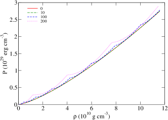
Figure 1: Matter contribution to the EoS (pressure $P$ vs mass density $\rho$) for a ¹²C WD, for different magnetic field strengths $b_{\star}$, where $b_{\star}=b/b_{\textrm{crit}}$ and $b_{\textrm{crit}}$ is defined in Eq. (6).

The magnetisation $\mathcal{M}$ is defined as:

$${\mathcal{M}}\equiv\left.\frac{\partial P}{\partial b}\right|_{\mu}\ .$$ (19)

In the recent work of Otoniel et al. (2016), nuclei are supposed to be arranged in a simple cubic lattice. However, such a structure is known to be unstable (Born, 1940). The baryon chemical potential $\mu$, which coincides with Gibbs free energy per nucleon

$$g=\frac{\mathcal{E}+P}{n}\ ,$$ (20)

is given by

$$\mu=\frac{M^{\prime}(A,Z)c^{2}}{A}+\frac{Z}{A}\left(\mu_{e}-m_{e}c^{2}+\mu_{L}\right)\ ,$$ (21)

where

$$\mu_{L}=\frac{4}{3}\frac{\mathcal{E}_{L}}{n_{e}}\ .$$ (22)

Complete general expressions of the magnetisation as well as of its derivatives can be found in Appendix A.

In the following, we shall consider stellar cores made of either ¹²C or ¹⁶O. These elements are the most likely fusion products of the helium burning phase.

3 Stellar structure equations

In this section, we outline the formalism to construct equilibrium WD configurations starting from the EoS described in Sec. 2. As general relativity has been shown to have a non-negligible effect on the maximum WD mass, we compute the structure of WDs within both Newtonian theory of gravity and the general relativistic framework, for comparison (see also Sec. 7.1). The matter properties enter the energy-momentum tensor which acts as a source of the Einstein equations. The equilibrium is determined by the conservation of energy and momentum, derived from the condition of vanishing divergence of the energy-momentum tensor. We then compute equilibrium numerical models of WDs to obtain the global structure properties such as mass or radius.

The Einstein-Maxwell and equilibrium equations described hereafter are solved using spectral methods within the numerical library lorene. We apply the numerical scheme originally designed for strongly magnetised neutron stars (see Chatterjee et al., 2015, for further details) to study strongly magnetised WD. As elaborated in Bocquet et al. (1995), the electromagnetic field tensor can be chosen to be either purely poloidal or purely toroidal. Within the numerical scheme of lorene, the magnetic field configuration is purely poloidal by construction. This is convenient for comparison with the observed surface poloidal fields as estimated from the spin-down measurements of pulsars. However, for neutron stars, it has been suggested that amplification of the seed poloidal magnetic field could result in the generation of strong toroidal fields. Following the same arguments, one may argue that the same holds for strongly magnetised WDs. Further, both purely poloidal and toroidal magnetic field configurations are unstable, resulting in the rearrangement of the configuration to a mixed one. That means, a purely poloidal magnetic field configuration is not necessarily the most general one. Studies of magnetised WDs in a general magnetic field configuration have been recently performed employing the XNS code (Bera & Bhattacharya, 2014, 2016; Das & Mukhopadhyay, 2015a). These studies showed that large WD masses can be supported by a purely toroidal field, but these configurations are also unstable. For the twisted torus mixed configuration (with a dominant poloidal field), the mass-radius relations obtained were similar to those of the purely poloidal case.

3.1 Energy-momentum tensor in presence of a magnetic field

In Chatterjee et al. (2015), some of us explicitly derived the generalised expression for the thermodynamic average of the microscopic energy-momentum tensor, which is required for the study of the macroscopic structure of a compact object, as recapitulated below:

$$\langle T^{\mu\nu}\rangle = (\mathcal{E}+P)\;u^{\mu}u^{\nu}+P\;g^{\mu\nu}$$ (23)

$$+\frac{1}{2}(F^{\nu}_{\;\tau}{\mathcal{M}}^{\tau\mu}+F^{\mu}_{\;\tau}{\mathcal{M}}^{\tau\nu})$$

$$-\frac{1}{\mu_{0}}(F^{\mu\alpha}F_{\alpha}^{\,\nu}+\frac{g^{\mu\nu}}{4}F_{\alpha\beta}F^{\alpha\beta})~{}.$$

where, $\mathcal{E}$ is the matter energy density, $P$ is the matter pressure (see Sec. 2), $u^{\mu}$ is the fluid four-velocity and $\mu_{0}$ is the vacuum magnetic permeability in S.I. units. The electromagnetic field strength tensor is derived from the electromagnetic potential 1-form $A_{\mu}$ through

$$F_{\mu\nu}=\frac{\partial A_{\nu}}{\partial x^{\mu}}-\frac{\partial A_{\mu}}{\partial x^{\nu}}\,,$$ (24)

and ${\mathcal{M}}^{\mu\nu}$ is the magnetisation tensor (see Chatterjee et al. (2015) for complete derivation).

The first two terms on the right hand side of (23) can be identified as the pure (perfect fluid) matter contribution, followed by the magnetisation term and finally the usual electromagnetic field contributions to the energy-momentum tensor. For isotropic media, the magnetisation is aligned with the magnetic field. Thus one may write $\displaystyle{\mathcal{M}}_{\alpha\beta}=\frac{\chi}{\mu_{0}}F_{\alpha\beta}$, in terms of the dimensionless scalar

$$\chi=\frac{\mu_{0}{\mathcal{M}}}{b}\,.$$ (25)

Finally, the electric and magnetic fields as measured by the Eulerian observer have only two non-vanishing components each (see Bonazzola et al., 1993):

$$E_{r} = \frac{1}{N}\left(\frac{\partial{A_{t}}}{\partial{r}}+N^{\varphi}\frac{\partial{A_{\varphi}}}{\partial{r}}\right),$$ (26a)

$$E_{\theta} = \frac{1}{N}\left(\frac{\partial{A_{t}}}{\partial{\theta}}+N^{\varphi}\frac{\partial{A_{\varphi}}}{\partial{\theta}}\right),$$ (26b)

$$B_{r} = \frac{1}{Cr^{2}\sin\theta}\frac{\partial{A_{\varphi}}}{\partial{\theta}},$$ (26c)

$$B_{\theta} = -\frac{1}{C\sin\theta}\frac{\partial{A_{\varphi}}}{\partial{r}},$$ (26d)

where $C,N$ and $N^{\varphi}$ are gravitational potentials defined by the metric (27). Note that we denote the magnetic field norm in the matter comoving frame by $b$, to distinguish it from that in the Eulerian frame, denoted by $B$ with components $B_{r}$ and $B_{\theta}$.

3.2 Einstein-Maxwell and equilibrium equations

To construct numerical models of magnetic WDs, we adapt the general relativitic scheme following previous works by Bocquet et al. (1995); Bonazzola et al. (1993). Under the assumptions of stationarity, axisymmetry and circularity of the spacetime, we employ the maximally sliced quasi-isotropic coordinates in which the line element can be written as:

$${\rm d}s^{2} = -N^{2}\,{\rm d}t^{2}+C^{2}r^{2}\sin^{2}\theta\left({\rm d}\varphi-N^{\varphi}\,{\rm d}t\right)^{2}$$ (27)

$$+D^{2}\left({\rm d}r^{2}+r^{2}\,{\rm d}\theta^{2}\right),$$

where $N,N^{\varphi},C$ and $D$ are functions of coordinates $(r,\theta)$. With these properties and coordinate choice, the Einstein equations reduce to a set of four elliptic partial differential equations for the four gravitational potentials, in which part of the source terms is derived from the energy-momentum tensor. These equations are then solved for a given matter content. Note that, in this section, Latin letters i, j, …are used for spatial indices only, whereas Greek ones $\alpha$, $\mu$, …denote the spacetime indices.

Whereas the homogeneous Maxwell equation is automatically verified by the expression (24) for the electromagnetic field tensor, the inhomogeneous one must be modified to include the contribution from the magnetisation (Chatterjee et al., 2015):

$$\frac{1}{\mu_{0}}\nabla_{\mu}F^{\nu\mu}=j_{\ \mathit{free}}^{\nu}+\nabla_{\mu}{\mathcal{M}}^{\nu\mu}~{},$$ (28)

where $j_{\ \mathit{free}}^{\nu}$ is the free current which generates the electromagnetic field, as opposed to the bound current contribution associated with the magnetisation (last term in the above equation). For a discussion about these free currents, which are not driven by the bulk motion of matter, see Bonazzola et al. (1993).

To obtain equilibrium configurations, one must solve the coupled Einstein-Maxwell equations, together with the condition of conservation of energy and momentum $\nabla_{\mu}T^{\mu\nu}=0$, giving rise to the equilibrium condition in our stationary case. It was already illustrated in Chatterjee et al. (2015) that on inclusion of the magnetisation current density in the equation of equilibrium, the Lorentz force associated with the magnetisation current cancels with the magnetisation contribution arising from the pressure gradient (key equations are recapitulated in the Appendix B). Therefore, there is no explicit magnetisation appearing in the equilibrium condition, and the first integral of fluid stationary motion remains unchanged retaining the same form as in the case without magnetisation (see details in App. B):

$$\ln h(r,\theta)+\nu(r,\theta)-\ln\Gamma(r,\theta)+\Phi(r,\theta)={\rm const},$$ (29)

where $h$ is the enthalpy (as we assume zero temperature, $h=g$ the Gibbs free energy, introduced in Eq. (20)), $\nu=\log N$ a gravitational potential function, $\Gamma$ is the Lorentz factor and $\Phi$ is the electromagnetic term associated with the Lorentz force (see Bonazzola et al., 1993, for a discussion):

$$\frac{\partial\Phi}{\partial x^{i}}=-\frac{F_{i\mu}j^{\mu}_{\ \mathit{free}}}{\mathcal{E}+P}.$$ (30)

3.3 Newtonian limit

As WDs are not strongly relativistic objects, their structure is often calculated in a non-relativistic Newtonian framework. We summarise here the basic stellar structure equations that the general relativistic equations reduce to in the Newtonian limit.

Whereas for Maxwell equations one must consider the special-relativistic form, the Newtonian limit of the Einstein equations is the Poisson equation for the gravitational potential $\phi$:

$$\nabla^{2}\phi=4\pi G\rho~{},$$ (31)

where $G$ is the gravitational constant and $\rho$ is the mass density. Thus in the non-relativistic limit, the factor $\nu$ tends to the Newtonian gravitational potential $\phi$ (Gourgoulhon, 2011).

The first integral of motion (Eq. 29), described in the previous section, reduces to a simple form in the Newtonian limit in the absence of an electromagnetic field

$$\hat{h}+\phi-\frac{1}{2}U^{2}={\rm const},$$ (32)

where $\hat{h}=\left(\hat{\mathcal{E}}+P\right)/\rho$ is the non-relativistic enthalpy (i.e. $\mathcal{E}=\rho\,c^{2}+\hat{\mathcal{E}}$, $\hat{\mathcal{E}}$ being the internal energy, not taking into account rest-mass energy density) and $U$ the fluid velocity in the $\varphi$-direction. Note here that, as shown, e.g., by Gourgoulhon (2011) this is not the classical Bernoulli equation, but a first integral of motion, which is valid only if the fluid is in pure circular motion, while the Bernoulli theorem is valid for any stationary flow. Moreover, the expression for the Bernoulli theorem provides a constant along each fluid line, which may vary from one fluid line to another, whereas the first integral (32) gives a constant valid in the entire star.

In presence of free currents $j^{\mu}_{\ \mathit{free}}$, see Eq. (28) and of the electromagnetic field they generate, a force term of the form $\displaystyle f_{i}=F_{i\sigma}j^{\sigma}_{\ \mathit{free}}$ is added to the equation of stationary motion (Bonazzola et al., 1993). Now, using the definition of $F_{\mu\nu}$ (24), together with the Newtonian limit (i.e. the metric potentials $N,C,D\to 1$ and $N^{\varphi}\to 0$) in Eqs. (26), and writing the 4-currents $j^{\mu}$ as a charge density $j^{0}_{\ \mathit{free}}$ and a current vector $\vec{j}_{\mathit{free}}$ separately, one gets the standard form for the force:

$$\vec{f}=j^{0}_{\ \mathit{free}}\,\vec{E}+\vec{\jmath}_{\mathit{free}}\times\vec{B}.$$ (33)

As we assume the matter inside the star to be a perfect conductor, we have the relation:

$$\vec{E}=-\vec{v}\times\vec{B},$$ (34)

with $\vec{v}=\Omega\,\vec{e}^{\varphi}$ the fluid velocity (thus, $U=\Omega r\sin\theta$) . The Newtonian interpretation of our requirement of having a first integral of motion, with the introduction of the potential $\Phi$ (30), is that the electromagnetic force be potential-like:

$$\vec{f}=\left(\vec{\jmath}-\Omega\,\vec{e}^{\varphi}j^{0}\right)\times\vec{B}=\rho\vec{\nabla}\Phi.$$ (35)

The equilibrium equation in the Newtonian case then reads:

$$\hat{h}+\phi-\frac{1}{2}U^{2}+\Phi=\textrm{const}.$$ (36)

As demonstrated before in the relativistic case, note again that the above equations for equilibrium do not contain any contribution from the magnetisation. They thus differ from those given in Bera & Bhattacharya (2014), where the magnetisation has been artificially included.

4 Stellar structure and magnetic field

With the numerical setup described in Sec. 3, we construct models of magnetic ¹²C WDs in equilibrium and determine their structure for various magnetic field strengths. After comparing our results with those obtained in previous studies, we show that the the relevant quantity to consider for assessing the global stability of strongly magnetised WDs is the magnetic dipole moment rather than the magnetic field strength. We compute the maximum mass and discuss the limitations of our model. Since the magnetic field dependence of the EoS is very weak, see the discussion in Sec. 6.1, we will neglect unless otherwise stated magnetisation and magnetic field dependence of the EoS for simplicity within the calculations.

4.1 Role of a strong magnetic field on the white dwarf structure

Based on a non-rotating model in Newtonian gravity, we first vary central enthalpy along sequences of fixed central magnetic fields $B_{\star}$ where $B_{\star}=B/b_{\textrm{crit}}$, $b_{\textrm{crit}}$ being defined in Eq. (6) and $B$ is the magnetic field measured by the Eulerian observer. The value remaining fixed along a given sequence corresponds to the value of magnetic field at the centre of the star. Indeed, for each choice of free current distribution (28) one obtains a given magnetic field distribution inside the star and thus one can determine the value of central magnetic field strength.

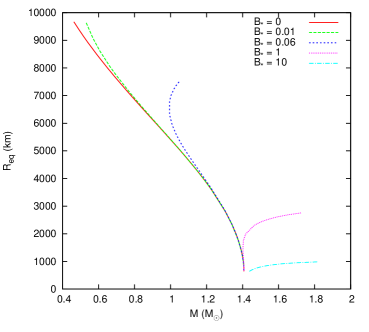
Figure 2: Masses $M$ in units of solar mass (M_⊙) as functions of equatorial radii $R_{eq}$ for ¹²C WDs in Newtonian gravity along 5 sequences of fixed central magnetic field $B_{\star}$, ranging from $0$ to $10$. $B_{\star}=B/b_{\textrm{crit}}$ and $b_{\textrm{crit}}$ is defined in Eq. (6).

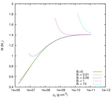
Figure 3: Masses $M$ in units of solar mass (M_⊙) as functions of central density $\rho_{c}$ for ¹²C WDs in Newtonian gravity along 5 sequences of fixed central magnetic fields $B_{\star}$, ranging from $0$ to $10$. $B_{\star}=B/b_{\textrm{crit}}$ and $b_{\textrm{crit}}$ is defined in Eq. (6).

Fig. 2 displays the mass $M$ (in units of solar mass M_⊙) as a function of equatorial radius $R_{eq}$ (in km) for such sequences in Newtonian gravity. For low magnetic fields, the sequences follow the mass-radius relation as for non-magnetic WDs, ultimately reaching the Chandrasekhar limit. As the field strength is increased, the deviation from the non-magnetic curve increases, resulting in configurations with higher mass at lower densities. This is clearly evident from Fig. 3, where for the same sequences we show the masses for varying central mass density $\rho_{c}$ (in g cm^-3). These results in Newtonian gravity are well known and can be compared with those of Suh & Mathews (2000); Bera & Bhattacharya (2014) and are found to be in accordance. For field strengths of about 10 $b_{\rm crit}$, masses as large as $\sim$ 1.8 M_⊙ are found to be supported by the magnetic field for both ¹²C and ¹⁶O.

These figures clearly demonstrate that WD masses larger than the standard Chandrasekhar limit for the non-magnetic case can be supported by strong magnetic fields. However, the strongly magnetised sequences ($B_{\star}=1,10$) seem to be gravitationally unstable, if one uses the standard criterion for non-magnetic stars $\partial R_{eq}/\partial M>0$ or $\partial M/\partial\rho_{c}<0$ (e.g. Shapiro & Teukolsky, 1983). The important point here is that, in order to look for such instabilities along families of two-parameter equilibria, one must be careful in choosing the quantity that should be kept constant when varying the mass (Sorkin, 1982). Indeed, just as in the case of a rotating body it is the angular momentum and not the angular velocity that is the constant of motion, it can be shown that the conservation of magnetic flux implies that magnetic moment is a constant of motion and not the magnetic field. Therefore, sequences of fixed dipole magnetic moments $\mathcal{D}$ should be considered, and not of fixed central magnetic field value as in Figs. 2 and 3. This dipole moment is computed from the asymptotic behaviour of the magnetic field, obtained from our numerical model (see Bocquet et al., 1995, for a definition).

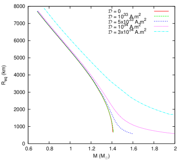
Figure 4: ¹²C WD masses $M$ vs radii $R_{eq}$ along sequences of fixed magnetic moments $\mathcal{D}$ in Newtonian gravity.

In Fig. 4 we therefore construct mass-radius relations for increasing central enthalpy along sequences of fixed dipole magnetic moments $\mathcal{D}$. As seen from this figure, even very highly-magnetised sequences, which can reach two solar masses configurations, are gravitationally stable in Newtonian gravity. Effects of relativistic gravity (General Relativity) shall be discussed later, in Sec. 7.1.

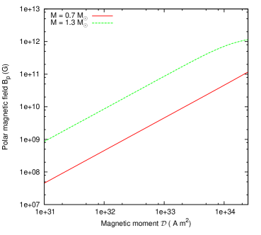
Figure 5: Polar magnetic field $B_{P}$ vs magnetic dipole moment $\mathcal{D}$ for ¹²C Newtonian WDs of baryon masses 0.7 $M_{\odot}$ and 1.3 $M_{\odot}$

Finally, as it is not the magnetic moment which is an astrophysically observable quantity, but rather the polar magnetic field which is derived from the measurement of the spin and spin periods, we here give relations between both quantities, so that one can get an idea of typical magnetic fields arising for the magnetic dipolar moments quoted in this study. For two exemplary typical values of WD masses (0.7 and 1.3 solar masses), we display in Fig. 5 the values of polar magnetic fields $B_{P}$ (in G) for a ¹²C WD corresponding to the range of magnetic moments considered in this work. One must here keep in mind that surface magnetic fields of isolated magnetic WDs are observed to lie within the range $10^{3}$ - $10^{9}$ G (Ferrario et al., 2015).

4.2 Maximally distorted stellar configurations

Figure 6: Enthalpy isocontours of a static stellar configuration in the $(x,z)$ plane of a ¹²C WD for a magnetic dipole moment of $3\times 10^{34}$ A m². The mass of the star is $1.99M_{\odot}$ and the polar magnetic field $B_{P}\sim 3\times 10^{13}$ G.

With stronger magnetic fields, the anisotropic Lorentz force acting on the free currents (33) causes the stellar structure to increasingly deviate from spherical symmetry, finally reaching a toroidal shape. At this point the code reaches the limit of its numerical capability for describing the stellar surface, and hence more massive stable WD configurations cannot be achieved within this numerical framework. As an example, in Fig. 6 we illustrate the maximally distorted shape of the stellar surface of a ¹²C WD for a magnetic dipole moment of $3\times 10^{34}$ A m². The induced magnetic field at the pole rises up to $3.1\times 10^{13}$ G (equivalently $B_{\star}\sim 1$) whereas the magnetic field at the centre reaches $B_{\star}\sim 10$. The ratio of magnetic to fluid pressure computed at the centre of the WD in this case is found to be $\sim 0.79$, and $0.83$ in the ¹⁶O EoS case. The endpoints of the curves for two-solar masses magnetised WDs in Fig. 4 correspond to these maximally distorted configurations, for which the numerical approach start being inaccurate. Strictly speaking, this does not represent an instability, and more massive stars with torus-like shape are not a priori excluded (see also the discussion in the case of neutron stars by Cardall et al., 2001). Nevertheless, it should be kept in mind that for these highly magnetised stars, the polar field is four orders of magnitude above the highest currently observed values and that, in particular, it is not clear in which way such a huge magnetic field could be formed within a WD. The stability of such toroidal stars has not been checked, either.

Another point is that we considered here a purely poloidal magnetic field configuration. Purely toroidal configurations might lead to much higher masses. However, it remains to be shown that these configurations are stable. In addition, under the fossil field hypothesis, the WD magnetic field is probably dominated by the poloidal field. As shown, e.g. in Bera & Bhattacharya (2016), the results for poloidal dominated mixed configurations are fairly similar to the results for purely poloidal fields discussed here. In Sec. 7 we will discuss other instabilities that may limit the mass of a magnetised WD.

5 Stellar structure and rotation

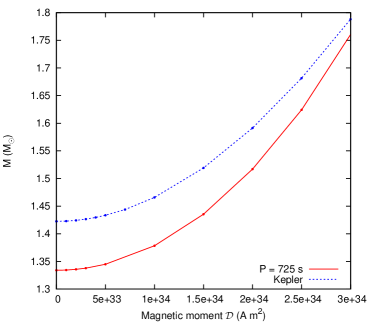
Figure 7: Masses for Newtonian magnetic WDs composed of ¹⁶O rotating with a period of 725 s (solid line) and at Kepler frequency (dashed line) as a function of fixed magnetic moments ${\mathcal{D}}$.

It is already a well known result that rotation provides centrifugal force that can support larger masses in compact stars. We estimated the relative increase in mass of a rotating magnetic WD compared to a non-rotating one. The observed rotation periods of isolated magnetic WDs span the range from 725 s to decades or centuries (Ferrario et al., 2015). Magnetic cataclysmic variables exhibit shorter periods, with AE Aqr having a period of 33 s. For such values of the rotation period, we find that the relative difference between the masses of non-rotating and rotating WDs at a given density and magnetic dipole moment is negligible (of the order of $10^{-4}$ or lower). On the contrary, the magnetic field plays a major role in supporting massive WDs. To demonstrate this fact, we display in Fig. 7 the maximum mass of a WD rotating with a period of 33 s (depicted by a solid line) - these results are indistinguishable from those obtained for a nonrotating WD - as well as a WD rotating at the Kepler frequency corresponding to the mass shedding limit (dashed line) for increasing values of the magnetic dipole moment. It is evident that even for the fastest rotating observed WDs, rigid rotation does not lead to any significant increase in their mass. More importantly, the effects of rotation are comparatively less important for strongly magnetised WDs, even at Kepler frequency, as the main force resisting gravity is no longer the centrifugal buoyancy, but the Lorentz force due to the magnetic field.

On the other hand, differentially rotating compact stars can be significantly more massive than their non-rotating or uniformly rotating counterparts (see, e.g., Subramanian & Mukhopadhyay, 2015). However, the support due to differential rotation would ultimately be cancelled by magnetic braking and/or viscosity. These processes drive the star into uniform rotation (Shapiro, 2000). As a matter of fact, Bonazzola et al. (1993) showed that a magnetic star in a stationary state is necessarily rigidly rotating.

6 Stellar structure and the equation of state

In this section, we perform a systematic analysis of the role of the EoS on the WD structure, and more specifically the effects of the magnetic field and electron-ion interactions.

6.1 Magnetic field dependence of the equation of state

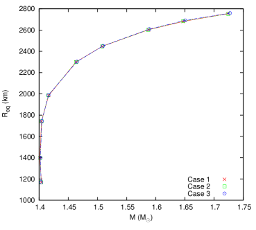
Figure 8: Radius $R_{eq}$ vs Mass $M$ for ¹²C Newtonian WDs for fixed central magnetic field $B_{c}=b_{\rm crit}$ (6), with and without magnetic field dependence in EoS and magnetisation. See text for details about the cases 1, 2 and 3.

As discussed in Section 2, the magnetic field influences the properties of dense matter in magnetic WDs through (i) Landau quantisation (i.e. magnetic-field dependent EoS), and (ii) the magnetisation $\mathcal{M}$. In order to assess the relative importance of these effects, we compute the structure of magnetic WDs for a fixed central magnetic field $B_{c}=b_{\rm crit}$ considering the three different cases:

• Case 1: EoS ignoring magnetic field effects,

• Case 2: EoS including Landau quantisation but neglecting magnetisation,

• Case 3: EoS including both Landau quantisation and magnetisation.

As shown Fig. 8, the corresponding mass-radius relationships are practically indistinguishable, in accordance with the results previously obtained by Bera & Bhattacharya (2014). Considering this result, Fig. 1, the discussion in Sec. 4.2 and the fact that the maximum values of the magnetic field inside the star remain low, only of the order of $B_{\star}\lesssim 10$, even for the maximally distorted configurations, we will adopt the simplest case 1 for the following calculations.

6.2 Electron-ion interactions

Most previous investigations of magnetic WDs have employed the EoS of an electron Fermi gas (Das & Mukhopadhyay, 2012a; Kundu & Mukhopadhyay, 2012; Bera & Bhattacharya, 2014; Das & Mukhopadhyay, 2015a; Franzon & Schramm, 2015). Bera & Bhattacharya (2016) and Otoniel et al. (2016) have recently computed the structure of magnetic WDs including the lattice correction to the EoS. Bera & Bhattacharya (2016) employed the expression obtained by Salpeter (1961) in the Wigner-Seitz approximation, while Otoniel et al. (2016) used the expression for a simple-cubic lattice. However, as already pointed out in Section 2, this lattice type is unstable. In all our calculations presented so far, (body-centred cubic) lattice corrections were taken into account. But in order to assess the importance of these effects, we now set $\mathcal{C}=0$, see Fig. 9, where the results without lattice effects are compared with the results taking them into account. We find that electron-ion interactions lead to a lower maximum mass for WDs, as previously discussed by Chamel & Fantina (2015) for non-magnetic WDs. However, the reduction is rather small: the maximum mass of ¹²C and ¹⁶O non-magnetic WDs thus decreases from $\sim$ 1.44 M_⊙ to $\sim$ 1.41 M_⊙. On the other hand, lattice effects can have a much larger impact on the stellar radius, up to about 50% for a non-magnetic star with a mass of 1.4 M_⊙. These effects are less pronounced in strongly magnetised WDs.

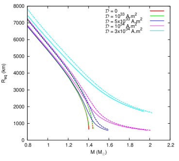
Figure 9: Mass-radius relations for Newtonian ¹⁶O WDs for different values of fixed magnetic moments with (solid lines) and without (dashed lines) lattice effects.

7 Stability of strongly magnetised white dwarfs

In this Section, we discuss several physical mechanisms that are able to affect the WD stability, turning some of the equilibrium solutions we have found so far into unstable ones. The aspects we consider here are the use of general relativity for the description of gravity; electron-capture instability and pycnonuclear instability. A summary of the different maximum mass values, considering the mechanisms discussed in this Section, can be found in Table 1 for ¹⁶O WDs and in Table 2 for ¹²C WDs.

7.1 General-relativistic instability

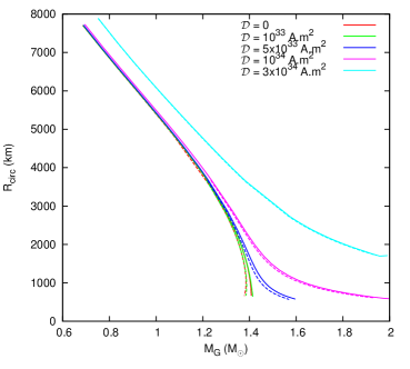
Figure 10: Circumferential radius $R_{circ}$ vs gravitational mass $M_{G}$ for magnetic ¹²C WDs along sequences of fixed magnetic dipole moments $\mathcal{D}$ in Newtonian theory (bold lines) and general relativity (dashed lines).

Although most mass-radius models for WDs have been constructed in Newtonian gravity, it is well known that computing equilibrium configurations within general relativity reduces the maximum mass for the case of non-magnetic WDs (e.g. Ibáñez (1983, 1984); Rotondo et al. (2011); Boshkayev et al. (2015)). We compute the structure of magnetised WDs both in Newtonian theory and in general relativity. To estimate how general relativistic effects may limit the maximum masses, we plot in Fig. 10 the mass-radius relationship for the non-magnetic as well as the magnetic WDs considering both Newtonian theory and general relativity. The mass used in general relativity is the so-called gravitational mass, which is the mass felt by a test-particle orbiting around the WD. For a complete definition, details of its computation and the definition of the circumferential equatorial radius used there too, see Bonazzola et al. (1993). It is clear from this figure that general relativity has a non-negligible effect in limiting the maximum mass of non-magnetic WD. We observed that on inclusion of general relativistic effects, the maximum mass of WD was reduced from the 1.41 M_⊙ to 1.38 M_⊙.

For the case of strongly magnetised WDs, it is found that it is not general relativity that plays a crucial role in limiting the maximum masses but the magnetic field which distorts the WD beyond the equilibrium poloidal shape. The reason is that general relativity affects the high-density part of the EoS, which determines the maximum mass for the non-magnetic case, but for the magnetic case it is rather the low-density part of the EoS which determines the maximum mass. To understand this we recall Fig. 3, where we plotted the masses as a function of density, from which it was evident that it is the low density part of the curves which bends away from the non-magnetic mass-radius relation and are responsible for the large masses, and the high density part remains unaffected. That the effect of general relativity on the maximum masses is small ($<2\%$ for poloidal fields) for the case of strongly magnetised WDs was demonstrated earlier by Das & Mukhopadhyay (2015a); Bera & Bhattacharya (2016) employing the XNS and LORENE codes.

7.2 Electron capture instability

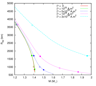
Figure 11: Mass radius relationship for magnetic WDs in Newtonian theory, composed of ¹²C along sequences of fixed magnetic moments including lattice effects in the EoS. The filled dots mark the onset of electron capture on ¹²C nuclei and the threshold electron capture densities for daughter nucleus obtained from pycnonuclear reactions are marked with filled squares. The corresponding onset for ¹⁶O WDs are shown by open symbols. The mass-radius relationship for ¹⁶ O WDs is not shown since the difference to ¹²C is maximally a few percent, hardly visible on the figure.

Chamel et al. (2013) pointed out that the onset of electron captures by nuclei (with the emission of a neutrino),

$$^{A}_{Z}X+e^{-}\rightarrow^{A}_{Z-1}Y+\nu_{e}\,,$$ (37)

may induce a local instability in magnetic WDs thus limiting their maximum gravitational mass. In the absence of magnetic fields, the onset of electron captures occur at mass density $\rho_{\beta}\simeq 4.16\times 10^{10}$ g cm^-3 (pressure $P_{\beta}\simeq 6.99\times 10^{28}$ dyn cm^-2) for ¹²C and $\rho_{\beta}\simeq 2.06\times 10^{10}$ g cm^-3 ($P_{\beta}\simeq 2.73\times 10^{28}$ dyn cm^-2) for ¹⁶O (Chamel & Fantina, 2015). In the presence of a strong magnetic field, the threshold density and pressure are shifted to either higher or lower values depending on the magnetic field strength (Chamel & Fantina, 2015), an effect which has been neglected until recently. Otoniel et al. (2016) have considered two limiting cases: (i) the absence of magnetic field, and (ii) the presence of a strongly quantising magnetic field such that only the lowest Landau level is filled and $\rho_{\beta}=\rho_{\rm b}$. In both cases, Otoniel et al. (2016) neglected the effects of electron-ion interactions on $\rho_{\beta}$, as in the study of Bera & Bhattacharya (2016). In the present work, we take into account the full dependence of the threshold density $\rho_{\beta}$ on the magnetic field strength including lattice corrections, as computed by Chamel & Fantina (2015). In this way, both the EoS and the electron capture threshold are calculated fully consistently.

The resulting mass-radius relations and electron capture thresholds for magnetic WDs along fixed magnetic moment sequences are shown in Fig. 11 considering stars made of either ¹²C or ¹⁶O. The filled and open dots along the sequences indicate the onset of electron capture instability for ¹²C and ¹⁶O respectively. The mass-radius relations for ¹⁶O differ only marginally from those obtained for ¹²C, and are not displayed on the figure for better readability. Our calculations confirm the suggestion of Chamel et al. (2013, 2014) that the electron capture instability can be a limiting factor for determining the maximum WD mass and in turn the maximum magnetic field. For magnetic moments as large as $10^{34}$ A.m², electron capture instability (in the case with lattice) limits the maximum gravitational mass to 1.86 M_⊙ for ¹²C. For ¹⁶O, the onset of the instability is reached at even lower values of the magnetic field, thus leading to a maximum gravitational mass of 1.67 M_⊙. This can be clearly understood from Fig. 1 of Chamel & Fantina (2015), where the onset of electron capture instability was shown to occur at lower densities for ¹⁶O than for ¹²C. For higher magnetic moments, the star becomes maximally distorted before the electron capture threshold is reached. In this case, the maximum gravitational mass could thus be potentially higher than that shown in Fig. 11, see also Otoniel et al. (2016). Fig. 12 shows the mass of ¹⁶O WDs as a function of the core magnetic field strengths for different fixed magnetic dipole moments. Here we show again the onset of electron capture instabilities by open dots along the curves. It is evident from the figure that the higher the magnetic moment is, the larger is the increase of the mass with the core magnetic field strength. All in all, no stellar configurations with a poloidal magnetic field are found with a mass above 2 M_⊙, if the star is not allowed to take a toroidal shape.

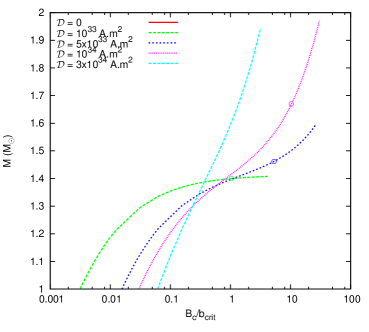
Figure 12: Central magnetic field $B_{c}$, in units of $b_{\rm crit}$ (6), vs WD mass $M$ for different fixed magnetic moments $\mathcal{D}$ for Newtonian ¹⁶O WDs. The open dots show the onset of electron capture.

Table 1: Maximum masses (in M_⊙) of strongly magnetised ¹⁶O WDs for various magnetic moments (in A.m²), limited by different mechanisms: B denotes the onset of torus-like shape due to magnetic field, EC stands for electron capture instability, pycno is short for pycnonuclear fusion reactions.

Magnetic moment		16O, without lattice			16O, with lattice
(A.m2)	B	B+EC	B+pycno	B	B+EC	B+pycno
0	1.44	1.44	1.25	1.40	1.40	1.21
$10^{33}$	1.45	1.44	1.25	1.41	1.40	1.21
$5\times 10^{33}$	1.60	1.50	1.25	1.59	1.46	1.22
$10^{34}$	2.01	1.68	1.26	1.97	1.67	1.23
$3\times 10^{34}$	1.96	1.96	1.40	1.94	1.94	1.38

Table 2: Maximum masses (in M_⊙) of strongly magnetised ¹²C WDs for various magnetic moments (in A.m²), limited by different mechanisms: B denotes the onset of torus-like shape due to magnetic field, EC stands for electron capture instability, pycno is short for pycnonuclear fusion reactions.

Magnetic moment		12C, without lattice			12C, with lattice
(A.m2)	B	B+EC	B+pycno	B	B+EC	B+pycno
0	1.44	1.44	1.41	1.41	1.41	1.38
$10^{33}$	1.45	1.44	1.41	1.41	1.41	1.38
$5\times 10^{33}$	1.60	1.528	1.43	1.60	1.50	1.40
$10^{34}$	2.01	1.85	1.48	2.00	1.86	1.47
$3\times 10^{34}$	2.03	2.03	2.03	1.96	1.96	1.96

7.3 Pycnonuclear instability

As first discussed by Chamel et al. (2013), pycnonuclear fusion reactions, whereby nuclei transform as

$$^{A}_{Z}X+^{A}_{Z}X\to^{2A}_{2Z}Y\,,$$ (38)

could play an important role in limiting the masses of strongly magnetised WDs. However, the rates of these processes remain highly uncertain (Yakovlev et al., 2006). We can estimate the strongest impact on the maximum mass by considering that pycnonuclear reactions set in at densities below the threshold density $\rho_{\beta}$ for the onset of electron capture by the daughter nuclei ${}^{2A}_{2Z}Y$. From Table I of Chamel & Fantina (2015), it is evident that the daughter nucleus ${}^{2A}_{2Z}Y$ is generally much more unstable than the parent nucleus ${}^{A}_{Z}X$ (e.g. the threshold density $\rho_{\beta}$ for ³²S is $1.69\times 10^{8}$ g/cm³ while that of ¹⁶O is $2.06\times 10^{10}$ g/cm³, including lattice effects). In Fig. 11, we mark the threshold densities $\rho_{\beta}$ for the daughter nucleus ³²S (from the fusion of ¹⁶O) and ²⁴ Mg (from the fusion of ¹²C), respectively, with empty and open squares along the curve. We find that for the non-magnetic case, the maximum mass decreases from 1.40 M_⊙ to 1.21 M_⊙ for ¹⁶O. Excluding lattice interactions increases both masses by about 3%. The effect is much less pronounced for ¹²C, where the threshold density is higher. Here the maximum mass in the non-magnetised case becomes $1.38M_{\odot}$. This is in agreement with the results quoted in Chamel & Fantina (2015). In the presence of a strongly quantizing magnetic field, the reduction of the maximum mass of WDs is even more spectacular: for a magnetic moment of $10^{34}$ A m², the maximum mass decreases from 1.97 M_⊙ to 1.23 M_⊙ for ¹⁶O WDs. Because pycnonuclear reactions may actually occur at densities above the electron capture threshold density for the daughter nuclei, the values we found for the maximum mass represent lower bounds.

8 Gravitational wave emission

It was conjectured by Heyl (2000) that rotating magnetic WDs could be important sources of gravitational waves (GW) detectable by the proposed eLISA mission (Evolved Laser Interferometer Space Antenna). Heyl estimated the GW emission for a number of observed rotating magnetic WDs using simple approximations for the reduced quadrupole moment. Using the analytic prescription of Bonazzola & Gourgoulhon (1996), where the distortion due to the magnetic field and due to rotation are assumed to be decoupled, we calculated the gravitational wave amplitudes for the potential sources listed in Table 1 of Heyl (2000). We numerically estimated the quadrupole moment in a self-consistent way within our improved microscopic model, assuming a gravitational mass of $0.6M_{\odot}$ and an internal magnetic field of $10^{11}$ G. We obtained a lower value of $0.58\times 10^{46}$ g cm² for quadrupole moment, close to the value $10^{47}$ g cm² obtained in Heyl (2000). However, although the discussion in Heyl (2000) concluded that the amplitude was within the detectable range of the former LISA interferometer project, our calculations of gravitational wave amplitudes for the rotating magnetic WDs estimated here are not likely to be detectable by the current project eLISA, as they are not within the estimated sensitivity range.

9 Conclusions

Using the formalism developed by Chatterjee et al. (2015), we have studied the equilibrium structure of WDs endowed with a strong poloidal magnetic field focusing on the determination of the maximum mass. In our approach, the coupled equilibrium equations for magnetic and gravitational fields are solved taking consistently into account stellar deformations due to rotations and/or anisotropies introduced by the magnetic field.

For our investigation, we have employed both general relativity and Newtonian theory for the description of gravity, together with the EoS of a degenerate electron Fermi gas interacting with a pure ionic crystal lattice made of ¹²C or ¹⁶O. The magnetic-field dependence of the EoS induced by Landau quantisation of electron motion has been fully included, as well as the resulting magnetisation of stellar matter. However, our numerical calculations have demonstrated that neither of these effects does significantly alter the structure of magnetised WDs, and they can thus be neglected. Still, the magnetic field can have a large impact on the stellar mass and radius. In particular, stellar configurations more massive than the standard Chandrasekhar limit can be obtained for magnetic field strengths higher than the critical value $b_{\rm crit}\sim 4.4\times 10^{13}$ G, as found in previous works. We have also examined more closely the role of electron-ion interactions, which have been often neglected in previous studies of strongly magnetised WDs. Because these interactions are attractive, the maximum mass is reduced by a few percent. On the other hand, the stellar radius can be increased by up to $\sim 50\%$ for nonmagnetic WDs with a mass of 1.4 M_⊙, and therefore these interactions should be included in any realistic model of WDs.

To explore whether strongly magnetised WDs are globally stable, we have performed calculations of sequences of equilibrium stellar configurations along fixed values of the magnetic dipole moment. We have found that the presence of a strong magnetic field can lead to large deformations of the star. For high enough values of the magnetic dipole moment, the stellar shape thus becomes toroidal. This extreme configuration is reached for gravitational masses below $2M_{\odot}$ and a surface magnetic field of the order of $10^{13}$-$10^{14}$ G. Note that, with our models of poloidal magnetic field the core magnetic strength is about one order of magnitude higher than the surface one. More strongly magnetised stellar configurations cannot be treated within our numerical framework, as the star gets a torus-like shape (magnetic pressure becomes larger than fluid pressure in the centre). We have also investigated the role of rotation on the stellar structure, and we have found that the maximum mass of magnetic WDs is increased by a few percent at most, the effects being the largest in the absence of magnetic fields.

Although torus-shaped strongly magnetised WDs with a mass above 2 M_⊙ could potentially exist beyond the distorted configurations computed in the present work, various instabilities can arise. First of all, it is well-known that general relativity can limit the maximum mass of nonmagnetic WDs. We have thus computed the structure of strongly magnetised WDs in full general relativity and have found that for weakly magnetised WDs, general relativistic effects reduce the maximum mass, as already discussed by De-Hua et al (2014); Coelho et al. (2014); Bera & Bhattacharya (2016). On the other hand, general relativity hardly plays any role in limiting the masses of strongly magnetised WDs, as anticipated by Kundu & Mukhopadhyay (2012). More importantly, the stability of strongly magnetised WDs is found to be mainly limited by the onset of electron capture and pycnonuclear reactions in the stellar core, as argued by Chamel et al. (2013). We have determined the threshold densities and pressures consistently with the EoS, including for the first time the effects due to both electron-ion interactions and the magnetic field. Given the high uncertainties on the pycnonuclear fusion reaction rates, we have estimated the maximum possible reduction of the WD mass by assuming that these processes set in at the same threshold density and pressure as electron captures by the daughter nuclei. These reactions lead to a drastic decrease in the maximum WD mass to values even below the Chandrasekhar limit. Our numerical results about mass limits are summarized in Tables 1 and 2. Additionally, we have estimated gravitational wave amplitudes emitted from rotating magnetised WDs, for which the magnetic and rotation axes are misaligned. We come to the conclusion that, from the currently observed WDs, none could be detected by the future space-based gravitational-wave detector eLISA.

Extremely-magnetised WDs can thus in principle reach masses higher than $2\ M_{\odot}$ and remain stable with respect to gravitational and electron capture instabilities; the consequence being that they would have torus-like shapes. On the other hand, pycnonuclear instablities could severely limit the existence of such stars, but one must keep in mind the high uncertainties associated with these reactions. In summary, the possibility of super-Chandrasekhar strongly magnetised WDs cannot be totally excluded from current theoretical considerations, but important issues still need to be addressed before any firm conclusions on their existence could be drawn. First, the dynamical stability of these extremely high magnetic fields in such cold dense crystallized stellar environment remains to be proved. Moreover, the magnetic field strengths expected at the surface of such strongly magnetised WDs appear to be four orders of magnitude higher than the upper limit of about $10^{9}$ G set by currently observed magnetic WDs. Finally, no realistic and quantitative astrophysical formation scenarios have been so far proposed to explain the origin of such strongly magnetised WDs.

Appendix A General expression for the magnetization

We report here for completeness and future reference the general expressions for the magnetization and its first derivative, that are needed with the EoS to compute the WD structure. Starting from the definition of $\mathcal{M}\equiv\partial P/\partial b|_{\mu}$, Eq. (19), we first observe that constant chemical potential implies:

$$d\mu=0\Longrightarrow d\mu_{e}=-d\mu_{L}\ ,$$ (39)

where we have used Eqs. (21) and (22). Writing explicitly the dependence of the pressure on the magnetic field $b$ and the electron chemical potential $\mu_{e}$ as $P=P(b,\mu_{e})$, we obtain:

$$\mathcal{M}\equiv\left.\frac{\partial P}{\partial b}\right|_{\mu}=\left.\frac{\partial P}{\partial b}\right|_{\mu_{e}}-\left.\frac{\partial P}{\partial\mu_{e}}\right|_{b}\left.\frac{\partial\mu_{L}}{\partial b}\right|_{\mu_{e}}\left[1+\left.\frac{\partial\mu_{L}}{\partial\mu_{e}}\right|_{b}\right]^{-1}\ ,$$ (40)

with

$$\frac{\partial P}{\partial b}=\frac{\partial P_{L}}{\partial b}+\frac{\partial P_{e}}{\partial b}\ ,$$ (41)

$$\frac{\partial P}{\partial\mu_{e}}=\frac{\partial P_{L}}{\partial\mu_{e}}+\frac{\partial P_{e}}{\partial\mu_{e}}\ .$$ (42)

Using the definition of $b_{\rm crit}$ and $\gamma_{e}$ from Eqs. (6) and (9), we also note that:

$$\frac{\partial}{\partial b}=\frac{1}{b_{\rm crit}}\frac{\partial}{\partial b_{\star}}\ ,$$ (43)

$$\frac{\partial}{\partial\mu_{e}}=\frac{1}{m_{e}c^{2}}\frac{\partial}{\partial\gamma_{e}}\ .$$ (44)

We thus find for the first derivative of the pressure (lattice and electron contribution) with respect to $b$:

$$\left.\frac{\partial P_{L}}{\partial b}\right|_{\mu_{e}}=\frac{4}{9}\frac{\mathcal{C}e^{2}}{b_{\rm crit}}Z^{2/3}n_{e}^{1/3}\left.\frac{\partial n_{e}}{\partial b_{\star}}\right|_{\gamma_{e}}\ ,$$ (45)

with:

$$\left.\frac{\partial n_{e}}{\partial b_{\star}}\right|_{\gamma_{e}}=\frac{n_{e}}{b_{\star}}+\frac{2b_{\star}}{(2\pi)^{2}\lambda_{e}^{3}}\sum_{\nu_{L}=0}^{\nu_{L}^{\rm max}}g_{\nu}\frac{\partial x_{e}}{\partial b_{\star}}\ ,$$ (46)

$$\frac{\partial x_{e}}{\partial b_{\star}}=-\frac{\nu_{L}}{x_{e}}\ ;$$ (47)

$$\left.\frac{\partial P_{e}}{\partial b}\right|_{\mu_{e}} = \frac{P_{e}}{b}$$

$$-\frac{b_{\star}m_{e}c^{2}}{(2\pi)^{2}\lambda_{e}^{3}b_{\rm crit}} \times \sum_{\nu_{L}=0}^{\nu_{L}^{\rm max}}2g_{\nu}\nu_{L}\ln\left(\frac{\gamma_{e}+x_{e}}{\sqrt{1+2\nu_{L}b_{\star}}}\right)\ .$$ (48)

For the first derivative of the pressure (lattice and electron contribution) with respect to $\mu_{e}$, we find:

$$\left.\frac{\partial P_{L}}{\partial\mu_{e}}\right|_{b}=\frac{4}{9}\frac{\mathcal{C}e^{2}}{m_{e}c^{2}}Z^{2/3}n_{e}^{1/3}\left.\frac{\partial n_{e}}{\partial\gamma_{e}}\right|_{b_{\star}}\ ,$$ (49)

with:

$$\left.\frac{\partial n_{e}}{\partial\gamma_{e}}\right|_{b_{\star}}=\frac{2b_{\star}}{(2\pi)^{2}\lambda_{e}^{3}}\sum_{\nu_{L}=0}^{\nu_{L}^{\rm max}}g_{\nu}\frac{\partial x_{e}}{\partial\gamma_{e}}\ ,$$ (50)

$$\frac{\partial x_{e}}{\partial\gamma_{e}}=\frac{\gamma_{e}}{x_{e}}\ ;$$ (51)

$$\left.\frac{\partial P_{e}}{\partial\mu_{e}}\right|_{b}=\frac{b_{\star}}{(2\pi)^{2}\lambda_{e}^{3}}\sum_{\nu_{L}=0}^{\nu_{L}^{\rm max}}2g_{\nu}x_{e}=n_{e}\ .$$ (52)

The first derivatives of the chemical potential can be written as:

$$\left.\frac{\partial\mu_{L}}{\partial b}\right|_{\mu_{e}}=\frac{4}{9}\frac{\mathcal{C}e^{2}}{b_{\rm crit}}Z^{2/3}n_{e}^{-2/3}\left.\frac{\partial n_{e}}{\partial b_{\star}}\right|_{\gamma_{e}}\ ,$$ (53)

using Eq. (46), and

$$\left.\frac{\partial\mu_{L}}{\partial\mu_{e}}\right|_{b}=\frac{4}{9}\frac{\mathcal{C}e^{2}}{m_{e}c^{2}}Z^{2/3}n_{e}^{-2/3}\left.\frac{\partial n_{e}}{\partial\gamma_{e}}\right|_{b_{\star}}\ ,$$ (54)

using Eq. (50).

To calculate the derivative of $M$,

$$\frac{\partial\mathcal{M}}{\partial\mu}=\frac{\partial^{2}P}{d\mu\partial b}=\left.\frac{\partial\mathcal{M}}{\partial\mu_{e}}\right|_{b}\left(\left.\frac{\partial\mu}{\partial\mu_{e}}\right|_{b}\right)^{-1}\ ,$$ (55)

we write explicitly the terms appearing in Eq. (55) as:

$$\left.\frac{\partial\mathcal{M}}{\partial\mu_{e}}\right|_{b} = \frac{1}{m_{e}c^{2}}\left\{\frac{\partial}{\partial\gamma_{e}}\left.\frac{\partial P}{\partial b}\right|_{\mu_{e}}\right.$$ (56)

$$- \left.\frac{\partial}{\partial\gamma_{e}}\left(\left.\frac{\partial P}{\partial\mu_{e}}\right|_{b_{\star}}\right)\left.\frac{\partial\mu_{L}}{\partial b}\right|_{\mu_{e}}\left(1+\left.\frac{\partial\mu_{L}}{\partial\mu_{e}}\right|_{b}\right)^{-1}\right.$$

$$- \left.\left.\frac{\partial P}{\partial\mu_{e}}\right|_{b_{\star}}\frac{\partial}{\partial\gamma_{e}}\left(\left.\frac{\partial\mu_{L}}{\partial b}\right|_{\mu_{e}}\right)\left(1+\left.\frac{\partial\mu_{L}}{\partial\mu_{e}}\right|_{b}\right)^{-1}\right.$$

$$+ \left.\left.\frac{\partial P}{\partial\mu_{e}}\right|_{b_{\star}}\left.\frac{\partial\mu_{L}}{\partial b}\right|_{\mu_{e}}\left(1+\left.\frac{\partial\mu_{L}}{\partial\mu_{e}}\right|_{b}\right)^{-2}\right.$$

$$\times \left.\frac{\partial}{\partial\gamma_{e}}\left(\left.\frac{\partial\mu_{L}}{\partial\mu_{e}}\right|_{b_{\star}}\right)\right\}\ ,$$

and

$$\left.\frac{\partial\mu}{\partial\mu_{e}}\right|_{b}=y_{e}\left(1+\left.\frac{\partial\mu_{L}}{\partial\mu_{e}}\right|_{b}\right)\ ,$$ (57)

where each contribution of the pressure derivative can be calculated according to Eqs. (41)-(42). We thus obtain, for the second derivative of the pressure (electron and lattice contribution):

$$\frac{\partial}{\partial\gamma_{e}}\left(\left.\frac{\partial P_{L}}{\partial b}\right|_{\mu_{e}}\right)_{b_{\star}}\mkern-18.0mu = \frac{4}{9}\frac{\mathcal{C}e^{2}}{b_{\rm crit}}Z^{2/3}\left[\frac{1}{3}n_{e}^{-2/3}\left.\frac{\partial n_{e}}{\partial\gamma_{e}}\right|_{b_{\star}}\left.\frac{\partial n_{e}}{db_{\star}}\right|_{\gamma_{e}}\right.$$ (58)

$$+ \left.n_{e}^{1/3}\frac{\partial}{\partial\gamma_{e}}\left.\left(\frac{\partial n_{e}}{\partial b_{\star}}\right)\right|_{b_{\star}}\right]\ ,$$

using Eqs. (46) and (50), and

$$\frac{\partial}{\partial\gamma_{e}}\left(\left.\frac{\partial n_{e}}{\partial b_{\star}}\right|_{\mu_{e}}\right)_{b_{\star}} = \frac{2}{(2\pi)^{2}\lambda_{e}^{3}}\sum_{\nu_{L}=0}^{\nu_{L}^{\rm max}}g_{\nu}\frac{\partial x_{e}}{\partial\gamma_{e}}$$ (59)

$$+ \frac{2b_{\star}}{(2\pi)^{2}\lambda_{e}^{3}}\sum_{\nu_{L}=0}^{\nu_{L}^{\rm max}}g_{\nu}\frac{\partial}{\partial\gamma_{e}}\left(\frac{\partial x_{e}}{\partial b_{\star}}\right)\ ,$$

with $\partial x_{e}/\partial\gamma_{e}$ from Eq. (51) and

$$\frac{\partial}{\partial\gamma_{e}}\left(\frac{\partial x_{e}}{\partial b_{\star}}\right)=\frac{\nu_{L}\ \gamma_{e}}{x_{e}^{3}}\ ;$$ (60)

$$\frac{\partial}{\partial\gamma_{e}}\left(\left.\frac{\partial P_{e}}{\partial b}\right|_{\mu_{e}}\right)_{b_{\star}}=\frac{n_{e}m_{e}c^{2}}{b}-\frac{b_{\star}m_{e}c^{2}}{(2\pi)^{2}\lambda_{e}^{3}b_{\rm crit}}\sum_{\nu_{L}=0}^{\nu_{L}^{\rm max}}2\frac{g_{\nu}\nu_{L}}{x_{e}}\ ;$$ (61)

$$\frac{\partial}{\partial\gamma_{e}}\left(\left.\frac{\partial P_{L}}{\partial\mu_{e}}\right|_{b_{\star}}\right)_{b_{\star}} = \frac{4}{9}\frac{\mathcal{C}e^{2}}{m_{e}c^{2}}Z^{2/3}\left[\frac{1}{3}n_{e}^{-2/3}\left(\left.\frac{\partial n_{e}}{\partial\gamma_{e}}\right|_{b_{\star}}\right)^{2}\right.$$ (62)

$$+ \left.n_{e}^{1/3}\frac{\partial}{\partial\gamma_{e}}\left(\left.\frac{\partial n_{e}}{\partial\gamma_{e}}\right|_{b_{\star}}\right)\right]\ ,$$

using Eq. (50) and:

$$\frac{\partial}{\partial\gamma_{e}}\left(\left.\frac{\partial n_{e}}{\partial\gamma_{e}}\right|_{b_{\star}}\right)_{b_{\star}}=\frac{2b_{\star}}{(2\pi)^{2}\lambda_{e}^{3}}\sum_{\nu_{L}=0}^{\nu_{L}^{\rm max}}g_{\nu}\frac{\partial}{\partial\gamma_{e}}\left(\frac{\partial x_{e}}{\partial\gamma_{e}}\right)\ ,$$ (63)

with:

$$\frac{\partial}{\partial\gamma_{e}}\left(\frac{\partial x_{e}}{\partial\gamma_{e}}\right)=-\frac{1+2\nu_{L}b_{\star}}{x_{e}^{3}}\ ;$$ (64)

$$\frac{\partial}{\partial\gamma_{e}}\left(\left.\frac{\partial P_{e}}{\partial\mu_{e}}\right|_{b_{\star}}\right)_{b_{\star}}=\frac{2b_{\star}}{(2\pi)^{2}\lambda_{e}^{3}}\sum_{\nu_{L}=0}^{\nu_{L}^{\rm max}}\frac{g_{\nu}\ \gamma_{e}}{x_{e}}\ .$$ (65)

For the second derivatives of the chemical potential, we have:

$$\frac{\partial}{\partial\gamma_{e}}\left(\left.\frac{\partial\mu_{L}}{\partial b}\right|_{\mu_{e}}\right)_{b_{\star}} = \frac{4}{9}\frac{\mathcal{C}e^{2}}{b_{\rm crit}}Z^{2/3}$$ (66)

$$\times \left[-\frac{2}{3}n_{e}^{-5/3}\left(\left.\frac{\partial n_{e}}{\partial\gamma_{e}}\right|_{b_{\star}}\right)\left(\left.\frac{\partial n_{e}}{\partial b_{\star}}\right|_{\mu_{e}}\right)\right.$$

$$+ \left.n_{e}^{-2/3}\frac{\partial}{\partial\gamma_{e}}\left(\left.\frac{\partial n_{e}}{\partial b_{\star}}\right|_{\mu_{e}}\right)_{b_{\star}}\right]\ ,$$

where we have used Eqs. (50) and (59), and

$$\frac{\partial}{\partial\gamma_{e}}\left(\left.\left(\frac{\partial\mu_{L}}{\partial\mu_{e}}\right)\right|_{b_{\star}}\right)_{b_{\star}} = \frac{4}{9}\frac{\mathcal{C}e^{2}}{m_{e}c^{2}}Z^{2/3}$$ (67)

$$\times \left[-\frac{2}{3}n_{e}^{-5/3}\left(\left.\frac{\partial n_{e}}{\partial\gamma_{e}}\right|_{b_{\star}}\right)^{2}\right.$$

$$+ \left.n_{e}^{-2/3}\frac{\partial}{\partial\gamma_{e}}\left(\left.\frac{\partial n_{e}}{\partial\gamma_{e}}\right|_{b_{\star}}\right)_{b_{\star}}\right]\ ,$$

where we made use of Eqs. (50) and (63).

Appendix B Derivation of the first integral in general relativity

The constraint for the conservation of energy and momentum in equilibrium can is expressed as :

$$\nabla_{\mu}T^{\mu\nu}=0.$$ (68)

Inserting the expression for the energy momentum tensor as in Eq.(23) into the above equation yields (Chatterjee et al., 2015)

$$(\mathcal{E}+P)\left(\frac{1}{\mathcal{E}+P}\frac{\partial P}{\partial x^{i}}+\frac{\partial\nu}{\partial x^{i}}-\frac{\partial\ln\Gamma}{\partial x^{i}}\right)$$

$$-F_{i\rho}j^{\rho}_{\ \mathit{free}}-\frac{\chi}{2\mu_{0}}F_{\mu\nu}\nabla_{i}F^{\mu\nu} = 0~{}.$$ (69)

where one can identify the first part as the perfect-fluid contribution to the energy-momentum tensor and the Lorentz force terms arising from free currents and the magnetization. Defining the enthalpy as a function of both baryon density and magnetic field norm $b=\sqrt{b^{\mu}b_{\mu}}$ in the comoving frame:

$$h=h(n,b)=\frac{\mathcal{E}+P}{m_{B}nc^{2}}~{},$$ (70)

where $m_{B}$ is the mean mass of a baryon. One can rewrite the first term in the parentheses of Eq. (69) in terms of the enthalpy as

$$\frac{\partial P}{\partial x^{i}}=(\mathcal{E}+P)\frac{\partial\ln h}{\partial x^{i}}+\mathcal{M}\frac{\partial b}{\partial x^{i}}\,.$$ (71)

The magnetic field in the comoving frame $b^{\mu}$ is defined by

$$F_{\mu\nu}=\epsilon_{\alpha\beta\mu\nu}u^{\beta}b^{\alpha}$$ (72)

and

$${\mathcal{M}}_{\mu\nu}=\epsilon_{\alpha\beta\mu\nu}u^{\beta}\mathcal{M}^{\alpha}.$$ (73)

Further, the last term in Eq. (69) can be written in terms of the magnetic field $b^{\mu}$ in the comoving frame as :

$$\frac{\chi}{2\mu_{0}}F_{\mu\nu}\nabla_{i}F^{\mu\nu} = \frac{\chi}{\mu_{0}}b_{\mu}\nabla_{i}b^{\mu}-b_{\mu}b^{\mu}u_{\nu}\nabla_{i}u^{\nu}$$ (74)

$$= b\nabla_{i}b=\mathcal{M}\frac{\partial{b}}{\partial{x^{i}}}.$$

Thus, inserting Eqs. (71) and (74) into Eq. (69), one gets an expression without explicit dependence on magnetization

$$\frac{\partial\ln h}{\partial x^{i}}+\frac{\partial\nu}{\partial x^{i}}-\frac{\partial\ln\Gamma}{\partial x^{i}}-\frac{F_{i\rho}j^{\rho}_{\ \mathit{free}}}{\mathcal{E}+P}=0,$$ (75)

which has the same form as in absence of magnetization (Bonazzola et al., 1993; Bocquet et al., 1995). Finally, as in Chatterjee et al. (2015) we introduce the current function, whose primitive is noted $\Phi(r,\theta)$ and defined by Eq. (30). This enables us to get a first integral of motion as given in Eq. (29).

References

- Adam (1986) Adam D., 1986, A&A, 160, 95
- Audi et al. (2012) Audi G., Wang M., Wapstra A. H., Kondev F. G., MacCormick M., Xu X., Pfeiffer B., 2012, Chin. Phys. C, 36, 1287
- Baiko et al. (2001) Baiko D. A., Potekhin A. Y., Yakovlev D. G., 2001, Phys. Rev. E, 64, 057402
- Baiko (2009) Baiko D. A., 2009, Phys. Rev. E, 80, 046405
- Belyaev et al. (2015) Belyaev V. B., Ricci P., Šimkovic F., Adam J. and Truhlík E., 2015, Nucl. Phys. A, 937, 17
- Bera & Bhattacharya (2014) Bera P., Bhattacharya D., 2014, MNRAS, 445, 3951
- Bera & Bhattacharya (2016) Bera P., Bhattacharya D., 2016, MNRAS, 456, 3375
- Blackett (1947) Blackett P. M. S., 1947, Nature (London), 159, 658
- Bocquet et al. (1995) Bocquet M., Bonazzola S., Gourgoulhon E., Novak J., 1995, A&A, 301, 757
- Bonazzola et al. (1993) Bonazzola S., Gourgoulhon E., Salgado M., Marck J. A., 1993, A&A, 278, 421
- Bonazzola & Gourgoulhon (1996) Bonazzola S., Gourgoulhon E., 1996, A&A, 312, 675
- Born (1940) Born M., 1940, Proc. Cambridge Philos. Soc. 36, 160
- Boshkayev et al. (2015) Boshkayev K., Rueda J. A., Ruffini R., Siutsou I., 2015, in Thirteenth Marcel Grossmann Meeting: On Recent Developments in Theoretical and Experimental General Relativity, Astrophysics and Relativistic Field Theories, World Scientific Publishing Co. Pte. Ltd., pp. 2468-2474
- Cardall et al. (2001) Cardall C. Y., Prakash M., Lattimer J. M., 2001, ApJ, 554, 322
- Chamel et al. (2012) Chamel N., Pavlov R. L., Mihailov L. M., Velchev C. J., Stoyanov Z. K., Mutafchieva Y. D., Ivanovich M. D., Pearson J. M. and Goriely S. 2012, Phys.Rev. C, 86, 055804
- Chamel et al. (2013) Chamel N., Fantina A. F., Davis P. J., 2013, Phys. Rev. D, 88, 081301
- Chamel et al. (2014) Chamel N., Molter E., Fantina A. F., Peña Arteaga D., 2014, Phys. Rev. D, 90, 043002
- Chamel & Fantina (2015) Chamel N., Fantina A. F., 2015, Phys. Rev. D, 92, 023008
- Chandrasekhar (1935) Chandrasekhar S., 1935, MNRAS, 95, 207
- Cheoun et al. (2013) Cheoun M.-K., Deliduman C., Güngör C., Keleş V., Ryu C. Y., Kajino T. and Mathews G. J., 2013, JCAP, 10, 021
- Chatterjee et al. (2015) Chatterjee D., Elghozi T., Novak J., Oertel M., 2015, MNRAS, 447, 3785
- Coelho et al. (2014) Coelho J. G., Marinho R. M., Malheiro M., Negreiros R., Cáceres D. L., Rueda J. A., Ruffini R., 2014, ApJ, 794, 86
- Das & Mukhopadhyay (2012a) Das U., Mukhopadhyay B., 2012a, Phys. Rev. D, 86, 042001
- Das & Mukhopadhyay (2012b) Das, U., & Mukhopadhyay, B., 2012b, Int. J. Mod. Phys. D 21, 1242001
- Das & Mukhopadhyay (2013a) Das, U. and Mukhopadhyay, B., 2013a, Phys. Rev. Lett. 110, 071102
- Das & Mukhopadhyay (2013b) Das U., Mukhopadhyay B., 2013b, Int. J. Mod. Phys. D, 22, 1342004
- Das & Mukhopadhyay (2015a) Das U., Mukhopadhyay B., 2015, JCAP, 5, 16
- Das et al. (2013) Das U., Mukhopadhyay B., Rao A. R., 2013, ApJ, 767, L14
- De-Hua et al (2014) De-Hua W., He-Lei L., Xiang-Dong Z., 2014, Chin. Phys. B, 23, 089501
- Federbush et al. (2015) Federbush P., Luo T. and Smoller J., 2015, ArRMA, 215, 611
- Ferrario et al. (2015) Ferrario L., de Martino D., Gänsicke B. T., 2015, Space Sci. Rev., 191, 111
- Franzon & Schramm (2015) Franzon B., Schramm S., 2015, Phys. Rev. D, 92, 083006
- Fujisawa et al. (2012) Fujisawa K., Yoshida S., Eriguchi Y., 2012, MNRAS, 422, 434
- Gourgoulhon (2011) Gourgoulhon E., Lectures given at the Compstar 2010 School (Caen, 8-16 Feb 2010), arXiv:1003.5015
- Haensel et al. (2007) Haensel P., Potekhin A. Y., Yakovlev D. G., 2007, Neutron Stars 1: Equation of state and structure, Springer Berlin
- Hamada & Salpeter (1961) Hamada T., Salpeter E. E., 1961, ApJ, 134, 683
- Herrera & Barreto (2013) Herrera L. and Barreto W., 2013, Phys. Rev. D, 87, 087303
- Herrera et al. (2014) Herrera L., Di Prisco A., Barreto W. and Ospino J., 2014, GReGr, 46, 1827
- Heyl (2000) Heyl J. S., 2000, MNRAS, 317, 310
- Hillebrandt et al. (2013) Hillebrandt W., Kromer M., Röpke F. K., Ruiter A. J., 2013, Front. Phys., 8, 116
- Howell et al. (2006) Howell D. A. et al., 2006, Nature (London), 443, 308
- Ibáñez (1983) Ibáñez Cabanell J. M., 1983, Rev. Mexicana Astron. Astrof., 8, 7
- Ibáñez (1984) Ibáñez Cabanell J. M., 1984, A&A, 135, 382
- Jordan (2009) Jordan S., 2009, in Proceedings of the 259th Symposium of the International Astronomical Union, edited by K. G. Strassmeir, A. G. Kosovichev, and J. E. Beckman (Cambridge University Press, Cambridge, England, 2009), vol. 259, p. 369
- Kemp (1970) Kemp J. C., 1970, ApJ, 162, 169
- Kepler et al. (2013) Kepler S. O. et al., 2013, MNRAS, 429, 2934
- Kozhberov (2016) Kozhberov A. A., 2016, Astrophysics and Space Science 361, 256
- Kundu & Mukhopadhyay (2012) Kundu A., Mukhopadhyay B., Mod. Phys. Lett. A, 27, 1250084
- Lai & Shapiro (1991) Lai D., Shapiro S. L., 1991, ApJ, 383, 745
- Lunney et al. (2003) Lunney D., Pearson J. M., Thibault C, 2003, Rev. Mod. Phys., 75, 1021
- Maoz et al. (2014) Maoz D., Mannucci F., Nelemans G., 2014, Annu. Rev. Astron. Astrophys., 52, 107
- Marshak (1940) Marshak R. E., 1940, ApJ, 92, 321
- Ostriker & Hartwick (1968) Ostriker J. P., Hartwick F. D. A., 1968, ApJ, 153, 797
- Otoniel et al. (2016) Otoniel E., Franzon B., Malheiro M., Schramm S., Weber F., 2016, arXiv:1609.05994
- Peña et al. (2011) Peña Arteaga D., Grasso M., Khan E., Ring P., 2011, Phys. Rev. C, 84, 045806
- Potekhin et al. (2013) Potekhin A. Y., Chabrier G., 2013, Astron. Astrophys. 550, A43
- Rotondo et al. (2011) Rotondo M., Rueda J. A., Ruffini R., Xue She-Sheng, 2011, Phys. Rev. D, 84, 084007
- Salpeter (1961) Salpeter E. E., 1961, ApJ, 134, 669
- Scalzo et al. (2010) Scalzo R. A. et al., 2010, ApJ, 713, 1073
- Shapiro (2000) Shapiro S. L., 2000, ApJ, 544, 397
- Shapiro & Teukolsky (1983) Shapiro S. L., Teukolsky S. A., 1983, Black Holes, White Dwarfs, and Neutron Stars, Wiley, New York
- Shul’man (1976) Shul’man G. A., 1976, Sov. Astron., 20, 689.
- Sorkin (1982) Sorkin R., 1982, ApJ, 257, 847
- Stein et al. (2016) Stein M., Maruhn J., Sedrakian A., Reinhard P.-G. , 2016, Phys. Rev. C 94, 035802
- Subramanian & Mukhopadhyay (2015) Subramanian S., Mukhopadhyay B., 2015, MNRAS 454, 752
- Suh & Mathews (2000) Suh I.-S., Mathews. G. J., 2000, ApJ, 530, 949
- Van Vleck (1932) Van Vleck J. H., 1932, The Theory of Electric and Magnetic Susceptibilities, Oxford University Press, London
- Wickramasinghe & Ferrario (2000) Wickramasinghe D. T., Ferrario L., 2000, Publ. Astron. Soc. Pac., 112, 873
- Yakovlev et al. (2006) Yakovlev D. G., Gasques L. R., Afanasjev A. V., Beard M., Wiescher M., 2006, Phys. Rev. C, 74, 035803