Dynamic Domains of DTS: Simulations of a Spherical Magnetized Couette Flow

Abstract

The Derviche Tourneur Sodium experiment, a spherical Couette magnetohydrodynamics experiment with liquid sodium as the medium and a dipole magnetic field imposed from the inner sphere, recently underwent upgrades to its diagnostics to better characterize the flow and induced magnetic fields with global rotation. In tandem with the upgrades, a set of direct numerical simulations were run to give a more complete view of the fluid and magnetic dynamics at various rotation rates of the inner and outer spheres. These simulations reveal several dynamic regimes, determined by the Rossby number. At positive differential rotation there is a regime of quasigeostrophic flow, with low levels of fluctuations near the outer sphere. Negative differential rotation shows a regime of what appear to be saturated hydrodynamic instabilities at low negative differential rotation, followed by a regime where filamentary structures develop at low latitudes and persist over five to ten differential rotation periods as they drift poleward. We emphasize that all these coherent structures emerge from turbulent flows. At least some of them seem to be related to linear instabilities of the mean flow. The simulated flows can produce the same measurements as those that the physical experiment can take, with signatures akin to those found in the experiment. This paper discusses the relation between the internal velocity structures of the flow and their magnetic signatures at the surface.

Spherical Couette flow, a fluid medium sandwiched between two spheres rotating about a common axis, has a long history in the fluid dynamics community. Transitions to chaos were investigated in spherical Couette flow with a stationary outer sphere, with many groups reporting axisymmetric instabilities, akin to Taylor Görtler vortices, that sometimes broke the equatorial symmetry of the system DumasThesis ; Egbers.ActaMech.1995 ; Belyaev.FD.1978 ; Nakabayashi.PoF.2002 ; Marcus.JFM.1987 . Planetlike and starlike systems were studied by rapidly rotating the outer sphere. At low differential rotation these flows are organized quasigeostrophically Proudman.JFM.1956 ; Stewartson.JFM.1966 with a large shear across the tangent cylinder, the immaterial cylinder aligned with the rotation axis and touching the inner sphere’s equator. The first instability of this Stewartson shear layer is non-axisymmetric Hollerbach.JFM.2003 ; Schaeffer.PoF.2005 .

At moderate counter-rotation, experiments in Maryland reported inertial modes Kelley.PRE.2010 ; Rieutord.PRE.2012 excited by an over-critical shear across the Stewartson layer. Wicht Wicht.JFM.2013 provides a thorough bestiary of the different regimes in numerical realizations of spherical Couette flow.

Magnetized spherical Couette (MSC) flow, where the fluid is electrically conducting and a magnetic field is applied from outside the fluid domain, introduces new dynamics. With an applied dipole field and a conductive inner sphere, magnetic entrainment yields a fluid domain rotating faster than the inner sphere. This linear, theoretical result Dormy.JFM.2002 ; Kleeorin.JFM.1997 at low differential rotation has been extended to nonlinear systems in both experiments Brito.PRE.2011 and simulations Nataf.PEPI.2008 . Experiments reveal that fluctuations show up as a succession of broad peaks in the magnetic frequency spectra Schmitt.JFM.2008 which correspond to increasing azimuthal wave numbers. They have been related to linear modes of the non-linear magnetic base flow, but numerical simulations suggest that non-linear instabilities could show similar signatures Figueroa.JFM.2013 .

The experimental model for the MSC flow simulated here is the Derviche Tourneur Sodium experiment (DTS-$\Omega$), a $r_{i}=74$ mm radius inner sphere containing a strong permanent dipole magnet inside a $r_{o}=210$ mm radius outer sphere Brito.PRE.2011 . As the name implies, the fluid medium is liquid sodium. The shell of the inner sphere is made of copper (with four times the electrical conductivity of liquid sodium), while the outer sphere is made of stainless steel (with one ninth the electrical conductivity of liquid sodium). The rotation frequencies of the inner and outer sphere are respectively $f_{i}$ and $f_{o}$, in the lab frame. A recent set of upgrades to the diagnostics allows for better diagnosing (both in terms of quality and quantity) of flows when the outer sphere rotates ($f_{o}\neq 0$). As an example, Figure 1 displays the time evolution of the induced magnetic field at the surface along a given meridian from latitudes -60 to 60 degrees. The outer sphere rotation rate $f_{o}$ is 10 Hz. Figure 1a plots the $B_{r}$ component for $\Delta f=-10$ Hz, while figure 1b shows $B_{\theta}$ for $\Delta f=-20$ Hz, using the spherical coordinate system $(r,\theta,\phi)$, and defining $\Delta f=f_{i}-f_{o}$ the differential rotation rate.

Figure 1: Time evolution of the induced magnetic field measured along a meridian at the surface of the DTS-$\Omega$ experiment spinning at 10 rotations per second. The induced magnetic field is expressed as a percentage of $B_{o}$, the intensity of the imposed magnetic field at the outer sphere’s equator. (a) $B_{r}$ component for $\Delta f=-10$ Hz. (b) $B_{\phi}$ component for $\Delta f=-20$ Hz.

In tandem with these upgrades and new run campaigns, a set of direct numerical simulations (DNS) have been run to predict and interpret the kinetic and magnetic measurements of the system. The set of DNS experiments shows three distinct dynamic regimes, though the lines between them are less than sharp. Figure 2 shows the (scaled) energies in the kinetic and magnetic fluctuations for the full set of DNSs, with indications of where the dynamics, discussed herein, change from one regime to another. The Rossby number $Ro=\Delta f/f_{o}$ appears as the prime determinant of which regime the system is in. For $Ro\in[-0.5,1.5]$ the bulk flows appear quasigeostrophic with weak fluctuations. For $Ro<-1.5$ the flow is in a turbulent state, characterized by long lived filamentary structures. For $Ro=-1.2,-1.0$ fluctuations are dominated by large scale, persistent modes. The determining factor for the kinetic fluctuation levels changes between regimes. “Modal” fluctuation levels are determined by the $Ro$; “Filamentary” fluctuation levels are determined by the $f_{o}$, which most likely relates to the diminished influence of the background magnetic field as the outer sphere spins faster. The magnetic fluctuation levels are determined by both $Ro$ and $f_{o}$, but this only demonstrates that the velocity term in the magnetic induction equation (Eqn. 1 in Sec. I) has increased. The changes in both fluctuation levels are small over the range of $Ro$s and $f_{o}$s shown in “quasigeostrophic” regime, so the exact relationship between the parameters and the fluctuation levels is out of the scope of this paper.

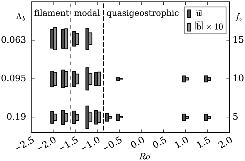
Figure 2: Dynamic regimes of simulations of the DTS device. The heights of the dark (light) markers scale linearly with the kinetic (magnetic) fluctuation levels. The fluctuation levels are calculated by integrating the maps, calculated by Eqn. 7, in $r$ and $\theta$. The velocities and magnetic fields are both in nondimensional units ($1/U_{o}$ for velocity, $V_{A}/U_{o}$ for magnetic fields). The $Em$ and $\Lambda$ of the simulations are chosen to match those of the machine at the various outer rotation rates. (See Tab. 1). The rotation frequency for each $\Lambda_{b}$ value is indicated on the right axis. The $Ek$ of the simulations are set to 10^-6.

This paper will proceed as follows. Section I introduces the numerical code used to model the DTS-$\Omega$ device. Section II shows the analysis of the computed velocity and magnetic fields when they are averaged over time and azimuth. Section III considers the full spatio-temporal data of the simulations and applies several techniques for analyzing them. The persistent modes are subject to a principal component analysis (PCA). The filaments are identified with their magnetic signatures at the surface. Section IV examines the linear stability of the mean velocity and magnetic fields. Section V is a discussion of magnetic measurements at a single meridian on the outer surface of the sphere. This is the measurement that is available on the physical DTS-$\Omega$ device. Section VI are conclusions for this work and perspectives for the future.

I Numerical Model

The dynamical system of the DTS-$\Omega$ is described by the magnetic induction and Navier-Stokes equations for an incompressible fluid. Equations are nondimensionalized by taking as length-scale the radius of the outer sphere $r_{o}$ and as characteristic time $\tau\equiv|\Delta\Omega|^{-1}$ – where $\Delta\Omega\equiv 2\pi(f_{i}-f_{o})$ is the angular velocity difference between the inner and outer sphere. Without loss of generality, $\Delta\Omega>0$, while $\Omega\equiv 2\pi f_{o}$ can be either positive (corotation) or negative (counter-rotation). After choosing characteristic velocity $U_{o}\equiv r_{o}|\Delta\Omega|$, the nondimensionalized magnetic induction equation reads:

$$\partial_{t}\mathbf{b}=\nabla\times\left(\mathbf{u}\times\mathbf{b}\right)+\frac{Em}{|Ro|}\Delta\mathbf{b},$$ (1)

where $\mathbf{u}$ is the incompressible velocity field, $\mathbf{b}$ is the magnetic field, $Ro$ is the (signed) Rossby number $\left(\Omega^{-1}\Delta\Omega\right)$, and $Em$ is the magnetic Ekman number $\left(\eta/r_{o}^{2}\left|\Omega\right|\right.$, with $\eta$ the magnetic diffusivity). The Navier-Stokes equation, in the frame rotating with the outer sphere, is nondimensionalized as

$$\partial_{t}\mathbf{u}+\frac{2}{Ro}\mathbf{\hat{z}}\times\mathbf{u} +\left(\nabla\times\mathbf{u}\right)\times\mathbf{u}=$$ (2)

$$\nabla p^{*} +\frac{Ek}{|Ro|}\Delta\mathbf{u}+\frac{\Lambda_{o}Em}{Ro^{2}}\left(\nabla\times\mathbf{b}\right)\times\mathbf{b}$$

where $Ek$ is the Ekman number $\left(\nu/r_{o}^{2}\left|\Omega\right|\right.$ with $\nu$ the viscosity), $\Lambda_{o}$ is the Elsasser number at the outer sphere $\left(B_{o}^{2}/\mu_{0}\rho\eta\left|\Omega\right|\right.$, with $B_{o}$ the intensity of the imposed magnetic field at $r_{o}$ on the equator, $\mu_{0}$ the magnetic constant, and $\rho$ the density of the liquid), and $p^{*}$ a reduced pressure absorbing all potential forces. The magnetic field is represented in the code as an Alfvén velocity $\left(V_{A}=B/\sqrt{\mu_{0}\rho}\right)$, and the nondimensional magnetic field is thus $V_{A}/U_{0}$. The values of these parameters in the DTS-$\Omega$ are given in Tab. 1. Because $\Lambda_{i}$ is always $>>1$ and $\Lambda_{o}$ is always $<<1$, $\Lambda_{b}$ (the Elsasser number at $r=(r_{i}+r_{o})/2$) is used to give the best intuition as to the importance of the magnetic field in a given simulation. The simulations presented here were designed to match the $Ro$, $Em$, and $\Lambda_{b,o}$ values of the machine as closely as possible. The $Ek$ is treated as a nuisance parameter and set to 10^-6; how and why we treat it that way is handled below.

	$Ek$	$Em$	$Ro$	$\Lambda_{o}$	$\Lambda_{b}$
$f_{o}$	$\frac{\nu}{r_{o}^{2}\left|\Omega\right|}$	$\frac{\eta}{r_{o}^{2}\left|\Omega\right|}$	$\frac{\Delta\Omega}{\Omega}$	$\frac{B^{2}(r=r_{o})}{\mu_{0}\rho\eta\left|\Omega\right|}$	$\frac{B^{2}(r=(r_{i}+r_{o})/2)}{\mu_{0}\rho\eta\left|\Omega\right|}$
5 Hz	4.69$\times 10^{-7}$	6.38$\times 10^{-2}$	[-7.0, 5.0]	1.77$\times 10^{-2}$	0.187
10 Hz	2.35$\times 10^{-7}$	3.19$\times 10^{-2}$	[-4.0, 2.0]	8.87$\times 10^{-3}$	0.095
15 Hz	1.56$\times 10^{-7}$	2.13$\times 10^{-2}$	[-3.0, 1.0]	5.92$\times 10^{-3}$	0.063
20 Hz	1.17$\times 10^{-7}$	1.60$\times 10^{-2}$	[-2.5, 0.5]	4.44$\times 10^{-3}$	0.047

Table 1: Definitions of useful nondimensional parameters for DTS-$\Omega$, and their values/ranges at various outer sphere rotation rates. The two values given for $Ro$ are, respectively, the maximum and minimum values attainable for a given $f_{o}$. The values given for $\Lambda_{o}$ and $\Lambda_{b}$ are, respectively, the Elsasser number at the outer sphere, where the applied field is weakest, and at the middle radius sphere, where the dynamics actually live.

The two dynamical equations are completed by boundary conditions. The no-slip boundary condition applies to the velocity field, namely $\mathbf{u}(r=r_{i})=r\sin\theta\mathbf{\hat{\phi}}$ and $\mathbf{u}(r=r_{o})=0$. The magnetic field matches with potential fields outside the solid shells and the conductivity jumps at the solid-liquid boundaries are treated within the finite difference framework Cabanes.PRE.2014 ; SHTNS . Everything stays spherically symmetric to fit in a spectral framework. However, as the goal is to investigate the properties of a real experiment, the applied magnetic field is chosen to approximate the field of DTS-$\Omega$’s inner magnet, rather than a pure dipole, including magnetic harmonics up to degree 11 and order 6 Cabanes.PRE.2014 . The inhomogeneous magnetic field is rotated in phase with the inner sphere.

Because both velocity $\left(\mathbf{u}\right)$ and magnetic $\left(\mathbf{b}\right)$ fields are divergence free, our three-dimensional spherical code xshells represents them as solenoidal vector spherical harmonics

$$\mathbf{u}(r_{i},\theta,\phi)=\sum\limits_{\ell=\left|m\right|}^{\ell_{max}} \sum\limits_{m=-m_{max}}^{m_{max}}\nabla\times\nabla\times s_{\ell,m}(r_{k})Y_{\ell}^{m}(\theta,\phi)\mathbf{\hat{r}}$$

$$+\nabla\times t_{\ell,m}(r_{k})Y_{\ell}^{m}(\theta,\phi)\mathbf{\hat{r}}\quad\qquad{\rm and}$$

$$\mathbf{b}(r_{k},\theta,\phi)=\sum\limits_{\ell=\left|m\right|}^{\ell_{max}} \sum\limits_{m=-m_{max}}^{m_{max}}\nabla\times\nabla\times S_{\ell,m}(r_{k})Y_{\ell}^{m}(\theta,\phi)\mathbf{\hat{r}}$$

$$+\nabla\times T_{\ell,m}(r_{k})Y_{\ell}^{m}(\theta,\phi)\mathbf{\hat{r}},$$ (3)

where $Y_{\ell}^{m}$ are scalar spherical harmonics. The radial functions are evaluated at every radial grid point, and their derivatives are taken by second order finite difference. The forwards and backwards spherical harmonic transforms are carried out using the efficient SHTns library SHTNS . xshells performs the time stepping of Eqn. 2 in the fluid spherical shell, and the time stepping of Eqn. 1 in both the conducting walls and the fluid. It uses a semi-implicit Crank-Nicholson scheme for the diffusive terms, while all other terms are handled by an Adams-Bashforth scheme (second-order in time). The time, space, and spectral resolutions of the simulations vary most strongly with $Ek$ for numerical stability. The resolutions for the runs presented here are specified in appendix B.

Preliminary simulations in the range $10^{-5}>Ek\geq 10^{-7}$ suggested that $Ek$ serves to set the spatial resolution required for numerical stability, but does not drastically affect the dynamics of the large eddies in the bulk flow, as long as $Ek$ is small enough. The induced magnetic spectra were similarly agnostic to $Ek$. Thus we make two assumptions in the interest of reducing the necessary spectral resolution. The first is that $Ek=10^{-6}$ adequately represents the large scale component of the flow. The second is that a hyperviscosity Glatzmaier.PEPI.1995 adequately models the turbulent cascade to small scales in the Ekman layer. To justify this, Fig. 3 shows the energy in each azimuthal harmonic $m$ as a function of radius. The higher order harmonics are only really visible in the outermost 0.005 of the sphere. The underlying assumption of hyperviscosity is that, for a turbulent cascade, there is a net transfer of energy to smaller and smaller scales through a Kolmogorov cascade, and that this energy transfer can be modeled as an effective viscosity that increases in value at smaller and smaller scales. Our simulations use a modified version of the hyperviscosity Nataf2015 , that only applies to the angular part of the Laplace operator and to the last 20 $\left(\ell_{0}>0.8\ell_{max}\right)$ according to

$$\nu_{\ell>\ell_{0}}=\nu_{0}\times h^{\left(\ell-\ell_{0}\right)/\left(\ell_{max}-\ell_{0}\right)}$$ (4)

where $\nu_{0}$ is the base viscosity and $h$ is the ratio between the viscosity at $\ell_{max}$ and $\nu_{0}$, here chosen to be 1000.

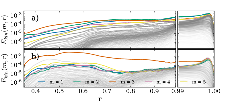
Figure 3: Colormaps showing kinetic energy in each $m>0$ azimuthal wavenumber as a function of spherical radius for (a) $Ro=-2.0,\Lambda_{b}=0.095$ and (b) $Ro=-1.0,\Lambda_{b}=0.095$. The $m\in[1,5]$ are colored, the others have their opacity set as a function of the largest value in the bulk flow. A zoom of the last 0.01 is shown on the right.

In the majority of cases at $\Lambda_{b}=0.19,0.095$, the simulations were initialized from a previous set of simulations with identical $Ro$ and slightly different $\Lambda$ and ${\rm E_{m}}$. The simulations at $\Lambda_{b}=0.063$ were initialized from runs at the same $Ro$ at $\Lambda_{b}=0.095$. The runs at $Ro=-0.50,-0.75$, and $-1.75$ were seeded off simulations at $Ro=-1.00,-0.50$, and $-1.50$ respectively. In all cases, the analyses are carried out after waiting 40 differential rotation periods for the new simulation to settle. Unless otherwise mentioned, statistics and analyses are reckoned over 60 differential rotation periods.

II Time averaged spatial data

The diagram of Fig. 2 shows the kinetic and magnetic fluctuation levels of the simulations. These fluctuations are defined in a frame of reference rotating with the inner sphere

$$\overline{\mathbf{b}}(r,\theta,\phi) =\frac{1}{N}\sum\limits_{i=1}^{N}\mathbf{b}(r,\theta,\phi,t_{i}){\rm,\;and}$$ (5)

$$\widetilde{\mathbf{b}}(r,\theta,\phi,t_{i}) =\mathbf{b}(r,\theta,\phi,t_{i})-\overline{\mathbf{b}}(r,\theta,\phi).$$ (6)

The corotation is necessary for the magnetic fluctuations because the applied field is three dimensional. A two dimensional map of the kinetic or magnetic energy densities can be found by integrating

$$\left\langle\widetilde{\mathbf{b}}\cdot\widetilde{\mathbf{b}}\right\rangle(r,\theta)=\frac{1}{N}\sum\limits_{i=1}^{N}\frac{1}{2\pi}\int\limits_{0}^{2\pi}d\phi\widetilde{\mathbf{b}}\cdot\widetilde{\mathbf{b}}(r,\theta,\phi,t_{i}).$$ (7)

these maps, when integrated in $r$ and $\theta$, give the values represented in Fig. 2.

The maps of kinetic and magnetic fluctuation levels for several flows are shown in Fig. 4. The top row shows the kinetic fluctuation levels with isocontours of the angular velocity overplotted; the dashed lines indicate the region of superrotation (i.e., where the fluid rotates with an angular velocity larger than that of the inner sphere Brito.PRE.2011 ). The bottom row shows the magnetic fluctuation levels with fieldlines of the poloidal magnetic field overplotted. Maps for $Ro=1.5,-1.0,$ and $-2.0$, all at $\Lambda_{b}=0.095$, are shown in successive columns. These flows were chosen as exemplar of the various different dynamic regimes. The flow at $Ro=1.5$ is defined by low fluctuation levels of both the kinetic and magnetic fields. The mean flow is decidedly quasigeostrophic, with only the barest nub of a superrotary region near the equator of the inner sphere. The $Ro=-1.0$ flow has a quasigeostrophic region near the outer edge, but the dominant feature of both the mean flow and the fluctuations is a large superrotary region extending into bulk flow where the strongest of the kinetic and magnetic fluctuations live. The $Ro=-2.0$ flow starts to return to quasigeostrophy, although the bulk flow has not quite reached a state of z invariance. Here the fluctuations of the kinetic energy live predominantly towards the outer sphere, while the strongest magnetic fluctuations are concentrated more towards the inner sphere. This is not particularly surprising, as the applied magnetic field is 27 times stronger at the inner sphere than the outer.

In section III we will see that the fluctuations at $Ro=-1.0$ are characterized by persistent structures with a fairly well defined spatial location, while the fluctuations at $Ro=-2.0$ are characterized by intermittently formed structures that propagate poleward from their point of origin. This means that the time averages of Fig. 4b give a good indication of the shape of the fluctuations being averaged over, while the time averages of Fig. 4c smear the structures out over the region they propagate through. As the fluctuations in the case of positive differential rotation were significantly smaller in scale and in amplitude than those for negative differential rotation, they will be ignored in the following discussion.

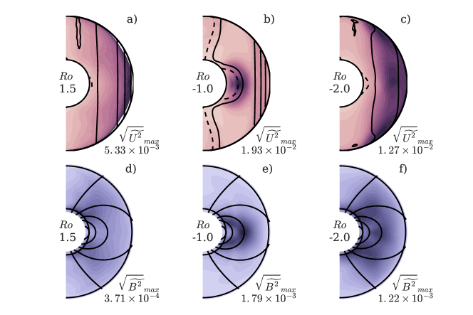
Figure 4: Colormaps showing fluctuation levels of the magnetic and velocity fields. The first row, (a, b, and c), shows the kinetic fluctuations, the second row, (d, e, and f), shows the magnetic fluctuations. The numbers on the lower right indicate the maximum value of the energy density (excluding the Ekman layer). The contour lines in the first row represent isocontours of angular momentum of the bulk fluid. Inside the dashed line the bulk fluid is rotating faster than the inner sphere in the reference frame of the outer sphere. The contour lines in the second row are field lines of the mean poloidal magnetic field. Each column presents a set of parameters firmly in the quasigeostrophic (a and d), modal (b and e), and filamentary (c and f) regimes. All of the fluctuation levels are calculated for $\Lambda_{b}=0.095$.

III Spatio-temporal analysis

III.1 Modal flows

The flows at $Ro=-1.2,-1.0$ revealed fluctuations living deep in the bulk of the flow. Figure 5 shows the time and azimuthally averaged kinetic and magnetic fluctuations at $Ro=-1.2,\Lambda_{b}=0.095$ (a and c respectively) and for $Ro=-1.0,\Lambda_{b}=0.095$ (b and d). The streamlines of the mean meridional flow are plotted over each map. Both cases include an outward streaming jet originating at the equator of the inner sphere and an inward streaming jet originating at the equator of the outer sphere. The difference is that at $Ro=-1.2$ the outward jet dominates the mean flow, extending to a radius of 0.82, while at $Ro=-1.0$ the inward jet dominates from a radius of 0.40. In both cases the oppositely directed jet is too weak to be seen in the streamlines.

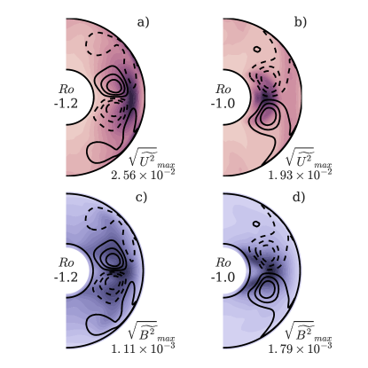
Figure 5: As in Fig. 4, but only for modal flows. The contour lines represent streamlines of poloidal circulation. Solid lines are counter-clockwise circulation; dashed lines are clockwise circulation. All of the energies are calculated for $\Lambda_{b}=0.095$.

The kinetic fluctuations at $Ro=-1.2$ live predominantly near the stagnation point, $\left(u_{s}=0\right)$; those at $Ro=-1.0$ live in the jet itself $\left(\left|u_{s}\right|_{max}\right)$ as shown in Fig. 6. The jets velocities are shown in Fig. 6a. The azimuthal flows, shown in Fig. 6b, and background magnetic fields, shown in Fig. 6c, do not seem to determine whether a location is stable or not, but their profiles are noted for a later use.

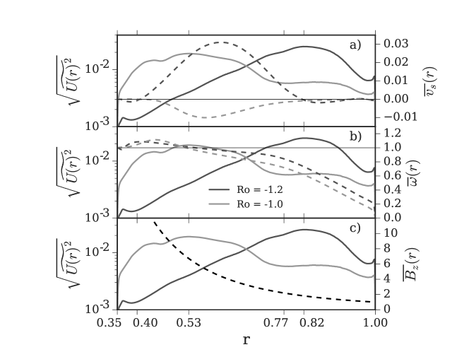
Figure 6: Kinetic fluctuation levels at the equator (solid lines) for Ro = -1.2 and Ro = -1.0 and $\Lambda_{b}=0.095$ in log-scale (on the left) as a function of $r$. The (a) bulk flows’ cylindrically radial velocity, (b) bulk flows’ angular velocities, and (c) imposed vertical magnetic field in the equatorial plane are plotted as dashed lines with the vertical scales on the right. The radii of the peak fluctuation levels are noted on the x-axis.

These fluctuations proved susceptible to a principle component analysis (PCA, see Appendix C), where a spatio-temporal signal is decomposed into individual spatial structures that evolve independently of each other in time. The first three of these structures for $Ro=-1.0,\Lambda_{b}=0.095$, averaged in azimuth and split into equatorially antisymmetric components in the ’northern’ hemisphere and equatorially symmetric components in the ’southern’ hemisphere, are shown in Fig. 7 (a-c) with their time series shown in Fig. 7d. The streamlines of the meridional flow are plotted over the maps. All three modes are very clearly symmetric about the equator, and the first mode very clearly dominates the others over the time period analyzed. The same decomposition is shown for $Ro=-1.2,\Lambda_{b}=0.095$ in Fig. 8. The dominant mode (a) is antisymmetric about the equator, but it arises in chaotic bursts for these parameters. (This mode is more clearly dominant at $\Lambda_{b}=0.19$, see Fig. 16 in Appendix A).

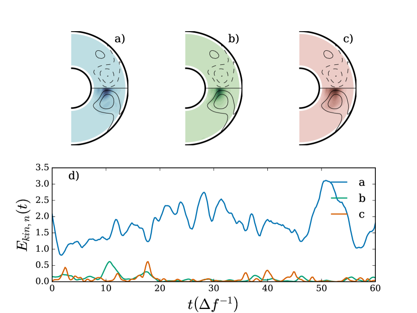
Figure 7: (a-c) Colormaps showing azimuthally averaged kinetic energy density of the first three singular modes of the $Ro=-1.0,\Lambda_{b}=0.095$ flow. The upper hemisphere shows the equatorially antisymmetric component of the mode; the lower hemisphere shows the equatorially symmetric component. (d) The energy in each mode (a-c) as a function of time, scaled against the mean energy in the kinetic fluctuations of the raw signal. Only the region $r\in[0.425,0.975]$ is included in the PCA.

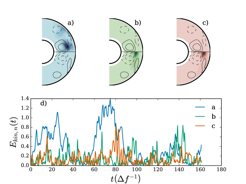
Figure 8: (a-c) Colormaps showing azimuthally averaged kinetic energy density of the first three singular modes of the $Ro=-1.2,\Lambda_{b}=0.095$ flow. The upper hemisphere shows the equatorially antisymmetric component of the mode; the lower hemisphere shows the equatorially symmetric component. (d) The energy in each mode (a-c) as a function of time, scaled against the mean energy in the kinetic fluctuations of the raw signal. Only the region $r\in[0.425,0.975]$ is included in the PCA.

Figure 9 shows 3-d renderings of the dominant principal component, both the velocity field (a,b) and the surface magnetic field associated with it (c,d) for $Ro=-1.2$ (a,c) and $Ro=-1.0$ (b,d). The dominant mode is antisymmetric at $Ro=-1.2$ and has a predominant azimuthal mode number $m=2$, while it is symmetric at $Ro=-1.0$ with $m=3$. It is worth noting that the background magnetic field, shown in Fig. 6(c) is $3.5\times$ larger at the $Ro=-1.0$ fluctuation peak than at the $Ro=-1.2$ peak.

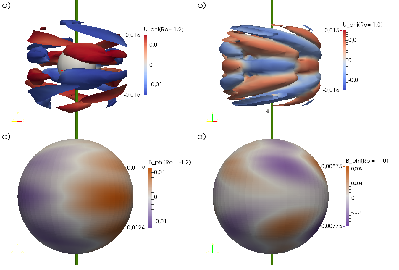
Figure 9: Paraview rendering of the velocity component (a) and the surface magnetic field (c) of the first principle component at $Ro=-1.2,\Lambda_{b}=0.095$. Figures b) and d) are the same for $Ro=-1.0,\Lambda_{b}=0.095$. The surfaces in a) and b) are isocontours of $\left|\mathbf{u}\right|$, at $0.15U_{0}$ and $0.10U_{0}$ respectively, with the azimuthal velocity painted on the surface. The azimuthal magnetic field of the components (scaled against $B_{o}$). at the surface of the outer sphere are shown in c) and d). The inner sphere is visible in (a); the green cylinders represent the rotation axis.

This behavior connects the modes seen here with those found in other simulations of MSC flow. For MSC flow without global rotation and a vertical, homogeneous applied field, Hollerbach Hollerbach.RSPA.2009 found equatorially antisymmetric instabilities of the equatorial jet at low applied magnetic field and equatorially symmetric instabilities of the stagnation point at an applied field about $2.5\times$ stronger (depending on the rotation of the inner sphere). The magnetic fields in these simulations were comparable to those performed here (equivalent to $10^{-3}<\Lambda<5\times 10^{-2}$, see Appendix B). Continuing on this, Gissinger et al. Gissinger.PRE.2011 explored a similar system with a dipole magnetic field and global rotation (equivalent to $Ro=3.5,\;0.007\leq\Lambda_{o}\leq 2.8$ by our definitions ) and found a similar set of instabilities changing from antisymmetric to symmetric about the equator as the applied magnetic field was increased. The modes found here are novel in that the jet’s instability is equatorially symmetric and the return flow instability is antisymmetric. This suggests that the actual stability of the background flows in all of these cases is agnostic to the magnetic field entirely, but that the symmetry is determined by the strength of the vertical field where the instability arises. It is worth noting that the other principle components of $Ro=-1.2$ resemble the principle component of $Ro=-1.0$ in shape and symmetry.

III.2 Filamentary flow

When the differential rotation is increased beyond $Ro=-1.2$, the fluctuations move out of the bulk flow and take up residence along the outer sphere. Here they form long, thin filaments, at predominantly m=1, that are carried towards the pole by the meridional circulation. At these higher latitudes, they split up along the azimuthal coordinate. Figure 10 shows (a) a 3-d rendering of an isocontour of kinetic energy and (c) the latitudinal magnetic field at the surface and the magnetic field lines originating on the kinetic isocontours and extending out of the sphere. The same is shown at a time 16 differential rotation periods later, as the filament is breaking up, in (b & d), though the surface field is azimuthal in (d). The magnetic field lines extending from the kinetic structures into the vacuum are also shown in (c & d). These snapshots were taken from a simulation at $Ro=-2.0$ and $\Lambda_{b}=0.095$

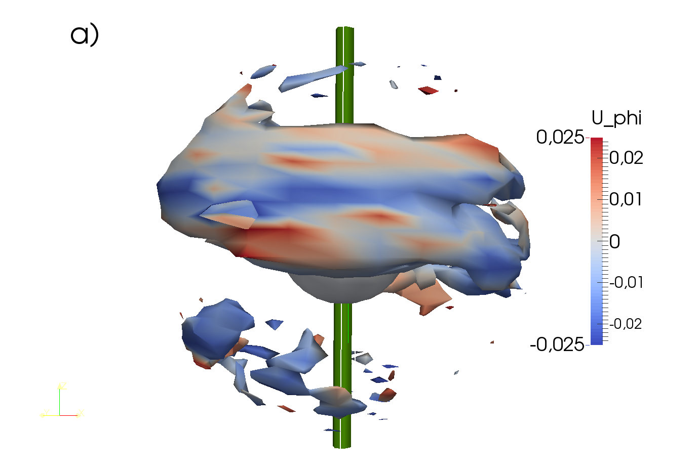
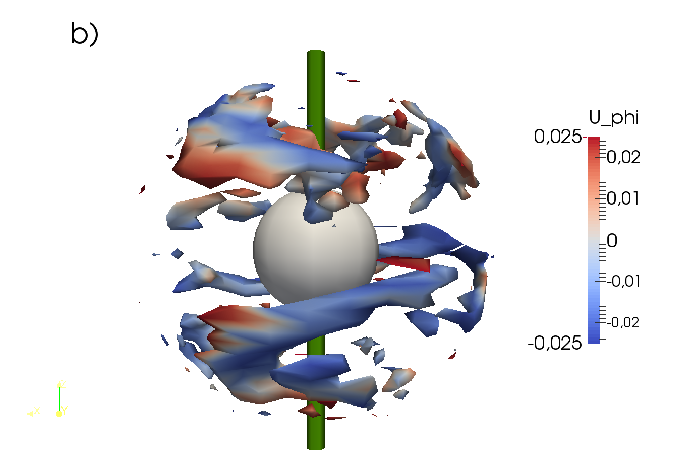
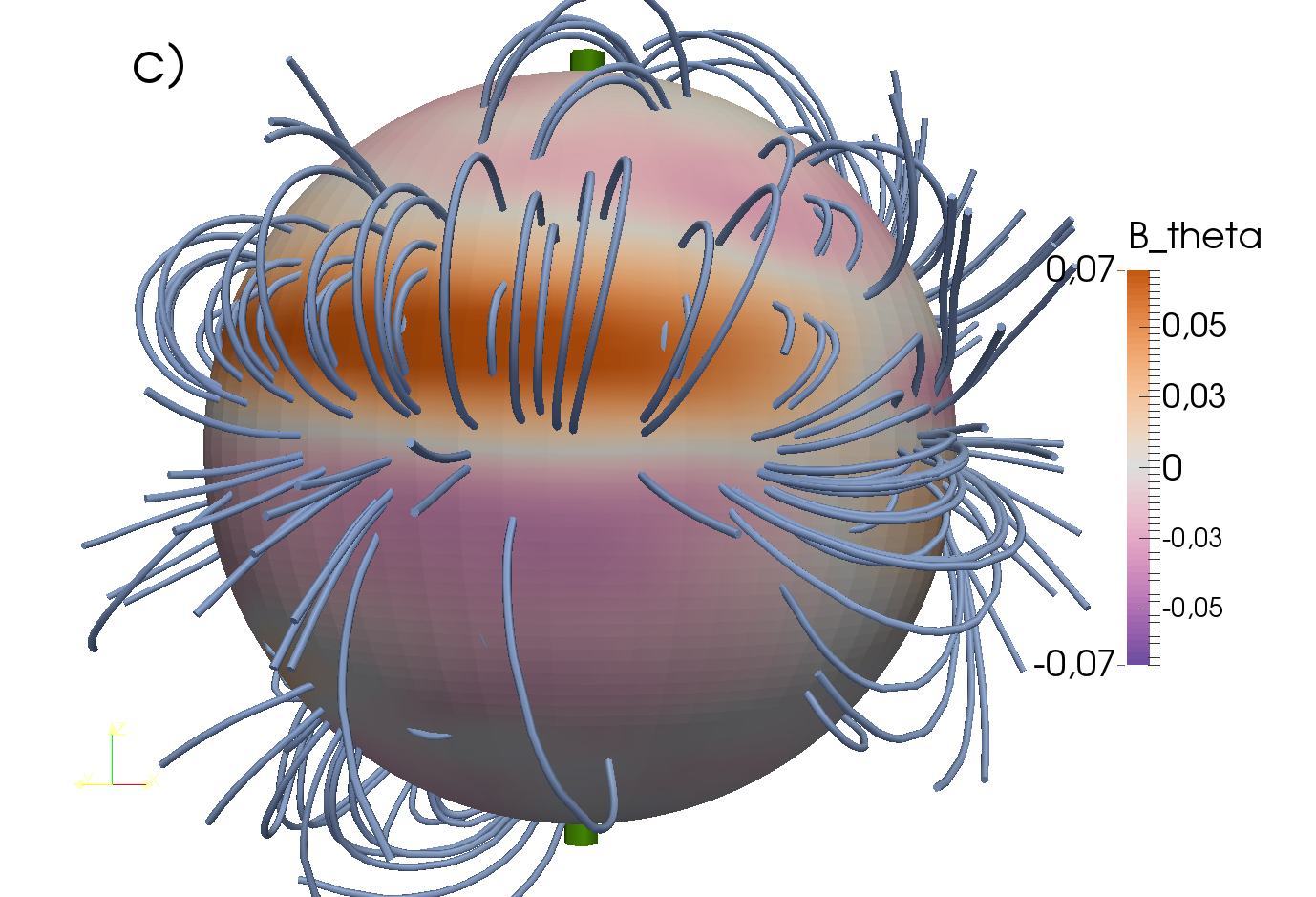
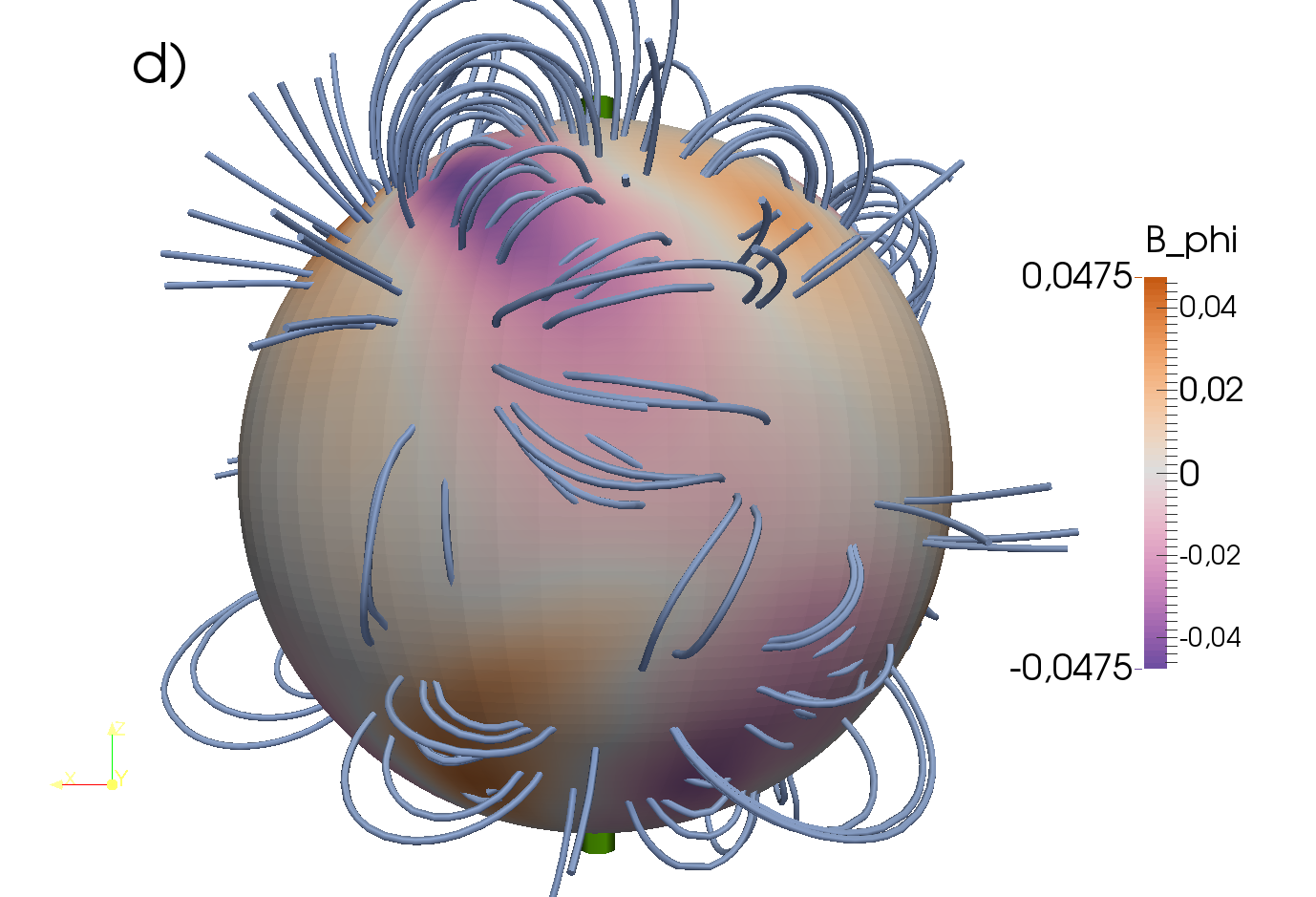
Figure 10: Paraview PARAVIEW rendering of two individual snapshots of the flow at $Ro=-2.0$ and $\Lambda_{b}=0.095$. The renderings show (a) an isosurface of $\left|\widetilde{\mathbf{v}}\right|$ corresponding to 0.025 $U_{0}$ and (b) the same contour $16\Delta f^{-1}$ later. The isosurfaces are painted with the azimuthal velocity. The surface magnetic fields, scaled against $B_{o}$ of these snapshots are shown in (c) and (d) respectively, along with the magnetic field lines originating at the isocontours. The latitudinal field is shown for (c), the azimuthal field for (d). The green cylinders represent the rotation axis.

The surface magnetic field seems to be a good indicator of the flow underneath. Figure 11a shows the cylindrically integrated kinetic energy,

$$E_{kin}(z,t)=\int\limits_{0}^{2\pi}d\phi\int\limits_{0}^{\sqrt{1-z^{2}}}ds\;\mathbf{\widetilde{u}\cdot\widetilde{u}}(s,z,\phi,t),$$ (8)

where $s$ is the cylindrical radius $s=r\sin\theta$ and $z$ is the cylindrical height $z=r\cos\theta$. The latitudinal field at the surface, averaged in $\phi$ is shown in Fig. 11b. The times Fig. 10 are taken from are indicated. The latitudinal field component corresponds well with the kinetic fluctuations near the equator (below $\sim 40^{\circ}$). The azimuthal field (not shown) has a stronger correspondence towards the poles. As seen in Fig. 10, the kinetic fluctuations are elongated more in $\phi$ towards the equator and more in $\theta$ towards the pole; the induced magnetic field seems strongest in the direction perpendicular to the elongation. This will be shown more in Section V.

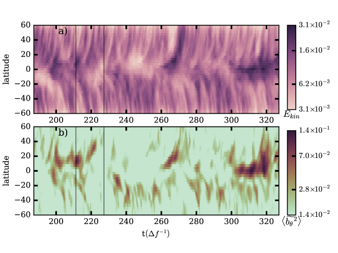
Figure 11: a) Cylindrically Integrated kinetic energy vs latitude and time. b) Azimuthally integrated $\widetilde{b_{\theta}}^{2}$ at the surface (scaled against $\left.B_{o}\right)$ vs latitude. Filamentary regime at $Ro=-2.0$ and $\Lambda_{b}=0.095$. The vertical lines indicate the snapshots the renderings of Fig. 10 are taken from.

Previous simulations of the experiment with a stationary outer sphere also turned up two classes of fluctuations: a centripetal jet instability near the equator, and a Bödewalt type instability originating in the upper latitudes (above $\sim$40^∘) both propagating poleward Figueroa.JFM.2013 . The Bödewalt type instability is likely not present here, as the angular velocity profile at the outer sphere’s pole (Figueroa.JFM.2013 Fig. 3) is replaced by an Ekman type boundary layer when the outer sphere rotates. The centripetal jet instabilities demonstrated some similar behavior to the filaments seen here. Specifically, structures generated near the outer sphere’s equator are swept poleward by the meridional flow.

IV Linear instabilities of the mean fields

What is the origin of the modes observed in the various regimes? We use the time- and phi-averaged fields from the non-linear simulations as base flow $\bar{\mathbf{U}}$ and magnetic field $\bar{\mathbf{B}}$ for linear stability tests. Note that for these base fields, we keep only the dominant symmetry: $\bar{\mathbf{U}}$ is symmetric while $\bar{\mathbf{B}}$ is anti-symmetric with respect to the equatorial plane. We time-step the linearized MHD equations for the velocity and magnetic field perturbations $\mathbf{u}$ and $\mathbf{b}$ using the linearized xshells code vidal2018 , waiting for the growth-rate to stabilize. We distinguish hydrodynamic stability ($\bar{\mathbf{B}}=0$, hence no Lorentz force), purely magnetic stability ($\bar{\mathbf{U}}=0$, but $\nabla\times\bar{\mathbf{B}}\neq 0$) from magnetohydrodynamic (MHD) stability (using both $\bar{\mathbf{B}}$ and $\bar{\mathbf{U}}$). By comparing these three cases, we can determine if the MHD instability is merely a hydrodynamic instability, or if the magnetic field plays a more fundamental role. Results are summarized in table 2. First, the mean magnetic configurations alone ($\bar{\mathbf{U}}=0$) are found always stable at the field strengths of this study. Then, we find that the growth rate of the MHD perturbation is always smaller than the hydrodynamic one. These two observations suggest that the mean magnetic field and associated electric current have no driving effect but rather a damping effect on instabilities driven by the mean velocity field.

Looking at individual cases, we see that for $Ro=-2.0$, the mean flow is subject to a strong hydrodynamic instability of the outer boundary layer, where the magnetic field is weaker. This happens for the two base flows obtained with different field strength (as measured by $\Lambda_{b}$). For $Ro=-1.0$ and $Ro=-1.2$, the intensity of the perturbations have been reported in figure 12. For $Ro=-1.2$, depending on the field strength $\Lambda_{b}$, the mean flow may be subject to a similar hydrodynamic instability of the outer boundary layer (but for a lower wavenumber) or to an instability localized at the equator of the inner-sphere (Fig. 12d). In both cases, this hydrodynamic instability does not survive the additional damping due to the magnetic field, which favors a bulk instability of low wave number ($m=4$, Fig. 12e,f). For $Ro=-1.0$, both hydrodynamic and MHD instabilities occur away from the boundary layers. They are similar, but the MHD instability seems to be slightly pushed away from the strong field inner-core to a region were the magnetic field is lower (compare Fig. 12a and b). Note that for all cases investigated, the MHD perturbations show little dependence upon $\Lambda_{b}$.

		hydrodynamic instability			MHD instability
$Ro$	$\Lambda_{b}$	$m$	$\sigma$	localization	$m$	$\sigma$	localization
-2.00	0.190	22	1.59	outer boundary layer	22	1.55	outer boundary layer
	0.095	22	1.30	outer boundary layer	22	1.29	outer boundary layer
-1.20	0.190	5	0.264	outer boundary	4	0.198	like fig. 12e,f
	0.095	18	0.2961	see fig. 12d	4	0.2235	see fig. 12e,f
-1.00	0.190	3	0.1931	like fig. 12a	2	0.0483	like fig. 12b,c
	0.095	3	0.1828	see fig. 12a	2	0.0569	see fig. 12b,c

Table 2: Instability of the mean flow of several runs (see table 3 for the corresponding non-linear runs). $m$ is the unstable azimuthal wave number, $\sigma$ is the non-dimensional growth rate, and ‘localization’ indicates the localization of the instability in the meridional plane.

Figure 12: Colormaps of the intensity of the most unstable mode (white is zero). Top row (a,b,c): $Ro=-1.00$ and $\Lambda_{b}=0.095$. Bottom row (d,e,f): $Ro=-1.20$ and $\Lambda_{b}=0.095$. Left (a,d) shows the hydrodynamic instability while middle (b,e) and right (c,f) represent respectively the velocity and magnetic intensity of the magnetohydrodynamic instability. The contours in (a,b,d,e) are iso-lines of the angular velocity of the mean flow $\bar{\mathbf{U}}_{\phi}/s$ with magenta for super-rotation. The contours in (c,f) are iso-lines of the the toroidal mean magnetic field $\bar{\mathbf{B}}_{\phi}$ (dashed for negative). All velocity eigenmodes are equatorially symmetric while the magnetic ones are anti-symmetric.

We can now compare these instabilities with the fully nonlinear simulations. First, at $Ro=-1.0$ and $\Lambda_{b}=0.095$ the PCA analysis shows a mode dominated by an $m=3$ symmetry (Fig. 7 and 9b), while the most linearly-unstable mode has $m=2$. The detailed structure differ (not shown), but the same equatorial symmetry is recovered.

We now turn to $Ro=-1.2$ and $\Lambda_{b}=0.095$ for which the PCA analysis shows a mode dominated by $m=2$ and anti-symmetric with respect to the equator (Fig. 8 and 9a). Instead, the linearly-unstable mode has $m=4$ and is symmetric (not shown). Comparing figure 8 with figure 12e, we see that the most unstable MHD mode resembles the second and third PCA (labeled b and c respectively) but not the first one which has opposite symmetry. The PCA analysis thus suggests an interplay between two MHD instabilities, the most unstable (symmetric) and probably the second most unstable (anti-symmetric).

Finally, for $Ro=-2$, the most unstable mode is located at the outer boundary (not shown) and we expect it to continuously generate turbulent flow that fills the bulk and leads to the filamentary regime.

All these observations support that instabilities are triggered by the mean flow, while the applied magnetic field selects, damps and reshapes them, keeping in mind that the mean flow itself is strongly affected by the presence of the applied magnetic field. Interestingly, large-scale coherent structures emerging from hydrodynamical turbulence have also been linked to linear stability of their base flow herbert2014 ; brethouwer2014 , while exhibiting bursts as seen in figure 8. It is thus likely that in our system, linear instabilities growing on the mean flow lead to the persistent or intermittent structures observed in the various turbulent flow regimes described here.

V Simulated Probes

The trade-off between experimental and numerical physics is that it is easy to get time series of experimental data, but difficult to extend that data outside a small domain that is amenable to direct measurement, while it is easy to see all of the structures within a simulation at the cost of large amounts of computing time. The longest simulations presented here correspond to 10-20 s of runtime on DTS-$\Omega$. Given the full spatial data included in the simulation outputs, it is easy to produce simulated probes and associate these signals to specific structures. In this section we calculate the magnetic field at the outer surface on a single meridian over from snapshots taken at a rate of 50 per differential rotation period. All reported values for magnetic measurements are scaled against the intensity of the magnetic field at the outer sphere’s equator $B_{o}$ for ease of comparison between the simulations and the experiment (where $B_{o}$ is 7.4 mT). All of these simulations were carried out at $\Lambda_{b}=0.095$, equivalent to an outer sphere rotation frequency of 10 Hz. The results can directly be compared to the experimental examples of figure 1.

V.1 Modal Flows

The kinetic structures of Fig. 9 have specific azimuthal orders (m) and equatorial symmetries and are rotating relative to the outer sphere. Thus the magnetic field at the surface of the sphere should behave entirely as a function of the shape and rotation of the underlying structure. Figure 13 shows the magnetic field at the surface for (a) Ro = -1.2 and (b) Ro = -1.0, as well as the measurable field associated with the dominant principle component for each (c and d respectively). As in Fig. 9, the magnetic structures at Ro = -1.2 are vertical, and sweep past the probe with a frequency of $1.7\Delta f$ (rather, an m=2 structure rotating with a frequency of $0.85\Delta f$). The magnetic structures at Ro = -1.0 are helical and sweep past the probe with a frequency of $2.9\Delta f$ (rather an m=3 structure rotating at $0.96\Delta f$). In both cases, the full signal strongly resembles that of the dominant mode with additional signals on top. This is not preordained, as the PCA was computed over the entire volumetric dataset, and emphasizes again that the surface measurements are strongly connected to the global dynamics. The rotation rates are related to the mean flow of the background at the location of the structure; Fig. 6 indicates the locations where the bulk flow in the equator rotates at the rate of the structure ($r=0.53$ for $Ro=-1.0$, and $r=0.77$ for $Ro=-1.2$).

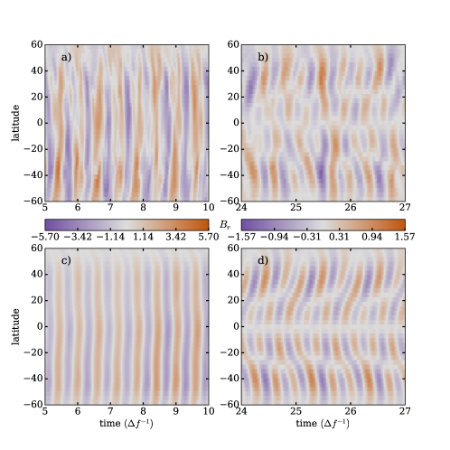
Figure 13: Radial component of the surface magnetic field (as a percentage of $B_{o}$ at a single meridian on the outer sphere vs time at a) Ro = -1.2 and b) Ro = -1.0 at $\Lambda_{b}=0.095$. The signal from the dominant principle component is shown below in c) and d) respectively.

V.2 Filamentary Flows

The filaments of Section III.2 have broader azimuthal extent than the modes of the previous discussion. They are not easily divided into single azimuthal modes numbers, but the volume renderings of Fig. 10 show an apparent combination of m=1 and m=2, depending on the latitude. The latitudinal and azimuthal surface fields of Fig. 14 a & b (respectively), and their spectra in Fig. 14c & d provided some corroboration. The latitudinal field has the strongest spectral energy near the equator at a frequency of 0.75$\Delta f$, and noticeable peaks near 1.5 and 2.25 $\Delta f$ (that is 2 or 3 times the fundamental) at higher latitudes. The azimuthal field at the surface is much stronger at higher latitudes and at the higher frequencies. Note also the low frequency modulation at frequency $\simeq 0.1\Delta f$, visible on the $B_{\theta}$ probes and their spectra, especially around the equator and 20 to 30^∘ degrees of latitude, most certainly related to the poleward sweeping of the filaments (see III.2).

Figure 14: The surface magnetic field, as a percentage of $B_{o}$ at a single meridian on the outer sphere vs time at $Ro$ = -2.0 and $\Lambda_{b}=0.095$, broken up into (a) latitudinal and (b) longitudinal components. The second row (c & d respectively) shows the power spectral density of the magnetic signal at each latitude on that meridian. The color scale is truncated at one half the maximum spectral level to help highlight the higher harmonics.

VI Conclusions

We have carried out a set of magnetized spherical Couette (MSC) flow simulations at nondimensional parameters relevant to the DTS-$\Omega$ machine. These simulations have found a set of different dynamic regimes. For positive (and weakly negative, $Ro\geq-0.5$) differential rotation the flows were characterized by low fluctuation levels on top of quasigeostrophic base flows. At stronger, negative differential rotation, the flow consists of large scale internal structures, associated with magnetic signatures at the surface. At moderate, negative differential rotation, $Ro$=-1.0 and -1.2, these structures are persistent, with a specific azimuthal order, rotating with the bulk flow. At stronger differential rotation, $Ro$=-2.0, these structures are intermittent (with lifespan around 10 differential rotation periods), with large azimuthal extent, that propagate poleward from their point of origin.

Given that simulations of MSC flow contain the full structures of the kinetic and magnetic fields, it is easy to draw relations between the one and the other. What is more difficult is taking the surface magnetic fields alone, i.e the diagnostic which is most readily available to the physical DTS-$\Omega$ device, and inferring the structure of the velocity field that induces it. Nevertheless, some broad inferences can be made from the surface fields and their spectra. The shift from persistent structures to intermittent filaments corresponds to a shift from a single dominant frequency in magnetic field measurements to multiple bands depending on latitude and direction of the magnetic field.

The persistent structures have precedence in other simulations of MSCF, including those carried out with no global rotation Hollerbach.RSPA.2009 and those carried out with positive differential rotation Gissinger.PRE.2011 . (That our modes occur at different values of $\left|Ro\right|$ is not so surprising. Positive and negative differential rotation are not the same, but they can demonstrate similar dynamics with offset $\left|Ro\right|$ Zimmerman.JGR.2014 ). In all cases these structures arise from hydrodynamic instabilities of the meridional circulation (either in the equatorial jets or near the stagnation points). What is novel about the structures here is that the equatorial symmetry of these instabilities is reversed from those of Hollerbach.RSPA.2009 ; Gissinger.PRE.2011 . We attribute this to the strength of the background magnetic field. We have shown that, although the magnetic field determines the shape of the mean flow in all cases, these two dimensional flows are stable or unstable to three dimensional hydrodynamic instabilities independent of the magnetic field. The effect of the magnetic field is then to select and reshape the instability. By doing this, an instability with symmetry opposite to the expected hydrodynamic instability can be observed, depending on the magnetic field strength. The symmetric instability at the stagnation point ($Ro=-1.2$) is compatible with an oscillation of that point within the plane of the equator as the strength of the colliding jets oscillate. In contrast, the antisymmetric instability of the inward jet ($Ro=-1.0$) is reminiscent of the instability that deflects the jet up or down DumasThesis ; Hollerbach2006 ; Wicht.JFM.2013 .

The intermittent filaments seen here in the most turbulent cases share some features with the inward jets emerging from the outer sphere and drifting poleward in simulations of the DTS device without outer rotation Figueroa.JFM.2013 . However, the filaments evidenced in this work appear to last significantly longer.

We emphasize that all the coherent structures seen in our simulations appear on top of a fully turbulent state. Such a phenomenon has also been documented in hydrodynamical turbulence herbert2014 ; brethouwer2014 , where the instabilities of the mean flow play an important role too.

Our simulations have also shown that the surface measurements of the magnetic fields are significantly affected by flow dynamics deep in the shell. This means that the many measurements that will be available on the DTS-$\Omega$ machine will likely help to evidence the flow regimes identified here, and beyond.

VII Acknowledgments

The XSHELLS code used for the numerical simulations is freely available at https://bitbucket.org/nschaeff/xshells. We thank two anonymous reviewers for fruitful suggestions. This work was funded by the French Agence Nationale de la Recherche under grant ANR-13-BS06-0010 (TuDy). We acknowledge GENCI for awarding us access to resource Occigen (CINES) under grant x2015047382 and x2016047382. Part of the computations were also performed on the Froggy platform of CIMENT (https://ciment.ujf-grenoble.fr), supported by the Rhône-Alpes region (CPER07_13 CIRA), OSUG@2020 LabEx (ANR10 LABX56) and Equip@Meso (ANR10 EQPX-29-01). ISTerre is part of Labex OSUG@2020 (ANR10 LABX56).

Appendix A Modal flows at $\Lambda_{b}=0.190$

As shown in Fig. 2, simulations were carried out at three values of $\Lambda_{b}$. Those discussed in the main text come primarily from the case where $\Lambda_{b}=0.095$, mostly to make comparison easier between the modal and filamentary flows. The modal structures and dominance of a single mode over the others is much more clear in the case where $\Lambda_{b}=0.190$. The decompositions of $Ro=-1.0,\Lambda_{b}=0.190$ and $Ro=-1.2,\Lambda_{b}=0.190$ are shown in Figs. 15 & 16 respectively. Note that the profiles of the various modes are very similar to those of Figs. 7 & 8. The time series show the primary difference between $\Lambda_{b}=0.190$ and $\Lambda_{b}=0.095$, in Fig. 16, the antisymmetric mode (a) is unambiguously the dominant mode (excepting a few bursts of mode (b) where they reach equal energies).

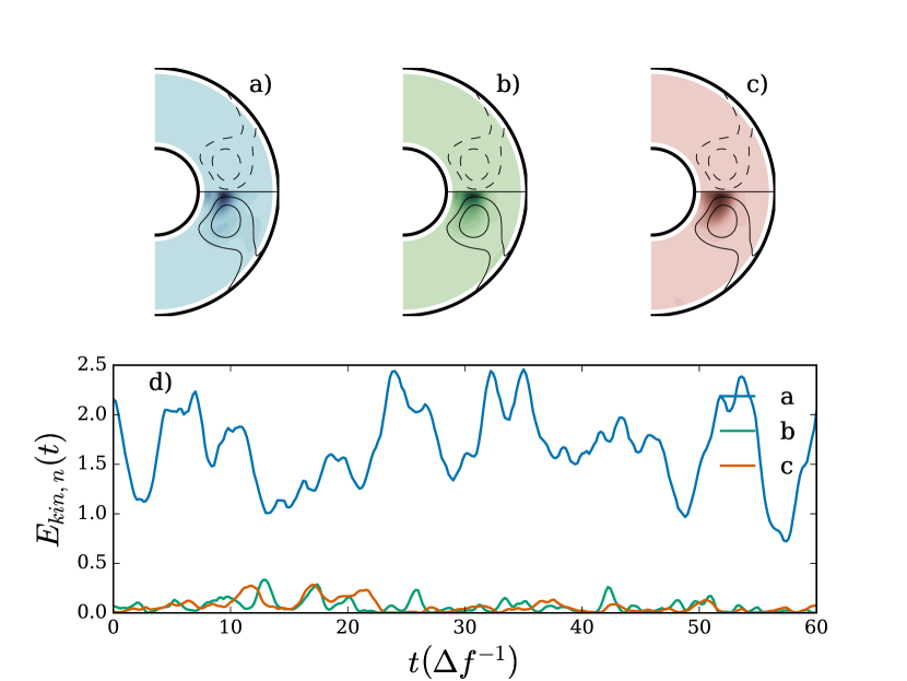
Figure 15: (a-c) Colormaps showing azimuthally averaged kinetic energy density of the first three singular modes of the $Ro=-1.0,\Lambda_{b}=0.190$ flow. The upper hemisphere shows the equatorially antisymmetric component of the mode; the lower hemisphere shows the equatorially symmetric component. (d) The energy in each mode (a-c) as a function of time, scaled against the mean energy in the kinetic fluctuations of the raw signal. Only the region $r\in[0.425,0.975]$ is included in the PCA.

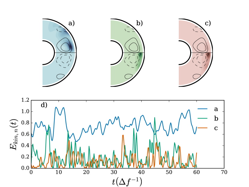
Figure 16: (a-c) Colormaps showing azimuthally averaged kinetic energy density of the first three singular modes of the $Ro=-1.2,\Lambda_{b}=0.190$ flow. The upper hemisphere shows the equatorially antisymmetric component of the mode; the lower hemisphere shows the equatorially symmetric component. (d) The energy in each mode (a-c) as a function of time, scaled against the mean energy in the kinetic fluctuations of the raw signal. Only the region $r\in[0.425,0.975]$ is included in the PCA.

Appendix B Simulation Parameters

The full simulations presented here were carried out using the nondimensional parameters and resolutions shown in Tab. 3. This table includes the magnetic Reynolds $\left(Rm\equiv r_{o}^{2}\Delta\Omega/\eta=Ro/Em\right)$ for comparison with other MHD simulations. Other works on MSC flow Hollerbach.RSPA.2009 were characterized by the Hartmann number $\left(Ha_{o,i}=r_{o,i}B_{o,i}/\sqrt{\mu\rho\nu\eta}\right)$ and Reynolds number $\left(Re=r_{o}^{2}\Delta\Omega/\nu\right)$, specifically because these numbers do not require that the outer sphere be rotating. Conveniently, the Ekman number is all that is required to convert into our nondimensionalization the rotation independent one $\left(Ha=\Lambda/\sqrt{Ek}\right.$, and $\left.Re=\left|Ro\right|/{\rm Ek}\right)$. This gives $10^{5}<Re<2\times 10^{6}$. The Hartmann number varies between $6<Ha_{o}<18$ at the outer sphere and $162<Ha_{i}<486$ at the inner sphere. In the physical experiment these values take the ranges $10^{6}<Re<2\times 10^{7}$, $Ha_{o}=195$, and $Ha_{i}=4430$.

		$\Lambda_{o}$	$\Lambda_{b}$	$Em$	$Rm$	$\ell_{max}$
$Ro$	$f_{o}$ (Hz)
-2.00	4.98	0.018	0.190	0.064	31.2	200
	9.97	0.009	0.095	0.032	62.5	200
	15.19	0.006	0.063	0.021	95.2	200
-1.75	4.98	0.018	0.190	0.064	27.3	200
	9.97	0.009	0.095	0.032	54.7	200
	15.19	0.006	0.063	0.021	83.3	200
-1.50	4.98	0.018	0.190	0.064	23.4	200
	9.97	0.009	0.095	0.032	46.9	200
	15.19	0.006	0.063	0.021	71.4	200
-1.20	4.98	0.018	0.190	0.064	18.8	200
	9.97	0.009	0.095	0.032	37.5	200
	15.19	0.006	0.063	0.021	57.1	200
-1.00	4.98	0.018	0.190	0.064	15.6	200
	9.97	0.009	0.095	0.032	31.2	200
-0.75	4.98	0.018	0.190	0.064	11.7	100
-0.50	4.98	0.018	0.190	0.064	7.8	100
	9.97	0.009	0.095	0.032	15.6	100
1.00	4.98	0.018	0.190	0.064	15.6	150
	9.97	0.009	0.095	0.032	31.2	150
1.50	4.98	0.018	0.190	0.064	23.4	150
	9.97	0.009	0.095	0.032	46.9	150

Table 3: Resolutions and nondimensional parameters of the simulations presented here. For all simulations the Ekman number $Ek=10^{-6}$ , the time resolution is $10^{-4}\Delta f^{-1}$, and the radial grid has 384 points. This table includes the magnetic Reynolds $\left(Rm\equiv r_{o}^{2}\Delta\Omega/\eta\right)$ for comparison with other MHD simulations. The corresponding outer sphere rotation frequency $f_{o}$ in Hz of the DTS-machine is also indicated.

Appendix C Principal Component Analysis of stable modes

Because the flows discussed in Section III.1 seem to primarily be saturated instabilities, they’re amenable to a principal component analysis (PCA), wherein the flow is decomposed into individual spatial modes, each with its own timeseries Abdi.CompStat.2010 . The modes are chosen to maximize the cross correlation in time between different measurements (here the kinetic and magnetic spectra at each radial gridpoint (i.e. the $s_{\ell,m}(r_{k}),t_{\ell,m}(r_{k}),S_{\ell,m}(r_{k})$ and $T_{\ell,m}(r_{k})$ of Eqn. 3). The analysis is carried in the frame of the inner sphere according to

$$\mathbf{A}=\mathbf{L}\mathbf{\Sigma}\mathbf{R}^{H}.$$ (9)

Here, $\mathbf{A}$ is a matrix representing spatio-temporal data; $\mathbf{R}$ is a matrix of so-called right eigenvectors, each representing a single spatial configuration that evolves together ($\mathbf{R}^{H}$ is the complex conjugate and transpose of the matrix $\mathbf{R}$); $\mathbf{L}$ is a matrix of so-called left eigenvectors, each representing the collective time evolution of its corresponding right eigenvector; and $\mathbf{\Sigma}$ is a diagonal matrix of singular values, each representing the relative strengths of the modes. The matrix $\mathbf{A}$ is computed by removing the means of the magnetic and velocity fluctuations $\left(\widetilde{\mathbf{b}}(r,\theta,\phi,t_{j})\;{\rm and}\;\widetilde{\mathbf{u}}(r,\theta,\phi,t_{j})\;{\rm respectively}\right)$, and the singular value decomposition (SVD) is carried out using numpy’s linear algebra module SCIPY .

The time series of Fig. 13c and d are generated by converting individual principle components $n$ back into a collection of snapshots $\mathbf{u}_{n}\left(t_{j}\right)$ by

$$\mathbf{u}_{n}\left(t_{j}\right)=l_{j,n}\;\sigma_{n}\;\mathbf{r}_{n},$$ (10)

where $\mathbf{r_{n}}$ is an individual column of $\mathbf{R}$, $l_{j,n}$ is an individual entry in $\mathbf{L}$, and $\sigma_{n}$ is the singular value of $n$.

References

- (1) A. Figueroa, N. Schaeffer, H.-C. Nataf, and D. Schmitt, “Modes and instabilities in magnetized spherical Couette flow,” Journal of Fluid Mechanics, vol. 716, pp. 445–469, 2 2013.
- (2) G. Dumas, Study of spherical Couette flow via 3-D spectral simulations: large and narrow-gap flows and their transitions. PhD thesis, California Institute of Technology, Pasadena, California (USA), 1991.
- (3) C. Egbers and H. Rath, “The existence of Taylor vortices and wide-gap instabilities in spherical couette flow,” Acta mechanica, vol. 111, no. 3-4, pp. 125–140, 1995.
- (4) Y. N. Belyaev, A. Monakhov, and I. Yavorskaya, “Stability of spherical couette flow in thick layers when the inner sphere revolves,” Fluid Dynamics, vol. 13, no. 2, pp. 162–168, 1978.
- (5) K. Nakabayashi, Z. Zheng, and Y. Tsuchida, “Characteristics of disturbances in the laminar–turbulent transition of spherical couette flow. 2. new disturbances observed for a medium gap,” Physics of Fluids (1994-present), vol. 14, no. 11, pp. 3973–3982, 2002.
- (6) P. S. Marcus and L. S. Tuckerman, “Simulation of flow between concentric rotating spheres. part 2. transitions,” Journal of Fluid Mechanics, vol. 185, pp. 31–65, 1987.
- (7) I. Proudman, “The almost-rigid rotation of viscous fluid between concentric spheres,” J. Fluid Mech., vol. 1, pp. 505–516, 1956.
- (8) K. Stewartson, “On almost rigid rotations,” J. Fluid Mech., vol. 1, pp. 131–144, 1966.
- (9) R. Hollerbach, “Instabilities of the Stewartson layer Part 1. The dependence on the sign of ,” Journal of Fluid Mechanics, vol. 492, pp. 289–302, 09 2003.
- (10) N. Schaeffer and P. Cardin, “Quasigeostrophic model of the instabilities of the Stewartson layer in flat and depth-varying containers,” Physics of Fluids, vol. 17, no. 10, p. 104111, 2005.
- (11) D. H. Kelley, S. A. Triana, D. S. Zimmerman, and D. P. Lathrop, “Selection of inertial modes in spherical Couette flow,” Phys. Rev. E, vol. 81, p. 026311, Feb 2010.
- (12) M. Rieutord, S. A. Triana, D. S. Zimmerman, and D. P. Lathrop, “Excitation of inertial modes in an experimental spherical Couette flow,” Phys. Rev. E, vol. 86, p. 026304, Aug. 2012.
- (13) J. Wicht, “Flow instabilities in the wide-gap spherical Couette system,” Journal of Fluid Mechanics, vol. 738, pp. 184–221, 12 2014.
- (14) E. Dormy, D. Jault, and A. M. Soward, “A super-rotating shear layer in magnetohydrodynamic spherical Couette flow,” Journal of Fluid Mechanics, vol. 452, pp. 263–291, Feb. 2002.
- (15) N. Kleeorin, I. Rogachevskii, A. Ruzmaikin, A. M. Soward, and S. Starchenko, “Axisymmetric flow between differentially rotating spheres in a dipole magnetic field,” Journal of Fluid Mechanics, vol. 344, pp. 213–244, 8 1997.
- (16) D. Brito, T. Alboussière, P. Cardin, N. Gagnière, D. Jault, P. La Rizza, J.-P. Masson, H.-C. Nataf, and D. Schmitt, “Zonal shear and super-rotation in a magnetized spherical Couette-flow experiment,” Phys. Rev. E, vol. 83, p. 066310, Jun 2011.
- (17) H.-C. Nataf, T. Alboussière, D. Brito, P. Cardin, N. Gagnière, D. Jault, and D. Schmitt, “Rapidly rotating spherical Couette flow in a dipolar magnetic field: An experimental study of the mean axisymmetric flow,” Physics of the Earth and Planetary Interiors, vol. 170, pp. 60–72, Sept. 2008.
- (18) D. Schmitt, T. Alboussière, D. Brito, P. Cardin, N. Gagnière, D. Jault, and H.-C. Nataf, “Rotating spherical Couette flow in a dipolar magnetic field: experimental study of magneto-inertial waves,” J. Fluid Mech, vol. 604, pp. 175–197, 2008.
- (19) S. Cabanes, N. Schaeffer, and H.-C. Nataf, “Magnetic induction and diffusion mechanisms in a liquid sodium spherical Couette experiment,” Phys. Rev. E, vol. 90, p. 043018, Oct 2014.
- (20) N. Schaeffer, “Efficient spherical harmonic transforms aimed at pseudospectral numerical simulations,” Geochemistry, Geophysics, Geosystems, vol. 14, pp. 751–758, Mar. 2013.
- (21) G. A. Glatzmaier and P. H. Roberts, “A three-dimensional convective dynamo solution with rotating and finitely conducting inner core and mantle,” Physics of The Earth and Planetary Interiors, vol. 91, no. 1-3, pp. 63 – 75, 1995. Study of the Earth’s Deep Interior.
- (22) H.-C. Nataf and N. Schaeffer, “8.06 - turbulence in the core,” in Treatise on Geophysics (Second Edition) (G. Schubert, ed.), pp. 161 – 181, Oxford: Elsevier, second edition ed., 2015.
- (23) R. Hollerbach, “Non-axisymmetric instabilities in magnetic spherical Couette flow,” Proc. R. Soc. London A, vol. 465, pp. 2003–2013, 2009.
- (24) C. Gissinger, H. Ji, and J. Goodman, “Instabilities in magnetized spherical Couette flow,” Phys. Rev. E, vol. 84, p. 026308, Aug. 2011.
- (25) The ratio of rotation rates, s, and Reynolds numbers previously reported in Gissinger.PRE.2011 contained typos. Private Communication.
- (26) J. Ahrens, B. Geveci, and C. Law, ParaView: An End-User Tool for Large Data Visualization, Visualization Handbook. Elsevier, 2005.
- (27) J. Vidal, D. Cébron, N. Schaeffer, and R. Hollerbach, “Magnetic fields driven by tidal mixing in radiative stars,” Monthly Notices of the Royal Astronomical Society, vol. 475, no. 4, pp. 4579–4594, 2018.
- (28) E. Herbert, P.-P. Cortet, F. Daviaud, and B. Dubrulle, “Eckhaus-like instability of large scale coherent structures in a fully turbulent von kármán flow,” Physics of Fluids, vol. 26, no. 1, p. 015103, 2014.
- (29) G. Brethouwer, P. Schlatter, Y. Duguet, D. S. Henningson, and A. V. Johansson, “Recurrent bursts via linear processes in turbulent environments,” Physical review letters, vol. 112, no. 14, p. 144502, 2014.
- (30) D. S. Zimmerman, S. A. Triana, H.-C. Nataf, and D. P. Lathrop, “A turbulent, high magnetic Reynolds number experimental model of Earth’s core,” Journal of Geophysical Research (Solid Earth), vol. 119, pp. 4538–4557, June 2014.
- (31) R. Hollerbach, M. Junk, and C. Egbers, “Non-axisymmetric instabilities in basic state spherical couette flow,” Fluid dynamics research, vol. 38, no. 4, pp. 257–273, 2006.
- (32) H. Abdi and L. J. Williams, “Principal component analysis,” Wiley Interdisciplinary Reviews: Computational Statistics, vol. 2, no. 4, pp. 433–459, 2010.
- (33) E. Jones, T. Oliphant, P. Peterson, et al., “SciPy: Open source scientific tools for Python,” 2001–.