Continuous-Time, Discrete-Event Simulation from Counting Processes

Abstract

This is a method for discrete event simulation specified by survival analysis. It presents a sequence of steps. First, hazard rates from survival analysis specify the rates of a set of counting processes. Second, those counting processes define a transition kernel. Third, there are four different ways to sample that transition kernel, including a first-principles derivation of exact stochastic simulation algorithms (ssa) in continuous time. This simulation allows time-dependent intensities which include both continuous and atomic components. Separating the steps involved makes a clear correspondence between mathematical formulation and algorithmic implementation.

¡ccs2012¿ ¡concept¿ ¡concept_id¿10010147.10010341.10010349.10010354¡/concept_id¿ ¡concept_desc¿Computing methodologies Discrete-event simulation¡/concept_desc¿ ¡concept_significance¿500¡/concept_significance¿ ¡/concept¿ ¡concept¿ ¡concept_id¿10010147.10010341.10010342.10010343¡/concept_id¿ ¡concept_desc¿Computing methodologies Modeling methodologies¡/concept_desc¿ ¡concept_significance¿300¡/concept_significance¿ ¡/concept¿ ¡concept¿ ¡concept_id¿10002950.10003648.10003688.10003694¡/concept_id¿ ¡concept_desc¿Mathematics of computing Survival analysis¡/concept_desc¿ ¡concept_significance¿300¡/concept_significance¿ ¡/concept¿ ¡concept¿ ¡concept_id¿10002950.10003648.10003700¡/concept_id¿ ¡concept_desc¿Mathematics of computing Stochastic processes¡/concept_desc¿ ¡concept_significance¿100¡/concept_significance¿ ¡/concept¿ ¡/ccs2012¿ [500]Computing methodologies Discrete-event simulation [300]Computing methodologies Modeling methodologies [300]Mathematics of computing Survival analysis [100]Mathematics of computing Stochastic processes Andrew J. Dolgert. 2016. Continuous-Time, Discrete-Event Simulation from Counting Processes

This work was supported by USDA-APHIS Cooperative Agreement No. 15-9200-0411-CA with Cornell University.

Author’s address: A. J. Dolgert, (Current address) Institute for Health Metrics and Evaluation, University of Washington.

1 Introduction

A continuous-time, discrete-event (ctde) simulation can be based on any one of a number of stochastic processes, including Generalized Semi-Markov Processes (gsmp) [Glynn (1989)], Generalized Stochastic Petri Nets (gspn) [Haas (2002)], or chemical stochastic processes [Gillespie (2007)] These processes vary in how they define state and how they specify the distribution of times at which each event will fire, but all of them have the remarkable property that the hazard rate of any event in a realization of the process will match the hazard rate of the distribution of times used to specify that event.

In their work on chemical stochastic processes, Anderson and Kurtz 2015 offer a construction of a stochastic process which can serve as an alternative method of ctde simulation. Because it uses counting processes as the basis for the construction, their work emphasizes the role of hazard rates in defining the process. As a result, certain forms of gsmp and gspn, those which avoid use of immediate events and simultaneous events, could be considered subclasses for the purposes of computation. The formalism of counting processes also offers the algorithmic advantage of a clear separation between defining a transition kernel and sampling that kernel.

Anderson and Kurtz present the more general stochastic process, here called competing clocks, as a step in derivation of stochastic processes for chemical simulation. Implications of the general stochastic process for specification and computation are unexplored. The goal of this article is to expand upon the competing clocks process by clarifying how its specification relates to survival analysis and to show how the machinery of counting processes translates into modular and efficient computational algorithms. The scope of this article is time-homogeneous, continuous-time simulation with discrete space because discrete state spaces simplify the conditions under which a specification guarantees a single next time step.

In order to demonstrate the power of the counting process formalism, these counting processes can have any regular distribution, including those for which the hazard rate can have both a continuous and atomic part. This will produce a novel generalization of Next Reaction Method and Direct Method exact stochastic simulation algorithms. Johansen points out that atomic intensities can be useful for data analysis, which makes them important for simulation from such data analysis Johansen (1983). Such estimates appear as Dirac functions in published models, for instance in Viet et al 2004. The Nelson-Aalen estimator of cumulative hazard rate is, itself, discontinuous. Addressing distributions which can contain discontinuities addresses simulations which contain both purely continuous and purely discontinuous distributions. Finally, the set of computable models include all regular distributions, so they are included for completeness.

Sec. 2 defines the stochastic process. Sec. 3 connects that specification with survival analysis. Two consequences of this definition are that implementation of a library to support these simulations can mirror the mathematics quite closely, Sec. 4, and that sampling techniques from discrete-event simulation and chemical simulation can be used together, Sec. 5. Comparisons with previous work will be discussed in the conclusion.

2 Competing Clocks Construction

Anderson and Kurtz present a stochastic process 2015, here called a competing clocks process. This section extends that work only by including atomic hazards. The stochastic process they derive as an intermediate result towards applications in chemistry will be shown in the next section to be the basis for a continuous-time discrete event simulation. This section has two steps, definition of a single clock process as a counting process with a time-dependent intensity, and then composition of multiple clock processes into a competing clocks process.

The clock process is a counting process, $N(t)$, which starts at $N(0)=0$ and is constant except of jumps of $dN=1$. If the time of the $k$th jump is labeled $R_{k}$, the interarrival time is $U_{1}=R_{1}$, $U_{k}=R_{k}-R_{k-1}$. A counting process is characterized by its intensity, which is a measure that assigns to every time a probability the clock will jump in the next interval, $dt$. The hazard rate is the probability of the next jump, given the condition that that next jump has not yet happened. The two will have the same value over a time interval between jumps, so they may be used interchangeably, but the intensity is the intensity of the clock process while the hazard rate is the hazard rate of the next jump.

A realization of a clock process is a complete set of jump times. At any time, $t$, the past of the process is a set of jump times for times less than $t$, and is called a path, $v^{1}$, of the set of paths of $N$. The clock process, as defined by Kurtz 1980, can also depend on another path, $z$, of an external stochastic process, $Z$, to represent the environment. Both are restricted to have a limit from the left and be continuous from the right, which is cadlag, and the filtration of the clock process is the history of both before a current time, $\mathcal{N}_{t\text{-}}^{1}=\sigma(N(s),Z(s),s<t)$.

The intensity, then, is a function adapted to this filtration which maps time and an element of $(v^{1},z)\in(N,Z)$ to a non-negative number. An intensity must be measurable and a.s. finite. It also cannot depend on the future, so it depends on the paths $v^{1}$ and $z$ only for times less than $t$. The intensity has a continuous part which is written as $\lambda(t,v^{1},z)$ and an atomic part, written using the Dirac delta function, $\delta$, as

$$p(t,v^{1},z)=\sum_{i}p_{i}(v^{1},z)\delta(t-t_{i}(v^{1},z)),$$ (1)

which implies each shock, $p_{i}(v^{1},z)$, happens at time, $t_{i}(v^{1},z)$. Both continuous and atomic parts of the intensity are predictable functions of the filtration.

The clock process can be defined in terms of the given intensity by stating that, for each jump time, $R_{k}$, using the notation $t\wedge R_{k}=\mbox{min}(t,R_{k})$,

$$M_{k}(t)=N(t\wedge R_{k})-\int_{0}^{t\wedge R_{k}}\lambda(s,v^{1},z)ds-\sum_{t_{i}<t\wedge R_{k}}p_{i}(v^{1},z)$$ (2)

is a martingale, such that $E[M_{k}(t+s)|\mathcal{N}_{t\text{-}}]=M_{k}(t)$.

Competing clocks are a set of clock processes, labeled $j=1,2\ldots$. For any single clock process, consider other clock processes as its external environment, so that any one of them can depend on a joint history of all clocks, expressed as the filtration $\mathcal{N}_{t\text{-}}=\sigma(N_{j}(s),s<t,\forall j)$. The paths $v$ are the paths of all of the set of clock processes. Anderson and Kurtz permit the competing clocks to depend not only on their joint history but also on an external environment, but this presentation will exclude it to focus sampling algorithms where the next stopping time can be determined entirely from the hazards.

As for the single clock process, the intensity must be a measurable function of the filtration, and the sum of the intensities must be a.s. finite. What links the clock processes together is that the intensity of each clock process is a measurable function of the paths of any of the clock processes. The system stopping times, $T_{n}$ are the set of all jump times of all clocks, $R_{k}^{j}$. No two clocks may jump at the same time, which means that no atomic jumps $t_{ij}(v)$ may be the same among all of the atomic intensities,

$$p_{j}(t,v)=\sum_{i}p_{ij}(v)\delta(t-t_{ij}(v)).$$ (3)

The definition of the competing clocks process is an assertion that

$$M_{nj}(t)=N_{j}(t\wedge T_{n})-\int_{0}^{t\wedge T_{n}}\lambda_{j}(s,v)ds-\sum_{t_{ij}<t\wedge T_{n}}p_{ij}(v)$$ (4)

is a martingale. This concise definition determines stochastic processes $N_{j}(t)$ from specifications for $\lambda_{j}$ and $p_{j}$. The next section discusses how to choose those specifications.

Notation	Description
$N_{j}(t)$	The $j$th lock process
$R^{j}_{k}$	The time of each jump for a clock process
$\lambda_{j}(t,v)$	Continuous intensity of clock process $j$
$p_{j}(t,v)$	Atomic intensity of clock process $j$
$h_{j}(t)$	Continuous hazard rate until the next jump of clock process $j$
$a_{j}(t)$	Atomic hazard rate until the next jump of clock process $j$
$\nu_{j}$	Jump mark for each clock process
$S_{j}(t)$	Survival of clock process $j$
$X(t)$	Discrete state of the system
$T_{n}$	Each stopping time of the system

3 Correspondence Between a Model and a Process

Given a specific set of functions for the intensity, Eq. 4 implies a stochastic differential equation which can then be solved as described in Sec. 5. What choices of $\lambda_{j}(t,v)$ and $p_{j}(t,v)$ are meaningful representations of disease progression, a financial system, or an influencer network? A model, in this case, is a set of rules about what can change next and the likelihood of a particular next change and time. This breaks down into two questions, what can happen and when it can happen.

The intensity of a clock process is written as a function of two variables, $t$ and $v$. The second variable is the set of jumps that have happened and times at which they happened, so it changes only at stopping times of the system. Assume $v$ is the history of the competing clocks up to some time $T_{n}$. The intensity can always be written as two functions. The function $\phi_{j}(v)$ looks at $v$ to determine whether this particular clock can fire and, if so, at what rate. The functions $h_{jn}(t)$ and $a_{jn}(t)$ specify the continuous and atomic hazard rate for process $j$ given the past at time $T_{n}$,

$$\phi_{j}:v \rightarrow (h_{jn}(t),a_{jn}(t))$$ (5)

$$h_{jn}:t \rightarrow \lambda_{j}(t,v)$$ (6)

$$a_{jn}:t \rightarrow p_{j}(t,v).$$ (7)

The first function, $\phi_{j}(v)$, determines what can happen. If a clock process can fire at some time in the future, according to the current $v$, then the hazard rate is nonzero somewhere. If a clock process cannot fire, then $\phi_{j}(v)$ maps to some other value, called $\Delta$, which indicates a jump is forbidden. The function $\phi_{j}(v)$ may return the same hazard rates for multiple stopping times of the whole system, so that the functional form of the hazard rates does not change. The most recent time at which a clock became enabled is its enabling time, $\mathcal{E}_{j}(v)$. Specification of the intensity of a clock process is specification of a sequence of hazard rates, each of which is a hazard rate given a certain past.

One reason to state discrete event simulation as competing clocks is to make an explicit connection to hazards estimated by survival analysis. The hazard rate in Eq.6 is for a single stochastic process. While this rate is applied to an individual clock process, it usually comes from observation of an ensemble of events. Aalen 2008 describes such survival analysis, which observes multiple instances of an event and treats each such event, $C_{j}$, with the same past, $\mathcal{N}_{t\text{-}}$, as having the same hazard rate,

$$\hat{h}(t)dt=P(t\leq C_{j}<t+dt|\mathcal{N}_{t\text{-}}).$$ (8)

A set of these events are grouped together into a stochastic process that counts those not fired,

$$Y(t)=\sum_{j}\mathcal{I}(C_{j}\leq t),$$ (9)

where the time is relative to a start time for each event, its enabling time. From this is constructed the intensity of a counting process that counts the number of events, $\hat{N}(t)$, which happen before time $t$,

$$\hat{\lambda}(t)dt=\hat{h}(t)Y(t)dt.$$ (10)

The integrated intensity is the predictable part of the counting process for the set of individual events,

$$E\left[\left.\hat{N}(t)-\int_{0}^{t}\hat{h}(s)Y(s)ds\right|\mathcal{N}_{t\text{-}}\right]=0.$$ (11)

This is the statistical model used to estimate hazard rates from observed outcomes. Survival analysis uses the aggregate of observed event times to estimate the unknown hazard rate, while the clock process uses known hazard rates to produce sequences of event times, so they are almost the reverse of each other, except that the Martingale in Eq. 11 is for an ensemble of the same event with sufficiently similar past, while the intensity for a single clock process is for a single event.

Representations of a model as a competing clocks process are not unique, but there is a most expanded representation, where there is a separate clock for each possible action in the system so that each clock process can jump at most once. For instance, $N$ individuals which could each make $k$ actions would have $kN$ clocks. If an individual could repeat actions, then there would be countably many clocks, but only a finite number of them could be enabled at any time. This would require that no jump by an enabled clock could cause more than a finite number of clocks to become enabled.

The hazard rates must match those estimated for the real-world processes in order for the competing clocks construction to be a faithful model. This is different from saying the specification must be explicitly in terms of hazard rates. Sometimes the specified rate for a clock process may be an Aalen-Johansen estimator, but it is more often a parametric distribution, such as a Gamma distribution or Weibull distribution, whose hazard rate matches an estimate. The hazard rates themselves are not a necessary computational tool for simulation. They are the measure by which the simulation conforms to observations.

The intensity must be locally finite between jumps of the system time $T_{n}$. The hazard rate could, for instance, be specified as a uniform distribution between $T_{a}$ and $T_{b}$. The hazard rate of the uniform distribution is infinite at $T_{b}$, but the stochastic process is realized by sampling from the hazard rate, so the jump time will always be before $T_{b}$, making the intensity locally finite.

Example: Rabbits Eating Create a Poisson-distributed clock process, $N_{0}(t)$, with rate $l$, which represents a count of food produced. It is always enabled. Each of $M$ rabbits has a set $K_{m}$ of clock processes which represent varying integral amounts of food, $d_{k}$, the rabbit might eat. A random variable representing uneaten food is the total amount of food produced minus the counts of all clock processes representing rabbit consumption,

$$d=N_{0}(t)-\sum_{m=1}^{|M|}\sum_{k\in K_{m}}N_{mk}(t)d_{k}$$ (12)

with multipliers to represent the amount consumed. Each eating process, $N_{mk}(t)$, has an enabling rule, $d_{k}>d$, so that one rabbit consuming food can disable eating processes for other rabbits at the jump time. The enabling time of any eating process always maps to the last time the rabbit ate as the maximum jump time of the eating processes for that rabbit. Call it $\mathcal{E}_{m}$. Let the intensity of the eating clocks have a Weibull-distributed interarrival time,

$$S_{j}(t)=1-\exp((-(t-\mathcal{E}_{m})/f)^{2})$$ (13)

where $f$ depends on the size of the last meal.

Each clock process has an enabling time which can map to infinity if an enabling rule is not met, and it has a hazard rate defined by supplying a known distribution. The net result of these stochastic process is an observable amount of uneaten food and rate at which the rabbits eat when competing for the food.

4 Computing a Realization

The competing clocks construction defines a model which produces unique, computable realizations. This section describes several arbitrary choices which are made for the sake of efficiency of computation and algorithmic clarity.

4.1 Natural algorithm to compute a realization

The minimum information needed to define a model is how each jump affects the intensity for each clock process. The filtration contains all of the information required because it is the $\sigma$-field of the paths of each of the clock processes. A cumulative intensity adapted directly to the filtration is called natural.

The algorithm to compute a realization will sample the next jump, $j^{\prime}$, and time, $T_{n}$, given the filtration at the previous jump, $T_{n-1}$. In terms of the minimum information, there are three steps to obtaining the next state and time of the stochastic process, given the past.

1. Compute the transition kernel. Sec. 5 will describe two versions of a transition kernel, both of which depend on the value of the intensity as a function of a current time and system path,

   $$(T_{n-1},v)\rightarrow(\lambda_{j}(t,v),p_{j}(t,v)).$$ (14)

2. Sample the jump time and jump mark for the next transition.

   $$(\lambda_{j}(t,v),p_{j}(t,v))\rightarrow(j^{\prime},T_{n})$$ (15)

3. Apply the transition function to update the path of the system.

   $$(T_{n-1},T_{n},v,j^{\prime})\rightarrow(T_{n},v^{\prime})$$ (16)

   Changing the filtration implies updating any random variables adapted to that filtration, such as cumulative intensities.

The natural algorithm does not need reference to a system state.

4.2 Discrete State

The state of the system is a random variable derived from the self-exciting filtration. As described by Anderson and Kurtz 2015, a compact definition of a discrete state is to associate with each clock process a vector $\nu_{j}$ which increments an initial state $X(0)$ as

$$X(t)=X(0)+\sum_{j}N_{j}(t)\nu_{j}.$$ (17)

The vectors, $\nu_{j}$, can be considered jump marks for the clock processes. There is no restriction that the vectors $\nu_{j}$ be unique.

In many cases, every intensity in the system is a function of the history only through the state. In the broadest case, every intensity could depend on the full path of the state, its value at every time in the past, as $\lambda_{j}(t,X(t))$. Other systems restrict the intensities to depend only on the most recent value of the state, some $X(T_{k})$, and the time at which the state entered that most recent value, $\lambda_{j}(t,X(T_{k}),T_{k})$. These kinds of restricted forms of the intensity depend on the structure of the analysis which produced the specifications for hazard rates. Each such restriction can reduce the amount of computational state required for a sampling algorithm.

4.3 Dependency graph

The intensity of any clock process will be a function of the paths of some subset of clock processes. This creates a directed graph from a clock process to those clock process whose jumps may affect its intensity. The dependency graph provides an efficient way to calculate which clocks’ intensities need to be re-evaluated after any clock fires. For some models, such as a susceptible-infectious-recovered (sir) model Allen (1994), a natural algorithm with a dependency graph may be the most efficient expression of the model.

Gibson and Bruck observed 2000 that if the form of the intensity is such that it is a function of the state, for instance $\lambda_{j}(t,X(T_{k}))$, then the dependency graph may be written as a directed, bipartite graph. The two types of nodes in the graph are substates of the state, $X=(x_{1},x_{2},x_{3}\ldots)$, and the clocks $N=(N_{1},N_{2},N_{3}\ldots)$. There is an edge from every substate to all clocks whose jumps would change that substate. There is an edge from every clock to all substates on whose path it depends. In most cases, a bipartite representation of the dependency graph will require less memory than a dependency graph among clock processes.

The dependency graph also serves as a form of parameterization of the clocks. When multiple individuals can have similar behavior, there will be cases where two clock intensities can be written as the same functional form applied to different substates,

$$\lambda_{1}(t,X(t)) = l(t,x_{1},x_{2})$$ (18)

$$\lambda_{2}(t,X(t)) = l(t,x_{3},x_{4}).$$ (19)

In this case, the specification of the intensity can be the common function, $l$, and projections of the state, defined by the dependency graph.

The reaction graph used in chemical simulation makes assumptions about the dependency graph and encodes more information. Reaction graphs annotate transitions, equivalent to clock processes, with rates and annotate edges with stoichiometric constants which are equivalent to the $\nu_{j}$. For chemical simulation, knowing the stoichiometric constants of a transition also defines enabling rules and parameterizes intensity functions.

In order for one clock jump to be the cause of another, there must be a path from one to the other in the dependency graph. It is the topology upon which the intensities define the dynamics. The dependency graph encodes much of the order of computation as a result. The number of nodes, the number of clocks, and the distribution of cardinalities of the clocks and nodes determine the number of instructions necessary to sample the next jump of a realization.

4.4 Finiteness

There are some expected requirements for finiteness. The number of enabled processes at any stopping time must be finite, both for representation on a computer and because the sampling algorithms in Sec. 5 rely on finite alternatives. The number of edges in the adjacency graph from one clock to substates and to other clocks must be finite, as well, because they will be checked for enabled clocks at each jump of the system.

More interesting is what need not be finite. The space of substates could be infinite. A common representation for the state is a map from an index to the substate, and setting a state to zero can be done by removing the substate from the map. In this way, a simulation of an ant could allow it to walk an infinite plane. Similarly, a stochastic process could be defined for an infinite number of clocks for which only a finite number are enabled at any time.

4.5 Stateful clock hazard rates

An important optimization is saving the hazard rates of clocks between jumps of the system. The intensity function was described in Eqs. 5–7 as having two parts, one which calculates a clock’s current hazard rate and the clock’s hazard rate which is a given function of time. The set of current hazard rates, $h_{jn}(t)$ and $p_{jn}(t)$, can be kept as computational state between jumps as long as that set is updated to account for additions, subtractions, or modifications to clock hazard rates. The hazard rates are not part of the minimum state of the stochastic equation because they are predictable functions of the history, $v$ or $X(t)$.

4.6 Computing a realization as a finite automaton

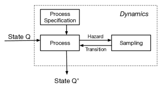
Figure 1: The core of a finite automaton to calculate a trajectory depends upon both the statistical process and its sampler.

This section organizes computation of a realization into the form of a stochastic finite automaton with no inputs and nondeterministic output. A sequential machine Arbib and Manes (1980) is a quintuple $(X_{0},Q,\delta,Y,\lambda)$, where $X_{0}$ is the input set, $Q$ the set of states, $\delta$ the dynamics, $Y$ the set of outputs, and $\lambda$ the output function. (The notation, $\lambda_{j}$, will refer below solely to clock intensities.) This section will describe the state and dynamics of that sequential machine.

The dynamics are a function from the state and input set to a new state, where the state, in this case, refers to all mutable state of the system, which is the discrete state $X(t)$, the current hazard rates, $h_{jn}(T_{n})$, and any state associated with sampling. The entities that define the dynamics are the space of the discrete states, the dependency graph, and the clock intensities. For each clock, specification includes an enabling function which returns also whether enabling has changed since the last discrete state, and, for each enabled clock, a function which returns its current hazard rate.

The three steps in Sec. 4.1 are the dynamics of the finite automaton. Written in terms of discrete state and caching of hazards, they become the following:

1. Compute the transition kernel.

   $$(T_{n-1},X(T_{n-1}))\rightarrow(h_{j,n-1}(t,X(T_{n-1})),a_{j,n-1}(t,X(T_{n-1})))$$ (20)

2. Sample the jump time and jump mark for the next transition.

   $$(h_{j,n-1}(t,X(T_{n-1})),a_{j,n-1}(t,X(T_{n-1})))\rightarrow(j^{\prime},T_{n})$$ (21)

3. Apply the transition function to update the state.

   $$(T_{n-1},X(T_{n-1}),\nu_{j},j^{\prime},T_{n})\rightarrow(T_{n},X(T_{n}),h_{j,n}(t,X(T_{n})),a_{j,n}(t,X(T_{n})))$$ (22)

   Applying the transition function requires using the dependency graph to update all hazard rates which change. During that update, the hazard rates, as a group, do not reflect the state of the system. Any derivative quantities, such as integrated hazard rates, need to be updated during this invariant-breaking step.

Output is separate from the dynamics and is a function of the filtration. The output observable of the sequential machine could be the filtration directly, $(T_{n},j)$, or the set of states and times, $(T_{n},X(T_{n}))$, or any random variable computed from these.

5 Sampling

5.1 First Reaction Method

The martingale definition of the competing clocks process, Eq. 4, is equivalent to a stochastic equation whose solution defines the transition kernel to sample. Take any of the clock processes, and label the survival of its interarrival time since its last jump at $R_{k-1}$ as $S_{j}(t)=P[R_{k}-R_{k-1}>t]$. Write the cumulative intensity as

$$\Lambda_{j}(t)=\int_{0}^{t}\lambda_{j}(s,v)ds+\sum_{t_{ij}<t}p_{ij}(v),$$ (23)

where $v$ is the path for all of the clock processes. The probability definitions for the survival and hazard relate the two as

$$dS_{j}(t)=-S_{j}(t^{-})d\Lambda_{j}(t),$$ (24)

where $S_{j}(t^{-})$ indicates the value of the survival just before time $t$. Eq. 24 is a Doléans-Dade differential relation whose solution is given by product integration Gill and Johansen (1990),

$$S_{j}(t)=e^{-\int_{R_{k-1}}^{t}\lambda_{j}(s,v)ds}\prod_{R_{k-1}<t_{i}\leq t}(1-p_{ij}(v)).$$ (25)

These are the distributions of jump times for each clock process to fire, were it the first to fire next. As such, they are called putative distributions.

The name competing processes comes from Markov renewal processes, where, at any time step $T_{n-1}$, the next jump of the process can be sampled by transforming the problem into $j$ separate distributions in time Howard (2007). The First Reaction Method for competing clocks substitutes, at a time $T_{n-1}$, the current hazard rate for the intensity, using $\phi_{j}(v)\mapsto(h_{j,n-1}(t),a_{j,n-1}(t))$. It then samples the distributions defined by these hazard rates to determine which clock process has the soonest jump time. Given independent uniform random numbers, $U_{j}\in[0,1)$, and cumulative distributions, $F_{j}(t)=1-S_{j}(t)$, the sampling algorithm is

$$t_{j}^{\prime}=F_{j}^{-1}(U_{j})\qquad T_{n}=\min(t_{j}^{\prime})$$ (26)

The algorithm chooses the minimum jump, updates intensities, and generates a fresh set of random numbers and putative firing times, $t_{j}^{\prime}$. Gillespie named this technique the First Reaction Method 1978, and it differs from classic competing processes in that more than one of the jumps may cause the system to enter the same state.

5.2 Next Reaction Method

Every sampling method for competing clocks samples a joint distribution over which clock jumps and when is the next jump. While the First Reaction Method samples at each time interval separately, the Next Reaction Method Gibson and Bruck (2000) examines each clock process separately, saving samples between times $T_{n}$. Justification for saving samples rests on proving that competing clocks processes are independent, doubly-stochastic Poisson processes.

Unit Poisson processes have the special property that repeated sampling for the next to fire from a set of Poisson processes can save the times of all samples that were later than the soonest Van Kampen (1992). Denote unit Poisson processes by $N_{\pi j}(\tau)$ and their cumulative distributions by $F_{\pi j}(\tau_{j})=1-e^{-\tau_{j}}$. Generate putative firing times, $\tau_{j}^{\prime}=F_{\pi j}^{-1}(U_{j})$, where $U_{j}\in[0,1)$. After selecting the next time as $T_{n}=\mbox{min}(\tau_{j}^{\prime})$ and removing it from the set of times, subtract $T_{n}$ from the remaining $\tau_{j}^{\prime}$. The distribution of $\tau_{j}^{\prime}$ will still be exponentially-distributed and can be used to choose the next soonest time. The Next Reaction Method applies this same technique to a situation where each Poisson process has a clock which is itself a stochastic variable.

Kallenberg 1990 showed that it is possible to write a clock process as a unit Poisson process which depends on a time process,

$$L_{j}(t,v)=\int_{0}^{t}\lambda_{j}(s,v)ds+\sum_{0<t_{i}\leq t}\ln(1-p_{ij}(v)).$$ (27)

Then the clock process is explicitly doubly-stochastic,

$$N_{j}(t,v)=N_{\pi j}(L_{j}(t,v)).$$ (28)

One way to see that Eqs. 28 and 25 are equivalent is to compute Eq. 24 for the clock process,

$$dS_{\pi j}(L_{j}(t,v))=-S_{\pi j}(L_{j}(t,v))d\Lambda_{j}(t,v),$$ (29)

which means that $S_{\pi j}(L(t,v))$ has the same infinitesimal generator as $N_{j}(t,v)$, so it has the same survival. When the intensity is purely continuous, the time process coincides with the integrated intensity. In the more general case including atomic contributions, the integrated intensity is different from the time process.

Aalen and Hoem proved that sampling doubly-stochastic processes with continuous hazards doesn’t introduce bias, despite explicit dependence on each other through $v$ 1978. Extension of independence among the unit Poisson processes to time processes of discontinuous cumulative intensity was remarked to be an open question Vere-Jones and Schoenberg (2004). As is sometimes the case, the computational framework proposed here will rest upon a result which is reasonable and seen to work although it is unproven.

Saving the $\tau_{j}^{\prime}$ from one step to the next is equivalent to saving $S_{j}^{\prime}=1-U_{j}=\exp(-\tau_{j}^{\prime})$ from one step to the next. Each clock process, from the start of the simulation, has a sampled survival, $S_{j}^{\prime}$, and, whenever that clock process is enabled, it consumes from that survival at a rate given by $L_{j}(t,v)$ until it fires. Aalen and Hoem’s work gives permission to save $S_{j}^{\prime}$ from one jump to the next, as long as each step removes and resamples the $S_{j}^{\prime}$ of only the process that jumps. All variations on the Next Reaction Method are different ways to maintain the set of survivals given the need, at each time step, to find the minimum of the $t_{j}^{\prime}$ and then update the time processes when $v$ now includes a new jump and time.

Gibson and Bruck’s algorithm labels with $t_{i}$ those stopping times when $\phi_{j}(z)$ changes for some clock process $j$ 2000. The conditional survival is the survival to some $t_{2}$ given that the process survived to $t_{1}$, and it is multiplicative, so that $S_{j}(t)=S_{j0}(\mathcal{E}_{j}(v),t_{1})S_{j1}(t_{1},t)$ if the process survived past a time $t_{1}$. When a clock process is first enabled, sampling by inversion solves

$$S_{j}^{\prime}=S_{j0}(\mathcal{E}_{j}(v),t^{\prime})$$ (30)

for $t^{\prime}$. If the functional form changes at a stopping time $t_{1}$ before the clock has jumped, the Next Reaction Method rewrites the original inversion equation as

$$S_{j}^{\prime}=S_{j0}(\mathcal{E}_{j}(v),t_{1})S_{j1}(t_{1},t^{\prime}),$$ (31)

which uses the property that the survival is multiplicative. This is called shifting the distribution. Labeling the enabling time as $t_{0}=\mathcal{E}_{j}(v)$, the general form is

$$S_{j}^{\prime}=S_{jn}(t_{n},t^{\prime})\prod_{m=0}^{n-1}S_{jm}(t_{m},t_{m+1})$$ (32)

Gibson and Bruck’s version of the Next Reaction Method maintains the value of

$$S_{jn}^{\prime}=S_{j}^{\prime}/\prod_{m=0}^{n-1}S_{jm}(t_{m},t_{m+1})$$ (33)

as computational state with which to solve $S_{jn}^{\prime}=S_{jn}(t_{n},t^{\prime})$.

The survival can also be written in terms of the time process, and, working with a continuous form of the time process, Anderson showed 2007 that its conditional form

$$L_{j}(t_{1},t_{2},v)=\int_{t_{1}}^{t_{2}}h_{j}(s)ds+\sum_{t_{1}<t_{i}\leq t_{2}}\ln(1-a_{ij}).$$ (34)

will express the Next Reaction Method as an additive rule,

$$\ln(S_{j}^{\prime})=L_{jn}(t_{n},t_{j}^{\prime},v)+\sum_{m=0}^{n-1}L_{jm}(t_{m},t_{m+1},v).$$ (35)

The running value of the second term is saved as $L_{jn}^{\prime}$. For some distributions, such as the exponential and Weibull distributions, this algorithm is involves only addition instead of exponentials, making it preferable to Gibson and Bruck’s formulation.

The algorithm for the Next Reaction Method can choose whether to update resampled jump times using the survival, Eq. 32, or the time process, Eq. 35, depending on which is most efficient for the distribution of a particular clock’s next jump. Any distribution used in a simulation needs to support three operations.

1. The first sample need not use inversion, but it must return the survival of the draw,

   $$S_{j0}(t),\mbox{rng}\rightarrow(t_{j}^{\prime},S_{j}^{\prime})$$ (36)

   or the log of the survival,

   $$S_{j0}(t),\mbox{rng}\rightarrow(t_{j}^{\prime},\ln(S_{j}^{\prime})),$$ (37)

   depending on whether conditional survival or time process will be used.

2. Later samples must match the survival of the initial draw, usually using sampling by inversion,

   $$(S_{jn}(t_{n},t),S_{jn}^{\prime})\rightarrow t_{j}^{\prime}\ \mbox{or}\ (L_{jn}(t_{n},t),\ln(S_{jn}^{\prime}))\rightarrow t_{j}^{\prime}$$ (38)

   Distributions without an analytic inverse require numerical inversion.

3. Each distribution must also calculate the cumulative survival or cumulative time process, given a time interval over which the associated clock has not fired,

   $$(S_{j,n}(t_{n},t),T_{n})\rightarrow S_{jn}^{\prime}\ \mbox{or}\ (L_{j,n}(t_{n},t),T_{n})\rightarrow L_{jn}^{\prime}.$$ (39)

By exploiting the similarity between the survival and hazard techniques, it is possible to create a single interface which permits sampling any distribution with the most appropriate technique.

5.3 Next to Fire

Part of the definition of the Generalized Semi-Markov Process (gsmp) is how to sample it Glynn (1989). The method is to sample all enabled clocks, select the soonest, and then resample those which were affected by the soonest. If a clock is non-exponential, or if its exponential rate has changed, then resample the clock with a shifted distribution, just as in the Next Reaction Method. What differs from the Next Reaction Method is that there is no effort to resample using the same cumulative survival.

The chief disadvantage is that resampling requires generation of a new random number, which is now a relatively less expensive operation than it once was. The great advantage for computational efficiency is that there is more choice in how to sample given distributions. There are stability advantages to sampling by inversion, but using sampling methods specific to distributions can be much faster. Sampling non-exponential continuous distributions requires care. A panoply of techniques are covered in Devroye 1986, and methods for automatic generation are discussed by Hörmann et al. who have written a software library, unu.ran, which which calculates distributions using several methods for inversion while providing calculation of the conditional survival Hörmann and Leydold (2000).

For sampling, distributions which are are both continuous and atomic form a mixture model. Sampling continuous distributions by composition techniques breaks the problem into a discrete choice over mixture components and then continuous sampling within the component.

While numerical inversion and integration of distributions can be time-consuming, the central object of Next to Fire algorithms is the calculation of the clock process whose next jump time is soonest. The dependency graph controls which jump times are added, removed, or modified in a set of putative jump times. Using this graph to speed updates is the second contribution to computational efficiency. The computer science name for this algorithm is an indexed arg min, or an indexed arg max with an objective function which is $-t_{j}$. The most common data structure for storing putative times is an indexed heap. While the Fibonacci heap has the best order of computation for large simulations, pairing heaps have better performance in most cases and are significantly simpler to implement correctly Mauch and Stalzer (2011).

5.4 Direct Methods

The previous three sampling techniques took independent samples of the clock processes. The class of direct methods constructs the joint density of the next clock to jump and time at which it jumps in order to make only two samples at each step of a realization.

The result for purely continuous hazard rates is well-known, and the result can be obtained in general from Jacod’s theorem Jacod (1975). Appendix APPENDIX: Derivation of Competing Risks for Discontinuous Hazards derives competing risks for discontinuous cumulative hazards. The survival in the current state is

$$P[T_{n}>t]=\exp\left[{-\int_{T_{n-1}}^{t}\sum_{j}h_{j}(s)ds}\right]\prod_{T_{n-1}<t_{j}\leq t,\forall j}(1-p_{0j}(t)).$$ (40)

and the cumulative incidence function is

$$P[T_{n}\leq t,J=h]=\int_{T_{n-1}}^{t}P[T_{n}>s]h_{j}(s)ds+\sum_{T_{n-1}<t_{j}\leq t,\forall j}P[T_{n}>t-]p_{j}(u).$$ (41)

The cumulative incidence function is a joint distribution over the discrete set of clock processes and the continuous time for the next event. The direct method samples this joint distribution using the method of conditional probability, which takes the density, separates it into marginal and conditional, and samples first the marginal, then the conditional.

The density of Eq. 41 is called the the cause-specific density,

$$dQ(j,t)=P[T_{n}>t]h_{j}(t)dt+P[T_{n}>t-]p_{j}(t).$$ (42)

The waiting time factorization marginalizes over the $j$ to produce a waiting time, $dW(t)=\sum_{j}dQ(j,t)$, and a conditional stochastic matrix, $\pi_{j}(t)$. Algorithms which sample the waiting time factorization are called direct methods, and they proceed in two steps. First sample the waiting time density,

$$U_{1}^{\prime}=\int_{0}^{t^{\prime}}dW(s)=P[T_{n}<t^{\prime}]$$ (43)

and then sample the stochastic matrix given that time for the smallest $j^{\prime}$ such that

$$U_{2}^{\prime}\leq\sum_{j=1}^{j^{\prime}}\pi_{j}(t^{\prime}).$$ (44)

Sampling for $\tau^{\prime}$ tells us will either return a unique atomic hazard, which immediately tells us which clock jumped, or it returns a continuous hazard, for which

$$\pi_{j}(t^{\prime})=\frac{h_{j}(t^{\prime})}{\sum_{k}h_{k}(t^{\prime})}$$ (45)

permits a discrete draw over the clocks.

Given that the cause-specific density has two variables, there is a second factorization, rarely used for computation, called the holding time factorization. It entails calculating the marginal over times,

$$\pi_{j}=\int_{0}^{\infty}dF=P[T_{n}<\infty,J=j),$$ (46)

which is just the stochastic matrix. The holding time is a probability for a jump to a state given that the state is already decided, $dF(j,t)/\pi_{j}$. For exponential distributions, the holding time and waiting time factorizations are indistinguishable.

Stating the waiting time as the sample of a univariate distribution, as in Eq. 43, reduces computation to a standard set of techniques covered by sampling theory, with the additional optimization that the set of hazards remain consistent from jump to jump, except as enabled, disabled, or modified according to the dependency graph.

Were all of the hazards constant, the problem reduces to calculation of the sum $\sum_{j}h_{j}(t)$ given updates to the list of enabled hazards. Further, Eq. 45 relies on partial sums of hazards. Algorithms to maintain partial sums of a mutable list are called prefix sum algorithms and are covered nicely by Blelloch Blelloch (1990). For instance, a binary heap can quickly calculate prefix sums for a system with a constant total number of enabled clocks. While different methods for the partial sum algorithm have spawned different names within the chemical simulation community, they represent a well-contained point of variation for an implementation, and the range of choices are explored in an encyclopedic paper Mauch and Stalzer (2011).

For non-exponential continuous hazards, the Eq. 43 requires inversion of the sum of hazard functions. For certain distributions, such as Weibull, this inversion may be analytic. In most cases, it is not. Direct integration may be practical for small problems on many-core architectures, but rejection-based algorithms can avoid integration. Thanh and Priami use a composition-rejection algorithm for hazards of chemical processes, constructing a piecewise-linear envelope Thanh and Priami (2015), and Holubec applies what Devroye calls the thinning method, which is exact for bounded hazards Holubec et al. (2011).

5.5 Hierarchical

Given the possibility that some clock processes are exponentially-distributed, some atomic, and some non-exponential, all within the same simulation, hierarchical sampling methods can be important for efficiency. There are two different kinds of hierarchical methods for exact simulation and the choice among these methods depends on model size, the structure of the dependency graph, and types of distributions for sets of clocks to most appropriate sampling algorithms Mauch and Stalzer (2011).

Direct methods which sample the waiting time factorization must sample by inversion a sum of hazard rates. Because a sum of sums is itself a sum, it is common to group hazards according to special properties which make sums easier to compute. For instance, a set of constant hazards, all with the same value, can be represented by a binary tree over integers. There may be sets of hazards which are updated together, amortizing time for modification of cumulative sums.

Similarly, sampling independent Poisson processes by the Next Reaction Method or the Next to Fire method finds the soonest to jump among all clocks. Some subset of clocks can use a direct method. Others can use a first reaction method. Then the minimum time of all putative times is the next jump.

6 Conclusion

Competing clocks model a broad class of simulations. They can be understood by comparison with the two most similar techniques, chemical simulation and the gspn.

Chemical simulation in continuous time has a discrete space of reactants, which are chemical components Gillespie (2007); Gibson and Bruck (2000). It establishes a separate stochastic process in continuous time for each possible reaction of those reactants, and the reaction rates are hazard rates, called propensities. They depend on the current state, $X(t)$. While competing clocks are defined on jump times, with the state as a predictable variable, the state of the system in chemical simulation is the state of the reactants and interarrival times of the reactions. Time-dependence in hazard rates tends to come from time-inhomogeneous constraints, such as changing the volume of a container. How an intensity might depend on the path of $X(t)$ is less relevant for this physical system. Chemical simulation can make a set of assumptions which are a special case of competing clocks.

The gspn is built around the transition from a state $s$ to a new state $s^{\prime}$, whereas the insight of Anderson and Kurtz is to build competing clocks from the path of events and how it defines a transition kernel. Built into the definition of the gspn is how to sample clock readings, whereas that is a distinct question for competing clocks. Nevertheless, likelihood of a realization of both processes, given the same specification, takes the same form. In general, the gspn is a more thorough tool for engineering simulation because techniques for immediate events and simultaneous events are appropriate for models of management and human-designed automation.

The clock-setting distribution of a gspn is the distribution generated by the hazard rate of that event. It is defined as a function of four quantities for the gspn, the previous state, the most recent state which enabled the distribution, the event that caused that state, and the event that is enabled. For competing clocks, the hazard rate can depend on any part of the filtration, or variable derived from the filtration, since the last time that clock fired, because each clock process is regenerative. If a clock just fired and is being reenabled, then it cannot depend on anything but the current state. On the other hand, if a clock has been disabled for some time since it last fired, or since the simulation began, then it can depend on any part of the filtration since that time.

In contrast to both chemical simulation and the gspn, competing clocks have no useful mechanism for specification of which clock is enabled or disabled after a transition. That decision is made by a specified function, $\phi_{j}(v)$, for which the other two offer a more structured approach. This does allow, however, for other ways to specify the causal chain of what enables and disables events.

Writing a simulation with competing clocks is remarkably direct. The state, if there is one, must be a map from a key to a state value. Each clock process is defined by three things. The enabling function looks at the state and says yes or no. There can be some stateful memory because the intensity can depend on the path of the system, so the intensity function looks at both the current state and whatever it has saved from past observations in order to generate a distribution for when the clock will putatively jump. The firing function of the intensity is just a vector of how it changes the discrete state. If a dependency graph is used, then these functions can be parameterized by which states neighbor the clock process on the dependency graph.

Sampling of the process is separate from statement of a particular clock process, much like in chemical simulation. As a result, it is possible to build a library with which to build optimized simulations of clock processes. The authors have contributed such a library, written in the Julia language, using unu.ran for generation of random variates Dolgert (2016).

Extensions to the clock processes, as presented here, would not hinder the connection to survival analysis. For instance, Aalen discusses counting processes on continuous state spaces Aalen et al. (2008). This article excluded the use of a process, $Z$, to represent the external environment because it introduces the complication, in Eq. 5, that $\phi_{j}(v,z)$ would need to allow for the path, $z$, to modify its output hazard rate at times before the next stopping time sampled by the kernel. If the external environment is treated as a known quantity before the simulation, its inclusion is trivial. If it is treated as a stochastic input, it changes sampling methods significantly.

Also, as mentioned earlier, instantaneous transitions are a known convenience. In addition, the jump of a single clock could be the marginal sample for a conditional sample among multiple outcomes. A hierarchical sampling strategy can reduce the order of computation significantly in some cases.

APPENDIX: Derivation of Competing Risks for Discontinuous Hazards

Aalen derives competing risks in continuous time using a product integral formulation Aalen et al. (2008). This derivation follows the same method using regular distributions. It is modeled by constructing the transition matrix, $\mathbf{P}(t|s)$ for times $s$ and $t$, in terms of the cumulative hazard matrix, $\mathbf{H}(t)$. Consider a system with an initial state $0$ and final states $(j=1,2,3,\cdots)$. We will write equations as though there were two final states, but it generalizes to countably many. The hazard matrix for the continuous part is

$$dH_{c}=\begin{array}[]{ccc}-\sum h_{j}(t)&h_{1}(t)&h_{2}(t)\\ 0&1&0\\ 0&0&1\end{array}.$$ (47)

The hazard matrix for the atomic part is nonzero only when one of the atomic jumps is nonzero, so it takes the form of delta functions as in Eq. 1,

$$dH_{a}=\begin{array}[]{ccc}-\sum p_{j}(t)&p_{1}(t)&p_{2}(t)\\ 0&1&0\\ 0&0&1\end{array}.$$ (48)

In product integral form, this matrix equation for the survival is

$$\mathbf{P}(t|s)=\Prodi_{s}^{t}(1-d\mathbf{H}),$$ (49)

which tells us that the only nonzero components of the transition matrix are in the first row,

$$P(t|s)=\begin{array}[]{ccc}P_{0}(t|s)&P_{1}(t|s)&P_{2}(t|s)\\ 0&1&0\\ 0&0&1\end{array},$$ (50)

so we can solve for the transition matrix in two steps, avoiding direct calculation of the product integral. The survival in the current state, $P_{0}(t)=P[T>\tau]$, can be formulated as a univariate transition whose cumulative intensity is the sum of each of the cause-specific intensities. Its value is

$$P_{0}(t|s)=e^{-\int_{s}^{t}\sum_{j}h_{j}(s)ds}\prod_{s<t_{j}\leq t,\forall j}(1-p_{j}(t)).$$ (51)

For transition to any other state, the Kolmogorov forward equation gives the transition matrix in terms of the survival and the hazard,

$$dP_{j}(t|s)=-P_{0}(t-)dH_{j}(t)$$ (52)

which makes the cumulative incidence function, $P[T\leq\tau,J=h]$

$$P_{j}(t|s)=\int_{s}^{t}P_{0}(s)h_{j}(s)ds+\sum_{s<t_{j}\leq t}P_{0}(t-)p_{j}(t).$$ (53)

For Markov systems, the cumulative incidence function is called the semi-Markov matrix. Note that the survival appears as a limit from below so that the atomic contribution at $t$ is not included in $P_{0}(t-)$.

The author would like to thank David Schneider and Chris Myers of Cornell University for advice and support.

Month YearMonth Year

References

- (1)
- Aalen et al. (2008) Odd Aalen, Ornulf Borgan, and Hakon Gjessing. 2008. Survival and event history analysis: a process point of view. Springer Science & Business Media. DOI:http://dx.doi.org/10.1007/978-0-387-68560-1
- Aalen and Hoem (1978) Odd O Aalen and Jan M Hoem. 1978. Random time changes for multivariate counting processes. Scandinavian Actuarial Journal 2 (1978), 81–101. DOI:http://dx.doi.org/10.1080/03461238.1978.10419480
- Allen (1994) Linda JS Allen. 1994. Some discrete-time SI, SIR, and SIS epidemic models. Mathematical biosciences 124, 1 (1994), 83–105. DOI:http://dx.doi.org/10.1016/0025-5564(94)90025-6
- Anderson (2007) David F Anderson. 2007. A modified next reaction method for simulating chemical systems with time dependent propensities and delays. The Journal of chemical physics 127, 21 (Dec. 2007), 214107. http://www.ncbi.nlm.nih.gov/pubmed/18067349
- Anderson and Kurtz (2015) David F Anderson and Thomas G Kurtz. 2015. Stochastic analysis of biochemical systems. Vol. 1. Springer. DOI:http://dx.doi.org/10.1007/978-3-319-16895-1
- Arbib and Manes (1980) Michael A Arbib and Ernest G Manes. 1980. Machines in a category. Journal of Pure and Applied Algebra 19 (1980), 9–20.
- Blelloch (1990) Guy E Blelloch. 1990. Prefix sums and their applications. (1990).
- Devroye (1986) Luc Devroye. 1986. Non-uniform random variate generation. Springer-Verlag, New York, New York, USA. DOI:http://dx.doi.org/10.1007/978-1-4613-8643-8
- Dolgert (2016) Andrew J Dolgert. 2016. CTDE: Continuous-time discrete event simulation. (Sept. 2016). Retrieved October 10, 2016 from https://github.com/adolgert/CTDE.jl
- Gibson and Bruck (2000) Michael A. Gibson and Jehoshua Bruck. 2000. Efficient Exact Stochastic Simulation of Chemical Systems with Many Species and Many Channels. The Journal of Physical Chemistry A 104, 9 (mar 2000), 1876–1889. DOI:http://dx.doi.org/10.1021/jp993732q
- Gill and Johansen (1990) Richard D Gill and Søren Johansen. 1990. A Survey of Product-Integration with a View Toward Application in Survival Analysis. The Annals of Statistics 18, 4 (1990), 1501–1555. http://www.jstor.org/stable/2241874
- Gillespie (1978) Daniel T. Gillespie. 1978. Monte Carlo simulation of random walks with residence time dependent transition probability rates. J. Comput. Phys. 28, 3 (sep 1978), 395–407. DOI:http://dx.doi.org/10.1016/0021-9991(78)90060-8
- Gillespie (2007) Daniel T. Gillespie. 2007. Stochastic simulation of chemical kinetics. Annual review of physical chemistry 58 (Jan. 2007), 35–55. http://www.annualreviews.org/doi/abs/10.1146/annurev.physchem.58.032806.104637
- Glynn (1989) P.W. Glynn. 1989. A GSMP formalism for discrete event systems. Proc. IEEE 77, 1 (1989), 14–23. DOI:http://dx.doi.org/10.1109/5.21067
- Haas (2002) Peter J. Haas. 2002. Stochastic Petri Nets: Modelling, Stability, Simulation. Springer-Verlag, New York, New York, USA. 509 pages. DOI:http://dx.doi.org/10.1007/b97265
- Holubec et al. (2011) V. Holubec, P. Chvosta, M. Einax, and P. Maass. 2011. Attempt time Monte Carlo: An alternative for simulation of stochastic jump processes with time-dependent transition rates. EPL (Europhysics Letters) 93, 4 (feb 2011), 40003. DOI:http://dx.doi.org/10.1209/0295-5075/93/40003
- Hörmann and Leydold (2000) Wolfgang Hörmann and Josef Leydold. 2000. Random-number and random-variate generation: automatic random variate generation for simulation input. In Proceedings of the 32nd conference on Winter simulation. Society for Computer Simulation International, 675–682. DOI:http://dx.doi.org/10.1109/wsc.2000.899779
- Howard (2007) Ronald A. Howard. 2007. Dynamic Probabilistic Systems: Semi-Markov and Decision Processes. Dover, Mineola, NY.
- Jacod (1975) Jean Jacod. 1975. Multivariate point processes: predictable projection, Radon-Nikodym derivatives, representation of martingales. Probability Theory and Related Fields 31, 3 (1975), 235–253. DOI:http://dx.doi.org/10.1007/bf00536010
- Johansen (1983) Søren Johansen. 1983. An extension of Cox’s regression model. International Statistical Review/Revue Internationale de Statistique (1983), 165–174. DOI:http://dx.doi.org/10.2307/1402746
- Kallenberg (1990) Olav Kallenberg. 1990. Random time change and an integral representation for marked stopping times. Probability Theory and Related Fields 86, 2 (1990), 167–202. DOI:http://dx.doi.org/10.1007/BF01474641
- Kurtz (1980) Thomas G Kurtz. 1980. Representations of Markov Processes as Multiparameter Time Changes. The Annals of Probability 8, 4 (1980), 682–715. DOI:http://dx.doi.org/10.1214/aop/1176994660
- Mauch and Stalzer (2011) Sean Mauch and Mark Stalzer. 2011. Efficient formulations for exact stochastic simulation of chemical systems. IEEE/ACM transactions on computational biology and bioinformatics / IEEE, ACM 8, 1 (2011), 27–35. DOI:http://dx.doi.org/10.1109/TCBB.2009.47
- Thanh and Priami (2015) Vo Hong Thanh and Corrado Priami. 2015. Simulation of biochemical reactions with time-dependent rates by the rejection- based algorithm. The Journal of Chemical Physics 143, 054104 (2015). DOI:http://dx.doi.org/10.1063/1.4927916
- Van Kampen (1992) Nicolaas Godfried Van Kampen. 1992. Stochastic processes in physics and chemistry. Vol. 1. Elsevier.
- Vere-Jones and Schoenberg (2004) David Vere-Jones and Frederic Paik Schoenberg. 2004. Rescaling Marked Point Processes. Australia & New Zealand Journal of Statistics 46, 1 (2004), 133–143. DOI:http://dx.doi.org/10.1111/j.1467-842X.2004.00319.x
- Viet et al. (2004) Anne-France Viet, Christine Fourichon, Henri Seegers, Christine Jacob, and Chantal Guihenneuc-Jouyaux. 2004. A model of the spread of the bovine viral-diarrhoea virus within a dairy herd. Preventive veterinary medicine 63, 3-4 (May 2004), 211–36. http://www.ncbi.nlm.nih.gov/pubmed/15158572