Optimizing Epistemic Model Checking using Conditional Independence

Abstract

Conditional independence reasoning has been shown to be helpful in the context of Bayesian nets to optimize probabilistic inference, and related techniques have been applied to speed up a number of logical reasoning tasks in boolean logic by eliminating irrelevant parts of the formulas. This paper shows that conditional independence reasoning can also be applied to optimize epistemic model checking, in which one verifies that a model for a number of agents operating with imperfect information satisfies a formula expressed in a modal multi-agent logic of knowledge. An optimization technique is developed that precedes the use of a model checking algorithm with an analysis that applies conditional independence reasoning to reduce the size of the model. The optimization has been implemented in the epistemic model checker MCK. The paper reports experimental results demonstrating that it can yield multiple orders of magnitude performance improvements.

1 Introduction

Epistemic model checking [14] is a technique for the verification of information theoretic properties, stated in terms of a modal logic of knowledge, in systems in which multiple agents operate with imperfect information of their environment. It has been applied to settings that include diagnosis [8], and reasoning in game-like settings [15, 16, 32], concurrent hardware protocols [3] and security protocols [1, 7, 31].

In dealing with imperfect information, the models of epistemic model checking can be viewed as a discrete relative of probabilistic models. The Bayesian net literature has developed some very effective techniques for the optimization of probabilistic reasoning based on the elimination of variables and conditional independence reasoning [19, 24]. Similar ideas have been shown to be applicable to reasoning in propositional logic [11].

The contribution of the present paper is to demonstrate that these conditional independence techniques from the Bayesian Net literature can also be applied in the context of epistemic model checking. We develop a generalization of these techniques for a multi-agent modal logic of knowledge, that enables model checking computations for this logic to be optimized by reducing the number of variables that need to be included in data structures used by the computation.

In epistemic model checking, one represents the model as a concurrent program, in which each of the agents executes a protocol in the context of an environment. We provide a symbolic execution method for generating from this concurrent program a directed acyclic graph representing the model using symbolic values. Conditional independence reasoning is used to reduce this directed graph to a smaller one that removes variables that can be determined to be irrelevant to the formula to be model checked. Epistemic model checking can then be performed in this reduced representation of the model using any of a number of approaches, including binary decision diagrams [9] and SAT-based techniques (bounded model checking [6]).

We have implemented the technique in the epistemic model checker MCK [14]. The technique developed can be applied for other semantics and algorithms, but we focus here on agents with synchronous perfect recall and model check the reduced representation using binary decision diagram techniques. The synchronous perfect recall semantics presents the most significant challenges to the computational cost of epistemic model checking, since it leads to a rapid blowup in the number of variables that need to be handled by the symbolic model checking algorithms.

The paper presents experimental results that demonstrate that the conditional independence optimization yields very significant gains in the performance of epistemic model checking. Depending on the example, the optimization yields a speedup as large as four orders of magnitude. Indeed, it can yield linear growth rates in computation time on examples that otherwise display an exponential growth rate. It adds significantly to the scale of the examples that can be analyzed in reasonable time, increasing both the number of agents that can be handled, the length of their protocols, and the size of messages they communicate.

The structure of the paper is as follows. Section 2 provides background on the multi-agent epistemic logic that we consider, and on the epistemic model checking problem. An example of an application of epistemic model checking, Chaum’s Dining Cryptographers protocol [10] is described in Section 3. Section 4 recalls Shenoy and Shafer’s valuation algebra, which provides a general framework for algorithms from both the database and Bayesian reasoning literature based on variable elimination. A particular instance of this framework is introduced that is relevant to the present paper. Section 5 describes the notion of conditional independence (for a discrete rather than probabilistic setting) that we use, and recalls ideas from the literature that show how conditional independencies can be deduced in models equipped with a directed acyclic graph structure. These ideas are then applied to our setting of epistemic model checking. Section 6 illustrates the application of these techniques on the Dining Cryptographers problem. We then turn to describing our implementation of the optimization in MCK. Section 7 describes the symbolic evaluation method that relates program-based model checking inputs to directed graphs and the overall structure of the implementation. Section 8 gives the results of experiments that compare performance of the optimized implementation of model checking with previous implementations. Section 9 concludes with a discussion of related work and future directions. Appendix A provides additional detail on the experiments.

2 Background: Epistemic Logic

We begin by recalling some basic definitions from epistemic logic and epistemic model checking. We first define epistemic Kripke structures and a particular representation of them that we use in this paper, and then show how, in the context of model checking, an epistemic Kripke structure provides semantics for a multi-agent setting in which each agent’s behaviour is described by a program.

2.1 Epistemic Kripke Structures

Let $V$ be a set of atomic propositions, which we also call variables. An assignment for a set of variables $V$ is a mapping $\alpha:V\rightarrow\{0,1\}$. We write $\mathit{assgt}(V)$ for the set of all assignments to variables $V$. We denote the restriction of a function $f:S\rightarrow T$ to a subset $R$ of the domain $S$ by $f\upharpoonright R$.

The syntax of epistemic logic for a set $\mathit{Agts}$ of agents is given by the grammar

$$\phi::=p~{}|~{}\neg\phi~{}|~{}\phi\land\phi~{}|~{}K_{i}\phi$$

where $p\in V$ and $i\in\mathit{Agts}$. That is, the language is a modal propositional logic with a set of modalities $K_{i}$, such that $K_{i}\phi$ means, intuitively, that the agent $i$ knows that $\phi$. We freely use common abbreviations from propositional logic, e.g., we write $\phi_{1}\lor\phi_{2}$ for $\neg(\neg\phi_{1}\land\neg\phi_{2})$ and $\phi_{1}\Rightarrow\phi_{2}$ for $\neg\phi_{1}\lor\phi_{2}$ and $\phi_{1}\Leftrightarrow\phi_{2}$ for $(\phi_{1}\Rightarrow\phi_{2})\land(\phi_{2}\Rightarrow\phi_{1})$. We write $\mathit{vars}(\phi)$ for the set of variables occurring in the formula $\phi$.

Abstractly, an epistemic Kripke structure for a set of variables $V$ is a tuple $M=(W,\sim,\pi)$ where $W$ is a set, $\sim=\{\sim_{i}\}_{i\in\mathit{Agts}}$ is a collection of equivalence relations $\sim_{i}$ on $W$, one for each agent $i$, and $\pi:W\rightarrow\mathit{assgt}(V)$ is a function. Intuitively, $W$ is a set of possible worlds. The relation $u\sim_{i}v$ holds for $u,v\in W$ just when agent $i$ is unable to distinguish the possible worlds $u$ and $v$, i.e., when it is in the world $u$, the agent considers it to be possible that it is in world $v$, and vice versa. For a proposition $p$, the value $\pi(u)(p)=1$ just when $p$ is true at the world $u$. We say that $M$ is finite when it has a finite set of worlds.

The semantics of epistemic logic is given by a ternary relation $M,w\models\phi$, where $M=(W,\sim,\pi)$ is a Kripke structure, $w\in W$ is a world of $M$, and $\phi$ is a formula. The definition is given recursively, by

1. $M,w\models p$ if $\pi(w)(p)=1$, for $p\in V$,

2. $M,w\models\neg\phi$ if not $M,w\models\phi$,

3. $M,w\models\phi_{1}\land\phi_{2}$ if $M,w\models\phi_{1}$ and $M,w\models\phi_{2}$,

4. $M,w\models K_{i}\phi$ if $M,u\models\phi$ for all worlds $u\in W$ with $w\sim_{i}u$.

Intuitively, the clause for the operator $K_{i}$ says that $K_{i}\phi$ holds when $\phi$ is true at all worlds that the agent considers to be possible. We write $M\models\phi$ when $M,w\models\phi$ for all worlds $w\in W$.

For two Kripke structures $M=(W,\sim,\pi)$ and $M^{\prime}=(W^{\prime},\sim^{\prime},\pi^{\prime})$, a bisimulation with respect to a set of variables $U\subseteq V$ is a binary relation $R\subseteq W\times W^{\prime}$ such that:

1. (atomic) If $uRu^{\prime}$ then $\pi(u)\upharpoonright U=\pi(u^{\prime})\upharpoonright U$.

2. (forth) If $uRu^{\prime}$ and $u\sim_{i}v$ then there exists $v^{\prime}\in W^{\prime}$ such that $u^{\prime}\sim_{i}v^{\prime}$ and $u^{\prime}Rv^{\prime}$.

3. (back) If $uRu^{\prime}$ and $u^{\prime}\sim_{i}v^{\prime}$ then there exists $v\in W$ such that $u\sim_{i}v$ and $vRv^{\prime}$.

If there exists a bisimulation whose projection on the first component is $W$, and on the second component is $W^{\prime}$, then we say that the structures are bisimilar with respect to $U$, and write $MR_{U}M^{\prime}$. The following result is well-known in modal logic [4].

Proposition 1.

If $R$ is a bisimulation with respect to $U$ and $w\in W,w^{\prime}\in W^{\prime}$ are worlds with $wRw^{\prime}$, then for all formulas $\phi$ over atomic propositions $U$, we have $M,w\models\phi$ iff $M^{\prime},w^{\prime}\models\phi$. Moreover, if $MR_{U}M^{\prime}$ then $M\models\phi$ iff $M^{\prime}\models\phi$.

It will be convenient to work with a more concrete representation of Kripke structures that treats worlds as assignments to variables. For simplicity, we assume that all variables are boolean.

Define an epistemic variable structure over a set of variables $V$ to be a tuple $\mathcal{M}=(A,O,V)$ where $A\subseteq\mathit{assgt}(V)$ and $O=\{O_{i}\}_{i\in\mathit{Agts}}$ is a collection of sets of variables $O_{i}\subseteq V$, one for each agent $i$. Intuitively, such a structure is an alternate representation of a Kripke structure, where the indistinguishability relation for an agent is specified by means of a set of variables observable to the agent.

Given an epistemic variable structure $\mathcal{M}=(A,O,V)$, we obtain a Kripke structure $\mathit{ks}(\mathcal{M})=(W,\sim,\pi)$, with $W=A$. The relation $\sim_{i}$ for agent $i$ is defined by $u\sim_{i}v$ when $u\upharpoonright O_{i}=v\upharpoonright O_{i}$. The assignment $\pi$ is defined by $\pi(w)=w$.

Conversely, any (finite) Kripke structure $M=(W,\sim,\pi)$ over variables $V$ can be represented as an epistemic variable structure that satisfies the same set of formulas over $V$, but may use a larger set of variables to represent states. The construction uses two sets of additional variables. For each equivalence class $c=[w]_{i}$ of the equivalence relation $\sim_{i}$, we define a proposition $p_{c,i}$ whose meaning, intuitively, is that the current world is in the class $c$ of $\sim_{i}$. Let $V_{\sim}=\{p_{[w]_{i},i}~{}|~{}w\in W,~{}i\in\mathit{Agts}\}$. For each world $w$, we also define a proposition $p_{w}$ that means, intuitively, that the current world is $w$. Let $V_{W}=\{p_{w}~{}|~{}w\in W\}$. Let $V_{M}=V\cup V_{\sim}\cup V_{W}$.

We extend the assignment $\pi(w)$, which has domain $V$, to an assignment $\pi_{w}$ with domain $V_{M}$, by defining

• $\pi_{w}(p)=\pi(w)(p)$, for $p\in V$, and

• $\pi_{w}(p)=1$ iff $w\in[u]_{i}$, for $p=p_{[u]_{i},i}\in V_{\sim}$, and

• $\pi_{w}(p)=1$ iff $w=u$, for $p=p_{u}\in V_{W}$.

Write $A_{W}$ for the set $\{\pi_{w}~{}|~{}w\in W\}$. Define $\mathit{vs}(M)$ to be the epistemic variable structure $(A_{W},O)$, where $O_{i}=\{p_{[w]_{i},i}~{}|~{}w\in W\}$ for each $i\in\mathit{Agts}$. That is, the assignments in this structure are the extended assignments $\pi_{w}$, and we take the set of observable variables to be precisely the set of variables $V_{\sim}$ representing equivalence classes.

Proposition 2.

If $M$ is a Kripke structure over variables $V$, then $M$ is bisimilar to $\mathit{ks}(\mathit{vs}(M))$ with respect to $V$.

Proof.

When $M$ has worlds $W$, the Kripke structure $\mathit{ks}(\mathit{vs}(M))$ has the same set of worlds as $\mathit{vs}(M)$, i.e., $A_{W}$. Consider the relation $R\subseteq W\times A_{W}$ defined by $R=\{(w,\pi_{w})~{}|~{}w\in W\}$. We show that this is a bisimulation between $M$ and $\mathit{ks}(\mathit{vs}(M))$.

Note first that $R$ sets up a 1-1 correspondence between $W$ and $A_{W}$, since if $u,v\in W$ with $u\neq v$ then $\pi_{u}(p_{v})=0$ and $\pi_{v}(p_{v})=1$, so $\pi_{u}\neq\pi_{v}$. Thus, $wR\pi_{u}$ implies $u=w$, so $\pi(w)(p)=\pi_{u}(p)$ for all $p\in V$. This gives condition (atomic).

We show that for $u,v\in W$, and $i\in\mathit{Agts}$, we have $u\sim_{i}v$ iff $\pi_{u}\sim_{i}\pi_{v}$ (i.e., for all $p\in O_{i}$, we have $\pi_{u}(p)=\pi_{v}(p)$). In particular, note $u\sim_{i}v$ implies $[u]_{i}=[v]_{i}$, so for all $p=p_{[w]_{i},i}\in O_{i}$, we have $\pi_{u}(p)=1$ iff $u\in[w]_{i}$ iff $u\sim_{i}w$ iff $v\in[w]_{i}$ iff $\pi_{v}(p)=1$. Conversely, if for all $p\in O_{i}$, we have $\pi_{u}(p)=\pi_{v}(p)$, then $\pi_{u}(p_{[v]_{i},i})=\pi_{v}(p_{[v]_{i},i})=1$, since $v\in[v]_{i}$, and it follows by definition that $u\in[v]_{i}$, i.e., $u\sim_{i}v$.

The conditions (forth) and (back) now follow straightforwardly. For (forth), note that if $u\sim v$ and $uRu^{\prime}$, then $u^{\prime}=\pi_{u}$. Taking $v^{\prime}=\pi_{v}$, we have $vRv^{\prime}$, and $u^{\prime}=\pi_{u}\sim\pi_{v}=v^{\prime}$ from the above. The proof of (back) is similar. ∎

Using Proposition 1, it follows that for all formulas $\phi$, we have $M\models\phi$ iff $\mathit{ks}(\mathit{vs}(M))\models\phi$. Thus, for purposes of the modal language, it suffices to work with epistemic variable structures in place of finite Kripke structures. Henceforth, for an epistemic variable structure $\mathcal{M}$, and world $w$ of $\mathcal{M}$, we write $\mathcal{M},w\models\phi$ if $\mathit{ks}(\mathcal{M}),w\models\phi$ and $\mathcal{M}\models\phi$ if $\mathit{ks}(\mathcal{M})\models\phi$.

2.2 From Programs to Epistemic Kripke Structures

In the context of model checking, one is interested in analyzing a model represented as a program. We now show how programs generate a Kripke structure that serves as their semantics. We work with a very simple straightline programming language in which a multi-agent scenario is represented by each of the agents running a protocol in the context of an environment. The syntax and operational semantics of this language is shown in Figure 1.

Intuitively, all variables (represented by non-terminal $v$) in this fragment are boolean, and $e$ represents a boolean expression. Code $C$ consists of a sequence of assignments and randomization statement $rand(v)$, which assigns a random value to $v$. Non-terminal $a$ represents an atomic action, either the skip statement $\mathit{skip}$, or an atomic statement $\langle C\rangle$ consisting of code $C$ that executes without interference from code of other agents. An agent protocol $P$ consists of a sequence of atomic actions: protocol $\epsilon$ represents termination, and is treated as equivalent to $\mathit{skip};\epsilon$ to capture that a terminated agent does nothing while other agents are still running. A joint protocol $J$, is represented by a statement of the form $P_{1}~{}||~{}\ldots~{}||~{}P_{n}~{}\Delta~{}C_{E}$, and consists of a number of agent protocols $P_{1},\ldots,P_{n}$, running in the context of an environment represented by code $C_{E}$.

There are two relations in the operational semantics. States $s$ are assignments of boolean variables to boolean values, and we write $e(s)$ for the value of boolean expression expression $e$ in state $s$. The binary relation $\rightarrow_{0}$ on configurations of type $(s,C)$ represents zero-time state transitions, which do not change the system clock. The binary relation $\rightarrow_{1}$ on configurations of type $(s,J)$ represents state transitions corresponding to a single clock tick. Thus, $C\rightarrow_{0}^{*}\epsilon$ represents that code $C$ runs to termination in time $0$. In a single tick transition represented by $\rightarrow_{1}$, we take the next atomic action $a_{i}=\langle C_{i}\rangle$ from each of the agents, and compose the code $C_{i}$ in these actions with the code from the environment $C_{E}$ to form the code $C=C_{1};\ldots C_{n};C_{E}$. The single step transition is obtained as the result of running this code $C$ to termination in zero-time.

$$\begin{array}[]{l}e::=v~{}|~{}\neg v~{}|~{}v\land v~{}|~{}v\lor v~{}|~{}\ldots\\ C::=\epsilon~{}|~{}v:=e;C~{}|~{}rand(v);C\\ a::=\langle C\rangle~{}|~{}\mathit{skip}\\ P::=\epsilon~{}|~{}a;P\\ J::=P~{}||~{}...~{}||~{}P~{}\Delta~{}C\end{array}$$

$$\begin{array}[]{ccc}(s,v:=e;C)\rightarrow_{0}(s[e(s)/v],C)&&(s,\mathit{skip};C)\rightarrow_{0}(s,C)\\[10.0pt] (s,rand(v);C)\rightarrow_{0}(s[0/v],C)&&(s,rand(v);C)\rightarrow_{0}(s[1/v],C)\end{array}\\$$

$$\begin{array}[]{c}a_{1}=\langle C_{1}\rangle~{}\ldots~{}a_{n}=\langle C_{n}\rangle~{}~{}~{}~{}C=C_{1};\ldots;C_{n};C_{E}~{}~{}~{}~{}(s,C)\rightarrow_{0}^{*}(t,\epsilon)\\ \hline\cr(s,~{}a_{1};P_{1}~{}||~{}\ldots~{}||~{}a_{n};P_{n}~{}\Delta~{}C_{E})\rightarrow_{1}(t,~{}P_{1}~{}||~{}\ldots~{}||~{}P_{n}~{}\Delta~{}C_{E})\end{array}$$

Figure 1: Syntax and Operational Semantics of Programs

A system is represented using this programming language by means of a tuple ${\cal I}=(J,I,O)$, where $J$ is a joint protocol for $n$ agents, $I$ is a boolean formula expressing the initial condition, and $Q$ is a tuple of $n$ sets of variables, with $Q_{i}$ representing the variables observable to agent $i$.

Given a maximum running time $n$, a system ${\cal I}=(J,I,Q)$ is associated to an epistemic variable structure $\mathcal{M}_{n}({\cal I})=\langle A,O,V\rangle$ as follows. A run of length $n$ of the system is a sequence of states $r=s_{0},s_{2},\ldots,s_{n}$, where $s_{0}$ satisfies the initial condition $I$ and $(s_{0},J)\rightarrow_{1}(s_{1},J_{1})\rightarrow_{1}\ldots\rightarrow_{1}(s_{n},J_{n})$ for some $J_{1},\ldots,J_{n}$. If $U$ is the set of variables appearing in $J$, we define $V$ to be the set of timed variables, i.e., the set of variables $v^{t}$ where $0\leq t\leq n$. We take $A$ to be the set of assignments $\alpha_{r}$ to variables $V$ derived from runs $r$ by $\alpha_{r}(v^{t})=s_{t}(v)$ when $v\in U$ and $0\leq t\leq n$. For the perfect recall semantics, which is our focus in this paper, we define the observable variables $O_{i}$ for agent $i$ to be the set of timed variables $v^{t}$ where $v\in Q_{i}$ and $0\leq t\leq n$.

3 Example: Dining Cryptographers

We illustrate epistemic model checking and the optimizations developed in this paper using Chaum’s Dining Cryptographers Protocol [10], a security protocol whose aim is to achieve an anonymous broadcast. This protocol, both in its basic form, as well as an extension that is more generally applicable, has previously been analysed using epistemic model checking [31, 2]. Chaum introduces the protocol with the following story:

Three cryptographers are sitting down to dinner at their favourite restaurant. Their waiter informs them that arrangements have been made with the maitre d’hotel for the bill to be paid anonymously. One of the cryptographers might be paying for the dinner, or it might have been NSA (U.S. National Security Agency). The three cryptographers respect each other’s right to make an anonymous payment, but they wonder if NSA is paying. They resolve their uncertainty fairly by carrying out the following protocol:

Each cryptographer flips an unbiased coin behind his menu, between him and the cryptographer on his right, so that only the two of them can see the outcome. Each cryptographer then states aloud whether the two coins he can see–the one he flipped and the one his left-hand neighbor flipped–fell on the same side or on different sides. If one of the cryptographers is the payer, he states the opposite of what he sees. An odd number of differences uttered at the table indicates that a cryptographer is paying; an even number indicates that NSA is paying (assuming that the dinner was paid for only once). Yet if a cryptographer is paying, neither of the other two learns anything from the utterances about which cryptographer it is.

The solution generalizes to any number $n$ of cryptographers $C_{0},\ldots,C_{n-1}$ at the table. We may represent the protocol by means of the following program for cryptographer $i$, who is assumed to have a boolean variable $\mathit{paid}_{i}$ that indicates whether (s)he is the payer. (The program starts running from an initial state in which the constraint $\bigvee_{0\leq i<j\leq n-1}\neg(\mathit{paid}_{i}\land\mathit{paid}_{j})$ is satisfied.) We write $\oplus$ for the exclusive-or.

$C_{i}$:
Observed variables: $\mathit{paid}_{i}$, $\mathit{coin}_{i}$, $\mathit{left}_{i}$, $\mathit{say}_{0},\ldots,\mathit{say}_{n-1}$
Protocol:
	$\mathit{coin}_{i}:=rand$ ;
	$\mathit{left}_{i+1~{}mod~{}n}:=\mathit{coin}_{i}$ ;
	$\mathit{say}_{i}:=\mathit{paid}_{i}\oplus\mathit{coin}_{i}\oplus\mathit{left}_{i}$

All variables take boolean values. Here $rand$ is the generation of a random boolean value: in a probabilistic interpretation, the value would be drawn from a uniform distribution, but for our purposes in epistemic model checking, we interpret this operation as nondeterministically selecting a value of either $0$ or $1$. Each cryptographer is associated with a set of variables, whose values they are able to observe at each moment of time. Note that a cryptographer may write to a variable that they are not able to observe. In particular, $C_{i}$ writes to the variable $\mathit{left}_{i+1~{}mod~{}n}$ that is observed only by $C_{i+1~{}mod~{}n}$.

We will work with dependency networks that show how the values of variables change over time. The DC protocol runs for 4 ticks of the clock, (time 0 plus one tick for each step in the protocol), so we have instances $v^{0}\ldots v^{3}$ of each variable $v$. Figure 2 shows the dependencies between these instances. The figure is to be understood as follows: a variable $v^{t}$ takes a value that directly depends on the values of the variables $u^{t-1}_{1}\ldots u^{t-1}_{n}$ such that there is an edge from $u^{t-1}_{j}$ to $v^{t}$. Additionally, there is a dependency between the initial values $\mathit{paid}_{i}^{0}$ captured using a special variable $p_{init}$. (We give a more formal presentation of such dependency structures below.) The observable variables for agent $C_{0}$ have been indicated by rectangles: timed variables inside these rectangles are observable to $C_{0}$.

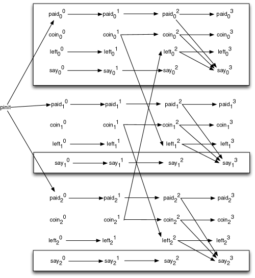
Figure 2: Timed-variable dependency graph after program unfolding

4 Valuation Algebra

Shenoy and Shafer [26, 28] have developed a general axiomatic formalism that captures the key properties that underpin the correctness of optimization methods used for a variety of uncertainty formalisms. In particular, it has been shown that this formalism allows for a general explanation of variable elimination algorithms and the notion of conditional independence used in the Bayesian Network literature [19], and applies also in other contexts such as Spohn’s theory of ordinal conditional functions [30]. There is a close connection also to ideas in database query optimization [22] and operations research [5]. We show here that Shenoy and Shafer’s general axiomatic framework applies to epistemic model checking. This will enable us to apply the variable elimination algorithm to derive techniques for optimizing epistemic model checking.

4.1 Axiomatic Framework

We begin by presenting Shenoy and Shafer’s framework, following [18]. Let $\mathit{Vars}$ be a set of variables, with each $v\in\mathit{Vars}$ taking values in a set $\Omega_{v}$. For a set $X$ of variables, the set $\Omega_{X}=\Pi_{x\in X}\Omega_{x}$ is called the frame of $X$. Elements of $\Omega_{X}$ are called configurations of $X$. In case $X=\emptyset$, the set $\Omega_{X}$ is interpreted as $\{\langle\rangle\}$, i.e., the set containing just the empty tuple. We write $D$ for ${\cal P}(\mathit{Vars})$.

A valuation algebra is a tuple $\langle\Phi,\mathit{dom},e,\otimes,\downarrow\rangle$, with components as follows. A state of information is represented in valuation algebra by a primitive notion called a valuation. Component $\Phi$ is a set, the set of all valuations, and $\mathit{dom}$ is function from $\Phi$ to ${\cal P}(\mathit{Vars})$. Intutitively, for each valuation $s\in\Phi$, the domain $\mathit{dom}(s)$ is the set of variables that the information is about. For a set of variables $X$, we write $\Phi_{X}$ for the set of valuations $s$ with $\mathit{dom}(s)=X$. Component $e$ gives an element $e_{X}\in\Phi_{X}$ for each $X\in D$. A valuation algebra also has two operations $\otimes:\Phi\times\Phi\rightarrow\Phi$ (combination) and $\downarrow:\Phi\times D\rightarrow\Phi$(marginalization), with $\otimes$, intuitively, representing the combination of two pieces of information, and $\downarrow$ used to restrict a piece of information to a given set of variables. Both are written as infix operators. From marginalization, another operator $-:\Phi\times\mathit{Vars}\rightarrow\Phi$ called variable elimination can be defined, by $s^{-x}=s\downarrow(\mathit{dom}(s)\setminus\{x\})$.

These operations are required to satisfy the following conditions:

1. Semigroup. $\otimes$ is associative and commutative. For all $X\in D$ and all $s\in\Phi_{X}$, we have $s\otimes e_{X}=e_{X}\otimes s=s$.

2. Domain of combination. For all $s,t\in\Phi$, $\mathit{dom}(s\otimes t)=\mathit{dom}(s)\cup\mathit{dom}(t)$.

3. Marginalization. For $s\in\Phi$ and $X,Y\in D$, the following hold:

   $$s\downarrow X=s\downarrow X\cap\mathit{dom}(s)\quad\quad\mathit{dom}(s\downarrow X)=X\cap\mathit{dom}(s)\quad\quad s\downarrow\mathit{dom}(s)=s~{}.$$

4. Transitivity of marginalization. For $s\in\Phi$, and $X\subseteq Y\subseteq\mathit{Vars}$,

   $$(s\downarrow Y)\downarrow X=s\downarrow X~{}.$$

5. Distributivity of marginalization over combination. For $s,t\in\Phi$, with $\mathit{dom}(s)=X$

   $$(s\otimes t)\downarrow X=s\otimes(t\downarrow X)~{}.$$

6. Neutrality. For $X,Y\in D$,

   $$e_{X}\otimes e_{Y}=e_{X\cup Y}~{}.$$

A key result that follows from these axioms, called the Fusion Algorithm [27], exploits Distributivity of Elimination over Combination to give a way of computing the result of a marginalization operation applied to a sequence of combinations, by pushing in variable eliminations over elements of the combination that do not contain the variable.

For a finite set $S=\{s_{1},s_{2},\ldots,s_{k}\}\subseteq\Phi$, write $\otimes S$ for $s_{1}\otimes s_{2}\otimes\ldots\otimes s_{k}$. We define the fusion of $S$ via $x\in\mathit{Vars}$ to be the set

$$\mathit{Fus}_{x}(S)=\{(\otimes S_{+})^{-x}\}\cup S_{-}~{}$$

where we have partitioned $S$ as $S_{+}\cup S_{-}$, such that $S_{+}$ is the set of $s\in S$ with $x\in\mathit{dom}(s)$, and $S_{-}$ is the set of $s\in S$ with $x\not\in\mathit{dom}(s)$. That is, in the fusion of the set $S$ with respect to $x$, we combine all the valuations with $x$ in their domain, and then eliminate $x$, and preserve all valuations with $x$ not in their domain.

Suppose we are interested in computing $(\otimes S)\downarrow X$, for $S$ a finite set of valuations, and $X\subseteq\mathit{Vars}$. The Fusion Algorithm achieves this by repeatedly applying the fusion operation, using some ordering of the variables in $X$. We write $\mathit{dom}(S)$ for $\mathit{dom}(\otimes S)=\bigcup\{\mathit{dom}(s)~{}|~{}s\in S\}$

Theorem 1 ([27]).

Let $S$ be a finite set of valuations, and $X\subseteq\mathit{Vars}$. Suppose $\mathit{dom}(S)\setminus X=\{x_{1},x_{2},\ldots,x_{n}\}$. Then

$$(\otimes S)\downarrow X=\otimes\mathit{Fus}_{x_{n}}(\ldots(\mathit{Fus}_{x_{1}}(S)))~{}.$$

Each ordering of the variables $x_{1}\ldots x_{n}$ gives a different way to compute $(\otimes S)\downarrow X$. A well chosen order can yield a significant optimization of the computation, by keeping the domains of the intermediate valuations in the sequence of fusions small. Finding an optimal order may be computationally complex, but there exist heuristics that produce good orders in practice [23, 20].

4.2 A Valuation Algebra of Relational Structures

We now show that the relational structures that underly Kripke structures are associated with algebraic operations that satisfy the conditions from the previous section. It will follow from this that the Fusion algorithm can be applied to these structures.

Let ${\cal V}$ be the set of all variables. Values in the algebra will be relational structures of the form $s=(A,V)$, where $V\subseteq{\cal V}$ and $A\subseteq\mathit{assgt}(V)$. The domain of a relational structure is defined to be its set of variables, i.e. if $s=(A,V)$ then $\mathit{dom}(s)=V$. We define the identities $e_{X}$ and operations $\otimes$ of combination and and $\downarrow$ of marginalization as follows. Let $s_{1}=(A_{1},V_{1})$ and $s_{2}=(A_{2},V_{2})$ and $X\subseteq{\cal V}$. Then

• $e_{X}=(\mathit{assgt}(X),X)$,

• $s_{1}\otimes s_{2}=(A,V)$ where $V=V_{1}\cup V_{2}$, and $A\subseteq\mathit{assgt}(V)$ is defined by $\alpha\in A$ iff $\alpha\upharpoonright V_{1}\in A_{1}$ and $\alpha\upharpoonright V_{2}\in A_{2}$.

• $s_{1}\downarrow X=(A,V)$ where $V=V_{1}\cap X$, and $A=\{\alpha\upharpoonright X~{}|~{}\alpha\in A_{1}\}$.

To use terminology from relational databases, $s_{1}\otimes s_{2}$ is the join of relations and $s\downarrow X$ is the projection of the relation $s$ onto attributes $X$. The following result is straightforward; these properties are well-known for relational algebra.

Proposition 3.

The algebra of relational structures satisfies axioms VA1-VA6.

We may extend the operation of marginalization in this valuation algebra to epistemic variable structures as follows. If $\mathcal{M}=(A,O,V)$ is an epistemic variable structure and $X\subseteq V$, we define $\mathcal{M}\downarrow X=(A^{\prime},O^{\prime},V^{\prime})$ where $A^{\prime}=\{\alpha\upharpoonright X~{}|~{}\alpha\in A\}$ and $O^{\prime}_{i}=O_{i}\cap X$ for all $i\in\mathit{Agts}$ and $V^{\prime}=V\cap X$. In general, this operation results in agents losing information, since their knowledge is based on the observation of fewer variables. Below, we identify conditions where knowledge is preserved by this operation.

5 Conditional Independence and Directed Graphs

5.1 Conditional Independence

Let $X,Y,Z\subseteq V$ be sets of variables. The notion of conditional independence expresses a generalized type of independency relation. Variables $X$ are said to be conditionally independent of $Y$, given $Z$, if, intuitively, once the values of $Z$ are known, the values of $Y$ are unrelated to the values of $X$, so that neither $X$ not $Y$ gives any information about the other. This intuition can be formalized for both both probabilistic and discrete models. The following definition gives a discrete interpretation, related to the notion of embedded multivalued dependencies from database theory [13].

Definition 1.

Let $A\subseteq\mathit{assgt}(V)$ be a set of assignments over variables $V$ and let $X,Y,Z\subseteq V$. We say that $A$ satisfies the conditional independency $X\bot Y|Z$, and write $A\models X\bot Y|Z$, if for every pair of worlds $u,v\in A$ with $u\upharpoonright Z=v\upharpoonright Z$, there exists $w\in A$ with $w\upharpoonright X\cup Z=u\upharpoonright X\cup Z$ and $w\upharpoonright Y\cup Z=v\upharpoonright Y\cup Z$. For an epistemic variable structure $\mathcal{M}=(A,O,V)$, we write $\mathcal{M}\models X\bot Y|Z$ if $A\models X\bot Y|Z$.

Conditional independencies can be deduced from graphical representations of models. Such representations have been used in the literature on Bayesian Nets [24, 19], and have also been applied in propositional reasoning [11, 12]. The following presentation is similar to [11] except that we work with relations over arbitrary domains rather than propositional formulas.

5.2 Directed Graphs

A directed graph is a tuple $G=(V,E)$ consisting of a set $V$ (the vertices) and a relation $E\subseteq V\times V$ (the edges). If $(u,v)\in E$ we say that there is an edge from $u$ to $v$, and may also denote this fact by $u\rightarrow v$. We write $u-v$ when both $u\rightarrow v$ and $v\rightarrow u$. The set of parents of a node $u$ is defined to be the set $\mathit{pa}(v)=\{u\in V~{}|~{}u\rightarrow v\}$. A path of length $n$ from $u$ to $v$ in $G$ is a sequence $u_{0},u_{1},\ldots,u_{n}$ of vertices, such that $u_{i}\rightarrow u_{i+1}$ for all $i=0\ldots n-1$. The graph is acyclic if there is no nontrivial path from any vertex to itself. We also call such a graph a directed acyclic graph, abbreviated as dag. An undirected graph is a graph with a symmetric edge relation $E$, i.e. if $u\rightarrow v$ then also $v\rightarrow u$. We may represent such a pair of edges with the notation $u-v$.

The notion of d-separation [24] provides a way to derive a set of independency statements from a directed graph $G$. We present here an equivalent formulation from [21], that uses the notion of the moralized graph $G^{m}$ of a directed graph $G$. The graph $G^{m}$ is defined to be the undirected graph obtained from $G$ by first adding an edge $u-v$ for each pair $u,v$ of vertices that have a common child (i.e. such that there exists $w$ with $u\rightarrow w$ and $v\rightarrow w$), and then replacing all directed edges with undirected edges. For a set of vertices $X$ of the directed graph $G$, we write $\mathit{An}(X)$ for the set of all vertices $v$ that are ancestors of some vertex $x$ in $S$ (i.e., such that there exists a directed path from $v$ to $x$). For a subset $X$ of the set of vertices of graph $G=(V,E)$, we defined the restriction of $G$ to $S$ to be the graph $G_{S}=(V\cap S,\{(u,v)\in E~{}|~{}u,v\in S\})$. For disjoint sets $X,Y,S$, we then have that $X$ is d-separated from $Y$ by $S$ if all paths from $X$ to $Y$ in $(G_{\mathit{An}(X\cup Y\cup S)})^{m}$ include a vertex in $S$.

A structured model for a valuation algebra $\langle\Phi,\mathit{dom},e,\otimes,\downarrow\rangle$, is a tuple $M=\langle V,E,{\cal S}\rangle$ where $V$ is a set of variables, $D={\cal P}(V)$, component $E$ is a binary relation on $V$ such that $G_{M}=(V,E)$ is a dag, and ${\cal S}=\{s_{v}\}_{v\in V}$ is a collection of values in $\Phi$ such that for each variable $v\in V$, we have

• $\mathit{dom}(s_{v})=\{v\}\cup\mathit{pa}(v)$, i.e. the domain of $s_{v}$ consists of $v$ and its parents in the dag,

• $s_{v}\downarrow{\mathit{pa}(v)}=e_{\mathit{pa}(v)}$.

Intuitively, the second constraint says that the relation $s_{v}$ does not constrain the parents of $v$: for each assignment of values to the parents of $v$, there is at least one value of $v$ that is consistent.

The following is a consequence of results in [24, 21, 33].

Proposition 4.

Suppose that $M=\langle V,E,{\cal S}\rangle$ is a structured model and $X,Y,Z$ are disjoint subsets of the vertices $V$ of the directed graph $G=(V,E)$. If $X$ is d-separated from $Y$ by $Z$, then $\otimes{\cal S}\models X\bot Y|Z$.

Proof.

(Sketch) The set $I$ of conditional independency statements holding in a structured model is a semi-graphoid. In particular, we will take $I$ to be the semi-graphoid of conditional independencies in $\otimes{\cal S}$.

A stratified protocol $L$ of $I$ is an ordering $v_{1}\ldots v_{n}$ of $V$ together with a function $p:V\rightarrow{\cal P}(V)$ such that for all $i=1\ldots n$, we have that $p(v_{i})\subseteq\{v_{1},\ldots,v_{i-1}\}$ and the set $I$ contains the statement

$$\{v_{1}\ldots v_{i-1}\}\setminus p(v_{i})\bot\{v_{i}\}|p(v_{i})~{}.$$

Each stratified protocol $L$ is associated with a directed acyclic graph $dag(L)=(V,\{(u,v)~{}|~{}v\in V,~{}u\in p(v)\})$. It follows from the fact that $M$ is a structured relational model that any topological sort of $G$, together with the parent function in $G$ as the function $p$, is a stratified protocol $L$ of $I$, and we have $dag(L)=G$.

Verma and Pearl [33](Theorem 2) show that if $Z$ d-separates $X$ from $Y$ in $dag(L)$ and $L$ is a stratified protocol for a semi-graphoid $I$, then $X\bot Y|Z$ is in $I$. It follows that if $Z$ d-separates $X$ from $Y$ in $G$ then $\otimes{\cal S}\models X\bot Y|Z$. ∎

Structured models have an additional property that provides an optimization when eliminating variables: if a leaf node is one of the variables eliminated from the combination of the nodes of the graph, then it can be simply removed from the model without changing the result. This is formally captured in the following result.

Proposition 5.

Suppose that $M=\langle V,E,{\cal S}\rangle$ is a structured model, let $X\subseteq V$ and let $v\in V\setminus X$ be a leaf node. Then $\otimes{\cal S}\downarrow X=\otimes({\cal S}\setminus\{s_{v}\})\downarrow X$.

Proof.

Let $s=\otimes({\cal S}\setminus\{s_{v}\})$. By the semigroup properties, we have $\otimes{\cal S}=s\otimes s_{v}$. We first note that

$$(s\otimes s_{v})\downarrow\mathit{dom}(s) =s\otimes(s_{v}\downarrow\mathit{dom}(s))$$ by VA5

$$=s\otimes(s_{v}\downarrow\mathit{dom}(s)\cap\mathit{dom}(s_{v}))$$ by VA3

$$=s\otimes(s_{v}\downarrow\mathit{pa}(v)) v$$ since is a leaf

$$=s\otimes e_{v} M$$ since is a s.r.m.

$$=s$$ by VA1.

Hence

$$(s\otimes s_{v})\downarrow X =(s\otimes s_{v})\downarrow\mathit{dom}(s)\cap X X\subseteq\mathit{dom}(s)$$ since

$$=(s\otimes s_{v})\downarrow\mathit{dom}(s)\downarrow X$$ by VA4

$$=s\downarrow X$$ by the result above.

∎

To apply these results for structured models to model checking epistemic logic, we use the following definition. We say that a structured model $M=\langle V,E,{\cal S}\rangle$ represents the worlds of an epistemic variable structure $\mathcal{M}=(A,O,U)$ if $V=U$ and $A=\otimes{\cal S}$. That is, the structured model captures the set of assignments making up the epistemic variable structure.

5.3 Eliminating Observable Variables

Consider the following formulation of the model checking problem: for an epistemic formula $\phi$, we wish to verify $\mathcal{M}\models\phi$ where $\mathcal{M}=(A,O,V)$ is an epistemic variable structure with observable variables $O$, with worlds represented by a structured model $M=\langle V,E,{\cal S}\rangle$.

A first idea for how to optimize this verification problem is to reduce the structure $\mathcal{M}$ to the set of variables $\mathit{vars}(\phi)$ of the formula $\phi$, on the intuition that only these variables are relevant to the satisfaction of $\phi$. But this is not quite correct: the formula may contain the epistemic operators $K_{i}$, the semantics of which refers to the observable variables $O_{i}$, since these are used to define the indistinguishability relation. Thus a more accurate claim is that we should restrict the structure to $\mathit{vars}(\phi)$, together with the sets $O_{i}$ for any operator $K_{i}$ in $\phi$.

In fact, using the notion of conditional dependence, it is often possible to identify a smaller set of variables that suffices to verify the formula. The intuition for this is that some of the observed variables in $O_{i}$ may be independent of the variables in the formula, and moreover, information may be redundantly encoded in the observable variables. For example, if an observable variable that does not itself occur in the formula is computed from other observable variables, then it is redundant from the point of view of determining the possible values of variables in the formula. The following definitions strengthen the idea of restricting to $\mathit{vars}(\phi)\cup O$ by exploiting a sufficient condition for the removal of observable variables.

Say that $\kappa$ is a relevance function for a formula $\phi$ with respect to an epistemic variable structure $\mathcal{M}=(A,O,V)$ if it maps subformulas of $\phi$ to subsets of the set of variables $V$, and satisfies the following conditions:

1. $\kappa(p)=\{p\}$ for $p\in V$,

2. $\kappa(\phi_{1}\land\phi_{2})=\kappa(\phi_{1})\cup\kappa(\phi_{2})$,

3. $\kappa(\neg\phi_{1})=\kappa(\phi_{1})$, and

4. $\kappa(K_{i}\phi_{1})=U_{i}\cup\kappa(\phi_{1})$, for some $U_{i}\subseteq O_{i}$ with $\kappa(\phi_{1})\cap O_{i}\subseteq U_{i}$ and $\mathcal{M}\models(\kappa(\phi_{1})\setminus U_{i})\bot(O_{i}\setminus U_{i})|U_{i}$.

In the final condition, $U_{i}$ can be any set. We note that a set $U_{i}$ satisfying the condition can always be found. For, if we take $U_{i}=O_{i}$, then the condition states that $\kappa(\phi_{1})\cap O_{i}\subseteq O_{i}$ and $M\models(\kappa(\phi_{1})\setminus O_{i})\bot\emptyset|O_{i}$. Both parts of this statement are trivially true. In practice, we will want to choose $U_{i}$ to be as small as possible, since this will lead to stronger optimizations.

Note that $\phi$ is a subformula of itself, so in the domain of $\kappa$. The following result says that satisfaction of $\phi$ is preserved when we marginalize to a superset of $\kappa(\phi)$ for a relevance function $\kappa$.

Theorem 2.

Suppose that $\kappa$ is a relevance function for $\phi$ with respect to epistemic variable structure $\mathcal{M}$ and that $X$ is a set of variables with $\kappa(\phi)\subseteq X\subseteq\mathit{dom}(\mathcal{M})$. Then for all worlds $w$ of $\mathcal{M}$, we have $\mathcal{M},w\models\phi$ iff $\mathcal{M}\downarrow X,w\upharpoonright X\models\phi$.

Proof.

We prove the result, for all epistemic variable structures $\mathcal{M}$, by induction on the structure of $\phi$. Suppose $\kappa(\phi)\subseteq X\subseteq\mathit{dom}(\mathcal{M})$.

For the case $\phi=p\in V$, we have $\kappa(\phi)=\{p\}$, so $p\in X$. Hence $\mathcal{M},w\models\phi$ iff $w(p)=1$ iff $(w\upharpoonright X)(p)=1$ iff $\mathcal{M}\downarrow X,w\upharpoonright X\models\phi$, as required.

In case $\phi=\phi_{1}\land\phi_{2}$, we have $\kappa(\phi)=\kappa(\phi_{1})\cup\kappa(\phi_{2})$, so $\kappa(\phi_{1})\subseteq X$ and $\kappa(\phi_{2})\subseteq X$. Hence

$$\mathcal{M},w\models\phi \text{ iff }\mathcal{M},w\models\phi_{1}\text{ and }\mathcal{M},w\models\phi_{2}$$

$$\text{ iff }\mathcal{M}\downarrow X,w\upharpoonright X\models\phi_{1}\text{ and }\mathcal{M}\downarrow X,w\upharpoonright X\models\phi_{2}$$ (by induction)

$$\text{ iff }\mathcal{M}\downarrow X,w\upharpoonright X\models\phi~{}.$$

The proof for the case $\phi=\neg\phi_{1}$ is similar.

In case $\phi=K_{i}\phi_{1}$, we show that $\mathcal{M},w\models K_{i}\phi_{1}$ implies $\mathcal{M}\downarrow X,w\upharpoonright X\models K_{i}\phi_{1}$, and the converse. Note that the equivalence relation $\sim^{\prime}_{i}$ used in the semantics of the operator $K_{i}$ in $\mathcal{M}\downarrow X$ is given by $v\sim^{\prime}_{i}w$ if $v\upharpoonright O_{i}\cap X=w\upharpoonright O_{i}\cap X$.

For the implication from $\mathcal{M},w\models K_{i}\phi_{1}$ to $\mathcal{M}\downarrow X,w\upharpoonright X\models K_{i}\phi_{1}$, suppose that $\mathcal{M},w\models K_{i}\phi_{1}$. Let $w\upharpoonright X\sim^{\prime}_{i}v$, where $v$ is a world of $\mathcal{M}\downarrow X$. Then there exists a world $u$ of $\mathcal{M}$ such that $u\upharpoonright X=v$. We need to show that $\mathcal{M}\downarrow X,u\upharpoonright X\models\phi_{1}$. Since $U_{i}\subseteq\kappa(K_{i}\phi_{1})\subseteq X$ and $U_{i}\subseteq O_{i}$, we have $U_{i}\subseteq X\cap O_{i}$. Hence, from $w\upharpoonright X\sim^{\prime}_{i}u\upharpoonright X$, we have $w\upharpoonright U_{i}=u\upharpoonright U_{i}$. Thus, from $M\models(\kappa(\phi_{1})\setminus U_{i})\bot(O_{i}\setminus U_{i})|U_{i}$, it follows that there exists a world $w^{\prime}$ of $\mathcal{M}$ such that $w^{\prime}\upharpoonright(O_{i}\setminus U_{i})\cup U_{i}=w\upharpoonright(O_{i}\setminus U_{i})\cup U_{i}$ and $w^{\prime}\upharpoonright(\kappa(\phi_{1})\setminus U_{i})\cup U_{i}=u\upharpoonright(\kappa(\phi_{1})\setminus U_{i})\cup U_{i}$. Thus, $w^{\prime}\upharpoonright O_{i}=w\upharpoonright O_{i}$ and $w^{\prime}\upharpoonright\kappa(\phi_{1})=u\upharpoonright\kappa(\phi_{1})$. Hence

$$\mathcal{M},w^{\prime}\models\phi_{1}~{}~{}~{}~{} \text{iff }\mathcal{M}\downarrow\kappa(\phi_{1}),w^{\prime}\upharpoonright\kappa(\phi_{1})\models\phi_{1}$$ (by induction)

$$\text{iff }\mathcal{M}\downarrow\kappa(\phi),u\upharpoonright\kappa(\phi)\models\phi_{1} w^{\prime}\upharpoonright\kappa(\phi_{1})=u\upharpoonright\kappa(\phi_{1})$$ (by )

$$\text{iff }\mathcal{M},u\models\phi_{1}$$ (by induction)

Since $w^{\prime}\upharpoonright O_{i}=w\upharpoonright O_{i}$ and $\mathcal{M},w\models K_{i}\phi_{1}$, we have $\mathcal{M},w^{\prime}\models\phi_{1}$. Hence $\mathcal{M},u\models\phi_{1}$. By induction, $\mathcal{M}\downarrow X,u\upharpoonright X\models\phi_{1}$, as required.

Conversely, suppose that $\mathcal{M}\downarrow X,w\upharpoonright X\models K_{i}\phi_{1}$. We show that $\mathcal{M},w\models K_{i}\phi_{1}$. For this, let $u$ be a world of $\mathcal{M}$ with $w\upharpoonright O_{i}=u\upharpoonright O_{i}$. We need to show that $\mathcal{M},u\models\phi_{1}$. For this, note that it follows from $w\upharpoonright O_{i}=u\upharpoonright O_{i}$ that $w\upharpoonright X\upharpoonright O_{i}\cap X=u\upharpoonright X\upharpoonright O_{i}\cap X$, i.e., $w\upharpoonright X\sim^{\prime}_{i}u\upharpoonright X$. Since $\mathcal{M}\downarrow X,w\upharpoonright X\models K_{i}\phi_{1}$, we have that $\mathcal{M}\downarrow X,u\upharpoonright X\models\phi_{1}$. Since $\kappa(\phi_{1})\subseteq X$, we have, by induction, that $\mathcal{M},u\models\phi_{1}$, as required. ∎

Computing $\kappa(\phi)$: The definition of $\kappa$ provides a recursive definition by which $\kappa(\phi)$ can be calculated, with the exception that the case $\kappa(K_{i}(\phi))=U_{i}\cup\kappa(\phi)$ allows for a choice of the set $U_{i}$, subject to the conditions $\kappa(\phi)\cap O_{i}\subseteq U_{i}$ and $\mathcal{M}\models(\kappa(\phi)\setminus U_{i})\bot(O_{i}\setminus U_{i})|U_{i}$. When the worlds of $\mathcal{M}$ are represented by a structured relational model $M$, we show how to construct the minimal set $U_{i}$ satisfying the stronger conditions that $\kappa(\phi)\cap O_{i}\subseteq U_{i}$ and $U_{i}$ d-separates $\kappa(\phi)\setminus U_{i}$ from $O_{i}\setminus U_{i}$ in the directed graph $G$ associated with $M$.

Note $(\kappa(\phi)\setminus U_{i})\cup(O_{i}\setminus U_{i})\cup U_{i}=\kappa(\phi)\cup O_{i}$ for any set $U_{i}$. Thus, the d-separation properties we are interested in are computed in the moralized graph $H=(G_{\mathit{An}(O_{i}\cup\kappa(\phi))})^{m}$, which is independent of $U_{i}$. Let $U$ be the set of vertices $v\in O_{i}$ such that there exists a path in $H$ from a vertex $u\in\kappa(\phi)\setminus O_{i}$ to $v$, with $v$ the first vertex on that path that is in $O_{i}$. The set $U$ can be constructed in linear time by a depth first search from $\kappa(\phi)\setminus O_{i}$. Take $W=U\cup(\kappa(\phi)\cap O_{i})$.

Proposition 6.

$W$ is the smallest set satisfying the strengthened conditions for $U_{i}$.

Proof.

We first show that $W$ satisfies the conditions for $U_{i}$. Clearly $\kappa(\phi)\cap O_{i}\subseteq W$. We show that $\kappa(\phi)\setminus W$ is d-separated from $O_{i}\setminus W$ by $W$. Let $u=u_{0},u_{1},\ldots,u_{n}=v$ be a path in $H$ from $u\in\kappa(\phi)\setminus W$ to $O_{i}\setminus W$. Since $\kappa(\phi)\cap O_{i}\subseteq W$, we have $u\not\in O_{i}$. But then the path must cross an edge from the exterior of $O_{i}$ into $O_{i}$, and the endpoint of that edge is in $W$, by definition. This shows that there is no path from $\kappa(\phi)\setminus W$ to $O_{i}\setminus W$ that avoids $W$. Thus, $W$ satisfies the conditions for $U_{i}$.

To show that $W$ is the minimal such set, let $U_{i}$ be any set satisfying the conditions, and suppose that $W\not\subseteq U_{i}$. Then there is a vertex $v\in W\setminus U_{i}$. Since $W\subseteq O_{i}$, we have $v\in O_{i}\setminus U_{i}$. We cannot have $v\in\kappa(\phi)\cap O_{i}$, since then also $v\in U_{i}$. Thus, by definition of $W$, there exists a path in $H$ from $v$ to some node in $\kappa(\phi)\setminus O_{i}$, with all vertices after $v$ not in $O_{i}$, hence also not in $U_{i}$ since $U_{i}\subseteq O_{i}$. Note $\kappa(\phi)\setminus O_{i}=\kappa(\phi)\setminus U_{i}$ since $\kappa(\phi)\cap O_{i}\subseteq U_{i}$. Thus, $\kappa(\phi)\cap O_{i}\subseteq U_{i}$ is not d-separated from $O_{i}\setminus U_{i}$ by $U_{i}$, contradicting the assumptions on $U_{i}$. This shows that $W\subseteq U_{i}$. ∎

5.4 Equalities

Unfolding a program into a structured model tends to create a large number of timed variable instances whose associated value represents an equality between two variables. Such instances can be eliminated by a simple transformation of the structured model.

For an assignment $\alpha$ with domain $V$, define $\alpha[y/x]$ to be the assignment $\alpha^{\prime}$ with domain $(V\setminus\{x\})\cup\{y\}$ with $\alpha(y)=\alpha^{\prime}(x)$ and $\alpha\upharpoonright(\mathit{dom}(s)\setminus\{x\})=\alpha^{\prime}\upharpoonright(\mathit{dom}(s)\setminus\{x\})$.

For a relational value $s$ and variables $x,y$ with $x\in\mathit{dom}(s)$ and $y\not\in\mathit{dom}(s)$, define $s[y/x]$ to be the relational value $t$ with $\mathit{dom}(t)=(\mathit{dom}(s)\setminus\{x\})\cup\{y\}$, consisting of all assignments $\alpha[y/x]$ for $\alpha\in s$. Intuitively, this is simply the relation $s$ with variable $x$ renamed to $y$.

We extend this definition to structured relational models $M=(V,E,{\cal S})$ with $x,y\in V$, by defining $M[y/x]=(V^{\prime},E^{\prime},{\cal S}^{\prime})$ with $V^{\prime}=V\setminus\{x\}$, and $E^{\prime}=E\cap(V^{\prime}\times V^{\prime})$, and ${\cal S}=\{s^{\prime}_{v}~{}|~{}v\in V^{\prime}\}$, where $s^{\prime}_{v}=s[y/x]$. In the following result, we write $\delta_{x,y}$ for the set of assignments $\alpha$ with domain $\{x,y\}$ and $\alpha(x)=\alpha(y)$.

Proposition 7.

Suppose that $M=(V,E,{\cal S})$ is a structured relational model with $x,y\in V$, and $\Omega_{x}=\Omega_{y}$, and $\mathit{pa}(y)=\{x\}$ and $s_{y}=\delta_{x,y}$. Let $M[y/x]=(V^{\prime},E^{\prime},{\cal S}^{\prime})$. Then $\otimes{\cal S}^{\prime}=(\otimes{\cal S})\downarrow V^{\prime}$.

The definition furthermore extends to epistemic models $\mathcal{M}=(A,O,V)$ with worlds represented by a structured relational model $M=(V,E,{\cal S})$. Let $M[y/x]=(V^{\prime},E^{\prime},{\cal S}^{\prime})$. We define $\mathcal{M}[x/y]=(A^{\prime},O^{\prime},V^{\prime})$ where $O^{\prime}=\{O^{\prime}_{i}\}_{i\in\mathit{Agts}}$ where $O^{\prime}_{i}=O_{i}\cup\{y~{}|~{}x\in O_{i}\}$ for each $i\in\mathit{Agts}$, and $A^{\prime}=\otimes{\cal S}^{\prime}$. Note that $O^{\prime}_{i}$ additionally makes variable $y$ visible to agent $i$ if $x$ was visible to $i$, in case this variable was not originally visible.

Proposition 8.

If $\Omega_{x}=\Omega_{y}$, and $\mathit{pa}(y)=\{x\}$ and $s_{y}=\{(x:a,y:a)~{}|~{}a\in\Omega_{x}\}$ then $\mathcal{M},\alpha\models\phi$ iff $\mathcal{M}[y/x],\alpha[y/x]\models\phi[y/x]$.

5.5 Algorithm

The overall optimized procedure for model checking that we obtain from the above results uses the following steps:

1. We first unfold a program representation of the model into a structured relational model with symbolically represented values and transform the query into a form that uses the timed instances variables in place of the original variables. This can be done in a way that builds in the equality optimization of Section 5.4. We expand on this step in Section 7.

2. We compute $\kappa(\phi)$ using the algorithm in Section 5.3.

3. We compute a symbolic representation of $\mathcal{M}\upharpoonright\kappa(\phi)$, using the leaf node elimination optimization.

4. We compute $\mathcal{M}\upharpoonright\kappa(\phi)\models\phi$ in this representation using a symbolic model checking algorithm.

6 Example

In the present section, we illustrate this procedure on the Dining cryptographers protocol.

Figure 5 indicates the dependency graph that remains after we have applied the optimization procedure to the Dining cryptographers problem. We consider the formula

$$\phi=(\neg\mathit{paid}_{0}\Rightarrow K_{0}(\neg\mathit{paid}_{1}\land\neg\mathit{paid}_{2})\lor(K_{0}(\mathit{paid}_{1}\lor\mathit{paid}_{1})\land\neg K_{0}\mathit{paid}_{1}\land\neg K_{0}\mathit{paid}_{2})$$

evaluated at time 3. Transforming to timed form, this is

$$\phi_{1}=(\neg\mathit{paid}^{3}_{0}\Rightarrow K_{0}(\neg\mathit{paid}^{3}_{1}\land\neg\mathit{paid}^{3}_{2})\lor(K_{0}(\mathit{paid}^{3}_{1}\lor\mathit{paid}^{3}_{1})\land\neg K_{0}\mathit{paid}^{3}_{1}\land\neg K_{0}\mathit{paid}^{3}_{2})$$

The set of observable variables $O_{0}$ used for the operator $K_{0}$ in this formula is the set of all variables inside the rectangles in Figure 2.

The result of applying the equality optimization to the model is depicted in Figure 3. The resulting formula is

$$\phi_{2}=(\neg\mathit{paid}^{0}_{0}\Rightarrow K_{0}(\neg\mathit{paid}^{0}_{1}\land\neg\mathit{paid}^{0}_{2})\lor(K_{0}(\mathit{paid}^{0}_{1}\lor\mathit{paid}^{0}_{1})\land\neg K_{0}\mathit{paid}^{0}_{1}\land\neg K_{0}\mathit{paid}^{0}_{2})$$

Figure 3: Depency graph after equality optimization

To construct the moralized graph, we add edges between all vertices in the sets $\{\mathit{paid}^{2}_{i},\mathit{coin}^{2}_{i},\mathit{left}^{2}_{i}\}$ for $i=0,1,2$, and replace all directed edges with undirected edges. The result is depicted in Figure 4.

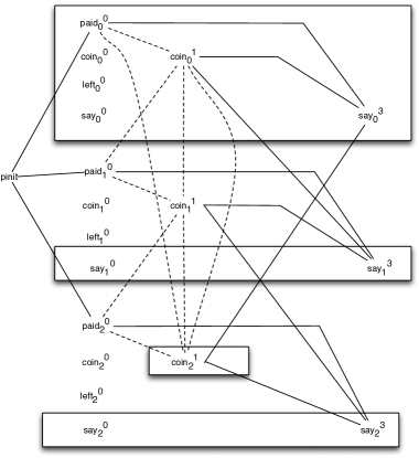
Figure 4: Moralised graph

For the computation of $\kappa{\phi}$, we note that the variables in the scope of the knowledge operator are $\mathit{paid}_{1}^{0}$ and $\mathit{paid}_{2}^{0}$. The vertices at the outer boundary to the observable variables from these vertices are $\mathit{pinit},\mathit{paid}_{1}^{0},\mathit{paid}_{2}^{0},\mathit{coin}^{1}_{1}$. The observable variables reachable in one step from this outer boundary are $\mathit{paid}_{0}^{0},\mathit{coin}^{1}_{0},\mathit{coin}^{1}_{1},\mathit{say}^{3}_{1},\mathit{say}^{3}_{2}$. Thus, we compute

$$\kappa(\phi_{2})=\{\mathit{paid}_{0}^{0},\mathit{paid}_{1}^{0},\mathit{paid}_{2}^{0}\mathit{coin}^{1}_{0},\mathit{coin}^{1}_{1},\mathit{say}^{3}_{1},\mathit{say}^{3}_{2}\}$$

All other variables can be eliminated using the variable elimination algorithm. As a first step in this process, we can delete leaf nodes not in $\kappa(\phi_{2})$ (and recursively, any fresh leaf nodes not in $\kappa(\phi_{2})$ resulting from such deletions.) This step enables deletion of variables $\mathit{say}^{3}_{0}$ and $\mathit{coin}_{i}^{0},\mathit{left}^{0}_{i},say^{0}_{i}$ for $i=0,1,2$. The graph resulting from these deletions in depicted in Figure 5.

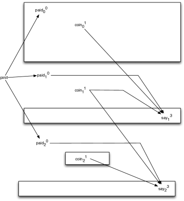
Figure 5: Dining Cryptographers Dependency graph after optimization

From the point of model checking complexity, we expect that the simplification of the dependency graph will result in significant improved performance of the model checking computation. For $n$ cryptographers, the initial dependency graph (Figure 2 for $n=3$) has $16n$ variables, i.e., $48$ variables in case $n=3$. The algorithm of van der Meyden and Su [31] would construct a BDD with over $12+4n$ variables in general, and, as show in Figure 6, with 24 variables in case $n=3$. However, the algorithm uses an intermediate BDD representation of the transition relation of the protocol that requires $8n$ variables. Instead, the optimization approach developed here computes a BDD over just 9 variables in case $n=3$ and $3n$ variables in general. The actual model checking computation combines BDD’s associated with each node to construct a BDD over the same number of variables. Since in practice, BDD algorithms work for numbers of variables in the order of 100-200, these reductions of the constant factor can have a significant impact on the scale of the problems that can be solved.

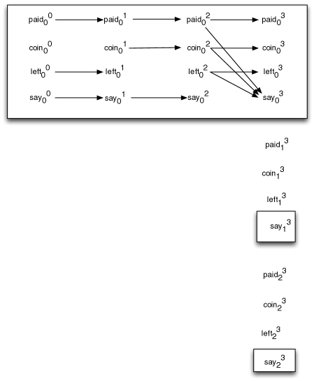
Figure 6: Timed-variables used in algorithm of van der Meyden and Su.

7 From Programs to Dags

We have developed an implementation of the above ideas as an extension of the epistemic model checker MCK [14]. We sketch the implementation in this section.

We apply the conditional independence optimization described above on a structured model derived from the system, in which values are represented symbolically as formulas. Given a formula to be model checked, we derive a structured model over a smaller set of vertices using the conditional independence optimization. Rather than producing the timed variable dag as in the discussion of the Dining Cryptographers example above, and then applying the equational optimization, the initial structured model is obtained by means of a symbolic execution that builds in the equational optimization. This symbolic execution proceeds as follows.

For a set of variables $\mathit{Vars}$, define an indexing of $\mathit{Vars}$ to be a mapping $\gamma:\mathit{Vars}\rightarrow\bf N$. If $\gamma$ is an indexing, and $e$ is an expression, we define the the expression $e/\gamma$, which interprets $e$ with respect to indexed instances of the variables, by replacing each occurrence of a variable $v$ in $e$ by the indexed variable $v^{\gamma(v)}$. Intuitively, $v^{k}$ represents the $k$-th value taken on by variable $v$ during the running of the program. (Note that this differs from the timed variable $v_{k}$, which represents the value of the variable at time $k$.)

Consider a system ${\cal I}=(J,I,Q)$ with joint protocol $J=P_{1}~{}||~{}\ldots~{}||~{}P_{n}~{}\Delta~{}C_{E}$. We can, for each time $t$ up to the maximal running time $N$ of $J$, obtain the code at time $t$, denoted $C_{t}=C^{t}_{1};\ldots C^{t}_{n};C_{E}$, where the $t$-th atomic statement in each $P_{i}$ is $\langle C^{t}_{i}\rangle$. (At this step, we use the fact that the agent protocols are straightline.) We construct a sequence of structured models $M_{0},\ldots,M_{N}$, and a sequence of indexings $\gamma_{0},\ldots\gamma_{N}$ of $\mathit{Vars}$, as follows.

To represent the initialization condition, we use a variable $v_{init}$ with frame $\Omega_{v_{init}}$ equal to the set of assignments over $vars(I)$. (Under our simplifying assumptions, this is a set of assignments to boolean variables; all indexed variables other than $v_{init}$ are boolean.)

The initial structured model $M_{0}=\langle V_{0},E_{0},{\cal S}\rangle$ has $V_{0}=\{v^{0}~{}|~{}v\in\mathit{Vars}\}\cup\{v_{init}\}$ and $E_{0}=\{(v_{init},v^{0})~{}|~{}v\in vars(I)\}$. Write $s_{u}=(A_{u},V_{u})$ for the values ${\cal S}=\{s_{u}\}_{u\in V_{0}}$. The domains of these values are given by $V_{v_{init}}=\{v_{init}\}$ and $V_{v^{0}}=\{v^{0}\}$ if $v\not\in vars(I)$ and $V_{v^{0}}=\{v_{init},v^{0}\}$ otherwise. The relations in these values are symbolically represented $A_{v_{init}}=I$, and $A_{v^{0}}=True$ if $v\not\in vars(I)$, otherwise by $v^{0}=v$. The indexing $\gamma_{0}$ is the initial indexing, which has $\gamma_{0}(v)=0$ for all $v\in\mathit{Vars}$.

Given model $M_{i}$, indexing $\gamma_{i}$ and code $C_{i}$, we obtain the next model and indexing in the sequence as $(M_{i+1},\gamma_{i+1})=\mu(M_{i},\gamma_{i},C_{i})$, where the function $\mu$ is defined by

$$\mu(M,\gamma,\epsilon)=(M,\gamma)$$

and

$$\mu(\langle V,E,{\cal S}\rangle,\gamma,(b;C))=(\langle V^{\prime},E^{\prime},{\cal S}^{\prime}\rangle,\gamma^{\prime},C)$$

where, if $b$ is the assignment $v:=e$ we have

$$\begin{array}[]{l}V^{\prime}=V\cup\{v_{\gamma(v)+1}\}\\ E^{\prime}=E\cup\{(u_{\gamma(u)},v_{\gamma(v)+1})~{}|~{}u\in vars(e)\}\\ {\cal S}^{\prime}={\cal S}\cup\{s_{v_{\gamma(v)+1}}\}\\ \gamma^{\prime}=\gamma[\gamma(v)+1/v]\end{array}$$

with the relation of $s_{v_{\gamma(v)+1}}$ symbolically represented by the formula $v_{\gamma(v)+1}\Leftrightarrow e/\gamma$. That is, the function $\mu$ processes an assignment statement $v:=e$ by interpreting $e$ with respect to $\gamma$, creating a new vertex $v_{\gamma(v)+1}$ with parents the variables in this interpretation $e/\gamma$ and a value that describes how $v_{\gamma(v)+1}$ is calculated from its parents.

In case $b$ is the randomization statement $rand(v)$, we take

$$\begin{array}[]{l}V^{\prime}=V\cup\{v_{\gamma(v)+1}\}\\ E^{\prime}=E\\ {\cal S}^{\prime}={\cal S}\cup\{s_{v_{\gamma(v)+1}}\}\\ \gamma^{\prime}=\gamma[\gamma(v)+1/v]\end{array}$$

with the relation of $s_{v_{\gamma(v)+1}}$ symbolically represented by the formula $True$.

The sequence of indexings $\gamma_{0}\ldots v_{N}$ relates timed variables to indexed variables, by the mapping $v_{t}\mapsto\gamma_{t}(v)$. Via this mapping, the structured model $M_{N}$ represents the worlds of the epistemic variable structure $\mathcal{M}_{N}({\cal I})$.

In particular, to evaluate an epistemic formula $\phi$ at time $N$, we work with the model $M_{N}$ and interpret each variable $v$ of $\phi$ as the indexed variable $\gamma_{N}(v)$. In order to determine $\kappa(\phi)$, where $\phi$ is a formula to be evaluated at time $N$, we use the sets $O_{i}=\{v^{t}~{}|~{}v\in Q_{i},~{}0\leq t\leq\gamma_{N}(v)\}$ of images of observable timed variables.

After constructing the structured model $M_{N}$ and computing the set of relevant variables $\kappa(\phi)$, we compute $M_{N}\upharpoonright\kappa(\phi)$ using the leaf node optimization. This is again a structured model. Since the values in $M_{N}$ are formulas, $M_{N}\upharpoonright\kappa(\phi)$ is represented as a formula of quantified boolean logic. We then process this formula from the leaves to the root to obtain a binary decision diagram representing this QBF formula – the variables in this representation are the variables in $\kappa(\phi)$. The assignments represented by this binary decision diagram are the worlds of a Kripke structure.

The observable variables yield binary relations over these worlds, defined by $w\sim_{i}w^{\prime}$ if for all variables $v\in O_{i}$, we have $w(v^{\gamma_{N}(v)})=w^{\prime}(v^{\gamma_{N}(v)})$. These relations correspond to an agent with perfect perfect recall observing variables $O_{i}$. The relations can similarly be represented by binary decision diagrams. This yields a symbolic representation of the Kripke structure using binary decision diagrams.

A standard symbolic evaluation procedure for modal logic can then be used to compute a BDD representing the set of worlds where $\neg\phi$ holds. We check this for emptiness to decide $M\models\phi$.

8 Experimental Results

In the present section, we describe the results of a number of experiments designed to evaluate the performance of epistemic model checking using the conditional independence optimization, in comparison with the existing implementation in MCK. (Since MCK remains the only symbolic epistemic model checker that deals with perfect recall knowledge, there are no other systems to compare to.) All experiments were conducted on an Intel 2.8 GHz Intel Core i5 processor with 8 GB 1600 MHz DDR3 memory running Mac OSX 10.10.

The experiments conducted are based on a number of examples of epistemic model checking applications that have previously been considered in the literature. Most concern security protocols. Each experiment scales according to a single numerical parameter, and we measure the running time of model checking a formula as a function of this parameter. Details of the protocols and the way that they are represented in the MCK scripting language when using the conditional independence optimization are presented in Appendix A.

The performance of the conditional independence optimization depends on the extent to which it is able to reduce the number of variables that need to be handled in the ultimate BDD calculation that implements model checking. Theoretically, in the worst case, there is no reduction in the number of variables. We have therefore deliberately chosen some examples in which the reduction is realised in order to demonstrate its power when it applies. However, the examples are realistic in that they derive from prior, independently motivated work.

Except where indicated, the unoptimized model checking algorithm against which we compare is that invoked by the construct spec_spr_xn in the MCK scripting language, which operates as already described above. (We refer to this algorithm as xn in legends, and the algorithm using conditional independence optimization is referenced as ci.) The results demonstrate both significant speedups of as large as four orders of magnitude, as well as a significant increase in the scale of problem that can be handled in a give amount of time.

Due to nondeterminism in the underlying CUDD package [29] used by MCK for binary decision diagram computations, the running times can show significant variance from run to run, with some runs taking very large amounts of time. We have dealt with this variance by concentrating on the minimal running time obtained over three runs of the experiments. This form of aggregation can be justified as equivalent to the running time obtained when running three copies of the computation in parallel and taking the answer from the first to complete.

Even with this allowance, the plot of running times as we scale the experiments can be very jagged on larger instances. The problem tends to affect the unoptimized running times more than the running times using the conditional independence optimization, which generally give smooth curves. We believe this is due to memory placement effects on larger BDD’s, and because the BDD’s for the unoptimized running times reach the critical size significantly earlier. We expect that a similar phenomenom will occur with the optimized version once this critical BDD size is reached.

8.1 Dining Cryptographers

Our first example is the Dining Cryptographers protocol [10], as discussed in Section 3. This scales by the number $n$ of agents; the number of state variables is $O(n)$, and the protocol runs for 3 steps. The initial condition needs to say that at most one of the agents paid – this is done by means of a formula of size $O(n^{2})$. The rest of the script scales linearly. The formula in all instances states that at time 3, agent $C0$ either knows that no agent pays, knows that C0 is the payer, or knows that one of the other cryptographers is the payer, but does not know which. This involves $O(n)$ atomic propositions, and is of linear size in $n$.

Performance results for model checking the Dining Cryptographers protocol running on a ring with $n$ agents are shown in Table 1. There is a rapid blowup as the number of agents is increased: 12 agents already takes over 46 minutes (2775 seconds).

$n$ 3 4 5 6 7 8 9 10 11 12 xn 0.1 0.16 0.37 0.65 1.34 2.52 37.92 33.5 846.19 2775.4

Table 1: Dining Cryptographers experiments, unoptimized running times (s)

By contrast, applying the conditional independence optimization, model checking is significantly more efficient, as shown by the plot in Figure 7. The case of 12 agents is handled in 0.05 seconds, and 100 agents are handled in 9.69 seconds.

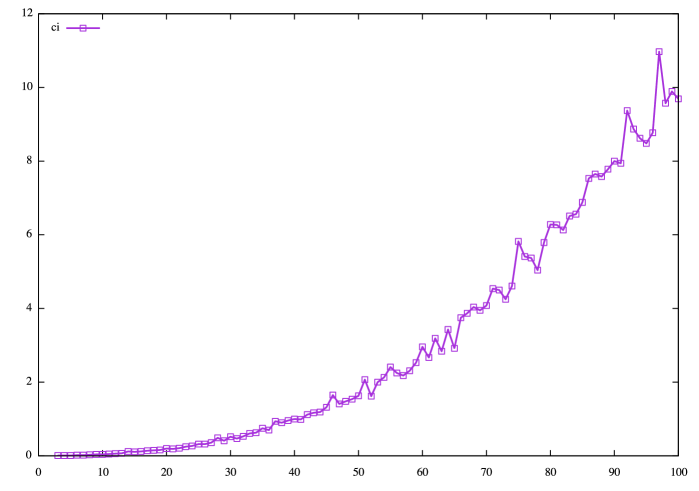
Figure 7: Dining Cryptographers experiments, optimized running times (s)

8.2 One-time Pad

The next example concerns message transmission using one-time pad encryption in the presence of an eavesdropper. Each instance has three agents (Alice, who sends an encrypted message to Bob, and Eve, who taps the wire). We scale the example by the length of the message, which is sent one bit at a time. For a message of length $n$, states have $O(n)$ variables. The protocol runs $2n$ steps, two for each bit. The formula is evaluated at time $2n$, and says that Eve does not learn the value of the first bit.

For this example, we found that the best performance for the unoptimized version was obtained using MCK version 0.5.1, which used a different encoding from more recent versions. Performance of model checking is shown in Table 2.

The running times for the optimized version grow very slowly (the numbers show a step-like behaviour due to rounding). Intuitively, the conditional independence optimization detects in this example that the first bit and the others are independent, and uses this to optimize the model checking computation. This means that for all $n$, the ultimate BDD model checking computation is performed on the same model for all $n$, and the primary running time cost lies in the generation of the dependence graph, and its analysis, that precedes the BDD computation. On the other hand, the unoptimized (xn) model checking running times show significant growth, with a large spike towards the end, where the speedup obtained from the optimization is over 10,000 times.

$n$ ci (s) xn (s) xn/ci 3 0.01 0.03 3 4 0.01 0.08 8 5 0.01 0.10 10 6 0.01 0.18 18 7 0.01 0.27 27 8 0.01 0.35 35 9 0.01 0.52 52 10 0.02 0.52 26 11 0.02 1.25 63 12 0.02 1.38 69 13 0.02 2.04 102 14 0.02 2.19 110 15 0.02 3.98 199 16 0.03 5.50 183 17 0.03 5.01 167 18 0.03 5.47 182 19 0.03 7.24 241 20 0.04 9.71 243 21 0.04 8.42 211 22 0.04 8.82 221 23 0.04 11.10 278 24 0.04 17.88 447 25 0.04 36.68 917 26 0.04 33.26 832 27 0.05 23.60 472 28 0.05 34.88 698 29 0.05 99.50 1990 30 0.05 50.10 1002 31 0.05 75.13 1503 32 0.05 67.37 1347 33 0.06 97.23 1621 34 0.06 184.19 3070 35 0.06 89.47 1491 36 0.07 131.74 1882 37 0.07 164.76 2354 38 0.07 259.48 3707 39 0.07 275.87 3941 40 0.07 749.88 10713

Table 2: One-time pad protocol, optimized and unoptimized running times, and speedup ratio, “single-bit” formula

8.3 Oblivious Transfer

The next example concerns an oblivious transfer protocol due to Rivest [25], which allows Bob to learn exactly one of Alice’s two messages $m_{0},m_{1}$, of his choice, without Alice knowing which message was chosen by Bob. Each instance has two agents, and we scale by the length of the message. For a message of length $n$, states have $O(n)$ variables. We consider two formulas for this protocol. Both are evaluated at time 3 in all instances.

The first formula says that if Bob chose to receive message $m_{1}$, then he does not learn the first bit of $m_{0}$. The running times for model checking this formula are given in Table 3. In this example, the conditional independence optimization gives a significant speedup, in the range of one to two orders of magnitude (more precisely, 12 to 221) improvement on the inputs considered, and increasing as the scale of the problem increases.

$n$ ci (s) xn (s) xn/ci 3 0.02 0.24 12 4 0.03 0.52 17 5 0.05 0.90 18 6 0.07 1.80 26 7 0.11 2.24 20 8 0.14 3.54 25 9 0.15 4.97 33 10 0.16 7.20 45 11 0.21 13.08 62 12 0.26 16.68 64 13 0.32 32.72 102 14 0.39 62.08 159 15 0.43 50.95 118 16 0.50 36.73 73 17 0.60 38.36 64 18 0.71 69.27 98 19 0.77 170.16 221 20 1.09 148.56 136

Table 3: Rivest Oblivious Transfer Protocol, optimized and unoptimized running times, and speedup ratio, “single-bit” formula

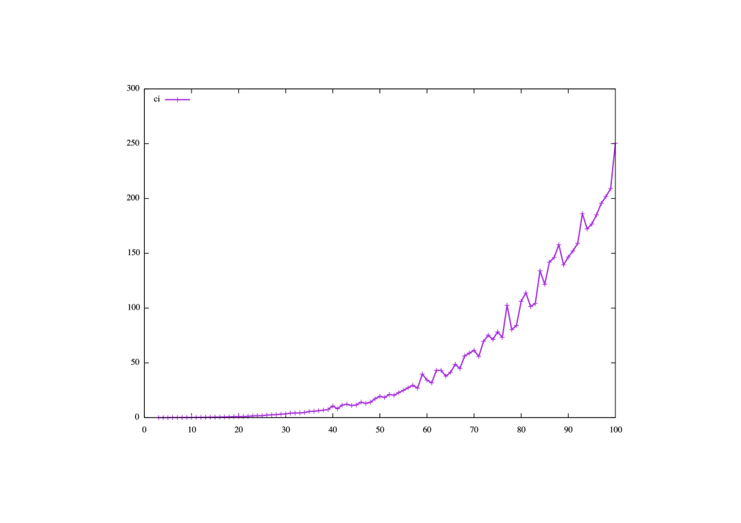
Figure 8: Oblivious transfer protocol experiments, optimized running times, “single-bit” formula

Running just the optimized version on larger instances, we obtain the plot shown in Figure 8. This shows that the optimization allows us to handle significantly larger instances: up to 97 agents can be handled in under 200 seconds, compared with 19 agents in 170 seconds unoptimized.

An example in which the optimization does not always yield a performance improvement arises when we change the formula model checked in this example to one that states that if Bob chose to receive $m_{1}$, then he does not learn the value of any bit of $m_{0}$. The running times are shown in Table 4.

$n$ ci (s) xn (s) xn/ci 3 0.03 0.25 8.3 4 0.05 0.51 10.2 5 0.12 0.86 7.2 6 0.15 1.58 10.5 7 0.25 2.84 11.4 8 0.42 3.52 8.4 9 0.50 5.11 10.2 10 0.55 7.79 14.2 11 1.18 13.07 11.1 12 3.72 14.63 3.9 13 5.20 39.74 7.6 14 7.13 48.64 6.8 15 4.91 56.62 11.5 16 20.16 38.09 1.9 17 32.95 42.40 1.3 18 174.96 86.81 0.5 19 229.85 96.86 0.4 20 342.40 184.08 0.5

Table 4: Rivest Oblivious Transfer Protocol, optimized and unoptimized running times, and speedup ratio, “all bits” formula

Here, the optimization initially gives a speedup of roughly one order of magnitude, but on the three largest examples, the performance of the unoptimized algorithm is better by a factor of two. The lower size of the initial speedup, compared to the first formula, can be explained from the fact that are obviously fewer variables that are independent of the second formula, since the formula itself contains more variables. (The “all bits” formula contains $O(n)$ rather than just one variable explicitly, but recall that knowledge operators implicitly introduce more variables, so the “first bit” formula implicitly has $O(n)$ variables.) It is not immediately clear exactly what accounts for the switchover.

8.4 Message Transmission

The next example concerns the transmission of a single bit message across a channel that is guaranteed to deliver it, but with uncertain delay This example has two agents Alice and Bob , and runs for $n+1$ steps, where $n$ is the maximum delay. States have $O(n)$ variables. The formula considered states at time $n+1$ that Alice knows that Bob knows … (nested five levels) that the message has arrived. Because of the nesting, the algorithm used in the unoptimized case is that invoked by the MCK construct spec_spr_nested – this essentially performs BDD-based model checking in a structure in which the worlds are runs of length equal to the maximum time relevant to the formula.

Table 5 compares the performance of the conditional independence optimization with this algorithm. The degree of optimization obtained is significant, increasing to over four orders of magnitude.

$n$ ci (s) nested(s) nested/ci 3 0.01 0.02 2 4 0.01 0.03 3 5 0.01 0.04 4 6 0.01 0.06 6 7 0.01 0.11 11 8 0.02 0.20 10 9 0.03 0.46 15 10 0.03 1.05 35 11 0.05 2.44 49 12 0.07 5.69 81 13 0.09 14.5 161 14 0.12 34.77 290 15 0.16 89.31 558 16 0.20 360.3 1802 17 0.27 1597.91 5918

Table 5: Message Transmission Protocol, optimized and unoptimized running times, and speedup ratio

Running the optimization for larger instances, we obtain the plot of running times in Figure 9. We again have that the optimization enables significantly larger instances to be handled in a given amount of time: as many as 65 agents in 342 seconds, compared to just 16 agents in 360 seconds for the unoptimized version.

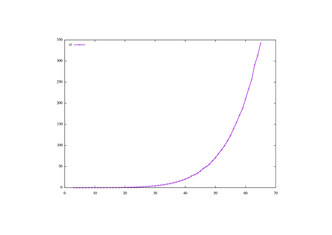
Figure 9: Message Transmission Protocol, optimized running times

8.5 Chaum’s two-phase protocol

The final example we consider is Chaum’s two-phase protocol [10], a protocol for anonymous broadcast that uses multiple rounds of the Dining Cryptographers protocol. Model checking of this protocol has previously been addressed in [1].

This example scales by both the number of agents and the number of steps of the protocol: with $n$ agents, the protocol runs for $O(n)$ steps, and each state is comprised of $O(n)$ variables. We check a formula with $O(n)$ variables that says that the first agent has a bit rcvd1 set to true at the end of the protocol iff it knows that some other agent is trying to send bit 1.

The protocol is more complex than the others considered above. An initial set of $n$ “booking” rounds of the Dining Cryptographers protocol is used to anonymously attempt to book one of $n$ slots, and this is followed by $n$ “slot” rounds of the Dining Cryptographers protocol, in which an agent who has booked a slot without detecting a collision with another agent’s booking, uses that slot to attempt to broadcast a message. Because undetected booking collisions remain possible, collisions might also be detected in the second phase. Because of the complexity of the protocol, this example can only be model checked on small instances in reasonable time, even with the optimization. Table 6 shows the running times obtained: for the unoptimized version, we again used MCK-0.5.1.

$n$ ci (s) xn (s) 3 0.04 0.79 4 0.11 96.47 5 0.49 $>$ 2 hrs 6 2.46 - 7 12.93 - 8 155.41 - 9 $>$ 2hrs -

Table 6: Chaum’s two-phase protocol, optimized and unoptimized running times

The running time of the unoptimized computation explodes at $n=5$ as we increase the number of agents. The optimized computation is significantly less, but also eventually explodes, at $n=9$. Thus, the optimization has doubled the size of the problem that can be handled in reasonable time.

9 Related Work and Conclusion

We conclude with a discussion of some related work and future directions.

Wilson and Mengin [34] have previously related modal logic to valuation algebra, but their definition requires that the marginalization of a Kripke structure have exactly the same set of worlds and equivalence relation, and merely restricts the assignment at each world, so their approach does not give the optimization that we have developed, and a model checking approach based on it would be less efficient than that developed in the present paper. They do not discuss conditional independence, which is a key part of our approach.

Also related are probabilistic programs, a type of program containing probabilistic choice statements, that sample from a specified distribution. The semantics of such programs is that they generate a probability distribution over the outputs. These programs may contain statements of the form $observe(\phi)$ where $\phi$ is a boolean condition: these are interpreted as conditioning the distribution constructed to that point on the condition $\phi$. Hur et al. [17] develop an approach to slicing probabilistic programs based on a static analysis that incorporates ideas from the Bayesian net literature. There are several differences between probabilistic programs and our work in this paper. One is that we deal with discrete knowledge rather than probability – in general, this makes our model checking problem more tractable. We also reason about all possible sequences of observations, rather than one particular sequence of observations. Additionally, we allow observations by multiple agents rather than just one. Finally, via knowledge operators, we have a locus of reference to observations in our framework that is located in formulas rather than inside the program – this enables us to ask multiple questions about a program without changing the code, whereas in probabilistic programs, one would need to handle this by multiple distinct modifications of the code.

The results of the present paper concern formulas that refer (directly and through knowledge operators) only to a specific time. Our approach, however, can be easily extended by means of a straightforward transformation to formulas that talk about multiple time points, and we intend to implement this extension in future work.

The technique we have developed can also be extended to deal with multi-agent models based on programs taking probabilistic transitions, which MCK already supports. Formulas in this extension would include operators that talk about an agent’s subjective probability, given what it has observed.

Other extensions we intend to implement are to enrich the range of knowledge semantics beyond the synchronous perfect recall semantics treated in this paper: essentially the same techniques will apply to the clock semantics (in which an agent’s knowledge is based on just its current observation and the current time). The observational semantics, in which the agent’s knowledge is based just on its current observation, will be more challenging, since it is asynchronous, and knowledge formulas may refer to times arbitrarily far into the future.

Finally, whereas the present paper concentrated on straightline programs, we intend to extend to a richer protocol format, including conditionals. In general, this extension will diminish the power of the equality optimization, and result in an increased set of dependencies in which many variables become dependent on a variable representing the program counter. However, some extensions will be more managable, e.g., one that requires conditionals and loops to be balanced in their timing (a restriction already used in work on computer security to avoid unwanted information leakages).

Appendix A Details of Experiments

In this appendix we provide further details on the examples considered in our experiments.

The MCK scripts below start with a declaration of global variables, followed by the “init_cond” construct which gives a boolean formula describing the initial states of the model. This is followed by the declaration of the agents in model. Each declaration names the agent, gives the name of the protocol it runs (in quotes), followed by the binding of the parameters of this protocol to environment variables. The protocols are listed last in the script. All of the agent protocols are straightline. The bracket notation “<| ... |>” delimits atomic actions. The contents of these brackets are a sequence of assignments that execute atomically, without consuming time.

The intuitive operational semantics of the scripts is that at time $n$, the agents activate the next such action in the sequence. These actions are performed in the order of the agents listed, followed by the sequence of assignments in the “transitions” clause, which intuitively, describes events that happen in the environment at each step. The resulting state is then taken to be the state at time $n+1$.

Specifications are listed using the construct “spec_spr”. Here the “spr” indicates that we are using a synchronous perfect recall semantics for knowledge.

A.1 Dining Cryptographers

The Dining Cryptographers protocol has already been discussed in the body of the paper, we provide the code for the 3-agent instance below. This example is generalized to larger instances by increasing the number $n$ of agents: each running the protocol given. The protocol can be run using any connected network, but we use a ring network, with agent $C_{i}$ sharing coins with agent $C_{i-1\mod n}$ to the left, and agent agent $C_{i+1\mod n}$ to the right. The query is stated in terms of the knowledge of agent $C_{0}$, and says that this agent either knows that nobody paid, knows that it paid itself, or knows that one of the other $n-1$ agents paid, but does not know which.

paid : Bool[3]
chan : Bool[3]
said : Bool[3]

init_cond =
((neg paid[1]) /\ (neg paid[2])) \/
((neg paid[0]) /\ (neg paid[2])) \/
((neg paid[0]) /\ (neg paid[1]))


agent C0 "dc_agent_protocol" (paid[0], chan[0], chan[1], said, said[0])

agent C1 "dc_agent_protocol" (paid[1], chan[1], chan[2], said, said[1])

agent C2 "dc_agent_protocol" (paid[2], chan[2], chan[0], said, said[2])

spec_spr_ci = X 3 (Knows C0 ((neg paid[0])  /\ (neg paid[1]) /\ (neg paid[2]))) \/
   (Knows C0 (paid[0]))  \/
   (Knows C0 ( False \/ paid[1]\/ paid[2])  /\
      (neg Knows C0 (neg paid[1]))/\ (neg Knows C0 (neg paid[2])))


protocol "dc_agent_protocol"
(
  paid : observable Bool,
  chan_left : Bool,
  chan_right : Bool,
  said : observable Bool[], -- the broadcast variables.
  say : Bool
)

coin_left : observable Bool
coin_right : observable Bool

begin
  <| chan_right := coin_right |>;
  <| coin_left := chan_left |>;
  <| say := coin_left xor coin_right xor paid |>  ;
  skip
end

A.2 One Time Pad

The one-time pad is a shared secret key to be used just once. It is known to give perfect encryption under this assumption. We model a system in which Alice has a message (a boolean string) to transmit to Bob. She is assumed to share a one-time pad, another boolean string of the same length as the message, with Bob. Alice encrypts her string by bitwise exclusive-or with the one-time pad, and sends the resulting encrypted bits via a channel that is observed by an eavesdropper Eve.

We parameterize this model by the length $n$ of the strings. The case of $n=3$ is shown below. We consider a query that states that at the end of the transmission, Eve does not know the value of the first bit of Alice’s message.

-- The ’secret’ one-time-pad shared between Alice and Bob.
one_time_pad : Bool[3]
-- The communications channel.
channel : Bool

agent Alice "sender"      (one_time_pad, channel)
agent Bob   "receiver"   (one_time_pad, channel)
agent Eve   "eavesdropper" (channel)

spec_spr  =
 X 6  ((neg (Knows Eve Alice.message[0])) /\ (neg (Knows Eve (neg Alice.message[0]))))

-- Alice’s protocol.
protocol "sender" (otp : Bool[3], chan : Bool)

message : Bool[3]
bit : Bool

begin
  <| bit := otp[0] |>; <| chan := message[0] xor bit |>;
  <| bit := otp[1] |>; <| chan := message[1] xor bit |>;
  <| bit := otp[2] |>; <| chan := message[2] xor bit |>
end

-- Bob’s protocol.
protocol "receiver" (otp : observable Bool[3], chan : observable Bool)
begin
skip; skip; skip;
skip; skip; skip
end

-- Eve’s protocol.
protocol "eavesdropper" (chan : observable Bool)

begin
skip; skip;  skip;
skip; skip; skip
end

A.3 Rivest’s Oblivious Transfer Protocol

Rivests Oblivious Transfer protocol [25] enables a receiver Bob to obtain exactly one of two distinct messages $m_{0}$, $m_{1}$ possessed by a sender Alice, without Alice learning which message Bob chose to receive. That is, Bob makes a choice $c$, and, at the end of the protocol, knows message $m_{c}$, but not the other message $m_{\overline{c}}$, without Alice learning the value of $c$.

An MCK model of the protocol in the case where the length of the message is 3 is given. The protocol requires that Alice and Bob start with some correlated randomness which can be provided by a trusted third party who does not need to be online during the running of the protocol. This trusted third party provides Alice with two random strings $r_{0},r_{1}$, and Bob with a random bit $d$ and the string $r_{d}$. We do not model this third party explicitly, but start a the state where Alice and Bob have received this information. (As with the Dining Cryptographers protocols above, we model random choices as nondeterministic choices.)

Bob and Alice then exchange some messages computed from the initial information. Bob first sends a bit $e$, and Alice responds with two strings $f_{0},f_{1}$ that encode $m_{0}$ and $m_{1}$. Bob is then able to compute his desired message $m_{c}$ in the third step of the protocol.

For this protocol, we scale our experiments by the length $n$ of the messages $m_{0},m_{1}$ (the protocol always runs in 3 steps, but the last step is a local computation by Bob, so does not affect the agent’s knowledge). We consider two formulas:

1. The first “[Single]” says that if Bob chose to receive $m_{1}$, then he does not learn the first bit of $m_{0}$. Because the protocol effectively operates independently on the bits of the various messages, we expect that the dependency analysis will detect this independence and give a significant speedup as the size of the messages increase.

2. The first “[Any]” says that if Bob chose to receive $m_{1}$, then he does not learn any bit of $m_{0}$. This involves $n$ variables, so it is not immediately clear whether we should expect any optimization.

-- Alice’s messages
m0: Bool[3]
m1: Bool[3]

-- A variable used by Bob to store the message received
mc: Bool[3]

-- initial randomness
r0 : Bool[3]
r1 : Bool[3]
rd : Bool[3]
d : Bool

f0 : Bool[3]
f1 : Bool[3]
e : Bool
c: Bool

init_cond =
-- Message rd is determined from r0,r1 and d.
( neg d => ((r0[0] <=> rd[0])  /\ (r0[1] <=> rd[1])  /\ (r0[2] <=> rd[2]) )) /\
        (d => ((r1[0] <=> rd[0])  /\ (r1[1] <=> rd[1])  /\ (r1[2] <=> rd[2]) )) /\
-- The random strings are distinct.
( neg (r0[0] <=> r1[0])  \/ neg (r0[1] <=> r1[1])  \/ neg (r0[2] <=> r1[2]) ) /\
-- The messages m0, m1 are distinct.
( neg (m0[0] <=> m1[0])  \/ neg (m0[1] <=> m1[1])  \/ neg (m0[2] <=> m1[2]) )

agent Alice "alice" (r0, r1, m0, m1, f0, f1, e)
agent Bob "bob" (e, rd, d, c, f0, f1, mc)


spec_spr =
"[Any]: after two steps, Bob does not know the value of any bit of m0"
X 2  ( c => (neg (Knows Bob m0[0]) /\ neg (Knows Bob neg m0[0]) /\
                   neg (Knows Bob m0[1]) /\ neg (Knows Bob neg m0[1]) /\
                   neg (Knows Bob m0[2]) /\ neg (Knows Bob neg m0[2])))

spec_spr =
"[Single]: after two steps, Bob does not know the value of the first bit of m0"
X 2  (neg (Knows Bob m0[0]) /\ neg (Knows Bob neg m0[0]))

spec_spr  = "[Alice] Alice does not learn Bob’s choice: "
X 3 ( (neg Knows Alice c) /\ (neg Knows Alice neg c ) )


protocol "alice" (r0 : observable Bool[3], r1: observable Bool[3],
                  m0 : observable Bool[3], m1: observable Bool[3],
                  f0 : observable Bool[3], f1: observable Bool[3],
                  e: observable Bool)

begin
  skip;
  <|
     f0[0]:= ( (neg e) /\ (m0[0] xor r0[0])) \/ (e /\ (m0[0] xor r1[0])) ;
     f1[0]:= ( (neg e) /\ (m1[0] xor r1[0])) \/ (e /\ (m1[0] xor r0[0])) ;

     f0[1]:= ( (neg e) /\ (m0[1] xor r0[1])) \/ (e /\ (m0[1] xor r1[1])) ;
     f1[1]:= ( (neg e) /\ (m1[1] xor r1[1])) \/ (e /\ (m1[1] xor r0[1])) ;

     f0[2]:= ( (neg e) /\ (m0[2] xor r0[2])) \/ (e /\ (m0[2] xor r1[2])) ;
     f1[2]:= ( (neg e) /\ (m1[2] xor r1[2])) \/ (e /\ (m1[2] xor r0[2]))
  |>;
  skip
end


protocol "bob" (e: Bool,
       rd: observable Bool[3], d: observable Bool, c: observable Bool,
       f0: observable Bool[3], f1: observable Bool[3], mc: observable Bool[3])
begin
 <| e:= d xor c |>;
 skip;
 <|
   mc[0]:= ((neg c) /\ (f0[0] xor rd[0])) \/ (c /\ (f1[0] xor rd[0])) ;
   mc[1]:= ((neg c) /\ (f0[1] xor rd[1])) \/ (c /\ (f1[1] xor rd[1])) ;
   mc[2]:= ((neg c) /\ (f0[2] xor rd[2])) \/ (c /\ (f1[2] xor rd[2]))
 |>
end

A.4 Message Transmission with Uncertain Delay

This example models a scenario where an agent Alice sends a message $x$ to Bob through a channel with a bounded delay. The example is parameterized by the maximum length $n$ of the delay. The instance with $n=3$ is shown.

Initially, all variables except Alice’s local variable $x$ and the array $\mathit{delay}$ are 0. At time $0$, Alice writes the message $x$ to a buffer, and at time $1$, Alice sets a bit to $\mathit{True}$ to start the transmission. The message is delivered as soon as the value $\mathit{delay}[0]$ is $\mathit{True}$. Here $\mathit{delay}$ is an array of length $n$, which initially has a random value. At each step, the values in the array shift to the left by one position, and the final value is set to be $\mathit{False}$. Thus, $\mathit{delay}[0]$ becomes $F$ by time $n$ at the latest, and the message is guaranteed to be delivered by time $n+1$.

In this example, we consider a query that involves nested knowledge. It is the case that Alice considers it possible up to time $n+1$ that the message has not yet been delivered, but by time $n+1$ Alice knows that the message must have been delivered. In fact, it is common knowledge at time $n+1$ that the message has been delivered. We consider a query that says that Alice Knows that Bob Knows that Alice Knows that Bob Knows that Alice Knows the message has been received by Bob.

delay : Bool[3]
outA : Bool
sentA : Bool

inB : Bool
rcdB : Bool

init_cond = neg (sentA \/ outA \/ inB \/ rcdB)

agent Alice "sender" (outA, sentA)
agent Bob  "receiver" (inB, rcdB)

transitions
begin
-- delay[0] captures whether transmission is delayed in the current step
-- if there is no delay and Alice has sent, then Bob receives

rcdB := rcdB \/ (neg delay[0] /\ sentA );
inB := (neg delay[0] /\ sentA /\ outA) \/ ((delay[0] \/ neg sentA) /\ inB);

-- delay starts out random, and shifts from right to left

delay[0] := delay[1] ;
delay[1] := delay[2];
delay[2] := False
 end

spec_spr = X 4 Knows Alice (Knows Bob (Knows Alice (Knows Bob (Knows Alice rcdB ))))

-- Alice’s protocol.
protocol "sender" (chan : Bool, sent : Bool )

x: Bool

begin
<| chan := x |> ;
<| sent := True |> ;
skip; skip; skip
end



-- Bob’s protocol.
protocol "receiver" (chanin: observable Bool, rcd: observable Bool)

begin
skip; skip; skip; skip
end

A.5 Two-Phase Protocol

In the Dining Cryptographers protocol, it is assumed that at most one agent wishes to communicate the message that they paid. The two-phase protocol, also from [10], is an application of the basic Dining Cryptographers protocol, in which multiple rounds of the basic dining cryptographers protocol are used to allow anonymous broadcast in a setting where multiple agents may have a message to send.

We model an abstraction of this protocol, in which the message of each agent consists of a single bit, and each application of Dining Cryptographers scheme is represented by taking the exclusive-or of the bits contributed to the round by each of the agents. It is shown in [1] that this abstraction is sound for verification of epistemic properties.

The protocol operates in two phases. The second phase consists of some number $m$ of rounds of the basic Dining Cryptographers protocol, which some agent may use to anonymously broadcast a message. Of course, to remain anonymous, the slot in which it chooses to broadcast must not be predictable, so the agent must choose its slot randomly. This creates the risk of collisions, in which two agents broadcast in the same slot. This is problematic: the Dining Cryptographers protocol assumes that at most one agent is sending a message.

To decrease the risk of a collision, in the first phase, any agent with a message to broadcast attempts to book one of the broadcast slots. To maintain its anonymity, the booking of a slot must also be done anonymously, and the Dining Cryptographers protocol is also used by the agent to announce that it wishes to use its chosen slot. Thus, the first phase also consists of $m$ rounds of the Dining Cryptographers protocol.

Some collisions can be detected during the first round – in particular, if an even number of agents attempt to book the same slot, they will detect the collision from the outcome of that booking round. There remains the possibility of undetected collisions — the idea of the protocol is that these will be detected during the transmission round, and that in this case, the agent will make another attempt to transmit in a later run of the protocol.

This makes the precise conditions under which it is known that a message has been successfully transmitted using the two-phase protocol quite subtle. For a longer discussion of the subtleties, see [1]. We focus on one of the simpler queries from that analysis, concerning whether an agent knows that some other agent is transmitting a particular bit.

In the script, the boolean array slotsC$i$ is used to represent which slot, if any, agent C$i$ has selected for its transmission; slotsC$i[0]$ represents that the agent has nothing to transmit. The initial condition states that at exactly one of slotsC$i[j]$ holds, for $j=0\ldots n$. The variables rr$i$ are used to capture the results of the reservation round $i$ during the first phase. These values are then used during the corresponding round of the transmission phase to determine whether a value has been received in that round. Variable rcvd$X$ for $X\in\{0,1\}$ is used to represent that a bit $X$ has been received.

This example scales by increasing the number of agents or increasing the number of available slots. We have experimented with two versions, one where the number of slots is fixed at 5, and we vary the number of agents, and another, where we vary the number of agents and keep this equal to the number of slots.

The query that we consider states that the variable rcvd1 corresponds precisely to the agent knowing that some agent is transmitting the bit $1$. (We verify this for agent C0, it holds for the others by symmetry.)

 type Slot = {0..3}
slotsC0 : Bool[Slot]
slotsC1 : Bool[Slot]
slotsC2 : Bool[Slot]
say : Bool[3]
round_result : Bool

 init_cond =
(neg (slotsC0[0] /\ slotsC0[1])) /\ (neg (slotsC0[0] /\ slotsC0[2])) /\
(neg (slotsC0[0] /\ slotsC0[3])) /\ (neg (slotsC0[1] /\ slotsC0[2])) /\
(neg (slotsC0[1] /\ slotsC0[3])) /\ (neg (slotsC0[2] /\ slotsC0[3])) /\
(neg (slotsC1[0] /\ slotsC1[1])) /\ (neg (slotsC1[0] /\ slotsC1[2])) /\
(neg (slotsC1[0] /\ slotsC1[3])) /\ (neg (slotsC1[1] /\ slotsC1[2])) /\
(neg (slotsC1[1] /\ slotsC1[3])) /\ (neg (slotsC1[2] /\ slotsC1[3])) /\
(neg (slotsC2[0] /\ slotsC2[1])) /\ (neg (slotsC2[0] /\ slotsC2[2])) /\
(neg (slotsC2[0] /\ slotsC2[3])) /\ (neg (slotsC2[1] /\ slotsC2[2])) /\
(neg (slotsC2[1] /\ slotsC2[3])) /\ (neg (slotsC2[2] /\ slotsC2[3])) /\
 (slotsC0[0] \/ slotsC0[1] \/ slotsC0[2] \/ slotsC0[3])  /\
 (slotsC1[0] \/ slotsC1[1] \/ slotsC1[2] \/ slotsC1[3])  /\
 (slotsC2[0] \/ slotsC2[1] \/ slotsC2[2] \/ slotsC2[3])

agent C0 "twophase_protocol" (slotsC0, say[0], round_result)
agent C1 "twophase_protocol" (slotsC1, say[1], round_result)
agent C2 "twophase_protocol" (slotsC2, say[2], round_result)

transitions
begin
round_result := say[0] xor say[1] xor say[2]
end

 -- rcvdX = I know someone else is sending X

spec_spr = X 13 C0.rcvd1 <=>
Knows C0 ((neg slotsC1[0] /\ C1.message) \/ (neg slotsC2[0] /\ C2.message))

protocol "twophase_protocol"
(
  slot_request: observable Bool[],
  say : Bool,
  round_result: observable Bool
)

-- the following variables are initialised nondeterministically:

-- the message the agent sends, if any
message : observable Bool

-- the result for each DC round
-- rri = message received in booking round i
rr1 : Bool
rr2 : Bool
rr3 : Bool

--  rcvdX = I know a message X has been sent by someone else
rcvd0 :  Bool
rcvd1 :  Bool



begin
-- reservation phase
-- time 0
<| say := slot_request[1] |>;

<| rr1 := round_result |>;

<| say := slot_request[2] |>;

<| rr2 := round_result |>;

<| say := slot_request[3] |>;

<| rr3 := round_result |>;

--initialize rcvd vars
<| rcvd0:= False ; rcvd1 := False |>;

 -- Sending phase:
<| say := (slot_request[1] /\ rr1 /\ message ) |> ;

<|
    rcvd1 := rcvd1 \/ (neg slot_request[1] /\ rr1 /\ round_result) \/
             (slot_request[1] /\ rr1 /\ (message xor round_result));

    rcvd0 := rcvd0 \/ (neg slot_request[1] /\ rr1 /\ neg round_result) \/
             (slot_request[1] /\ rr1 /\ (message xor round_result))
|> ;

<| say := (slot_request[2] /\ rr2 /\ message ) |> ;

<|
    rcvd1 := rcvd1 \/ (neg slot_request[2] /\ rr2 /\ round_result) \/
             (slot_request[2] /\ rr2 /\ (message xor round_result));

    rcvd0 := rcvd0 \/ (neg slot_request[2] /\ rr2 /\ neg round_result) \/
             (slot_request[2] /\ rr2 /\ (message xor round_result))
|> ;

<| say := (slot_request[3] /\ rr3 /\ message ) |> ;

<|
    rcvd1 := rcvd1 \/ (neg slot_request[3] /\ rr3 /\ round_result) \/
             (slot_request[3] /\ rr3 /\ (message xor round_result));

    rcvd0 := rcvd0 \/ (neg slot_request[3] /\ rr3 /\ neg round_result) \/
             (slot_request[3] /\ rr3 /\ (message xor round_result))
|>

end

References

- [1] O. I. Al-Bataineh and R. van der Meyden. Abstraction for epistemic model checking of dining cryptographers-based protocols. In Proc. of the 13th Conf. on Theoretical Aspects of Rationality and Knowledge (TARK-2011), pages 247–256, 2011.
- [2] O. Al Bataineh and R. van der Meyden. Epistemic model checking for knowledge-based program implementation: an application to anonymous broadcast. In SecureComm’10, 6th International ICST Conference on Security and Privacy in Communication Networks, 2010.
- [3] Kai Baukus and Ron van der Meyden. A knowledge based analysis of cache coherence. In Formal Methods and Software Engineering, 6th International Conference on Formal Engineering Methods, ICFEM 2004, Seattle, WA, USA, November 8-12, 2004, Proceedings, pages 99–114, 2004.
- [4] J. van Benthem. Modal correspondence theory. PhD thesis, Mathematish Instituut & Instituut voor Grondslagenonderzoek, University of Amsterdam, 1976.
- [5] U. Bertelè and F. Brioschi. Nonserial Dynamic Programming. Academic Press, 1972.
- [6] A. Biere, A. Cimatti, E. M. Clarke, O. Strichman, and Y. Zhu. Bounded model checking. Advances in Computers, 58:118–149, 2003.
- [7] Ioana Boureanu, Mika Cohen, and Alessio Lomuscio. Automatic verification of temporal-epistemic properties of cryptographic protocols. Journal of Applied Non-Classical Logics, 19(4):463–487, 2009.
- [8] Marco Bozzano, Alessandro Cimatti, Marco Gario, and Stefano Tonetta. Formal design of asynchronous fault detection and identification components using temporal epistemic logic. Logical Methods in Computer Science, 11(4), 2015.
- [9] J.R. Burch, E.M. Clarke, K.L. McMillan, D.L. Dill, and L.J. Hwang. Symbolic model checking: states and beyond. In Proc. Symposium on Logic in Computer Science, pages 428–439. IEEE, 1990.
- [10] D. Chaum. The dining cryptographers problem: Unconditional sender and recipient untraceability. Journal of Cryptology, pages 65–75, 1988.
- [11] Adnan Darwiche. A logical notion of conditional independence: Properties and application. Artif. Intell., 97(1-2):45–82, 1997.
- [12] Adnan Darwiche. Model-based diagnosis using structured system descriptions. J. Artif. Intell. Res. (JAIR), 8:165–222, 1998.
- [13] Ronald Fagin. Multivalued dependencies and a new normal form for relational databases. ACM Trans. Database Syst., 2(3):262–278, 1977.
- [14] P. Gammie and R. van der Meyden. MCK: Model checking the logic of knowledge. In Proc. 16th Int. Conf. on computer aided verification (CAV’04), volume 3114 of LNCS, pages 479–483. Springer-Verlag, 2004.
- [15] Xiaowei Huang, Patrick Maupin, and Ron van der Meyden. Model checking knowledge in pursuit evasion games. In IJCAI 2011, Proceedings of the 22nd International Joint Conference on Artificial Intelligence, Barcelona, Catalonia, Spain, July 16-22, 2011, pages 240–245, 2011.
- [16] Xiaowei Huang, Ji Ruan, and Michael Thielscher. Model checking for reasoning about incomplete information games. In AI 2013: Advances in Artificial Intelligence - 26th Australasian Joint Conference, Dunedin, New Zealand, December 1-6, 2013. Proceedings, pages 246–258, 2013.
- [17] Chung-Kil Hur, Aditya V. Nori, Sriram K. Rajamani, and Selva Samuel. Slicing probabilistic programs. In ACM SIGPLAN Conference on Programming Language Design and Implementation, PLDI’14, page 16, 2014.
- [18] J. Kohlas and P.P. Shenoy. Computation in valuation algebras. In Algorithms for Uncertainty and Defeasible Reasoning: Handbook of Defeasible Reasoning and Uncertainty Management Systems, volume 5, pages 5–39. Kluwer Academic Publishers, 2000.
- [19] D. Koller and N. Friedman. Probabilistic Graphical Models. MIT Press, 2009.
- [20] A. Kong. Multivariate Belief Functions and Graphical Models. PhD thesis, Department of Statistics, Harvard University, 1986.
- [21] Steffen L. Lauritzen, A. Philip Dawid, B. N. Larsen, and Hanns-Georg Leimer. Independence properties of directed markov fields. Networks, 20(5):491–505, 1990.
- [22] D. Maier. The Theory of Relational Databases. Computer Science Press, 1983.
- [23] S. Olmsted. On representing and Solving Decision Problems. PhD thesis, Dept. of Engineering-Economic Systems, Stanford University, 1983.
- [24] J. Pearl. Probabilistic Reasoning in Intelligent Systems: Networks of Plausible Inference. Morgan Kaufmann, San Mateo, CA, 1988.
- [25] Ronald L. Rivest. Unconditionally secure commitment and oblivious transfer schemes using private channels and a trusted initializer. Unpublished, but available at http://theory.lcs.mit.edu/~rivest/publications.html, November 1999.
- [26] P.P. Shenoy. A valuation-based language for expert systems. Int. J. of Approximate reasoning, 3:383–411, 1989.
- [27] P.P Shenoy. Valuation-based systems: A framework for managing uncertainty in expert systems. In L.A. Zadeh and J. Kacprzyk, editors, Fuzzy Logic for the Management of Uncertainty, pages 83–104. John Wiley and Sons, 1992.
- [28] P.P. Shenoy and G. Shafer. Axioms for probability and belief function propagation. In R.D. Shachter, T.S. Levitt, J.F. Lemmer, and L.N. Kanal, editors, Uncertainty in Artifical Intelligence, volume 4, pages 169–198. North Holland, 1990.
- [29] Fabio Somenzi. CUDD: CU decision diagram package. Available at http://vlsi.colorado.edu/~fabio/.
- [30] W. Spohn. Ordinal conditional functions: a dynamic theory of epistemic states. In W.L. Harper and B. Skyrms, editors, Causation in Decision, Belief Change, and Statistics, pages 105–134. Springer, 1988.
- [31] R. van der Meyden and K. Su. Symbolic model checking the knowledge of the dining cryptographers. In Proc. 17th IEEE Computer Security Foundation Workshop, pages 280–291. IEEE Computer Society, 2004.
- [32] Hans P. van Ditmarsch, Wiebe van der Hoek, Ron van der Meyden, and Ji Ruan. Model checking russian cards. Electr. Notes Theor. Comput. Sci., 149(2):105–123, 2006.
- [33] T. Verma and J.Pearl. Causal networks: Semantics and expressiveness. In Proc. 4th Workshop on Uncertainty in AI, pages 352–359, 1988.
- [34] Nic Wilson and Jérôme Mengin. Embedding logics in the local computation framework. Journal of Applied Non-Classical Logics, 11(3-4):239–261, 2001.