Semi-Coupled Two-Stream Fusion ConvNets
for Action Recognition at Extremely Low Resolutions

Abstract

Deep convolutional neural networks (ConvNets) have been recently shown to attain state-of-the-art performance for action recognition on standard-resolution videos. However, less attention has been paid to recognition performance at extremely low resolutions (eLR) (e.g., $16\times 12$ pixels). Reliable action recognition using eLR cameras would address privacy concerns in various application environments such as private homes, hospitals, nursing/rehabilitation facilities, etc. In this paper, we propose a semi-coupled, filter-sharing network that leverages high-resolution (HR) videos during training in order to assist an eLR ConvNet. We also study methods for fusing spatial and temporal ConvNets customized for eLR videos in order to take advantage of appearance and motion information. Our method outperforms state-of-the-art methods at extremely low resolutions on IXMAS ($93.7\%$) and HMDB ($29.2\%$) datasets.

1 Introduction

Human action and gesture recognition has received significant attention in computer vision and signal processing communities [21, 24, 29]. Recently, various ConvNet models have been applied in this context and achieved substantial performance gains over traditional methods that are based on hand-crafted features [9, 19]. Further improvements in the performance have been realized by using a two-stream ConvNet architecture [20] in which a spatial network concentrates on learning appearance features from RGB images while a temporal network takes optical flow snippets as input to learn dynamics. The final decision is made by averaging outputs of the two networks. More recent work [5, 11, 15] suggests fusion of spatial and temporal cues at an earlier stage so the appearance features are registered with motion features before the final decision. Results indicate that this approach improves action recognition performance.

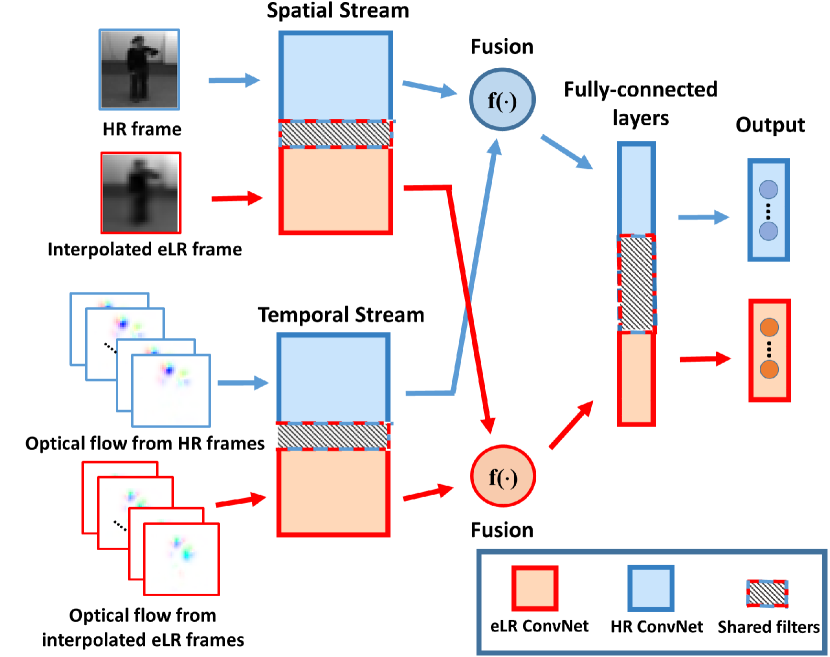
Figure 1: Diagram of the proposed ConvNet architecture. The blue blocks represent training-only HR information. The red blocks represent both training and testing eLR information. The overlap between the red and blue blocks indicates shared filters between eLR and HR information. Please note that both blocks use RGB and optical flow information.

As promising as these recent ConvNet-based models are, they typically rely upon data at about 200$\times$200-pixel resolution that is likely to reveal an individual’s identity. However, as more and more sensors are being deployed in our homes and offices, the concern for privacy only grows. Clearly, reliable methods for human activity analysis at privacy-preserving resolutions are urgently needed [2, 16]

Some of the early approaches to action recognition from eLR data use simple machine learning algorithms (e.g., nearest-neighbor classifier) [3] or leverage a ConvNet but only as an appearance feature extractor [17]. In very recent work [26], a partially-coupled super-resolution network (PCSRN) has been proposed for eLR image classification (not video). Basically, this network includes two ConvNets sharing a number of filters at each convolutional layer. While the input to one ConvNet consists of eLR images only, the input to the other network is formed from the corresponding HR images. The shared filters are trained to learn a nonlinear mapping between the eLR and HR feature spaces. Although this model has been designed for image recognition tasks, its excellent performance suggests that filter sharing could perhaps also benefit action recognition (from video) at extremely low resolutions.

In this paper, we combine the ideas of eLR-HR coupling and of two-stream ConvNets to perform reliable action recognition at extremely low resolutions. In particular, we adapt an existing end-to-end two-stream fusion ConvNet to eLR action recognition. We provide an in-depth analysis of three fusion methods for spatio-temporal networks, and compare them experimentally on eLR video datasets. Furthermore, inspired by the PCSRN model, we propose a semi-coupled two-stream fusion ConvNet that leverages HR videos during training in order to help the eLR ConvNet obtain enhanced discriminative power by sharing filters between eLR and HR ConvNets (Fig.1). Tested on two public datasets, the proposed model outperforms state-of-the-art eLR action recognition methods thus justifying our approach.

2 Related Work

ConvNets have been recently applied to action recognition and quickly yielded state-of-the-art performance. In the quest for further gains, a key question is how to properly incorporate appearance and motion information in a ConvNet architecture. In [7, 8, 22], various 3D ConvNets were proposed to learn spatio-temporal features by stacking consecutive RGB frames in the input. In [20], a novel two-stream ConvNet architecture was proposed which learns two separate networks: one dedicated to spatial RGB information, and another dedicated to temporal optical flow information. The softmax outputs of these two networks are later combined together to provide a final “joint” decision. Following this pivotal work, many works have extended the two-stream architecture such that only a single, combined network is trained. In [11], bilinear fusion was proposed in which the last convolutional layers of both networks are combined using an outer-product and pooling. Similarly, in [15] multiplicative fusion was proposed, and in [5] 3D convolutional fusion was introduced (incorporating an additional temporal dimension). However, all these methods were applied to standard-resolution video, and have not, to the best of our knowledge, been applied in the eLR context.

There have been few works that have addressed eLR in the context of visual recognition. In [26], very low resolution networks were investigated in the context of eLR image recognition. The authors proposed to incorporate HR images in training to augment the learning process of the network through filter sharing (PCSRN). In [3], eLR action recognition was first explored using $l_{1}$ nearest-neighbor classifiers to discriminate between action sequences. More recently, egocentric eLR activity recognition was explored in [17]. The authors introduced inverse super resolution (ISR) to learn an optimal set of image transformations during training that generate multiple eLR videos from a single HR video. Then, they trained a classifier based on features extracted from all generated eLR videos. The per-frame features include histogram of pixel intensities, histogram of oriented gradients (HOG) [4], histogram of optical flow (HOF) [1] and ConvNet features. To capture temporal changes, they used the Pooled Time Series (POT) feature representation [18] which is based on time-series analysis. This classifier was finally used in testing. However, in keeping with recent research trends our aim is to develop an end-to-end, ConvNet-only solution that avoids hand-crafted features and, therefore, minimizes human intervention. We benchmark our proposed methodologies against last two works, and show consistent recognition improvement.

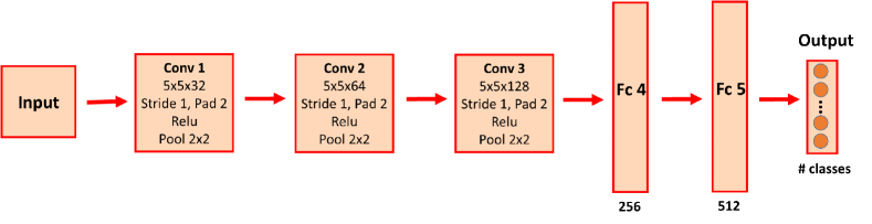
Figure 2: Basic ConvNet used in our model. The spatial and temporal streams have the same architecture except that the input dimension is larger in the temporal stream (the input to the temporal stream is a stacked optical flow). In our two-stream fusion ConvNets, two base ConvNets are fused after either the “Conv3” or “Fc4” layer.

3 Technical Approach

In this section, we propose two improvements to the two-stream architecture in the context of eLR. First, we explore methods to fuse the spatial and temporal networks, which allows subsequent layers to amplify and leverage joint spatial and temporal features. Second, we propose using semi-coupled networks which leverage HR information in training to learn transferable features between HR and eLR frames, resembling domain adaptation, in both the spatial and temporal streams.

3.1 Fusion of the two-stream networks

Multiple works have extended two-stream ConvNets by combining the spatial and temporal cues such that only a single, combined network is trained [5, 11, 15]. This is most frequently done by fusing the outputs of the spatial and temporal network’s convolution layers with the purpose of learning a correspondence of activations at the same pixel location. In this section, we discuss three fusion methods that we explore and implement in the context of eLR.

In general, fusion is applied between a spatial ConvNet and a temporal ConvNet. A fusion function $f$: $f(\boldsymbol{x}_{s}^{n},\boldsymbol{x}_{t}^{n})\rightarrow\boldsymbol{y}^{n}$ fuses spatial features at the output of the $n$-th layer $\boldsymbol{x}_{s}^{n}\in\mathbb{R}^{H_{s}^{n}\times W_{s}^{n}\times D_{s}^{n}}$ and temporal features at the output of the $n$-th layer $\boldsymbol{x}_{t}^{n}\in\mathbb{R}^{H_{t}^{n}\times W_{t}^{n}\times D_{t}^{n}}$ to produce the output features $\boldsymbol{y}^{n}\in\mathbb{R}^{H_{o}^{n}\times W_{o}^{n}\times D_{o}^{n}}$, where $H$, $W$, and $D$ represent the height, width and the number of channels respectively. For simplicity, we assume $H_{o}=H_{s}=H_{t},W_{o}=W_{s}=W_{t}$, and $D_{s}=D_{t}$ ($D_{o}$ is defined below). We discuss the fusion function for three possible operators:

Sum Fusion: Perhaps the simplest fusion strategy is to compute the summation of two feature maps at the same pixel location $(i,j)$ and the same channel $d$:

$$\boldsymbol{y}^{n,sum}(i,j,d)=\boldsymbol{x}_{s}^{n}(i,j,d)+\boldsymbol{x}_{t}^{n}(i,j,d)$$ (1)

where $1\leq i\leq H_{o}$ , $1\leq j\leq W_{o}$, $1\leq d\leq D_{o}$ ($D_{o}=D_{s}=D_{t}$) and $\boldsymbol{x}_{s}^{n}$, $\boldsymbol{x}_{t}^{n}$, $\boldsymbol{y}^{n}\in\mathbb{R}^{H_{o}\times W_{o}\times D_{o}}$. The underlying assumption of summation fusion is that the spatial and temporal feature maps from the same channel will share similar contexts.

Concat Fusion: The second fusion method we consider is a concatenation of two feature maps at the same spatial location $(i,j)$ across channel $d$:

$$\boldsymbol{y}^{n,cat}(i,j,2d)=\boldsymbol{x}_{s}^{n}(i,j,d),\$$ (2)

$$\boldsymbol{y}^{n,cat}(i,j,2d+1)=\boldsymbol{x}_{t}^{n}(i,j,d)$$ (3)

where $\boldsymbol{y}^{n,cat}\in\mathbb{R}^{H_{o}\times W_{o}\times D_{o}}$, $D_{o}=D_{s}+D_{t}$. Unlike the summation fusion, the concatenation fusion does not actually blend the feature maps together.

Conv Fusion: The third fusion operator we explore is convolutional fusion. First, $\boldsymbol{x}_{s}^{n}$ and $\boldsymbol{x}_{t}^{n}$ are concatenated as shown in (2, 3). Then, the stacked up feature map is convolved with a bank of filters $\mathcal{F}\in\mathbb{R}^{1\times 1\times D_{o}\times D^{\prime}_{o}}$ as follows:

$$\boldsymbol{y}^{n,conv}=\boldsymbol{y}^{n,cat}*\mathcal{F}+b,$$ (4)

where $b\in\mathbb{R}^{D^{\prime}_{o}}$ is a bias term. The filters have dimensions $1\times 1\times D_{o}$, $D_{o}=D_{s}+D_{t}$ and are used to learn weighted combinations of feature maps $\boldsymbol{x}_{s}^{n},\boldsymbol{x}_{t}^{n}$ at a shared pixel location. For our experiments, we have set the number of filters to $D^{\prime}_{o}=0.5\times D_{o}$.

Note, that regardless of the chosen fusion operator, the network will select filters throughout the entire network so as to minimize loss, and optimize recognition performance. Also, we would like to point out that other fusion operators, such as max, multiplication, and bilinear fusion [11], are possible, but have been shown in [5] to perform slightly worse than the operators we’ve discussed. Finally, it is worth noting that the type of fusion operation and the layer in which it occurs have a significant impact on the number of parameters. The number of parameters can be quite small if fusion across networks occurs in early layers. For example, convolutional fusion requires additional parameters since introducing a convolutional layer requires more filters. Regarding where to fuse the two networks, we adopt the convention used in [5] to fuse the two networks after their last convolutional layer (see Fig.3). We later report the results of fusion after the last convolutional layer (Conv3) and the first fully-connected layer (Fc4) and contrast their classification performance.

3.2 Semi-coupled networks

Applying recognition directly to eLR video is not robust as visual features tend to carry little information [26]. However, it is possible to augment ConvNet training with an auxiliary, HR version of the eLR video, but only use an eLR video in testing.

Figure 3: Visualization of the proposed semi-coupled networks of two fused two-stream ConvNets for video recognition. We feed HR RGB and optical flow frames ($32\times 32$ pixels) to the HR ConvNet (colored in blue). We feed eLR RGB ($16\times 12$ interpolated to $32\times 32$ pixels) and optical flow frames (computed from the interpolated $32\times 32$ pixel RGB frames) to the eLR ConvNet (colored in red). In training, the two ConvNets share $k^{n}$ ($n=1,...,5$) filters (gray shaded) between corresponding convolutional and fully-connected layers. Note that the deeper the layer, the more filters are being shared. In testing, we decouple the two ConvNets and only use the eLR network (the red network which includes the shared filters).

In this context, we propose to use semi-coupled networks which share filters between an eLR and an HR fused two-stream ConvNets. The eLR two-stream ConvNet takes an eLR RGB frame and its corresponding eLR optical flow frames as input. As we will discuss later, each RGB frame corresponds to multiple optical flow frames. The eLR RGB frames are interpolated to $32\times 32$ pixels from their original $16\times 12$ resolution. The eLR optical flow is computed from the interpolated $32\times 32$ eLR RGB frames. The HR two-stream ConvNet simply takes HR RGB and its corresponding HR optical flow frames of size $32\times 32$ as input. In layer number $n$ of the network $(n=1,\ldots,5)$, the eLR and HR two-stream ConvNets share $k^{n}$ filters. During training, we leverage both eLR and HR information, and update the filter weights of both networks in tandem. During testing, we decouple these two networks and only use the eLR network which includes shared filters. This entire process is illustrated in Fig. 3.

The motivation for sharing filters is two-fold: first, sharing resembles domain adaptation, aiming to learn transferable features from the source domain (eLR images) to the target domain (HR images); second, sharing can be viewed as a form of data augmentation with respect to the original dataset, as the shared filters will see both low and high resolution images (doubling the number of training inputs). However, it is important to note that in practice, as shown in [13], the mapping between eLR and HR feature space is difficult to learn. As a result, the feature space mapping between resolutions may not fully overlap or correspond properly to one-another after learning. To address this, we intentionally leave a number of filters ($D^{n}-k^{n}$) unshared in layer $n$, for each $n$. These unshared filters will learn domain-specific (resolution specific) features, while the shared filters learn the nonlinear transformations between spaces. To implement this filter sharing paradigm, we alternate between updating the eLR and HR two-stream ConvNets during training. Let $\boldsymbol{\theta}_{\text{eLR}}$ and $\boldsymbol{\theta}_{\text{HR}}$ denote the filter weights of the eLR and the HR two-stream ConvNets. These two filters are composed of three types of weights: $\boldsymbol{\theta}_{\text{shared}}$, the weights that are shared between both the eLR and HR networks, and $\boldsymbol{\theta}_{\text{eLR}^{*}}$, $\boldsymbol{\theta}_{\text{HR}^{*}}$, the weights that belong to only the eLR or the HR network, respectively. With these weights, we update both networks as follows:

$$\boldsymbol{\theta}_{\text{eLR}}^{m}=\left[\begin{array}[]{c}\boldsymbol{\theta}_{\text{eLR}^{*}}^{m-1}+\mu\dfrac{\partial\boldsymbol{L}_{\text{eLR}}^{m-1}}{\partial\boldsymbol{\theta}_{\text{eLR}^{*}}^{m-1}}\\ \\ \boldsymbol{\theta}_{\text{shared}}^{2m-2}+\mu{\dfrac{\partial\boldsymbol{L}_{\text{eLR}}^{m-1}}{\partial\boldsymbol{\theta}_{\text{shared}}^{2m-2}}}\end{array}\right]$$ (5)

$$\boldsymbol{\theta}_{\text{HR}}^{m}=\left[\begin{array}[]{c}\boldsymbol{\theta}_{\text{HR}^{*}}^{m-1}+\mu{\dfrac{\partial\boldsymbol{L}_{\text{HR}}^{m-1}}{\partial\boldsymbol{\theta}_{\text{HR}^{*}}^{m-1}}}\\ \\ \boldsymbol{\theta}_{\text{shared}}^{2m-1}+\mu{\dfrac{\partial\boldsymbol{L}_{\text{HR}}^{m-1}}{\partial\boldsymbol{\theta}_{\text{shared}}^{2m-1}}}\end{array}\right]$$ (6)

where $\mu$ is the learning rate, $m$ is the training iteration, and $\boldsymbol{L}_{\text{eLR}}$ and $\boldsymbol{L}_{\text{HR}}$ are, respectively, the loss functions of each network. In each training iteration, the shared weights are updated in both the eLR and the HR ConvNet, i.e., they are updated twice in each iteration. Specifically, in each training iteration $m$, we have

$$\boldsymbol{\theta}_{\text{shared}}^{2m-1}=\boldsymbol{\theta}_{\text{shared}}^{2m-2}+\mu{\dfrac{\partial\boldsymbol{L}_{\text{eLR}}^{m-1}}{\partial\boldsymbol{\theta}_{\text{shared}}^{2m-2}}}$$ (7)

$$\boldsymbol{\theta}_{\text{shared}}^{2m-2}=\boldsymbol{\theta}_{\text{shared}}^{2m-3}+\mu{\frac{\partial\boldsymbol{L}_{\text{HR}}^{m-2}}{\partial\boldsymbol{\theta}_{\text{shared}}^{2m-3}}}$$ (8)

However, the resolution-specific unshared weights are only updated once: either in the eLR ConvNet training update or in the HR ConvNet training update. Therefore, the shared weights are updated twice as often as the unshared weights.

Our approach has been inspired by Partially-Coupled Super-Resolution Networks (PCSRN) [26] where it was shown that leveraging HR images in training of such networks can help discover discriminative features in eLR images that would otherwise have been overlooked during image classification. PCSRN is a super-resolution network that pre-trains network weights using filter sharing. This pre-training is intended to minimize the MSE of the output image and the target HR image via super-resolution. In our approach, we differ from this work by leveraging HR information throughout the entire training process. Our method does not need to pre-train the network; instead, we learn the entire network from scratch, and minimize the classification loss function directly while still incorporating HR information as shown in the equations above. Overall, we extend this model in two aspects: first, we consider shared filters in the fully-connected layers (previously only convolutional layers were considered for filter sharing). Second, we adapt this method for action recognition in fused two-stream ConvNets. We also report results for semi-coupled two-stream ConvNets across various fusion operators.

3.3 Implementation details

Two-stream fusion network. Conventional standard-resolution ConvNet architectures can be ill-suited for eLR images due to large receptive fields that can sometimes be larger than the eLR image itself. To address this issue, we have designed an eLR ConvNet consisting of 3 convolutional layers, and 2 fully-connected layers as shown in Fig. 2. We have tried many variations, but found that larger models do not improve performance. Also, the model in [17] is larger than ours, but achieves lower CCR. We base both our spatial and temporal streams on this ConvNet, and explore fusion operations after either the “Conv3” or “Fc4” layer. We train all networks from scratch using the Matconvnet toolbox [23]. The weights are initialized to be zero-mean Gaussian with a small standard deviation of $10^{-3}$. The learning rate starts from $0.05$ and is reduced by a factor of 10 after every 10 epochs. Weight decay and momentum are set to 0.0005 and 0.9 respectively. We use a batch size of 256 and perform batch normalization after each convolutional layer. At every iteration, we perform data augmentation by allowing a 0.5 probability that a given image in a batch is reflected across the vertical axis. Each RGB frame in the spatial stream corresponds to 11 stacked frames of optical flow. This stacked optical-flow block contains the current, the 5 preceding, and 5 succeeding optical flow frames. To regularize these networks during training, we set the dropout ratio of both fully-connected layers to 0.85.

Semi-coupled ConvNets. In Section 3.2, we have discussed how to incorporate filter sharing in a semi-coupled network. However, it is not obvious how many filters should be shared in each layer. To discover the proper proportion of filters we should share, we conducted a coarse grid search for the coupling ratio $c_{n}$ from 0 to 1 with a step size of $0.25$. The coupling ratio is defined as:

$$c_{n}=\frac{k^{n}}{D^{n}},\quad n=1,\cdots,5$$ (9)

where the two ConvNets are uncoupled when $c_{n}=0$ $(n=1,\cdots,5)$. For the step sizes that we consider, a brute force approach would be unfeasible, as the total number of two-stream networks to train would be $5^{5}=3125$. Therefore, we follow the methodology used in [26] to monotonically increase the coupling ratios with the increasing layer depth. This is inspired by the notion that the disparity between eLR and HR domains is reduced as the layer gets deeper [6, 25]. For all our experiments, we used the following coupling ratios: $c_{1}=0$, $c_{2}=0.25$, $c_{3}=0.5$, $c_{4}=0.75$, and $c_{5}=1$. We determined these ratios by performing a coarse grid search on a cross-validated subset of the IXMAS dataset (subjects 2, 4, 6).

Normalization. In our experiments, we apply a variant of mean-variance normalization to each video $v_{i,j}[t],i,j=1,\cdots,R,t=1,\cdots,T$, where $R$ is the spatial size, $T$ is the temporal length, and $v_{i,j}[t]$ denotes the grayscale value of pixel $(i,j)$ at time $t$, as follows:

$$\hat{v}_{i,j}[t]=\frac{v_{i,j}[t]-\mu_{i,j}}{\sigma}.$$ (10)

Above, $\mu_{i,j}$ denotes the empirical mean pixel value across time for the spatial location $(i,j)$, and $\sigma$ denotes the empirical standard deviation across all pixels in one video. The subtraction of the mean emphasizes a subject’s local dynamics, while the division by the empirical standard deviation compensates for the variability in subject’s clothing.

Optical flow. As discussed earlier, we use a stacked block of optical flow frames as input to the temporal stream. We follow [28] and use colored optical-flow frames. First, we compute optical flow between two consecutive normalized RGB frames [12]. The computed optical flow vectors are then mapped into polar coordinates and converted to hue and saturation based on the magnitude and orientation, respectively. The brightness is set to one. As a reminder, the eLR optical flow is computed from the interpolated $32\times 32$ pixel eLR frames. Further, we subtract the mean of the stacked optical flows to compensate for global motion as suggested in [20].

Source code: More implementation details as well as source code are available on project web site [code].

4 Experiments

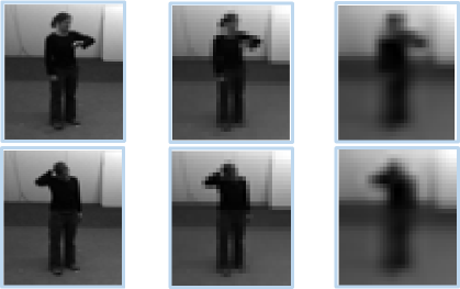
(a) IXMAS

(b) HMDB

Figure 4: Sample frames from IXMAS and HMDB datasets. (a) From left to right are original frames, and resized $32\times 32$ and $16\times 12$ frames from the IXMAS dataset. (b) From left to right are original frames, and resized $32\times 32$ and $12\times 16$ frames from the HMDB dataset. Note that we resize the IXMAS dataset to $16\times 12$ and the HMDB dataset to $12\times 16$ in order to preserve the original aspect ratio. We use $32\times 32$ resized videos as HR data. The $16\times 12$ ($12\times 16$) eLR videos are upscaled using bi-cubic interpolation to $32\times 32$ interpolated-eLR video which is used in our proposed semi-coupled fused two-stream ConvNet architecture.

4.1 Datasets

In order to confirm the effectiveness of our proposed method, we conducted experiments on two publicly-available video datasets. First, we use the ROI sequences from the multi-view IXMAS action dataset, where each subject occupies most of the field of view [27]. This dataset includes 5 camera views, 12 daily-life motions each performed 3 times by 10 actors in an indoor scenario. Overall, it contains 1,800 videos. To generate the eLR videos (thus eLR-IXMAS), we decimated the original frames to $16\times 12$ pixels and then upscaled them back to $32\times 32$ pixels by bi-cubic interpolation (Fig. 4). The upscaling operation does not introduce new information (fundamentally, we are still working with $16\times 12$ pixels) but ensures that eLR frames have enough spatial support for hierarchical convolutions to facilitate filter sharing. On the other hand, we generate the HR data by decimating the original frames straight to $32\times 32$ pixels. We perform leave-person-out cross validation in each case and compute correct classification rate (CCR) and standard deviation (StDev) to measure performance.

We also test our algorithm on the popular HMDB dataset [10] used for video activity recognition. The HMDB dataset consists of 6,849 videos divided into 51 action categories, each containing a minimum of 101 videos. In comparison to IXMAS, which was collected in a controlled environment, the HMDB dataset includes clips from movies and YouTube videos, which are not limited in terms of illumination and camera position variations. Therefore, HMDB is a far more challenging dataset, especially when we decimate to eLR, which we herein refer to as eLR-HMDB. In our experiments, we used the three training-testing splits provided with this dataset. Note that since there are 51 classes in the HMDB dataset, the CCR based on a purely random guess is $1.96\%$.

4.2 Results for eLR-IXMAS

We first conduct a detailed evaluation of the proposed paradigms on the eLR-IXMAS action dataset. For a fair comparison, we follow the image resolution, pre-processing and cross-validation as described in [3]. We first resize all video clips to a fixed temporal length $T=100$ using cubic-spline interpolation.

Table 1 summarizes the action recognition accuracy on the eLR-IXMAS dataset. We report the CCR for separate spatial and temporal ConvNets, as well as for various locations and operators of fusion, with and without eLR-HR coupling. We also report the baseline result from [3] which employs a nearest-neighbor classifier.

Table 1: Performance of different ConvNet architectures against baseline on the eLR-IXMAS dataset. “Spatial & Temp avg” has been performed by averaging the temporal and spatial stream predictions. The best performing method is highlighted in bold.

Method	Fusion Layer	eLR-HR	CCR	StDev
		coupling?
Baseline (Dai [3])	-	-	$80.0\%$	$6.9\%$
Spatial Network	-	No	$88.6\%$	$6.2\%$
Temporal Network	-	No	$91.6\%$	$4.9\%$
Spatial$\&$Temp avg	Softmax	No	$92.0\%$	$6.0\%$
Concat Fusion	Fc 4	No	$92.2\%$	$5.2\%$
	Fc 4	Yes	$92.5\%$	$5.5\%$
	Conv 3	No	$92.2\%$	$5.2\%$
	Conv 3	Yes	$93.3\%$	$5.6\%$
Conv Fusion	Fc 4	No	$92.0\%$	$5.8\%$
	Fc 4	Yes	$93.1\%$	$5.2\%$
	Conv 3	No	${93.3\%}$	${4.0\%}$
	Conv 3	Yes	$\mathbf{93.7\%}$	$\mathbf{4.5\%}$
Sum Fusion	Fc 4	No	$92.2\%$	$5.5\%$
	Fc 4	Yes	$92.8\%$	$7.1\%$
	Conv 3	No	$93.0\%$	$4.7\%$
	Conv 3	Yes	$93.6\%$	$4.0\%$

(a) eLR-IXMAS pixel-wise time series features [3]

(b) eLR-IXMAS ConvNet features after ‘Fc 5’ layer

Figure 5: 2-D t-SNE embeddings [14] of features for the eLR-IXMAS dataset. A single marker represents a single video clip and is color-coded by action type. (a) Embeddings of pixel-wise time series features [3]. (b) Embeddings of the last fully-connected layer’s output from our best performing ConvNet.

We first observe that dedicated spatial or temporal ConvNet outperforms the benchmark result from [3] by $8.6\%$ and $11.6\%$ respectively, which validates the discriminative power of a ConvNet. If we equally weigh these two streams (“Spatial&Temp avg”), we can see that the fusion only marginally improves recognition performance. Secondly, we can see that fusing after the “Conv3” layer provides a consistently better performance than fusing after the “Fc4” layer. In our preliminary experiments, we also found that fusing after the “Conv3” layer was consistently better than fusing after the “Conv2” layer, which suggests that there is an ideal depth (which is not too shallow or too deep in the network) for fusion. Regarding which fusion operator to use, we note that all 3 operators we consider provide comparable performance after the “Fc4” layer. However, if we fuse after the “Conv3” layer, convolutional fusion performs best.

As for the effectiveness of semi-coupling in the networks using HR information, we can see that eLR-HR coupling consistently improves recognition performance. Our best result on IXMAS is $93.7\%$, where we find that without coupling, our performance drops by $0.4\%$. This result is very close to that achieved by using only HR data in both training and testing, which is $94.4\%$ CCR. Effectively, this should be an upper-bound, in terms of performance, when using eLR-HR coupling in training but testing only on eLR data. That the performance gap between HR and eLR is small may be explained by the distinctiveness of actions and the controlled indoor environment (static cameras, constant illumination, etc.) in the IXMAS dataset. Additionally, the fine details (e.g., hair, facial features), that are only visible in HR, are not critical for action recognition.

In order to qualitatively evaluate our proposed model, we visualize various feature embeddings for the eLR-IXMAS dataset. We extract output features of the “Fc5” layer from the best-performing ConvNet (shown in bold), and project them to 2-dimensional space using t-SNE [14]. For comparison, we also apply t-SNE to the pixel-wise time series features proposed in our benchmark [3]. As seen in Fig. 5, the feature embedding from our ConvNet model is visually more separable than that of our baseline. This is not surprising, as we are able to consistently outperform the baseline on the eLR-IXMAS dataset.

Table 2: Comparison of the number of parameters of our best-performing action recognition ConvNet as compared to those of the standard-resolution image classification ConvNets.

Network	Task	Input resolution	$\#$ param
Ours	Action Rec.	$32\times 32\times 3$	0.84M
AlexNet	Image Class.	$224\times 224\times 3$	60M
VGG-16	Image Class.	$224\times 224\times 3$	138M
VGG-19	Image Class.	$224\times 224\times 3$	144M

Regarding the number of parameters, our ConvNet designed for eLR videos needs about 100 times less parameters than state-of-the art ConvNets designed for image classification like AlexNet [9], VGG-16, and VGG-19 [21] (Table 2). In consequence, this significantly reduces the computation cost of training and testing compared to these standard-resolution networks.

4.3 Results for eLR-HMDB

We also report the results of our methods on eLR-HMDB. Note that, for this dataset, we only report results for fusion after the “Conv3” layer, based on our observations from eLR-IXMAS. We follow the same pre-processing procedure as used for eLR-IXMAS except that we do not resize the video clips temporally for the purpose of having a fair comparison with the results reported in [17]. Our reported CCR is an average across the three training-testing splits provided with this dataset.

First, we measure the performance of a dedicated spatial-stream ConvNet and a dedicated temporal-stream ConvNet. As shown in Table 3, using only the appearance information (spatial stream) provides $19.1\%$ accuracy. If optical flow is used alone (temporal stream), performance drops to $18.3\%$. This is likely because videos in the HMDB dataset are unconstrained; camera movement is not guaranteed to be well-behaved, thus resulting in drastically different optical-flow quality across videos. Such variations are likely to be amplified in eLR videos. We then evaluate the same three fusion operators after the “Conv3” layer. Not surprisingly, compared to the average of predictions from a dedicated spatial network and a dedicated temporal network, fusing the temporal and spatial streams improves the recognition performance by $0.8\%$, $0.9\%$ and $1.8\%$ with concatenation, convolution, and sum fusion, respectively. Fusion alone does not bring significant improvement. This, however, is consistent with the observations in [5].

Table 3: Performance of different ConvNet architectures and current state-of-the-art method on the eLR-HMDB dataset. The two-stream networks are all fused after the “Conv3” layer. The best method is highlighted in bold.

Method	eLR-HR	CCR
	coupling?
Spatial Network	No	$19.1\%$
Temporal Network	No	$18.3\%$
Spatial $\&$ Temp avg	No	$19.6\%$
Concat Fusion	No	$20.4\%$
	Yes	$27.1\%$
Conv Fusion	No	${20.5\%}$
	Yes	$27.3\%$
Sum Fusion	No	$21.4\%$
	Yes	$\mathbf{29.2}\%$
ConvNet feat	-	$18.9\%$
+ SVM[17]
ConvNet feat	-	$20.8\%$
+ ISR + SVM[17]
ConvNet + hand-crafted feat	-	$28.7\%$
+ ISR + SVM[17]

When fusion is combined with eLR-HR coupling, the gains are significant. We achieve large performance gains from $20.4\%$ to $27.1\%$ using concatenation fusion, $20.5\%$ to $27.3\%$ using convolutional fusion, and $21.4\%$ to $29.2\%$ using sum fusion. Such notable improvements validate the discriminative capabilities of semi-coupled fused two-stream ConvNets. Compared to the state-of-the-art results reported in [17], our approach is able to outperform their ConvNet feature-only method by $8.4\%$. We also exceed the performance of their best method, that uses an augmented hand-crafted feature vector, by $0.5\%$.

5 Conclusion

In this paper, we proposed multiple, end-to-end ConvNets for action recognition from extremely low resolution videos (e.g., $16\times 12$ pixels). We proposed multiple eLR ConvNet architectures, each leveraging and fusing spatial and temporal information. Further, in order to leverage HR videos in training we incorporated eLR-HR coupling to learn an intelligent mapping between the eLR and HR feature spaces. The effectiveness of this architecture has been validated on two datasets. We outperformed state-of-the-art methods on both eLR-IXMAS and eLR-HMDB datasets.

6 Acknowledgement

We gratefully acknowledge the support of NVIDIA Corporation with the donation of the Titan X Pascal GPU used for this research.

References

- [1] R. Chaudhry, A. Ravichandran, G. Hager, and R. Vidal. Histograms of oriented optical flow and binet-cauchy kernels on nonlinear dynamical systems for the recognition of human actions. In Computer Vision and Pattern Recognition, 2009. CVPR 2009. IEEE Conference on, pages 1932–1939. IEEE, 2009.
- [2] J. Chen, J. Wu, K. Richter, J. Konrad, and P. Ishwar. Estimating head pose orientation using extremely low resolution images. In 2016 IEEE Southwest Symposium on Image Analysis and Interpretation (SSIAI), pages 65–68. IEEE, 2016.
- [3] J. Dai, J. Wu, B. Saghafi, J. Konrad, and P. Ishwar. Towards privacy-preserving activity recognition using extremely low temporal and spatial resolution cameras. In Proceedings of the IEEE Conference on Computer Vision and Pattern Recognition Workshops, pages 68–76, 2015.
- [4] N. Dalal and B. Triggs. Histograms of oriented gradients for human detection. In 2005 IEEE Computer Society Conference on Computer Vision and Pattern Recognition (CVPR’05), volume 1, pages 886–893. IEEE, 2005.
- [5] C. Feichtenhofer, A. Pinz, and A. Zisserman. Convolutional two-stream network fusion for video action recognition. In The IEEE Conference on Computer Vision and Pattern Recognition (CVPR), June 2016.
- [6] X. Glorot, A. Bordes, and Y. Bengio. Domain adaptation for large-scale sentiment classification: A deep learning approach. In Proceedings of the 28th International Conference on Machine Learning (ICML-11), pages 513–520, 2011.
- [7] S. Ji, W. Xu, M. Yang, and K. Yu. 3d convolutional neural networks for human action recognition. IEEE transactions on pattern analysis and machine intelligence, 35(1):221–231, 2013.
- [8] A. Karpathy, G. Toderici, S. Shetty, T. Leung, R. Sukthankar, and L. Fei-Fei. Large-scale video classification with convolutional neural networks. In Proceedings of the IEEE conference on Computer Vision and Pattern Recognition, pages 1725–1732, 2014.
- [9] A. Krizhevsky, I. Sutskever, and G. E. Hinton. Imagenet classification with deep convolutional neural networks. In Advances in neural information processing systems, pages 1097–1105, 2012.
- [10] H. Kuehne, H. Jhuang, E. Garrote, T. Poggio, and T. Serre. Hmdb: a large video database for human motion recognition. In 2011 International Conference on Computer Vision, pages 2556–2563. IEEE, 2011.
- [11] T.-Y. Lin, A. RoyChowdhury, and S. Maji. Bilinear cnn models for fine-grained visual recognition. In Proceedings of the IEEE International Conference on Computer Vision, pages 1449–1457, 2015.
- [12] C. Liu. Beyond pixels: exploring new representations and applications for motion analysis. PhD thesis, Citeseer, 2009.
- [13] Y. M. Lui, D. Bolme, B. A. Draper, J. R. Beveridge, G. Givens, P. J. Phillips, et al. A meta-analysis of face recognition covariates. Biometrics: Theory, Applications, and Systems, pages 1–8, 2009.
- [14] L. v. d. Maaten and G. Hinton. Visualizing data using t-sne. Journal of Machine Learning Research, 9(Nov):2579–2605, 2008.
- [15] E. Park, X. Han, T. L. Berg, and A. C. Berg. Combining multiple sources of knowledge in deep cnns for action recognition. In 2016 IEEE Winter Conference on Applications of Computer Vision (WACV), pages 1–8. IEEE, 2016.
- [16] D. Roeperi, J. Chen, A. Greco, J. Konrad, and P. Ishwar. Privacy-preserving, indoor occupant localization using a network of single-pixel sensors. In Advanced Video and Signal Based Surveillance (AVSS), 2016 13th IEEE International Conference on, Aug 2016.
- [17] M. S. Ryoo, B. Rothrock, and C. Fleming. Privacy-preserving egocentric activity recognition from extreme low resolution. arXiv preprint arXiv:1604.03196, 2016.
- [18] M. S. Ryoo, B. Rothrock, and L. Matthies. Pooled motion features for first-person videos. In Proceedings of the IEEE Conference on Computer Vision and Pattern Recognition, pages 896–904, 2015.
- [19] A. Sharif Razavian, H. Azizpour, J. Sullivan, and S. Carlsson. Cnn features off-the-shelf: an astounding baseline for recognition. In Proceedings of the IEEE Conference on Computer Vision and Pattern Recognition Workshops, pages 806–813, 2014.
- [20] K. Simonyan and A. Zisserman. Two-stream convolutional networks for action recognition in videos. In Advances in Neural Information Processing Systems, pages 568–576, 2014.
- [21] K. Simonyan and A. Zisserman. Very deep convolutional networks for large-scale image recognition. arXiv preprint arXiv:1409.1556, 2014.
- [22] D. Tran, L. Bourdev, R. Fergus, L. Torresani, and M. Paluri. Learning spatiotemporal features with 3d convolutional networks. arXiv preprint arXiv:1412.0767, 2014.
- [23] A. Vedaldi and K. Lenc. Matconvnet: Convolutional neural networks for matlab. In Proceedings of the 23rd ACM international conference on Multimedia, pages 689–692. ACM, 2015.
- [24] H. Wang and C. Schmid. Action recognition with improved trajectories. In Proceedings of the IEEE International Conference on Computer Vision, pages 3551–3558, 2013.
- [25] W. Wang, Z. Cui, H. Chang, S. Shan, and X. Chen. Deeply coupled auto-encoder networks for cross-view classification. arXiv preprint arXiv:1402.2031, 2014.
- [26] Z. Wang, S. Chang, Y. Yang, D. Liu, and T. S. Huang. Studying very low resolution recognition using deep networks. In The IEEE Conference on Computer Vision and Pattern Recognition (CVPR), June 2016.
- [27] D. Weinland, M. Özuysal, and P. Fua. Making action recognition robust to occlusions and viewpoint changes. In European Conference on Computer Vision, 2010.
- [28] J. Wu, P. Ishwar, and J. Konrad. Two-stream cnns for gesture-based verification and identification: Learning user style. In The IEEE Conference on Computer Vision and Pattern Recognition (CVPR) Workshops, June 2016.
- [29] L. Xia, C.-C. Chen, and J. Aggarwal. View invariant human action recognition using histograms of 3d joints. In 2012 IEEE Computer Society Conference on Computer Vision and Pattern Recognition Workshops, pages 20–27. IEEE, 2012.