Invariant Solutions of the Yamabe equation on the Koiso-Cao Soliton

Abstract

We consider the non-trivial Ricci soliton on $\mathbb{CP}^{2}\#\overline{\mathbb{CP}^{2}}$ constructed by Koiso and Cao. It is a Kähler metric invariant by the $U(2)$ action on $\mathbb{CP}^{2}\#\overline{\mathbb{CP}^{2}}$. We study its Yamabe equation and prove it has exactly one $U(2)-$invariant solution up to homothecies.

1 Introduction

Let $(M,g)$ be a closed Riemannian manifold of dimension $n$, $n\geq 3$. Let $\widetilde{g}=f^{p-2}\cdot g$, where $p=\frac{2n}{n-2}$, and $f$ is a smooth positive function on $M$. Let $S_{g}$ and $S_{\widetilde{g}}$ be the scalar curvatures of $g$ and $\widetilde{g}$ respectively. If one compute $S_{\widetilde{g}}$ in terms of $g$ and $f$:

$$S_{\widetilde{g}}=f^{1-p}\left(-\frac{4(n-1)}{n-2}\triangle_{g}f+S_{g}f\right).$$

Thus $\widetilde{g}$ has constant scalar curvature $\lambda$ if and only if $f$ satisfies the​​ Yamabe equation:

$$-a_{n}\triangle_{g}f+S_{g}f=\lambda f^{p-1}$$ (1.1)

where $a_{n}=\frac{4(n-1)}{n-2}$.

On the space of Riemannian metrics on $M$ consider the Hilbert–Einstein functional $\mathcal{S}$:

$$g\mapsto\mathcal{S}(g)=\frac{\int_{M}S_{g}dv_{g}}{\mathrm{Vol}(M,g)^{\frac{n-2}{n}}}$$

where $dv_{g}$ is the volume element of $g$, and $\mathrm{Vol}(M,g)=\int_{M}dv_{g}$ is the volume of $M$.

Denote by $[g]$ the conformal class of $g$, $[g]=\{f^{p-2}\cdot g|f\in C^{\infty}(M),f>0\}$. The volume element of $f^{p-2}\cdot g$ is $dv_{f^{p-2}\cdot g}=f^{\frac{n}{2}(p-2)}\ dv_{g}=f^{p}\ dv_{g}$. Then, if we restrict the Hilbert–Einstein functional to a conformal class, we obtain:

$$\mathcal{S}(f^{p-2}\cdot g) = \frac{\int_{M}S_{\widetilde{g}}\ dv_{\widetilde{g}}}{\mathrm{Vol}(M,\widetilde{g})^{\frac{n-2}{n}}}$$

$$= \frac{\int_{M}f^{1-p}(-a_{n}\triangle_{g}f+S_{g}f)f^{p}\ dv_{g}}{(\int_{M}f^{p}\ dv_{g})^{\frac{2}{p}}}$$

$$= \frac{(\int_{M}a_{n}|\nabla f|^{2}+S_{g}f^{2})\ dv_{g}}{||f||_{p}^{2}}.$$

Definition 1.1

The Yamabe functional of a Riemannian manifold $(M,g)$ of dimension $n\geq 3$ is defined as:

$$\mathcal{Y}_{g}(f)=\frac{(\int_{M}a_{n}|\nabla f|^{2}+S_{g}f^{2})\ dv_{g}}{||f||_{p}^{2}}.$$ (1.2)

This functional was first considered by Yamabe in [25].

The Euler-Lagrange equation of $\mathcal{Y}_{g}$ is exactly the Yamabe equation, and therefore critical points of $\mathcal{S}|_{[g]}$ are metrics of constant scalar curvature in $[g]$. It is easy to see that $\mathcal{Y}_{g}$ is bounded below, then one may define:

Definition 1.2

The Yamabe constant of a conformal class $[g]$ is:

$$Y(M,[g])=\inf_{h\in[g]}\mathcal{S}(h).$$

If $h\in[g]$ satisfies $\mathcal{S}(h)=Y(M,[g])$, i.e., $h$ realizes the infimum, then $h$ has constant scalar curvature. These minimizing metrics are called Yamabe metrics.

A fundamental theorem of Yamabe-Trudinger-Aubin-Schoen ([25], [23], [2], [22]) asserts that the infimum is always achieved. Then, there exists a constant scalar curvature metric in every conformal class.

If $Y(M,[g])\leq 0$, there is exactly one metric in $[g]$ of constant scalar curvature up to homothecies. Also, if $g$ is Einstein and it is not the round metric on the sphere, M. Obata proved that one also has uniqueness [18]. But in general there are multiple solutions (see for instance [4], [12], [17], [20], [21]). It is an important problem to understand if there are other general situations where uniqueness holds. For this purpose we will focus on Ricci solitons.

Definition 1.3 (Ricci Soliton)

Let $(M,g)$ be a Riemannian manifold of dimension $n$ such that

$$-2Ric(g)=\mathcal{L}_{X}g+2\mu g$$ (1.3)

holds for some constant $\mu$ and some complete vector field X on $M$. We say $g$ is a Ricci soliton. Here $Ric(g)$ is the Ricci curvature of $M$ and $\displaystyle{\mathcal{L}_{X}g}$ is the Lie derivative of the metric in the direction of $X$.

If $\mu$ is negative, zero or positive $g$ is said to be a shrinking, steady, or expanding soliton. If $X\equiv 0$, then $Ric(g)=-\mu g$, and $g$ is Einstein. Then a Ricci soliton may be regarded as a generalization of an Einstein metric.

If $X=grad(u)$, equation (1.3) becomes:

$$Ric(g)+\nabla\nabla u+\mu g=0$$

In this case $g$ is called gradient Ricci soliton.

For the Yamabe equation one is mostly interested in the compact case. Results of Hamilton [10] and Ivey [13] give that compact steady or expanding gradient Ricci solitons are necessarily Einstein. Perelman showed that any compact Ricci soliton is gradient [19]. Therefore, in the compact case, non-trivial Ricci solitons, that is, Ricci solitons which are not Einstein metrics, are gradient shrinking Ricci solitons.

Since Ricci solitons are natural generalizations of Einstein metrics, in view of Obata’s theorem it seems natural to ask if the Yamabe equation on a closed Ricci soliton only has one solution up to homothecies.

Note that since Ricci curvature is invariant under rescalings of the metric, for $\mu<0$ we obtain:

$$-2Ric(\mu g)=-2Ric(g)=\mathcal{L}_{X}g+2\mu g=\mathcal{L}_{\frac{1}{\mu}X}\mu g+2\mu g.$$

This implies that $\mu g$ is a shrinking Ricci soliton with associated constant $-1$. Then, we may rescale the soliton $g$ so that $\mu$ is $-1$.

There are few examples of non-trivial Ricci solitons. The only known compact non-trivial Ricci solitons are rotationally symmetric Kähler metrics. For real dimension $4$ the first one was constructed by Koiso [15], and independently by Cao [5]. It is a non-Einstein shrinking soliton on $\mathbb{CP}^{2}\#\overline{\mathbb{CP}^{2}}$ with symmetry $U(2)$ and positive Ricci curvature. In fact, Cao give a family of homothetically gradient Kähler-Ricci solitons on $\mathbb{C}^{n}$ which includes the Hamilton soliton in case $n=1$. The other example in dimension $4$ was found by Wang-Zhu [24]. They proved the existence of a gradient Kähler-Ricci soliton on $\mathbb{CP}^{2}\#2\overline{\mathbb{CP}^{2}}$ with $U(1)\times U(1)$ symmetry.

Compact homogeneous Ricci solitons are Einstein. Thus, next case to study are cohomogeneity one Ricci solitons, studied for instance by Dancer, Hall and Wang [8], [9]. The only known $4-$dimensional non-trivial metric of cohomogeneity one is the example, mentioned above, constructed by Koiso and Cao on $\mathbb{CP}^{2}\#\overline{\mathbb{CP}^{2}}$. In this article we will study the Yamabe equation of this metric for $U(2)-$invariant functions.

It is known that on any compact Riemannian manifold $(M,g)$ admitting the action of a compact Lie group $G$, there exists a conformal $G$-invariant metric to $g$ of constant scalar curvature [11]. Hence, in the case of the Koiso-Cao soliton there exists a $U(2)$-invariant solution to the Yamabe problem. The aim is to prove uniqueness:

Theorem 1

There exists a unique $U(2)$-invariant solution to the Yamabe equation on $\mathbb{CP}^{2}\#\overline{\mathbb{CP}^{2}}$ with the Koiso-Cao metric.

This paper is organized as follows. Section 2 is devoted to the description of the Koiso-Cao soliton. We describe the framework for a $U(2)-$invariant metric defined on $S^{3}\times(\alpha,\beta)$ to be extended to $\mathbb{CP}^{2}\#\overline{\mathbb{CP}^{2}}$, as a Kähler-Ricci soliton. We derive an ordinary differential equation and its initial conditions, whose solution determines the Koiso-Cao metric. In Section 3 we discuss the curvature of the Koiso-Cao soliton. We prove that it has positive Ricci curvature, and we show that the scalar curvature is a monotone function in the orbit space. We also present the Yamabe equation associated to the Koiso-Cao metric on $\mathbb{CP}^{2}\#\overline{\mathbb{CP}^{2}}$. Finally, Section 4 contains the proof of the main Theorem 1.

Acknowledgements: This work is part of my Ph.D. thesis. I want to express my sincere gratitud to my advisors Jimmy Petean and Pablo Suárez-Serrato. Their consistent support and positive guidance has been essential to accomplish my academic objectives. I appreciate all different interesting conversations and their generous encourgement. Financial support from The National Council of Science and Technology, CONACyT, through its Fellow Student Program is also acknowledged.

2 Reviewing the Koiso-Cao Ricci soliton on $\mathbb{CP}^{2}\#\overline{\mathbb{CP}^{2}}$

Koiso and Cao constructed $U(n)-$invariant gradient shrinking Kähler-Ricci solitons on twisted projective line bundles over $\mathbb{CP}^{n-1}$ for $n\geq 2$. Cao’s construction consists in giving conditions of the Kähler potential corresponding to a $U(n)-$invariant Kähler metric defined on $\mathbb{C}^{n}\setminus\{0\}$ to obtain a compact shrinking Ricci soliton. The Kähler potential is a smooth function defined on $(-\infty,\infty)$ with certain asymptotic conditions at $-\infty$ and $\infty$.

In this section we will review this construction from a different point of view for $n=2$, which is the Koiso-Cao soliton. This will help us to study the Yamabe equation. For further details see [14].

A $U(2)-$invariant metric $(\mathbb{CP}^{2}\#\overline{\mathbb{CP}^{2}},\mathbf{g})$ can be described in the following way. The regular orbits of the $U(2)-$action is an open dense subset diffeomorphic to $S^{3}\times(\alpha,\beta)$, and $U(2)$ acts on $S^{3}$. There are two singular orbits diffeomorphic to $S^{2}$. The invariant metric $g$ on $S^{3}\times(\alpha,\beta)$ is written as $g=dt^{2}+g_{t}$, where $g_{t}$ is a $U(2)-$invariant metric on $S^{3}$.

Let $f$ and $h$ be positive smooth functions defined on $(\alpha,\beta)$. For each $t\in(\alpha,\beta)$ the $U(2)-$invariant metric $g_{t}$ is such that the principal $(S^{1},f^{2}(t)g_{o})-$bundle with projection $\pi:(S^{3},g_{t})\longrightarrow(S^{2},h^{2}(t)g_{o}^{2})$ is a Riemannian submersion. Here $\pi:S^{3}\longrightarrow S^{2}$ is the Hopf fibration, and $g_{o}$ and $g_{o}^{2}$ are the round metrics on $S^{1}$ and $S^{2}$, respectively.

The metric $g$ can be extended to a smooth metric $\mathbf{g}$ on $\mathbb{CP}^{2}\#\overline{\mathbb{CP}^{2}}$ provided the following asympthotical conditions hold:

$$f(\alpha)=f(\beta)=0,\quad f^{\prime}(\alpha)=-f^{\prime}(\beta)=1,$$

$$h(\alpha)\neq h(\beta)\neq 0,\quad h^{\prime}(\alpha)=h^{\prime}(\beta)=0,$$ (2.1)

$$f^{2k}(\alpha)=f^{2k}(\beta)=h^{2k+1}(\alpha)=h^{2k+1}(\beta)=0.$$

If we let $X$, $Y$ and $Z$ be $SU(2)$–left invariant vector fields on $S^{3}$ given by:

$$X:\left(\begin{array}[]{c}v\\ w\end{array}\right)\to\left(\begin{array}[]{c}iv\\ -iw\end{array}\right),\quad Y:\left(\begin{array}[]{c}v\\ w\end{array}\right)\to\left(\begin{array}[]{c}w\\ -v\end{array}\right),\quad Z:\left(\begin{array}[]{c}v\\ w\end{array}\right)\to\left(\begin{array}[]{c}iw\\ iv\end{array}\right)$$

and we call $H=\frac{\partial}{\partial t}$, then $\displaystyle{E=\left\{H,\frac{X}{f},\frac{Y}{h},\frac{Z}{h}\right\}}$ is an orthonormal frame on $(S^{3}\times(\alpha,\beta),g)$.

We have the following commuting relations:

$$[X,Y]=2Z\quad\quad[Y,Z]=2X\quad\quad[Z,X]=2Y\quad\quad[H,T]=0$$

for every $T\in E$. Then the Levi-Civita connection induced by $g$ can be computed using Koszul’s formula. The following Table contains the computations in terms of the functions $f$ and $h$.

$\nabla$	$X$	$Y$	$Z$	$H$
$X$	$-ff^{\prime}H$	$\frac{2h^{2}-f^{2}}{h^{2}}Z$	$\frac{(f^{2}-2h^{2})}{h^{2}}Y$	$\frac{f^{\prime}}{f}X$
$Y$	$-\frac{f^{2}}{h^{2}}Z$	$-hh^{\prime}H$	$X$	$\frac{h^{\prime}}{h}Y$
$Z$	$\frac{f^{2}}{h^{2}}Y$	$-X$	$-hh^{\prime}H$	$\frac{h^{\prime}}{h}Z$
$H$	$\frac{f^{\prime}}{f}X$	$\frac{h^{\prime}}{h}Y$	$\frac{h^{\prime}}{h}Z$	0

Table 1: Levi-Civita connection

The almost complex structure $J$ of $\mathbb{CP}^{2}\#\overline{\mathbb{CP}^{2}}$ restricted to $S^{3}\times(\alpha,\beta)$ is given by:

$$J(H)=\frac{X}{f},\quad\quad J(\frac{X}{f})=-H,\quad\quad J(Y)=Z,\quad\quad J(Z)=-Y.$$

Recall that the Hermitian metric $g$ is Kähler if and only if

$$\nabla_{X}JY=J\nabla_{X}Y$$

for every $X,Y$ vector fields on $S^{3}\times(\alpha,\beta)$. From Table (1) we obtain the computations of $J\nabla_{A}B$, for every $A,B\in E$:

$J\nabla$	$X$	$Y$	$Z$	$H$
$X$	$-f^{\prime}X$	$\frac{f^{2}-2h^{2}}{h^{2}}Y$	$\frac{(f^{2}-2h^{2})}{h^{2}}Z$	$-f^{\prime}H$
$Y$	$\frac{f^{2}}{h^{2}}Y$	$-\frac{hh^{\prime}}{f}X$	$-fH$	$\frac{h^{\prime}}{h}Z$
$Z$	$\frac{f^{2}}{h^{2}}Z$	$fH$	$-\frac{hh^{\prime}}{f}X$	$-\frac{h^{\prime}}{h}Y$
$H$	$-f^{\prime}H$	$\frac{h^{\prime}}{h}Z$	$-\frac{h^{\prime}}{h}Y$	0

Table 2: $J\nabla_{A}B$

We also compute:

$\nabla$	$JX=-fH$	$JY=Z$	$JZ=-Y$	$JH=\frac{X}{f}$
$X$	$-f^{\prime}X$	$\frac{(f^{2}-2h^{2})}{h^{2}}Y$	$\frac{(f^{2}-2h^{2})}{h^{2}}Z$	$-f^{\prime}H$
$Y$	$-\frac{fh^{\prime}}{h}Y$	$X$	$hh^{\prime}H$	$-\frac{f}{h^{2}}Z$
$Z$	$-\frac{fh^{\prime}}{h}Z$	$-hh^{\prime}H$	$X$	$\frac{f}{h^{2}}Y$
$H$	$-f^{\prime}H$	$\frac{h^{\prime}}{h}Z$	$-\frac{h^{\prime}}{h}Y$	0

Table 3: $\nabla_{A}J(B)$

By comparing Tables (3) and (2) we deduce $g$ is a Kähler metric if:

$$f=-hh^{\prime}.$$ (2.2)

This and conditions (2) imply:

$$h(\alpha)h^{\prime\prime}(\alpha)=-h(\beta)h^{\prime\prime}(\beta)=-1.$$ (2.3)

Therefore, for any positive function $h$ defined on $[\alpha,\beta]$ satisfying $h^{\prime}(\alpha)=h^{\prime}(\beta)=0$, and (2.3), $(S^{3}\times(\alpha,\beta),g)$ is a Kähler metric which extends to a Kähler metric $\mathbf{g}$ on $\mathbb{CP}^{2}\#\overline{\mathbb{CP}^{2}}$.

We have that $g$ is a $U(2)-$invariant gradient shrinking Ricci soliton if there exists a $U(n)-$invariant function $u$ such that the equation

$$Ric(g)+Hess(u)-g=0$$ (2.4)

holds.

Since the Kähler metric $g$ is in particular Hermitian, it satisfies $g(JU,JV)=g(U,V)$ for every $U,V$ vector fields. It also holds $Ric(JU,JV)=Ric(U,V)$. This implies that, if in addition $g$ is a gradient Ricci soliton, $Hess(u)(JU,JV)=Hess(u)(U,V)$.

Let $\psi$ be a smooth function on $S^{3}\times(\alpha,\beta)$ invariant by the action of $U(2)$, and simply write $\psi:(\alpha,\beta)\to\mathbb{R}$. We compute the Hessian of $\psi$ using Table (1).

In the orthonormal basis $\displaystyle{\left\{H,\frac{X}{f},\frac{Y}{h},\frac{Z}{h}\right\}}$, the Hessian of $\psi$ diagonal and

$$Hess(\psi)\left(\frac{X}{f},\frac{X}{f}\right) = \frac{f^{\prime}\psi^{\prime}}{f}$$

$$Hess(\psi)\left(\frac{Y}{h},\frac{Y}{h}\right) = \frac{h^{\prime}\psi^{\prime}}{h}$$

$$Hess(\psi)\left(\frac{Z}{h},\frac{Z}{h}\right) = \frac{h^{\prime}\psi^{\prime}}{h}$$ (2.5)

$$Hess(\psi)(H,H) = \psi^{\prime\prime}.$$

If $u$ is a potential function determining a gradient shrinking Ricci soliton $g$, the Hessian of $u$ is $J-$invariant. This happens if and only if

$$Hess(u)(H,H) = Hess(u)(JH,JH)=Hess(u)\left(\frac{X}{f},\frac{X}{f}\right)$$

$$Hess(u)\left(\frac{Y}{h},\frac{Y}{h}\right) = Hess(u)\left(J\frac{Y}{h},J\frac{Y}{h}\right)=Hess(u)\left(J\frac{Z}{h},J\frac{Z}{h}\right),$$

that is, if and only if

$$u^{\prime\prime}=\frac{f^{\prime}u^{\prime}}{f}.$$

Solving for $u^{\prime}$ we obtain:

$$u^{\prime}=cf$$

for some constant $c$. Note that $c\neq 0$, if $g$ is a non-trivial Ricci soliton. Substituting (2.2) we obtain:

$$u^{\prime}=-chh^{\prime}=-\frac{c}{2}\frac{d}{dt}h^{2}.$$

Then

$$u=\frac{-ch^{2}}{2}+d$$

for some constants $c,d$, with $c\neq 0$. Without loss of generality, we may set $d=0$, and so:

$$u=\frac{-ch^{2}}{2}$$ (2.6)

On the other hand, the Ricci curvature is given by:

$$Ric(H,H)=-\frac{f^{\prime\prime}}{f}-2\frac{h^{\prime\prime}}{h}$$ (2.7)

$$Ric\left(\frac{X}{f},\frac{X}{f}\right)=-\frac{f^{\prime\prime}}{f}-2\frac{f^{\prime}h^{\prime}}{fh}+2\frac{f^{2}}{h^{4}}$$ (2.8)

$$Ric\left(\frac{Y}{h},\frac{Y}{h}\right)=Ric\left(\frac{Z}{h},\frac{Z}{h}\right)=-\frac{h^{\prime\prime}}{h}-\frac{f^{\prime}h^{\prime}}{fh}-\frac{h^{\prime 2}}{h^{2}}+\frac{4}{h^{2}}-2\frac{f^{2}}{h^{4}}.$$ (2.9)

Since also Ricci curvature has to be $J$–invariant, $Ric(H,H)=Ric(\frac{X}{f},\frac{X}{f})$. Hence:

$$\frac{h^{\prime\prime}}{h}-\frac{f^{2}}{h^{4}}-\frac{f^{\prime}h^{\prime}}{fh}=0.$$

Now we write the soliton equation using the previous calculations for each direction.

In the direction of $H$, by (2.2) we have:

$$0 = Ric(H,H)+Hess(u)(H,H)-g(H,H)$$

$$= -\frac{f^{\prime\prime}}{f}-2\frac{h^{\prime\prime}}{h}+u^{\prime\prime}-1$$

$$= -\frac{f^{\prime\prime}}{f}-2\frac{h^{\prime\prime}}{h}-ch^{\prime 2}-chh^{\prime\prime}-1$$

$$= -\frac{5h^{\prime\prime}}{h}-\frac{h^{\prime\prime\prime}}{h^{\prime}}-1-c(hh^{\prime\prime}+h^{\prime 2}).$$

Then we obtain the equation:

$$\frac{h^{\prime\prime\prime}}{h^{\prime}}+\frac{5h^{\prime\prime}}{h}+1+c(hh^{\prime\prime}+h^{\prime 2})=0$$ (2.10)

Proceeding similarly in the direction of $X$,

$$0 = Ric(X,X)+Hess(u)(X,X)-g(X,X)$$

$$= f^{2}\left(-\frac{f^{\prime\prime}}{f}-2\frac{f^{\prime}h^{\prime}}{fh}+2\frac{f^{2}}{h^{4}}\right)+cf^{2}f^{\prime}-f^{2}$$

$$= -5hh^{\prime 2}h^{\prime\prime}-h^{2}h^{\prime}h^{\prime\prime\prime}-h^{2}h^{\prime 2}-ch^{2}h^{\prime 2}(hh^{\prime\prime}+h^{\prime 2}),$$

and then

$$h^{2}h^{\prime}h^{\prime\prime\prime}+5hh^{\prime 2}h^{\prime\prime}+h^{2}h^{\prime 2}(1+c(hh^{\prime\prime}+h^{\prime 2}))=0,$$ (2.11)

which is equivalent to (2.10).

In the direction of $Y$,

$$0 = Ric(Y,Y)+Hess(u)(Y,Y)-g(Y,Y)$$

$$= h^{2}\left(-\frac{h^{\prime\prime}}{h}-\frac{f^{\prime}h^{\prime}}{fh}-\frac{h^{\prime 2}}{h^{2}}+\frac{4}{h^{2}}-2\frac{f^{2}}{h^{4}}\right)+hh^{\prime}u^{\prime}-h^{2}$$

$$= h^{2}\left(-\frac{h^{\prime\prime}}{h}-\frac{f^{\prime}h^{\prime}}{fh}-\frac{h^{\prime 2}}{h^{2}}+\frac{4}{h^{2}}-2\frac{f^{2}}{h^{4}}\right)-ch^{2}h^{\prime 2}-h^{2}$$

$$= -2hh^{\prime\prime}-4h^{\prime 2}+4-ch^{2}h^{\prime 2}-h^{2}.$$

We then obtain:

$$2hh^{\prime\prime}+4h^{\prime 2}-4+h^{2}(1+ch^{\prime 2})=0.$$ (2.12)

If we differentiate equation (2.12) with respect to $t$, we obtain:

$$0 = 2(hh^{\prime\prime\prime}+h^{\prime}h^{\prime\prime})+8h^{\prime}h^{\prime\prime}+h^{2}(2ch^{\prime}h^{\prime\prime})+2hh^{\prime}(1+ch^{\prime 2})$$

$$= 2hh^{\prime\prime\prime}+10h^{\prime}h^{\prime\prime}+2ch^{2}h^{\prime}h^{\prime\prime}+2hh^{\prime}+2chh^{\prime 3}.$$

Then

$$hh^{\prime\prime\prime}+5h^{\prime}h^{\prime\prime}+hh^{\prime}(1+c(hh^{\prime\prime}+h^{\prime 2}))=0$$

It follows that if $h$ solves (2.12), it also solves (2.10) and (2.11).

We have:

Proposition 2.1

The $U(2)-$invariant Kähler metric $g=dt^{2}+g_{t}$ defined on $S^{3}\times(\alpha,\beta)$ by the function $h$, extends to a gradient shrinking Kähler-Ricci soliton $\mathbf{g}$ on $\mathbb{CP}^{2}\#\overline{\mathbb{CP}^{2}}$ if $h$ is a smooth positive function which, for a constant $c\in\mathbb{R}$, solves the equation:

$$2hh^{\prime\prime}+4h^{\prime 2}-4+h^{2}(1+ch^{\prime 2})=0$$ (2.13)

with $h^{\prime}(\alpha)=h^{\prime}(\beta)=0$, and $h(\alpha)h^{\prime\prime}(\alpha)=-h(\beta)h^{\prime\prime}(\beta)=-1$. It follows that $h(\alpha)=\sqrt{6}$ and $h(\beta)=\sqrt{2}$.

Without loss of generality we may choose $\alpha=0$.

Proposition 2.2

There exists a unique constant $c_{o}$ such that for the solution of (2.13) satisfying $h_{c_{o}}(0)=\sqrt{6}$, $h_{c_{o}}^{\prime}(0)=0$ there exists $\beta>0$ such that $h_{c_{o}}^{\prime}<0$ on $(0,\beta)$, $h_{c_{o}}^{\prime}(\beta)=0$ and $h_{c_{o}}(\beta)=\sqrt{2}$. If there exists $\beta>0$ for which $h_{c}^{\prime}<0$ on $(0,\beta)$, $h_{c}^{\prime}(\beta)=0$ and $h_{c}(\beta)>\sqrt{2}$ (or $h_{c}(\beta)<\sqrt{2}$) then $c_{o}<c$ (resp. $c<c_{o}$). The constant $c_{o}$ can be computed numerically, its aproximation is $c_{o}=-0.5276195198969626$.

Proof:

Given a constant $c\neq 0$ and $s>0$ we have a solution $h_{c,s}$ to (2.13) satisfying $h_{c,s}(0)=s$, ${h_{c,s}}^{\prime}(0)=0$. Note that if $h_{c,s}(t)$ is solution to (2.13), with ${h_{c,s}}^{\prime}(0)=0$, then $h_{c,s}(-t)$ is also a solution. Or more generally, a solution to (2.13) will be symmetric around any critical point.

Let $v=h^{\prime}$, then from equation (2.13) we obtain the following non-linear autonomous system:

$$h^{\prime} = v$$

$$v^{\prime} = \frac{2}{h}-2\frac{v^{2}}{h}-\frac{h}{2}(1+cv^{2})$$ (2.14)

We may depict its corresponding phase portrait in coordinates $(h,v)$ in the right-half plane $\mathbb{R}^{+}\times\mathbb{R}\subset\mathbb{R}\times\mathbb{R}$. Observe that $(2,0)$ is the only critical point of the system.

Note that if $h_{c,s}$ has a maximum and a minimum, then it is periodic and the corresponding integral curve of (2) is closed. Note also that $h_{c,s}$ has a maximum at $0$ if $s>2$, and if it has its first minimum at $\beta_{c,s}>0$, then $0<h_{c,s}(\beta_{c,s_{1}})<2$. In this case ${h_{c,s}}^{\prime}<0$ on $(0,\beta_{c,s})$.

Let $d$ and $c$, with $c<d$, and $s_{1},s_{2}>2$, such that the solutions $h_{c,s_{1}}$ and $h_{d,s_{2}}$ to (2.13), with initial conditions ${h_{c,s_{1}}}^{\prime}(0)={h_{d,s_{2}}}^{\prime}(0)=0$, have first minimums at $\beta_{c,s_{1}}$ and $\beta_{d,s_{2}}$, respectively. Denote by $\gamma_{c}^{s_{1}}$ and $\gamma_{d}^{s_{2}}$ the corresponding integral curves, they are closed curves.

If $\gamma_{c}^{s_{1}}$ and $\gamma_{d}^{s_{2}}$ intersect in the lower-half plane, there exist $t_{1},t_{2}>0$ such that $h_{c,s_{1}}(t_{2})=h_{d,s_{2}}(t_{1})>0$, and ${h_{c,s_{1}}}^{\prime}(t_{2})={h_{d,s_{2}}}^{\prime}(t_{1})<0$. Then we have two equations:

$$2h_{c,s_{1}}(t_{2})h^{\prime\prime}_{c,s_{1}}(t_{2})+4h^{\prime 2}_{c,s_{1}}(t_{2})-4+h_{c,s_{1}}^{2}(t_{2})(1+ch^{\prime 2}_{c,s_{1}}(t_{2}))=0$$ (2.15)

$$2h_{d,s_{2}}(t_{1})h^{\prime\prime}_{d,s_{2}}(t_{1})+4h^{\prime 2}_{d,s_{2}}(t_{1})-4+h_{d,s_{2}}^{2}(t_{1})(1+dh^{\prime 2}_{d,s_{2}}(t_{1}))=0$$ (2.16)

Also we obtain:

$$2h_{d,s_{2}}(t_{1})h_{c,s_{1}}^{\prime\prime}(t_{2})+4h^{\prime 2}_{d,s_{2}}(t_{1})-4+h_{d,s_{2}}^{2}(t_{1})(1+ch^{\prime 2}_{d,s_{2}}(t_{1}))=0$$ (2.17)

If we substract (2.17) from (2.16):

$$2h_{d,s_{2}}(t_{1})(h^{\prime\prime}_{d,s_{2}}(t_{1})-h^{\prime\prime}_{c,s_{1}}(t_{2}))+h_{d,s_{2}}^{2}(t_{1})h^{\prime}_{d,s_{2}}(t_{2})(d-c)=0$$

Therefore, since $h_{d,s_{2}}(t_{1})>0$ and $h^{\prime}_{d,s_{2}}(t_{2})<0$, we obtain $h^{\prime\prime}_{d,s_{2}}(t_{1})>h^{\prime\prime}_{c,s_{1}}(t_{2})$. It follows that, since

$$\frac{d}{dt}\gamma_{c}^{s_{1}}=(h_{c,s_{1}}^{\prime},h_{c,s_{1}}^{\prime\prime})=(h_{c,s_{1}}^{\prime},\frac{2}{h_{c,s_{1}}}-2\frac{{h^{\prime}_{c,s_{1}}}^{2}}{h_{c,s_{1}}}-\frac{h_{c,s_{1}}}{2}(1+c{h^{\prime}_{c,s_{1}}}^{2})),$$

and

$$\frac{d}{dt}\gamma_{d}^{s_{2}}=(h_{d,s_{2}}^{\prime},h_{d,s_{2}}^{\prime\prime})=(h_{d,s_{2}}^{\prime},\frac{2}{h_{d,s_{2}}}-2\frac{{h_{d,s_{2}}^{\prime}}^{2}}{h_{d,s_{2}}}-\frac{h_{d,s_{2}}}{2}(1+d{h^{\prime}_{d,s_{2}}}^{2})),$$

if $\gamma_{c}^{s_{1}}$ and $\gamma_{d}^{s_{2}}$ intersect in the lower-half plane, after the crossing point $\gamma_{c}^{s_{1}}$ goes above $\gamma_{d}^{s_{2}}$. It follows that if $h_{c,s_{1}}$ has a minimum, so does $h_{d,s_{2}}$, and $h_{d,s_{2}}(\beta_{d,s_{2}})>h_{c,s_{1}}(\beta_{c,s_{1}})$.

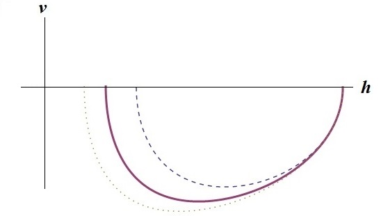
Figure 1: A diagram depicting the behavior of three solutions of the system (2) with same initial conditions. For $c<c_{o}<d$, the solid line corresponds to $h_{c_{o},\sqrt{6}}$, the dashed one to $h_{d,\sqrt{6}}$ and the dotted one to $h_{c,\sqrt{6}}$.

Now, take $s_{1}=s_{2}=\sqrt{6}$, $c<d$ as before, and such that $h_{c}=h_{c,\sqrt{6}}$ and $h_{d}=h_{d,\sqrt{6}}$, both have positive minimums $m_{c}$ and $m_{d}$, respectively. We have their corresponding integral curves $\gamma_{c}$ and $\gamma_{d}$.

Define the function $min:(c,d)\to(0,2)$ which assigns to each $a\in(c,d)$ the first minimum value of the solution $h_{a}^{\sqrt{6}}$.

Claim: The function $min$ is well defined, continuous and increasing.

If $\gamma_{c}$ goes under $\gamma_{d}$, it has to intersect some $\gamma_{d}^{s}$, with $2<s<\sqrt{6}$. But then $\gamma_{c}$ also intersects every integral curve $\gamma_{d}^{t}$, with $t<s$. Take $\gamma_{d}^{\frac{s+\sqrt{6}}{2}}$, for instance. Since $d>c$, by previous discussion, $\gamma_{c}$ stays below $\gamma_{d}^{\frac{s+\sqrt{6}}{2}}$ and cannot intersect $\gamma_{d}^{s}$. Then, in particular $m_{c}<m_{d}$. Same argument applies to each $a\in(c,d)$, the solution $h_{a,\sqrt{6}}$ has a minimum. Then the associated integral curve is closed, since $\sqrt{6}>2$. We have that $m_{d}<min(a)<m_{c}$.

Therefore, it can only exist one $c_{o}\in(c,d)$ such that the solution $h_{c_{o},\sqrt{6}}$ to (2.13) with $h_{c_{o},\sqrt{6}}^{\prime}(0)=0$ has as minimum value $\sqrt{2}$.

Finally, the value of $c_{o}$ can be computed numerically by solving the equation (2.13) for different parameters $c$, and initial conditions $h(0)=\sqrt{6}$ and $h^{\prime}(0)=0$. By the claim, if $c<d$ are two values for which the solutions $h_{c}$ and $h_{d}$ each have minimums $m_{c},m_{d}$, and $m_{d}<\sqrt{2}<m_{c}$ then we know that $c<c_{o}<d$. Then $c_{o}$ can be approximated by interpolation.

Cao also obtained the value of $c_{o}$ as root of the function:

$$k(x)=e^{2x}(2-4x+3x^{2})-2+x^{2}.$$

See Lemma 4.1. in [5]. $\square$

3 Scalar curvature and the Yamabe equation

In this section we will write the Yamabe equation on $\mathbb{CP}^{2}\#\overline{\mathbb{CP}^{2}}$ for a $U(2)-$invariant function. Recall that $\mathbf{g}$ has positive Ricci curvature [5]. We will use this to see that $S_{\mathbf{g}}$ is a decreasing function of $t$ on $S^{3}\times(\alpha,\beta)$. For the sake of completeness we give a proof of the positivity of Ricci curvature using our description of $\mathbf{g}$.

Proposition 3.1

The Koiso- Cao soliton $\mathbf{g}$ has positive Ricci curvature.

Proof:

For a gradient shrinking soliton we have the equation (2.4). Note that since $Hess(u)$ is diagonal in the orthonormal basis $E$, then so is the Ricci curvature of $\mathbf{g}$. Recall also that $\mathbf{g}$ is Kähler, then

$$Ric\left(\frac{X}{f},\frac{X}{f}\right)=Ric(H,H)$$

$$Ric\left(\frac{Z}{h},\frac{Z}{h}\right)=Ric\left(\frac{Y}{h},\frac{Y}{h}\right).$$

Then we only have to show that the functions $Ric(H,H)$ and $Ric(\frac{Y}{h},\frac{Y}{h})$ are positive. Using the Hessian (2) and the expression of $u$ (2.6) we obtain

$$Ric(H,H) = g(H,H)-Hess(u)(H,H)$$

$$= 1-u^{\prime\prime}$$

$$= 1+c(hh^{\prime\prime}+h^{\prime 2}),$$

and

$$Ric\left(\frac{Y}{h},\frac{Y}{h}\right) = g\left(\frac{Y}{h},\frac{Y}{h}\right)-Hess(u)\left(\frac{Y}{h},\frac{Y}{h}\right)$$

$$= 1-\frac{h^{\prime}u^{\prime}}{h}$$

$$= 1+ch^{\prime 2}.$$

First we will lead with the Ricci curvature in the direction of $Y$. From equation (2.13) we rewrite

$$(hh^{\prime\prime}+h^{\prime 2})+h^{\prime 2}-2+\frac{h^{2}}{2}(1+ch^{\prime 2})=0$$

which is the same as:

$$f^{\prime}=h^{\prime 2}-2+\frac{h^{2}}{2}(1+ch^{\prime 2})$$ (3.1)

Let $A(x)=x-2+\frac{b^{2}}{2}(1+cx)$. If we differentiate with respect to $x$,

$$\frac{d}{dx}A=1+c\frac{b^{2}}{2}$$

The critical points of $A$ occurs when $\frac{b^{2}}{2}=-1/c$.

Claim: $1+ch^{\prime 2}>0$.

We have a critical point of the function $(1+ch^{\prime 2})$ if $h^{\prime}=0$ or $h^{\prime\prime}=0$. Observe that that $h^{\prime}=0$ and $h^{\prime\prime}=0$ can not happen simultaneously, else the value of the critical points would be $2$. This is not possible since critical values have to be $\sqrt{2}$ and $\sqrt{6}$. If $h^{\prime}=0$, the claim follows and then $Ric(\frac{Y}{h},\frac{Y}{h})>0$ at $0$ and $\beta$. For those points where $h^{\prime\prime}=0$, from equation (2.13):

$$h^{\prime 2}=\frac{4-h^{2}}{4+ch^{2}}$$ (3.2)

We will considerate two cases.

1. If $3>\frac{h^{2}}{2}\geq-1/c$. Then, $4-h^{2}<4+2/c$. From the value of $c=-0.5276195198969626$ we have $4+2/c<1$. Also, $4+6c<4+ch^{2}$. If follows that

   $$h^{\prime 2}<\frac{4+2/c}{4+6c}<\frac{1}{4+6c}<-1/c,$$

   and then $1+ch^{\prime 2}>0$.

2. If $1<\frac{h^{2}}{2}<-1/c$, we have $4-h^{2}<2$ and $2<4+ch^{2}$. Then:

   $$h^{\prime 2}=\frac{4-h^{2}}{4+ch^{2}}<1$$

   The claim is proved, and then $Ric(\frac{Y}{h},\frac{Y}{h})>0$.

On the other hand, for the Ricci curvature in the direction of $H$, note that, since $-1<c<1$ and $h(0)h^{\prime\prime}(0)=-h(\beta)h^{\prime\prime}(\beta)=1$, $Ric(H,H)$ is positive at $0$ and $\beta$. Then it remains to prove that $1+c(hh^{\prime\prime}+h^{\prime 2})>0$ for every $t\in(0,\beta)$.

Since $c<0$, we have to prove $f^{\prime}=(hh^{\prime\prime}+h^{\prime 2})>1/c\approx-1.8$. It is enough to see $f^{\prime}>-1$. Hence we will show the bound for $f^{\prime}$ in the two previous cases.

Using equation (3.1), the fact that $Ric(\frac{Y}{h},\frac{Y}{h})>0$ and the value of $c$:

1. If $\frac{h^{2}}{2}\geq-1/c$ we have,

   $$f^{\prime} = h^{\prime 2}-2+\frac{h^{2}}{2}(1+ch^{\prime 2})$$

   $$\geq h^{\prime 2}-2-\frac{1}{c}(1+ch^{\prime 2})$$

   $$= -2-1/c>-1$$

2. If $1<\frac{h^{2}}{2}<-1/c$, first note that $(1+\frac{ch^{2}}{2})>0$, and since $1<\frac{h^{2}}{2}$:

   $$f^{\prime} = h^{\prime 2}(1+\frac{ch^{2}}{2})+\frac{h^{2}}{2}-2$$

   $$> \frac{h^{2}}{2}-2>-1$$

Therefore, $f^{\prime}>-1$, and so $Ric(H,H)>0$. $\square$

Let $\psi$ be a smooth function on $S^{3}\times(0,\beta)$ invariant by the action of $U(2)$, then by (2) we get

$$\triangle_{g}\psi = -\frac{f^{\prime}\psi^{\prime}}{f}-2\frac{h^{\prime}\psi^{\prime}}{h}-\psi^{\prime\prime}$$ (3.3)

$$= -\psi^{\prime}\left(\frac{hh^{\prime\prime}+h^{\prime 2}}{hh^{\prime}}+2\frac{h^{\prime}}{h}\right)-\psi^{\prime\prime}$$

$$= -\psi^{\prime}\left(\frac{h^{\prime\prime}}{h^{\prime}}+3\frac{h^{\prime}}{h}\right)-\psi^{\prime\prime}.$$

Then for $u=-\frac{ch^{2}}{2}$ we have:

$$\triangle u = \frac{d}{dt}\left(\frac{ch^{2}}{2}\right)\left(\frac{h^{\prime\prime}}{h^{\prime}}+3\frac{h^{\prime}}{h}\right)+\frac{d^{2}}{dt^{2}}\left(\frac{ch^{2}}{2}\right)$$

$$= chh^{\prime\prime}+3ch^{\prime 2}+chh^{\prime\prime}+ch^{\prime 2}$$

$$= 4ch^{\prime 2}+2chh^{\prime\prime}$$

Now, taking the trace of the soliton equation (2.4) we obtain

$$S-\triangle u=4$$

and therefore the scalar curvature is:

$$S=4ch^{\prime 2}+2chh^{\prime\prime}+4.$$ (3.4)

From Proposition 2.1 and Proposition 2.2 we obtain:

$$S(0) = 4-2c>0$$

$$S(\beta) = 4+2c>0$$ (3.5)

Proposition 3.2

The scalar curvature of the Koiso-Cao soliton is decreasing as a function of $t\in[0,\beta]$.

Proof:

Take the derivative with respect to $t$ of (3.4), then:

$$S^{\prime}=8ch^{\prime}h^{\prime\prime}+2c(hh^{\prime\prime\prime}+h^{\prime}h^{\prime\prime})=10ch^{\prime}h^{\prime\prime}+2chh^{\prime\prime\prime}$$

But,

$$Ric(H,H) = -\frac{f^{\prime\prime}}{f}-2\frac{h^{\prime\prime}}{h}$$

$$= -\frac{hh^{\prime\prime\prime}+5h^{\prime}h^{\prime\prime}}{hh^{\prime}}.$$

Since $Ric(H,H)>0$, we have that $hh^{\prime\prime\prime}+5h^{\prime}h^{\prime\prime}>0$. Therefore, since $c<0$ , $S^{\prime}<0$ on $(0,\beta)$. $\square$

Let $\varphi$ be a smooth function invariant under the action of $U(2)$ on $\mathbb{CP}^{2}\#\overline{\mathbb{CP}^{2}}$. Then we identify $\varphi$ with a function $\phi:[0,\beta]\to\mathbb{R}$ such that $\phi^{\prime}(0)=\phi^{\prime}(\beta)=0$. We use previous calculation of the Laplacian (3.3) to obtain the Yamabe equation of the Koiso-Cao soliton:

$$6\phi^{\prime}\left(\frac{h^{\prime\prime}}{h^{\prime}}+3\frac{h^{\prime}}{h}\right)+6\phi^{\prime\prime}+S_{\mathbf{g}}\phi=\lambda\phi^{3}$$ (3.6)

Since Koiso-Cao soliton has positive scalar curvature, then $\lambda$ has to be positive. We fix $\lambda=1$.

4 Proof of Theorem 1

Let $\phi$ be a positive $U(2)-$invariant function on $S^{3}\times(0,\beta)$ with the Kähler metric $g$. In order to $\phi^{2}\cdot\mathbf{g}$ be a Riemannian metric on $\mathbb{CP}^{2}\#\overline{\mathbb{CP}^{2}}$ , $\phi$ must satisfy $\phi^{\prime}(0)=\phi^{\prime}(\beta)=0$. Additionally, it has constant scalar curvature equals $1$ if $\phi$ satisfies the Yamabe equation (3.6):

$$6\phi^{\prime}\left(\frac{h^{\prime\prime}}{h^{\prime}}+3\frac{h^{\prime}}{h}\right)+6\phi^{\prime\prime}+S_{\mathbf{g}}\phi=\phi^{3}$$

Since:

$$\lim_{t\to 0}\phi^{\prime}\frac{h^{\prime\prime}}{h^{\prime}} = \lim_{t\to 0}\left(\frac{\phi^{\prime}h^{\prime\prime\prime}}{h^{\prime\prime}}+\phi^{\prime\prime}\right)$$

$$= \phi^{\prime\prime}(0)$$

then we have:

$$12\phi^{\prime\prime}(0)=\phi(0)(\phi^{2}(0)-S(0))$$

For $t\in(0,\beta)$ with $\phi^{\prime}(t)=0$,

$$6\phi^{\prime\prime}(t)=\phi(t)(\phi^{2}(t)-S(t)).$$

Claim: $\phi^{2}(0)\leq S(0)=4-2c$ (by (3)).

If $\phi^{2}(0)>S(0)$ then $0$ is a local minimum. $\phi$ increases and $S$ decreases. After $0$, at the next critical point of $\phi$ we would again have that $\phi^{2}>S$ and it would be a minimum.

In particular, same argument says that there is no local minimums on $[0,\beta)$. Therefore, $0$ is a local maximum and $\beta$ a local minimum, and there is no more critical points of $\phi$ on $(0,\beta)$. Then $\phi$ is decreasing.

We have:

$$\sqrt{S(\beta)}\leq\phi(\beta)\leq\phi(0)\leq\sqrt{S(0)}$$

Remember that one $U(2)$-invariant solution to Yamabe equation is guaranteed (see Hebey-Vaugon [11]. It remains to prove uniqueness. If $s\in(\sqrt{S(\beta)},\sqrt{S(0)}]$, let $\phi_{s}$ be a solution to the Yamabe equation (3.6) such that $\phi_{s}(0)=s$. Let $s_{1}$, $s_{2}\in(\sqrt{S(\beta)},\sqrt{S(0)}]$, $s_{1}\textless s_{2}$. We have $0$ is a local maximum for both solutions $\phi_{s_{1}}$ and $\phi_{s_{2}}$. Define $F(t):=\phi_{s_{2}}-\phi_{s_{1}}$.

Claim:  $F$ has a local minimum at $0$.

Note that $F(0)>0$. Since $0$ is a critical point of $\phi_{s_{1}}$ and $\phi_{s_{2}}$, so it is for $F$. Since $\phi_{s_{1}}$ and $\phi_{s_{2}}$ satisfy (3.6), it follows that:

$$F^{\prime\prime}(0)=\frac{1}{12}\left(\phi_{s_{2}}^{3}(0)-\phi_{s_{2}}(0)S(0)-(\phi_{s_{1}}^{3}(0)-\phi_{s_{1}}(0)S(0)\right)$$

Consider the function $v(x)=x^{3}-S(0)x$. Then:

$$v^{\prime}(x)=3x^{2}-S(0)$$

Note that $x_{o}:=\sqrt{\frac{S(0)}{3}}$ is the only critical point, and $v$ is increasing on $(\sqrt{\frac{S(0)}{3}},\sqrt{S(0)})$.

We have, by (3) and the value of $c$,

$$S(0)=4-2c=5.0552\ \ \ \text{and}\ \ \ S(\beta)=4+2c=2.9447$$

then

$$\sqrt{S(0)}=2.2483,\ \ \ \sqrt{S(\beta)}=1.716,\ \ \ \text{and}\ \ \ \sqrt{\frac{S(0)}{3}}=1.2981.$$

Hence, since

$$\sqrt{\frac{S(0)}{3}}\textless\sqrt{S(\beta)}\textless\phi_{s_{1}}(0)\textless\phi_{s_{2}}(0)\leq\sqrt{S(0)},$$

it follows that $F^{\prime\prime}(0)\textgreater 0$, and so $0$ is a local minimum of $F$.

Hence, $F$ is positive and increasing on $(0,\varepsilon)$, for $\varepsilon\textgreater 0$ enough small. Assume that there exists $t_{o}\in(\varepsilon,\beta]$ such that $F^{\prime}(t_{o})=0$, and take the first critical point. The discussion above applies for $t_{o}$, that is, we have:

$$F^{\prime\prime}(t_{o})=\frac{1}{6}\left(\phi_{s_{2}}^{3}(t_{o})-\phi_{s_{2}}(t_{o})S(t_{o})-(\phi_{s_{1}}^{3}(t_{o})-\phi_{s_{1}}(t_{o})S(t_{o})\right)$$

Similarly as before, consider the function $g(x)=x^{3}-S(t_{o})x$. Then $x_{1}:=\sqrt{\frac{S(t_{o})}{3}}$ is its only critical point, which is a minimum. From the choosing of $t_{o}$ it follows :

$$\sqrt{\frac{S(t_{o})}{3}}\textless S(\beta)\textless\phi_{s_{1}}(t_{o})\textless\phi_{s_{2}}(t_{o})$$

Then $t_{o}$ is a local minimum of $F$. But this implies there are another $t_{1}\in(0,t_{o})$ satisfying $F^{\prime}(t_{1})=0$, which is a contradiction, since $t_{o}$ was the first point.

We have proven that $F^{\prime}\textgreater 0$ on $(0,\beta]$ and in particular $F^{\prime}(\beta)=\phi_{s_{2}}(\beta)-\phi_{s_{1}}(\beta)$>0. Then it cannot happen that $\phi_{s_{1}}^{\prime}(\beta)=\phi_{s_{2}}^{\prime}(\beta)=0$. This proves uniqueness.

CIMAT, GUANAJUATO, GTO., México

E-mail address: jonatan@cimat.mx

References

• [1]
• [2] Aubin, T., Équations différentielles non linéaires et problème de Yamabe concernant la courbure scalaire, J. Math. Pures Appl., 55, 269-296, 1976.
• [3] Bergery, L. B., Sur des nouvelles variétés Riemanniennes d’Einstein, Publications de l’Institut Elie Cartan, Nancy, (1982).
• [4] Brendle, S., Blow-up phenomena for the Yamabe equation, Journal Amer. Math. Soc. 21 (2008), 951-979.
• [5] Cao, H.-D., Existence of gradient Kähler-Ricci solitons, Elliptic and Parabolic Methods in Geometry (Minneapolis, MN, 1994), A. K. Peters, Wellesley, MA, (1996) 1-16.
• [6] Cao, H.-D, Recent progress on Ricci solitons, Recent advances in geometric analysis, Adv. Lect. Math. (ALM), vol. 11, Int. Press, Somerville, MA, 2010, pp. 1-38.
• [7] Chow, B.; Knopf D., The Ricci Flow: An Introduction, AMS Math. Surveys and Monographs, 2004.
• [8] Dancer, A. S.; Wang, M. Y., On Ricci solitons of cohomogeneity one, Ann. Glob. Anal. Geom. (2011) 39:259-292.
• [9] Dancer, A. S.; Hall, Stuart J.; Wang, M. Y., Cohomogeneity one shrinking Ricci solitons: An analytic and numerical study., Asian J. Math. 17 (2013), no. 1, 33–62.
• [10] Hamilton, R. S., The formation of singularities in the Ricci flow, Surveys in Differential Geometry (Cambridge, MA, 1993), 2, 7-136, International Press, Combridge, MA, 1995.
• [11] Hebey, E., Vaugon, M., Le problème de Yamabe équivariant, Bull. Sci. Math. 117 (1993), 241-286.
• [12] Henry, G.; Petean, J., Isoparametric hypersurfaces and metrics of constant scalar curvature, The Asian Journal of Mathematics, (2014) Vol. 18 1:53-68.
• [13] Ivey, T., Ricci solitons on compact three-manifolds, Diff. Geom. Appl. 3(1993), 301-307.
• [14] Koda, T., A remark on the manifold $\mathbb{CP}^{2}\#\overline{\mathbb{CP}^{2}}$ with Bérard Bergery’s metric, Annals of Global Analysis and Geometry 11: 323-329, 1993.
• [15] Koiso, N., On rotationally symmetric Hamilton’s equation for Kähler-Einstein metrics, Adv. Studies Pure Math., 18-I, Academic Press, (1990), 327-337.
• [16] Lee, J. M. and Parker, T.H., The Yamabe Problem, Bull. Amer. Math. Soc., 17, 37-91, 1987.
• [17] de Lima, L.L., Piccione, P., Zedda, M., On bifurcation of solutions of the Yamabe problem in product manifolds Ann. Inst. H. Poincaré Anal. Non Linéaire 29, No. 2, 261-277 (2012).
• [18] Obata, M., The conjectures on conformal transformations of Riemannian manifolds, J. Diff.Geom., 6 (1971), 247-258.
• [19] Perelman, G., The entropy formula for the Ricci flow and its geometric applications, arXiv:math.DG/0211159.
• [20] Petean, J., Metrics of Constant Scalar Curvature Conformal to Riemannian Products, Proceedings of the American Mathematical Society, 138, 8, 2897-2905, (2010).
• [21] Pollack, D., Nonuniqueness and high enegergy solutions for a conformally invariant scalar equation, Comm. Anal. Geom. 1 (1993), 347-414.
• [22] Schoen, R., Conformal deformation of a Riemannian metric to constant scalar curvature, J. Differential Geom., 20, 479-495, 1984.
• [23] Trudinger, N. S., Remarks concerning the conformal deformation of Riemannian structures on compact manifolds, Ann. Scuola Norm. Sup. Pisa, 22, 265-274, 1968.
• [24] Wang, Xu-Jia; Zhu, Xiaohua, Kähler-Ricci solitons on toric manifolds with positive first Chern class. Adv. Math. 188 (2004), no. 1, 87-103.
• [25] Yamabe, H., On a deformation of Riemannian structures on compact manifolds, Osaka Math. J., 12, 21-37, 1960.