Modeling real phononic crystals via the weighted relaxed micromorphic model with free and gradient micro-inertia

Abstract

In this paper the relaxed micromorphic continuum model with weighted free and gradient micro-inertia is used to describe the dynamical behavior of a real two-dimensional phononic crystal for a wide range of wavelengths. In particular, a periodic structure with specific micro-structural topology and mechanical properties, capable of opening a phononic band-gap, is chosen with the criterion of showing a low degree of anisotropy (the band-gap is almost independent of the direction of propagation of the traveling wave). A Bloch wave analysis is performed to obtain the dispersion curves and the corresponding vibrational modes of the periodic structure. A linear-elastic, isotropic, relaxed micromorphic model including both a free micro-inertia (related to free vibrations of the microstructures) and a gradient micro-inertia (related to the motions of the microstructure which are coupled to the macro-deformation of the unit cell) is introduced and particularized to the case of plane wave propagation. The parameters of the relaxed model, which are independent of frequency, are then calibrated on the dispersion curves of the phononic crystal showing an excellent agreement in terms of both dispersion curves and vibrational modes. Almost all the homogenized elastic parameters of the relaxed micromorphic model result to be determined. This opens the way to the design of morphologically complex meta-structures which make use of the chosen phononic structure as the basic building block and which preserve its ability of “stopping” elastic wave propagation at the scale of the structure.

Keywords: microstructure, metamaterials, phononic crystals, relaxed micromorphic model, gradient micro-inertia, free micro-inertia, complete band-gaps, fitting of the elastic coefficients, inverse approach

AMS 2010 subject classification: 74A10 (stress), 74A30 (non-simple materials), 74A60 (micro-mechanical theories), 74E15 (crystalline structure), 74M25 (micro-mechanics), 74Q15 (effective constitutive equations)

1 Introduction

A new class of innovative engineered materials, also known as phononic/photonic crystals or metamaterials, showing exotic behaviours with respect to both mechanical and electromagnetic wave propagation are recently attracting great interest for their unique unconventional properties, such as frequency band gaps [1, 33, 47], negative refraction [37, 41], cloaking [12, 42], filtering/focusing capabilities [9], etc. Among these unorthodox properties, the ability to “stop” or “bend” the propagation of waves of light or sound with no energetic inputs is the main aspect disclosing rapid and previously unimaginable technological advancements.

Specifically, in the electromagnetic domain, these metamaterials might be used for rendering aircrafts or other vehicles undetectable to radar, for making objects invisible to the human eye [42], or to realize the so-called super-lenses that would allow the human eye to see single viruses or nano-organisms [13]. Other important applications concern the revolution of the electronics in communication and information management systems, using light instead of electrons as the information carrier, through photonic band-gap materials [5]. Finally, in order to obtain wider and frequency tunable band-gaps several approaches have been proposed by varying the properties of the materials as well as their spatial ordered/disordered arrangement [18, 17, 20, 32, 23, 48].

Notwithstanding the interest raised by such “electromagnetic metamaterials”, they will not make the object of the present paper which will be instead centered on the study of “mechanical metamaterials”.

As far as phononic crystals and mechanical metamaterials are concerned, regrettably, their introduction into the current technology appears less advanced, although many potential applications of practical implementation have already been proposed: from seismic protection [11, 34] to environmental noise reduction[33, 36], from sub-wavelength imaging to focusing[4], acoustic cloaking [35] and even thermal control[31].

Such materials also pushed innovative naval, automotive and aeronautical vehicles conception in view of absorbing external solicitations and shocks, thereby drastically improving their internal comfort. What’s more, civil engineering structures which are built in the vicinity of sources of vibrations such as metro lines, tramways, train stations, and so forth would take advantage of the use of these metamaterials to ameliorate the enjoyment of internal and external environments [21].

Based on the same principle, passive engineering devices perfectly able to insulate from noise [22] could be easily conceived and produced at relatively low costs. The conception of waveguides used to optimize energy transfers by collecting waves in slabs [46] or wires, as well as the design of wave screens employed to protect from any sort of mechanical wave could also see a new technological revolution. And many other unprecedented applications that, at this juncture, we cannot even envision could be abruptly disclosed once such metamaterials would become easily accessible.

In this paper, we focus our attention on those metamaterials which are able to “stop” wave propagation, i.e. metamaterials in which waves within precise frequency ranges cannot propagate. Such frequency intervals at which wave inhibition occurs are known as frequency band-gaps and their intrinsic characteristics (characteristic values of the gap frequency, extension of the band-gap, etc.) strongly depend on the metamaterial microstructure.

The approach that we use here to describe the mechanical behavior of band-gap metamaterials is in complete rupture to the classical approaches that are nowadays used to study phononic crystals. Indeed, the most spread approach to the modeling of band-gap metamaterials is that of starting from a precise microstructure and to derive the dispersive properties of the equivalent medium using upscaling arguments or numerical homogenization techniques (see e.g. [24, 43, 45, 44, 2, 6, 7, 8]). If such methods allow, on the one hand, to make a direct comparison between the micro and the macro properties, on the other hand, they are often strongly limited to large wavelengths.

From a different perspective, we start from a macroscopic (directly defined at the homogenized level) linear-elastic relaxed micromorphic model (which is known to be able to describe band-gap behaviors and to be well-posed [14, 28, 29, 27, 25, 30, 39, 40]) and we determine the parameters of our model on real metamaterials by an inverse approach. Similarly to classical isotropic linear-elasticity where two parameters (Young modulus and Poisson ratio) are needed to describe the average behavior of a large class of engineering materials, in the same way in isotropic, linear-elastic enriched elasticity few extra parameters will be needed to describe the averaged behavior of a relatively huge class of metamaterials sharing the common characteristic property of stopping wave propagation. Such parameters, being constitutive parameters, do not depend on frequency as it is instead usually the case when dealing with homogenized media arising from classical homogenization techniques.

The fact of determining the coefficients of an enriched continuum model on real band-gap metamaterials with given microstructure is of paramount importance for the subsequent implementation of the model in Finite Element codes and for an effective design of morphologically complex band-gap metastructures.

1.1 Notations

In this contribution, we denote by $\mathbb{R}^{3\times 3}$ the set of real $3\times 3$ second order tensors, written with capital letters. We denote respectively by $\cdot\>$, $:$ and $\left.\langle\cdot,\cdot\right.\rangle$ a simple and double contraction and the scalar product between two tensors of any suitable order. Everywhere we adopt the Einstein convention of sum over repeated indices if not differently specified. The standard Euclidean scalar product on $\mathbb{R}^{3\times 3}$ is given by $\langle{X},{Y}\rangle_{\mathbb{R}^{3\times 3}}=\,\mathrm{tr}({X\cdot Y^{T}})$, and thus the Frobenius tensor norm is $\|{X}\|^{2}=\langle{X},{X}\rangle_{\mathbb{R}^{3\times 3}}$. In the following we omit the index $\mathbb{R}^{3},\mathbb{R}^{3\times 3}$ if no confusion can arise. The identity tensor on $\mathbb{R}^{3\times 3}$ will be denoted by $\,\mathds{1}$, so that $\,\mathrm{tr}({X})=\langle{X},{\,\mathds{1}}\rangle$.

We consider a body which occupies a bounded open set $B$ of the three-dimensional Euclidian space $\mathbb{R}^{3}$ and assume that its boundary $\partial B$ is a smooth surface of class $C^{2}$. An elastic material fills the domain $B\subset\mathbb{R}^{3}$ and we refer the motion of the body to rectangular axes $Ox_{i}$.

For vector fields $v$ with components in ${\rm H}^{1}(B)$, i.e. $v=\left(v_{1},v_{2},v_{3}\right)^{T}\,,v_{i}\in{\rm H}^{1}(B),$ we define $\nabla\,v=\left((\nabla\,v_{1})^{T},(\nabla\,v_{2})^{T},(\nabla\,v_{3})^{T}\right)^{T}$, while for tensor fields $P$ with rows in ${\rm H}({\rm curl}\,;B)$, resp. ${\rm H}({\rm div}\,;B)$, i.e. $P=\left(P_{1}^{T},P_{2}^{T},P_{3}^{T}\right)$, $P_{i}\in{\rm H}({\rm curl}\,;B)$ resp. $P_{i}\in{\rm H}({\rm div}\,;B)$ we define ${\rm Curl}\,P=\left(({\rm curl}\,P_{1})^{T},({\rm curl}\,P_{2})^{T},({\rm curl}\,P_{3})^{T}\right)^{T},$ ${\rm Div}\,P=\left({\rm div}\,P_{1},{\rm div}\,P_{2},{\rm div}\,P_{3}\right)^{T}.$

As for the kinematics of the considered micromorphic continua, we introduce the functions

$$\chi(X,t):B\subset\mathbb{R}^{3}\rightarrow\mathbb{R}^{3},\qquad\qquad P(X,t):B\subset\mathbb{R}^{3}\rightarrow\mathbb{R}^{3\times 3},$$

which are known as placement vector field and micro-distortion tensor, respectively. The physical meaning of the placement field is that of locating, at any instant $t$, the current position of the material particle $X\in B$, while the micro-distortion field describes deformations of the microstructure embedded in the material particle $X$. As it is usual in continuum mechanics, the displacement field can also be introduced as the function $u(X,t):B\subset\mathbb{R}^{3}\rightarrow\mathbb{R}^{3}$ defined as

$$u(X,t)=\chi(X,t)-X.$$

2 The relaxed micromorphic model with weighted free and gradient micro inertia

In recent previous contributions [14, 19, 28, 29, 27, 39, 40], the relaxed micromorphic model has been introduced as that enriched model of the micromorphic type which, in the linear-elastic, isotropic case, features a strain energy density of the form

$$W= \underbrace{\mu_{e}\,\lVert\,\mathrm{sym}\,\left(\,\nabla u\,-{P}\right)\rVert^{2}+\frac{\lambda_{e}}{2}\left(\mathrm{tr}\left(\,\nabla u\,-{P}\right)\right)^{2}}_{\mathrm{{\textstyle isotropic\ elastic-energy}}}+\underbrace{\mu_{c}\,\lVert\,\mathrm{skew}\left(\,\nabla u\,-{P}\right)\rVert^{2}}_{\mathrm{{\textstyle rotational\ elastic\ coupling}}}$$ (1)

$$\quad+\underbrace{\mu_{\mathrm{micro}}\,\lVert\,\mathrm{sym}\,{P}\rVert^{2}+\frac{\lambda_{\mathrm{micro}}}{2}\,\left(\mathrm{tr}{P}\right)^{2}}_{\mathrm{{\textstyle micro-self-energy}}}+\underbrace{\frac{\mu_{e}L_{c}^{2}}{2}\,\lVert\,\mathrm{Curl}{P}\rVert^{2}}_{\mathrm{{\textstyle isotropic\ curvature}}}\,,$$

where all the introduced constitutive coefficients are positive constant (the Cosserat couple modulus $\mu_{c}$ can also be vanishing in some special cases without affecting the well-posedness of the model (see [38]). This particular constitutive form of the strain energy density will be used in the present paper as descriptive of a certain class of metamaterials with particular topologies that will be shown to exhibit band-gap behaviors. Such constitutive choice is dictated by the previous works on this subject [28, 29, 27, 30, 26] showing that the relaxed micromorphic model is the most effective enriched continuum model that can be used for the simultaneous description of band-gaps and non-localities in metamaterials. As we will show in the second part of the paper, the fitting of the parameters on the basis of the dispersion curves, as presented in the present work allows to have a first estimate of the elastic parameters of the relaxed micromorphic model. On the other hand, a fitting procedure based on the dispersion curves alone is not precise enough to allow an accurate estimation of the characteristic length of the considered metamaterial. In this paper, only the main elastic parameters of the model will be then determined, while the effect and associated estimate of the characteristic length will be analyzed in further works where the fitting will be based on the use of the transmission coefficient as done already in [25].

As far as the adopted kinetic energy is concerned, we consider (as done in [14]) a Cartan-Lie decomposition of the free micro-inertia $\left\|{P}_{,t}\right\|^{2}$, as well as of the gradient micro-inertia $\left\|\,\nabla u\,_{,t}\right\|^{2}$ (as presented in [26]). The kinetic energy density that we thus retain in this paper to model the mechanical behavior of the targeted real phononic crystals takes the following form:

$$J=\underbrace{\frac{1}{2}\rho\left\|u_{,t}\right\|^{2}}_{\text{Cauchy inertia}}+\hskip 2.84544pt\underbrace{\frac{1}{2}\eta_{1}\left\|\,\mathrm{dev}\,\mathrm{sym}\,{P}_{,t}\right\|^{2}+\frac{1}{2}\eta_{2}\left\|\,\mathrm{skew}{P}_{,t}\right\|^{2}+\frac{1}{6}\eta_{3}\,\mathrm{tr}\left({P}_{,t}\right)^{2}}_{\text{weighted free micro-inertia}},$$

$$+\hskip 2.84544pt\underbrace{\frac{1}{2}\overline{\eta}_{1}\left\|\,\mathrm{dev}\,\mathrm{sym}\,\,\nabla u\,_{,t}\right\|^{2}+\frac{1}{2}\overline{\eta}_{2}\left\|\,\mathrm{skew}\,\nabla u\,_{,t}\right\|^{2}+\frac{1}{6}\overline{\eta}_{3}\,\mathrm{tr}\left(\,\nabla u\,_{,t}\right)^{2}}_{\text{weighted gradient micro-inertia}},$$

We discuss here briefly the inertia terms appearing in Eq. (LABEL:eq:Kinetic) in order to give an explanation of the adopted nomenclature as well as a general interpretation of the respective physical meaning associated to each term:

• The Cauchy inertia term $\frac{1}{2}\rho\left\|u_{,t}\right\|^{2}$ is the macroscopic inertia introduced in classical linear elasticity. It allows to describe the vibrations associated to the macroscopic displacement field. In an enriched continuum mechanical modeling framework, this means that such terms account for the inertia to vibration of the unit cells considered as material points (or Representative Volume Elements) with apparent mass density $\rho$.

• The term $\frac{1}{2}\eta\left\|{P}_{,t}\right\|^{2}$ accounts for the inertia of the microstructure alone: we called $\eta$ free micro-inertia [26] since it represents the inertia of the microstructure seen as a micro-system whose vibration can be independent of the vibration of the unit cells. An inertia term of this type is mandatory whenever one considers an enriched model of the micromorphic type, i.e. a model that features an enriched kinematics $(u,P)$. Indeed, it would be senseless to introduce an enriched kinematics, an enriched constitutive form for the strain energy density and then avoid to introduce this free micro-inertia in the model. It would be like introducing a complex constitutive structure to describe in detail the mechanical behavior of microstructured materials while not giving to the model the possibility of activating the vibrations of such microstructures. The free micro-inertia allows us to account for the vibrations of the microstructures that typically appear for high frequencies (i.e. small wavelengths comparable with the characteristic size of the microstructure) in a huge variety of mechanical metamaterials. As we will show in more detail in the remainder of this paper, the Cartan-Lie decomposition of the tensor $P_{,t}$ in its $\,\mathrm{dev}\,\mathrm{sym}\,$ (trace-free symmetric-), $\,\mathrm{skew}$ (skew-symmetric-) and $\,\mathrm{tr}$ (trace-) part allows for the independent control of the cut-off frequencies of the optic branches. This feature will be crucial for the fitting of the parameters of our model on the real metamaterials targeted in this paper.

• The gradient micro-inertia term is of the type $\bar{\eta}\left\|\,\nabla u\,_{,t}\right\|^{2}$ and, when split using a Cartan-Lie decomposition, it takes the form shown in Eq. (LABEL:eq:Kinetic) (see also [26]). Such term allows to account for some specific vibrations of the microstructure which are directly coupled to the deformation of the unit cell at the macro scale. In other words, this term allows to account for the inertia of the motions of the microstructure which are generated as a consequence of the deformation of the unit cell as a whole. This gradient micro-inertia term brings additional informations with respect to the free micro-inertia term previously described and this fact is translated on the behavior of some dispersion curves that, as we will see, can be flattened when increasing the value of $\bar{\eta}_{1}$, $\bar{\eta}_{2}$ or $\bar{\eta}_{3}$.

The action functional $\mathcal{A}$ of the considered model can be introduced as

$$\mathcal{A}=\int_{0}^{T}\int_{B_{L}}(J-W)\,dv\,dt,$$ (3)

where $[0,T]$ is the interval of time during which the motion of the considered micromorphic system wants to be observed. Following standard variational arguments, the equations of motion of the system can be obtained by making the action functional (3) stationary and take the form (see also [19, 39, 40, 28, 29])

$$\rho\,u_{,tt}-\mathrm{Div}[\,\mathcal{I}\,] =\mathrm{Div}\left[\,2\,\mu_{e}\,\,\mathrm{sym}\,\left(\,\nabla u\,-{P}\right)+\lambda_{e}\,\,\mathrm{tr}\left(\,\nabla u\,-{P}\right)\,\mathds{1}+2\,\mu_{c}\,\,\mathrm{skew}\left(\,\nabla u\,-{P}\right)\,\right],$$

$$\eta_{1}\,\,\mathrm{dev}\,\mathrm{sym}\,\,{P}_{,tt} =2\,\mu_{e}\,\,\mathrm{dev}\,\mathrm{sym}\,\,\left(\nabla u-P\right)-2\,\mu_{\mathrm{micro}}\,\mathrm{dev}\,\mathrm{sym}\,\,P-\mu_{e}L_{c}^{2}\,\,\mathrm{dev}\,\mathrm{sym}\,\left(\,\mathrm{Curl}\,\,\mathrm{Curl}\,P\right),$$

$$\eta_{2}\,\mathrm{skew}\,{P}_{,tt} =2\,\mu_{c}\,\mathrm{skew}\,\left(\nabla u-P\right)-\mu_{e}L_{c}^{2}\,\,\mathrm{skew}\left(\,\mathrm{Curl}\,\,\mathrm{Curl}\,P\right)$$

$$\frac{1}{3}\eta_{3}\,\mathrm{tr}{P}_{,tt} =\left(\frac{2}{3}\mu_{e}+\lambda_{e}\right)\,\mathrm{tr}\left(\nabla u-P\right)-\left(\frac{2}{3}\mu_{\mathrm{micro}}+\lambda_{\mathrm{micro}}\right)\,\mathrm{tr}{P}-\frac{1}{3}\mu_{e}L_{c}^{2}\,\mathrm{tr}\left(\,\mathrm{Curl}\,\,\mathrm{Curl}\,P\right).$$ (4)

where, for compactness, we set $\mathcal{I}=\overline{\eta}_{1}\,\,\mathrm{dev}\,\mathrm{sym}\,\,\nabla u\,_{,tt}+\overline{\eta}_{2}\,\,\mathrm{skew}\,\nabla u\,_{,tt}+\frac{1}{3}\overline{\eta}_{3}\,\mathrm{tr}\left(\,\nabla u\,_{,tt}\right)$.

2.1 Plane wave ansatz

We rapidly recall in this subsection how, starting from the equations of motion in strong form for the relaxed micromorphic medium, it is possible to obtain the associated dispersion curves by following standard techniques. We start by making a plane-wave ansatz which means that we assume that all the 12 scalar components of the unknown fields $u(x,t)$ and $P(x,t)$ only depend on the component $x_{1}$ of the space variable $x$ which is also assumed to be the direction of the traveling wave. With this unique assumption, together with the introduction of the new variables

$${P}^{S} :=\frac{1}{3}\,\mathrm{tr}\left({P}\right), {P}_{\left[ij\right]} :=\left(\,\mathrm{skew}{P}\right)_{ij}=\frac{1}{2}\left({P}_{ij}-{P}_{ji}\right),$$ (5)

$${P}^{D} :={P}_{11}-{P}^{S}, {P}_{\left(ij\right)} :=\left(\,\mathrm{sym}\,{P}\right)_{ij}=\frac{1}{2}\left({P}_{ij}+{P}_{ji}\right),$$

$$P^{V} :=P_{22}-P_{33}, i,j=\{1,2,3\},$$

the equations of motions (4) can be simplified and rewritten, after suitable manipulation, as (see [14, 28, 29, 27] for additional details):

• a set of three equations only involving longitudinal quantities:

  $$\rho\,\ddot{u}_{1}-\frac{2\,\overline{\eta}_{1}+\overline{\eta}_{3}}{3}\,\ddot{u}_{1,11} =\left(2\,\mu_{e}+\lambda_{e}\right)u_{1,11}-2\mu_{e}\,P_{,1}^{D}-(2\mu_{e}+3\lambda_{e})\,P_{,1}^{S}\,,\vspace{0.4cm}$$

  $$\eta_{1}\,\ddot{P}^{D} =\frac{4}{3}\,\mu_{e}\,u_{1,1}+\frac{1}{3}\,\mu_{e}L_{c}^{2}\,P_{,11}^{D}-\frac{2}{3}\,\mu_{e}L_{c}^{2}P_{,11}^{S}-2\left(\mu_{e}+\mu_{\mathrm{micro}}\right)\,P^{D}\,,\vspace{0.4cm}$$ (6)

  $$\eta_{3}\,\ddot{P}^{S} =\frac{2\,\mu_{e}+3\,\lambda_{e}}{3}\,u_{1,1}-\frac{1}{3}\,\mu_{e}L_{c}^{2}P_{,11}^{D}+\frac{2}{3}\,\mu_{e}L_{c}^{2}P_{,11}^{S}$$

  $$\quad-\left(2\,\mu_{e}+3\,\lambda_{e}+2\,\mu_{\mathrm{micro}}+3\,\lambda_{\mathrm{micro}}\right)\,P^{S}\,,$$

• two sets of three equations only involving transverse quantities in the $\xi$-th direction, with $\xi=2,3$:

  $$\rho\,\ddot{u}_{\xi}-\frac{\,\overline{\eta}_{1}+\overline{\eta}_{2}}{2}\,\ddot{u}_{\xi,11} =\left(\mu_{e}+\mu_{c}\right)u_{\xi,11}-2\,\mu_{e}\,P_{\left(1\xi\right),1}+2\,\mu_{c}\,P_{\left[1\xi\right],1},\vspace{0.4cm}$$

  $$\eta_{1}\,\ddot{P}_{\left(1\xi\right)} =\mu_{e}\,u_{\xi,1}+\frac{1}{2}\,\mu_{e}L_{c}^{2}\,P_{(1\xi)}{}_{,11}+\frac{1}{2}\,\mu_{e}L_{c}^{2}\,P_{\left[1\xi\right],11}$$ (7)

  $$\quad-2\left(\mu_{e}+\mu_{\mathrm{micro}}\right)\,P_{(1\xi)},\vspace{0.4cm}$$

  $$\eta_{2}\,\ddot{P}_{\left[1\xi\right]} =-\mu_{c}\,u_{\xi,1}+\frac{1}{2}\,\mu_{e}L_{c}^{2}\,P_{(1\xi),11}+\frac{1}{2}\,\mu_{e}L_{c}^{2}P_{\left[1\xi\right]}{}_{,11}-2\,\mu_{c}\,P_{\left[1\xi\right]},$$

• one equation only involving the variable $P_{\left(23\right)}$:

  $$\eta_{1}\,\ddot{P}_{\left(23\right)}=-2\left(\mu_{e}+\mu_{\mathrm{micro}}\right)P_{\left(23\right)}+\mu_{e}L_{c}^{2}P_{\left(23\right),11},$$ (8)

• one equation only involving the variable $P_{\left[23\right]}$ :

  $$\eta_{2}\,\ddot{P}_{\left[23\right]}=-2\,\mu_{c}\,P_{\left[23\right]}+\mu_{e}L_{c}^{2}P_{\left[23\right],11},$$

• one equation only involving the variable $P^{V}$:

  $$\eta_{1}\,\ddot{P}^{V}=-2\left(\mu_{e}+\mu_{\mathrm{micro}}\right)P^{V}+\mu_{e}L_{c}^{2}P_{,11}^{V}.$$ (9)

Once that this simplified form of the equations of motion is obtained, we look for a wave form solution of the type

$$v_{1}=\beta_{1}\,e^{i(kx_{1}-\omega t)},\qquad v_{2}=\beta_{2}\,e^{i(kx_{1}-\omega t)},\qquad v_{3}=\beta_{3}\,e^{i(kx_{1}-\omega t)},$$

$$v_{4}=\beta_{4}\,e^{i(kx_{1}-\omega t)},\qquad v_{5}=\beta_{5}\,e^{i(kx_{1}-\omega t)},\qquad v_{6}=\beta_{6}\,e^{i(kx_{1}-\omega t)},$$

where $\beta_{1}$, $\beta_{2}$, $\beta_{3}\in\mathbb{C}^{3}$ and $\beta_{4}$, $\beta_{5}$, $\beta_{6}\in\mathbb{C}$ are the unknown amplitudes of the considered waves, $\omega$ is the frequency, $k$ the wavenumber and where, for compactness of notation, we set

$$v_{1}:=\left(u_{1},P_{11}^{D},P^{S}\right),\qquad v_{2}:=\left(u_{2},P_{(12)},P_{[12]}\right),\qquad v_{3}:=\left(u_{3},P_{(13)},P_{[13]}\right),$$

$$v_{4}:=P_{\left(23\right)},\qquad v_{5}:=P_{[23]},\qquad v_{6}:=P^{V}.$$

Replacing the wave-form (LABEL:eq:WaveForm)-(LABEL:eq:Unknowns) in the equations of motion (6)-(9) and simplifying, we end up with the following systems of algebraic equations

$$A_{1}(\omega,k)\cdot\beta_{1}=0,\qquad\qquad A_{\tau}(\omega,k)\cdot\beta_{\tau}=0,\quad\tau=2,3,\qquad\qquad A_{4}(\omega,k)\cdot\alpha=0,$$ (12)

where we set $\alpha=\left(\beta_{4},\beta_{5},\beta_{6}\right)$ and

$$A_{1}(\omega,k)\, =\left(\begin{array}[]{ccc}-\omega^{2}\left(1+k^{2}\,\frac{2\,\overline{\eta}_{1}+\overline{\eta}_{3}}{3\,\rho}\right)+c_{p}^{2}\,k^{2}&\,i\>k\,2\,\mu_{e}/\rho&i\>k\>\left(2\,\mu_{e}+3\,\lambda_{e}\right)/\rho\\ \\ -i\>k\,\frac{4}{3}\,\mu_{e}/\eta_{1}&-\omega^{2}+\frac{1}{3}k^{2}c_{m1}^{2}+\omega_{s}^{2}&-\frac{2}{3}\,k^{2}c_{m1}^{2}\\ \\ -\frac{1}{3}\,i\,k\>\left(2\,\mu_{e}+3\,\lambda_{e}\right)/\eta_{3}&-\frac{1}{3}\,k^{2}\,c_{m3}^{2}&-\omega^{2}+\frac{2}{3}\,k^{2}\,c_{m3}^{2}+\omega_{p}^{2}\end{array}\right),$$ (18)

$$A_{2}(\omega,k)=A_{3}(\omega,k)\, =\left(\begin{array}[]{ccc}-\omega^{2}\left(1+k^{2}\,\frac{\overline{\eta}_{1}+\overline{\eta}_{2}}{2\,\rho}\right)+k^{2}c_{s}^{2}&\,i\,k\,2\,\mu_{e}/\rho&-i\,\frac{\eta_{2}}{\rho}\,\omega_{r}^{2}k\,,\\ \\ -\,i\,k\,\mu_{e}/\eta_{1},&-\omega^{2}+\frac{1}{2}\,c_{m1}^{2}\,k^{2}+\omega_{s}^{2}&\frac{1}{2}\,c_{m1}^{2}\,k^{2}\\ \\ \frac{1}{2}\,i\,\omega_{r}^{2}\,k&\frac{1}{2}\,c_{m2}^{2}\,k^{2}&-\omega^{2}+\frac{1\,}{2}c_{m2}^{2}\,k^{2}+\omega_{r}^{2}\end{array}\right),$$ (24)

$$A_{4}(\omega,k)\, =\left(\begin{array}[]{ccc}-\omega^{2}+c_{m1}^{2}\,k^{2}+\omega_{s}^{2}&0&0\\ \\ 0&-\omega^{2}+c_{m2}^{2}\,k^{2}+\omega_{r}^{2}&0\\ \\ 0&0&-\omega^{2}+c_{m1}^{2}\,k^{2}+\omega_{s}^{2}\end{array}\right).$$ (31)

In the definition of the matrices $A_{i}$, $i=\{1,2,3,4\}$ the following characteristic quantities have also been introduced:

$$\omega_{s} =\sqrt{\frac{2\,(\mu_{e}+\mu_{\mathrm{micro}})}{\eta_{1}}},\qquad\omega_{r}=\sqrt{\frac{2\,\mu_{c}}{\eta_{2}}},\qquad\omega_{p}=\sqrt{\frac{(3\,\lambda_{e}+2\,\mu_{e})+(3\,\lambda_{\mathrm{micro}}+2\,\mu_{\mathrm{micro}})}{\eta_{3}}},\vspace{1.2mm}$$

$$c_{m1} =\sqrt{\frac{\mu_{e}\,L_{c}^{2}}{\eta_{1}}},\qquad c_{m2}=\sqrt{\frac{\mu_{e}\,L_{c}^{2}}{\eta_{2}}},\qquad c_{m3}=\sqrt{\frac{\mu_{e}\,L_{c}^{2}}{\eta_{3}}}\qquad\ \ c_{p}=\sqrt{\frac{\lambda_{e}+2\mu_{e}}{\rho}},\qquad c_{s}=\sqrt{\frac{\mu_{e}+\mu_{c}}{\rho}}.$$

The dispersion curves for the weighted relaxed micromorphic model with free and gradient micro-inertia can hence be obtained as the solutions $\omega=\omega(k)$ of the algebraic equations

$$\underbrace{\mathrm{det}\,A_{1}(\omega,k)=0,}_{\text{longitudinal}}\qquad\qquad\underbrace{\mathrm{det}\,A_{2}(\omega,k)=\mathrm{det}\,A_{3}(\omega,k)=0,}_{\text{transverse}}\qquad\qquad\underbrace{\mathrm{det}\,A_{4}(\omega,k)=0.}_{\text{uncoupled}}$$ (33)

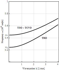
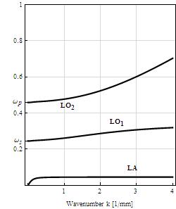
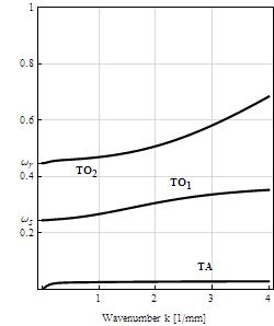
Figure 1: Characteristic dispersion curves of the weighted relaxed micromorphic model obtained with the tentative values of the parameters shown in Tab. 1.

We show in Fig. 1 the characteristic dispersion curves that can be obtained via the weighted relaxed micromorphic model. In such figures the following acronymshave been used accordingly to the preceding papers on this subject:

• TRO: transverse rotational optic,

• TSO: transverse shear optic,

• TCVO: transverse constant-volume optic,

• LA: longitudinal acoustic,

• LO₁-LO₂: $1^{st}$ and $2^{nd}$ longitudinal optic,

• TA: transverse acoustic,

• TO₁-TO₂: $1^{st}$ and $2^{nd}$ transverse optic.

To draw the curves in Fig. 1, we chose the tentative values of the characteristic parameters shown in table 1. From the observation of such curves many features which are important for the subsequent fitting of the parameters can be identified:

• The first main characteristic of the relaxed micromorphic model is that the longitudinal and transverse acoustic waves have an horizontal asymptote which has been seen to be essential for the description of band-gaps in enriched continua [14, 28, 29, 27, 30]. Moreover, it has been shown in [14] that the slopes (close to the origin) of the longitudinal and transverse acoustic curves can be expressed in terms of the parameters of the relaxed model as

  $$\sqrt{\frac{3\,\lambda_{e}\,\lambda_{\mathrm{micro}}\,(\mu_{e}+\mu_{\mathrm{micro}})+2\mu_{e}\,\mu_{\mathrm{micro}}\left[3(\lambda_{e}+\lambda_{\mathrm{micro}})+2(\mu_{e}+\mu_{\mathrm{micro}})\right]+2\lambda_{\mathrm{micro}}\,\mu_{e}^{2}+2\lambda_{e}\,\mu_{\mathrm{micro}}^{2}}{\rho\,(\mu_{e}+\mu_{\mathrm{micro}})\left(3(\lambda_{e}+\lambda_{\mathrm{micro}})+2(\mu_{e}+\mu_{\mathrm{micro}})\right)}},$$

  $$\sqrt{\frac{\mu_{e}\,\mu_{\mathrm{micro}}}{\rho\,(\mu_{e}+\mu_{\mathrm{micro}})}}.$$

  The slope of the longitudinal and transverse acoustic curves will be seen to be a primordial feature for the fitting of the relaxed micromorphic model on real metamaterials. Moreover, such slopes provide a way to compare the relaxed micromorphic model to classical Cauchy elasticity for low frequencies (high wavelengths), since they are a measure of the apparent macroscopic stiffnesses of the considered metamaterial. As a matter of fact, it has been shown in [3] that, using simple homogenization arguments, if one sets

  $$\mu_{\mathrm{macro}}=\frac{\mu_{e}\mu_{\mathrm{micro}}}{\mu_{e}+\mu_{\mathrm{micro}}},\qquad\lambda_{\mathrm{macro}}=\frac{1}{3}\frac{\left(2\mu_{e}+3\lambda_{e}\right)\left(2\mu_{\mathrm{micro}}+3\lambda_{\mathrm{micro}}\right)}{2\left(\mu_{e}+\mu_{\mathrm{micro}}\right)+3\left(\lambda_{e}+\lambda_{\mathrm{micro}}\right)}-\frac{2}{3}\frac{\mu_{e}\mu_{\mathrm{micro}}}{\mu_{e}+\mu_{\mathrm{micro}}},$$ (35)

  then the slopes of the longitudinal and transverse acoustic curves can be rewritten as

  $$\sqrt{\frac{\lambda_{\mathrm{macro}}+2\mu_{\mathrm{macro}}}{\rho}},\qquad\sqrt{\frac{\mu_{\mathrm{macro}}}{\rho}}\,.$$

  Since $\lambda_{\mathrm{macro}}$ and $\mu_{\mathrm{macro}}$ represent the apparent macroscopic parameters of the metamaterial that we want to describe via our enriched model, such identification of the slopes of the acoustic curves in terms of the macroscopic elastic parameters allows a direct comparison with classical elasticity when considering small frequencies.

• The second main feature of the dispersion curves that we can point out is the presence of the cut-off frequencies $\omega_{s}$, $\omega_{r}$ and $\omega_{p}$ that are defined in (LABEL:eq:characteristic_quantities) as functions of the parameters of the weighted relaxed micromorphic model. From their definition, we can immediately remark that each of these cut-offs depends on a different free micro-inertia parameter, so that each cut-off, can be identified to be related, at low wavenumbers, to a specific vibration mode. More precisely, $\omega_{s}$ being related to $\eta_{1}$, which in turns can be seen to be the micro-inertia associated to the $\,\mathrm{dev}\,\mathrm{sym}\,$ part of ${P}_{,t}$, is the cut-off of a vibration mode initially (for low wavenumbers) associated to micro-distorsions. Analogously, $\omega_{r}$ is related to $\eta_{2}$, which is the micro-inertia associated to the $\,\mathrm{skew}$ part of ${P}_{,t}$ and can then be interpreted to be the cut-off of a mode initially associated to micro-rotations. Finally $\omega_{p}$ is related to $\eta_{3}$ which is the micro-inertia associated to the $\,\mathrm{tr}$ part of ${P}_{,t}$ so that it can be interpreted to be the cut-off of a mode initially associated to volume variations. For higher wavenumbers the vibration modes associated to each dispersion curve can vary and coupled micro-vibrational modes can be observed on each branch. We can here underline the fact that the splitting of the tensor $P_{,t}$ by means of the use of its Cartan-Lie decomposition, allowing the introduction of three independent micro-inertia parameters $\eta_{1}$, $\eta_{2}$ and $\eta_{3}$, is fundamental to have the possibility of a reasonable fitting of the dispersion curves on real metamaterials. Indeed, the fact of having the freedom of moving independently the three cut-offs by varying the value of the parameters $\eta_{1}$, $\eta_{2}$ and $\eta_{3}$ will be seen to be a fundamental feature for the fitting on real metamaterials that we propose afterwards.

• The third characteristic of the weighted relaxed micromorphic model is that related to the presence of a gradient micro-inertia. The effect of the parameters $\bar{\eta}_{1}$, $\bar{\eta}_{2}$ and $\bar{\eta}_{3}$ on the dispersion curves is that of flattening some of the longitudinal and transverse optic curves which can eventually take horizontal asymptotes. As it has been shown in [26], the gradient micro-inertia parameters have no role on the uncoupled curves, while they provide the aforementioned flattening effect for the longitudinal and transverse waves. In particular, the parameter $\bar{\eta}_{1}$ has been seen to have no specific effect on the dispersion curves, while the parameters $\bar{\eta}_{3}$ and $\bar{\eta}_{2}$ have been seen to be separately responsible for the flattening of the longitudinal and transverse waves, respectively.

• We finally point out that if considering a 2D problem, the uncoupled waves have not to be taken into account. Indeed, with reference to Eqs. (8-9), the uncoupled equations govern the evolution of the quantities of the quantities $P_{(23)}$, $P_{[23]}$ and $P^{V}$. Under the hypothesis of plane micro-strain, the variables $P_{(23)}$ and $P_{[23]}$ are automatically vanishing, while the variable $P^{V}$ reduces, according to its definition, to the variable $P_{22}$ which results to be known when the longitudinal quantities $P^{D}$ and $P^{S}$ are determined. For these reasons, the uncoupled waves will not appear in the fitting procedure on the 2D metamaterials considered in the following sections.

Parameter	Value	Unit
$\mu_{e}$	$200$	$\mathrm{MPa}$
$\lambda_{e}=2\mu_{e}$	400	$\mathrm{MPa}$
$\mu_{c}=5\mu_{e}$	1000	$\mathrm{MPa}$
$\mu_{\mathrm{micro}}$	100	$\mathrm{MPa}$
$\lambda_{\mathrm{micro}}$	$100$	$\mathrm{MPa}$
$L_{c}\$	$1$	$\mathrm{mm}$
$\rho$	$2000$	$\mathrm{kg/m^{3}}$
$\eta$	$10^{-2}$	$\mathrm{kg/m^{3}}$
$\overline{\eta}$	$10^{-1}$	$\mathrm{kg/m^{3}}$

Parameter	Value	Unit
$\lambda_{\mathrm{macro}}$	$82.5$	$\mathrm{MPa}$
$\mu_{\mathrm{macro}}$	$66.7$	$\mathrm{MPa}$
$E_{\mathrm{macro}}$	$170$	$\mathrm{MPa}$
$\nu_{\mathrm{macro}}$	$0.28$	$-$

Table 1: Tentative values of the parameters used in the numerical simulations (left) and corresponding values of the Lamￜ parameters and of the Young modulus and Poisson ratio (right), for the formulas needed to calculate the homogenized macroscopic parameters starting from the microscopic ones, see [3].

In the following section, we will target a precise microstructure which is known to show band-gaps and we will use the weighted relaxed micromorphic model presented before to obtain, by inverse approach, the values of the elastic parameters of the model for this particular microstructure.

3 Fitting the parameters of the weighted relaxed micromorphic model on real band-gap metamaterials

The object of this section is that of starting to fit some of the parameters of the relaxed micromorphic model on real band-gap metamaterials. For this reason, we start considering the two-dimensional metamaterial shown in Fig. 2 which is known to exhibit band-gap behaviors with respect to elastic wave propagation.

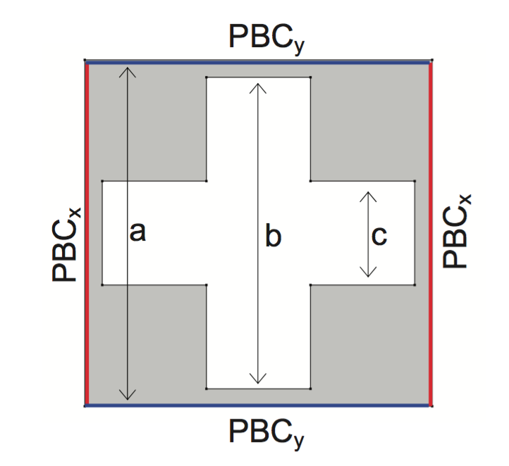
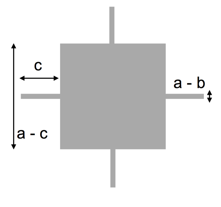
(a)	(b)

Figure 2: (a): Topology and elastic properties of a specific metamaterial exhibiting band-gaps. The grey region is filled by aluminum, the white region is empty. (b): Equivalent periodic building block of the considered phononic structure allowing a more direct identification of the mass-spring mechanism at the microstructural level.

a	b	c	$\rho$	$E$	$\nu$
[$\mathrm{mm}$]	[$\mathrm{mm}$]	[$\mathrm{mm}$]	[$\mathrm{kg/m^{3}}$]	[$\mathrm{GPa}$]	[$-$]
$1$	$0.9$	$0.3$	$2700$	$70$	$0.33$

Table 2: Values of the elastic parameters of the base material (aluminum) and geometric parameters relative to the unit cell shown in Fig. 2.

The unit cell shown in Fig. 2 (a) is clearly equivalent to the one presented in Fig. 2 (b) which can be more directly interpreted as a mass-spring system. This mass-spring representation can be useful when one wants to apply classical homogenization methods to the considered periodic structure. Indeed, following upscaling methods like the ones presented in [2, 6, 7], some informations relative to the micro-mechanisms activated at low frequency (large wavelengths allowing the so-called separation of scale hypothesis) could be disclosed and this would permit a clearer interpretation of some of the parameters of the homogenized relaxed micromorphic model. The problem of establishing such first micro-macro relationships will be the aim of a subsequent work, since we are interested here in the description of the metamaterial at the macroscopic level without restrictions on the frequency (or, equivalently on the wavelength). Indeed, with the methods presented here, we are able to recover the behavior of the metamaterial when excited at wavelengths which go down to the size of the periodic unit cell.

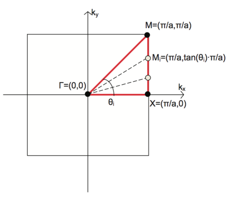
Figure 3: Possible wave paths spanning in the Brillouin zone. We indicate by $\theta_{i}$ the angle that the direction of propagation of the wave $i$ forms with the $x$ direction.

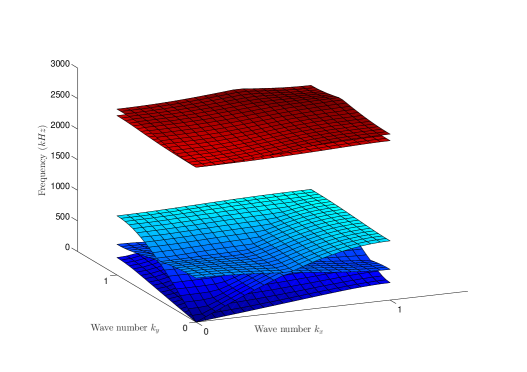
Figure 4: Dispersion surfaces as obtained by the application of Bloch boundary conditions to the unit cell shown in Fig. 2.

A Bloch analysis has been performed (see e.g. [10, 16, 15]) on such metamaterial for waves traveling in the $\Gamma X$, $\Gamma M$ and $XM$ of the usual Brillouin zone, as well as for waves traveling in arbitrary directions within the Brillouin zone (see Fig. 3). As a result of such analysis, the dispersion surfaces for the considered metamaterial have been obtained and are shown in Fig. 4. It can be noticed from Fig. 4 that considering an arbitrary wave-vector of components $(k_{x},k_{y})$ (which means a wave traveling in an arbitrary direction with associated angle $\theta_{i}$), very few changes can be observed on the dispersion curves, especially for those which are bounding the band-gap region. This means that the behavior of the material can be considered not far to be isotropic, even if some low degree of anisotropy of course exists. In this paper, we hence suppose that the considered metamaterial has an isotropic behavior, so that it is reasonable to use the constitutive form (1) of the energy to model it through our enriched continuum model.

To better illustrate our choice of using an isotropic model for the considered metamaterial, we present in Fig. 5 the dispersion curves for wave vectors spanning within the Brillouin zone and having different traveling directions.

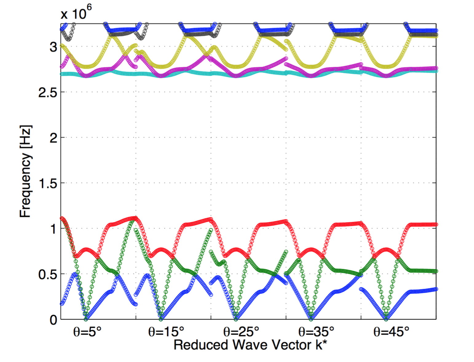
Figure 5: Dispersion curves relative to waves propagating in different directions $\theta_{i}$ within the considered metamaterial. An almost isotropic behavior can be detected, especially concerning the band-gap region.

It can be indeed inferred from Fig. 5 that if some small changes can be observed in the acoustic waves when changing the direction of propagation, almost no change intervenes for the optic curves, in particular for those which bound the band-gap (red and light blue). This observation strengthen our choice of using an isotropic relaxed micromorphic model to characterize the mechanical behavior of the considered metamaterial. Even if the error introduced here using an isotropic model for the considered metamaterial is reasonably small, the problem of studying wave propagation in the anisotropic framework is worth for increasing the number of metamaterials that can be effectively modeled via the relaxed micromorphic model. The case of wave propagation in relaxed micromorphic continua in the anisotropic setting will be treated in further works.

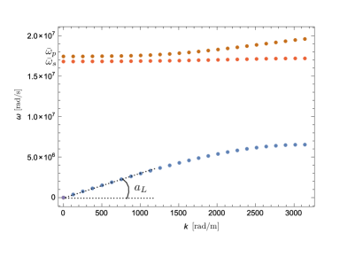
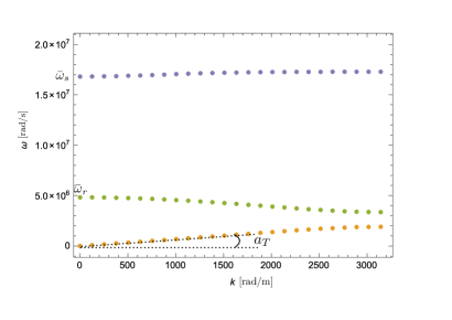
Figure 6: Dispersion curves for the path $\Gamma X$ ($\theta=0$) obtained by means of the code COMSOL^® applying Bloch boundary conditions. Three cut-off frequencies $\bar{\omega}_{s}$, $\bar{\omega}_{p}$ and $\bar{\omega}_{r}$ can be identified.

In Figure 6, we show the dispersion curves for the considered metamaterial relative to a wave traveling in the $\Gamma X$ direction. Such dispersion curves will be those used for the fitting of the parameters of the weighted relaxed micromorphic model. In virtue of the remarks concerning the low anisotropy of the considered metamaterial, the estimate of the parameters on the basis of such curves will be sufficient to start characterizing the metamaterial itself with a reasonable precision. As it was previously said, nevertheless, the fitting on the basis of the dispersion curves alone is not sufficient for a definitive identification of all the elastic coefficients of the considered metamaterial and more accurate fitting procedures based on the transmission coefficient have to be introduced.

3.1 Fitting procedure

The goal that we want to reach finally is that of characterizing the material behavior of the metamaterial shown in Fig.2 by estimating the value of the elastic parameters appearing in the constitutive expression (1) of the strain energy density. To this aim, we present here the fitting procedure that has been used to superimpose the dispersion curves obtained via the relaxed micromorphic model as solutions of equations (33) to the dispersion curves obtained via the Bloch analysis performed by means of the software COMSOL^®.

• The first step has been that of fixing the value of the apparent density $\rho$ of the unit cell. To this purpose, we started calculating the mass $M_{\mathrm{al}}$ of aluminum which is present in each unit cell. With reference to Fig. 2, it is easy to notice that the volume $V_{\mathrm{al}}$ of aluminum present in the unit cell is estimated to be $V_{\mathrm{al}}=4.9\times 10^{-7}\>\mathrm{m}^{3}$. Since the density $\rho_{\mathrm{micro}}$ of the aluminum is known, the mass of aluminum inside the unit cell is easily calculated as $M_{\mathrm{al}}=\rho_{\mathrm{micro}}\,V_{\mathrm{al}}=0.001323\>\mathrm{Kg}.$ Being the volume $V_{\mathrm{macro}}$ of the unit cell known, the apparent density of the unit cell is estimated to be $\rho=M_{\mathrm{al}}/V_{\mathrm{macro}}=1323\>\mathrm{kg/m^{3}}$.

Once the apparent density of the metamaterial has been fixed, the 5 elastic coefficients $\lambda_{e}$, $\mu_{e}$, $\lambda_{\mathrm{micro}}$, $\mu_{\mathrm{micro}}$, $\mu_{c}$ plus the 6 micro-inertia parameters $\eta_{i}$, $\bar{\eta}_{i}$, $i=\left\{1,2,3\right\}$ and characteristic length $L_{c}$ still need to be determined.

• We started setting the characteristic length $L_{c}$ to be vanishing in order to fit the remaining elastic coefficients. Indeed, it was already shown in [25] that $L_{c}$ is related to the non-locality of the metamaterials and its determination is very delicate since, energetically, a non-vanishing $L_{c}$ brings only small corrections to the case with $L_{c}=0$. The value of the other parameters is thus not affected if they are fitted by setting, in a first approximation, $L_{c}=0$. We anticipate the fact that, in the present paper, a reliable value of the non-locality cannot be determined, since the fitting of the parameters on the dispersion curves alone is a tool which is not accurate enough to accomplish this task. In other words, a fitting based on the dispersion curves, if valuable to estimate the elastic parameters, is not sufficient to calibrate the characteristic length which measures non-localities. To this aim, more precise fitting procedures have to be used, such as that of fitting the transmission coefficient obtained via the relaxed micromorphic model to that which is observed experimentally or which is issued by a numerical simulation which accounts for all the elements of the microstructure. In all the remainder of this paper we thus retain the value $L_{c}=0$, simultaneously pointing out that extra investigations of the type presented in [25] are needed to determine the precise value of such parameter.

In order to fit the remaining parameters, we started imposing some conditions that such parameters must necessarily satisfy with the aim of reducing the number of free parameters of the model. In order to obtain such conditions, we remark that:

• With reference to the dispersion curves of the relaxed micromorphic model shown in Fig. 1, the three cut-off frequencies $\omega_{s}$, $\omega_{r}$ and $\omega_{p}$ can be calibrated to coincide with those issued by means of the Bloch analysis shown in Fig. 6. In this latter, we can notice that the lower cut-off frequency $\bar{\omega}_{r}$ is associated to rotational modes and is thus identified with $\omega_{r}$, while the higher cut-off $\bar{\omega}_{p}$ is identified with $\omega_{p}$. Two waves (one longitudinal and one transverse) are seen to have approximately the same cut-off $\bar{\omega}_{s}$ which is thus identified with the characteristic frequency $\text{$\omega$}_{s}$ of the relaxed micromorphic model. Using the definitions (LABEL:eq:characteristic_quantities) we can hence introduce the following equalities that must be satisfied by the parameters of the relaxed micromorphic model (we recall that $\bar{\omega}_{r}$, $\bar{\omega}_{s}$ and $\bar{\omega}_{p}$ are known)

  $$\sqrt{\frac{(3\,\lambda_{e}+2\,\mu_{e})+(3\,\lambda_{\mathrm{micro}}+2\,\mu_{\mathrm{micro}})}{\eta_{3}}}=\bar{\omega}_{p},\qquad\sqrt{\frac{2\,(\mu_{e}+\mu_{\mathrm{micro}})}{\eta_{1}}}=\bar{\omega}_{s},\qquad\sqrt{\frac{2\,\mu_{c}}{\eta_{2}}}=\bar{\omega}_{r}.$$ (36)

• We want also to impose that the slope of the acoustic curves of the micromorphic model is the same as that obtained via the Bloch analysis. To do so, with reference to Eqs. (LABEL:eq:SlopesLT) we impose that

  $$\sqrt{\frac{3\,\lambda_{e}\,\lambda_{\mathrm{micro}}\,(\mu_{e}+\mu_{\mathrm{micro}})+2\mu_{e}\,\mu_{\mathrm{micro}}\left[3(\lambda_{e}+\lambda_{\mathrm{micro}})+2(\mu_{e}+\mu_{\mathrm{micro}})\right]+2\lambda_{\mathrm{micro}}\,\mu_{e}^{2}+2\lambda_{e}\,\mu_{\mathrm{micro}}^{2}}{\rho\,(\mu_{e}+\mu_{\mathrm{micro}})\left(3(\lambda_{e}+\lambda_{\mathrm{micro}})+2(\mu_{e}+\mu_{\mathrm{micro}})\right)}}=a_{L},$$

  $$\sqrt{\frac{\mu_{e}\,\mu_{\mathrm{micro}}}{\rho\,(\mu_{e}+\mu_{\mathrm{micro}})}}=a_{T},$$

  where $a_{L}$ and $a_{T}$ are the numerical values of the slopes of the acoustic longitudinal and transverse branches, respectively, as obtained via the Bloch analysis.

By solving equations (36), (LABEL:eq:Imposizione_2) with respect to a suitable subset of the unknown parameters, we find the following solution

$$\mu_{c}=\frac{\bar{\omega}_{r}^{2}}{2}\eta_{2},\qquad\mu_{e}=\frac{\rho\,a_{T}^{2}\,\mu_{\mathrm{micro}}}{\mu_{\mathrm{micro}}-\rho a_{T}^{2}},\qquad\lambda_{e}=-\lambda_{\mathrm{micro}}+\frac{2}{3}\frac{\mu_{\mathrm{micro}}^{2}}{-\mu_{\mathrm{micro}}+\rho\,a_{T}^{2}}+\frac{\left(3\,\lambda_{\mathrm{micro}}+2\,\mu_{\mathrm{micro}}\right)^{2}}{3\,\left(3\,\lambda_{\mathrm{micro}}+2\,\mu_{\mathrm{micro}}-3\rho\,a_{L}^{2}+4\rho a_{T}^{2}\right)},$$

$$\eta_{1}=\frac{2\mu_{\mathrm{micro}}^{2}}{\left(\mu_{\mathrm{micro}}-\rho a_{T}^{2}\right)\bar{\omega}_{s}^{2}},\qquad\eta_{3}=\frac{\left(3\lambda_{\mathrm{micro}}+2\mu_{\mathrm{micro}}\right)^{2}}{\left(3\lambda_{\mathrm{micro}}+2\mu_{\mathrm{micro}}-3\rho\,a_{L}^{2}+4\rho\,a_{T}^{2}\right)\bar{\omega}_{p}^{2}}.$$

The parameters of the model which remain still free are thus $\lambda_{\mathrm{micro}}$, $\mu_{\mathrm{micro}}$, $\eta_{2}$, $\bar{\eta}_{1}$, $\bar{\eta}_{2}$ and $\bar{\eta}_{3}$. The last two equations can also be inverted in order to find $\lambda_{\mathrm{micro}}$ and $\mu_{\mathrm{micro}}$ as functions of $\eta_{1}$ and $\eta_{3}$, which is a more desirable situation to perform the fitting procedure. In this way, the free parameters to be varied for the fitting procedures would be only the free and gradient micro inertias $\eta_{1}$, $\eta_{2}$, $\eta_{3}$, $\bar{\eta}_{1}$, $\bar{\eta}_{2}$ and $\bar{\eta}_{3}$. Indeed, regarding the last two equations (LABEL:eq:partial_Solution) in such a way to solve them in terms of $\mu_{\mathrm{micro}}$ and $\lambda{}_{\mathrm{micro}}\,$, we get the following solutions

$$\mu_{\mathrm{micro}} =\frac{1}{4}\left(\eta_{1}\bar{\omega}_{s}^{2}\pm\sqrt{\eta_{1}\bar{\omega}_{s}^{2}\,(-8\,\rho\,a_{T}^{2}+\eta_{1}\bar{\omega}_{s}^{2})}\right),$$

$$\lambda_{\mathrm{micro}} =\frac{1}{6}\left(-4\mu_{\mathrm{micro}}+\eta_{3}\bar{\omega}_{p}^{2}\pm\sqrt{\eta_{3}\bar{\omega}_{p}^{2}\,(-12\,\rho\,a_{L}^{2}+16\,\rho\,a_{T}^{2}+\eta_{3}\bar{\omega}_{p}^{2})}\right).$$

This means that, for any arbitrary value of $\eta_{1}$ and $\eta_{3}$, there are two possible values of $\mu_{\mathrm{micro}}$ and hence four possible values of $\lambda{}_{\mathrm{micro}}\,$. In other words, If we think to vary the values of $\eta_{1}$ and $\eta_{3}$, four different possible solutions arise and one among them must be chosen on the basis of experimental observations. Since, as a physical requirement, $\mu_{\mathrm{micro}}$ and $\lambda{}_{\mathrm{micro}}\,$ must be real, then some restrictions on $\eta_{1}$ and $\eta_{3}$ have to be imposed in order to avoid complex solutions for such elastic coefficients. It can be remarked that, on the basis of Eqs. (LABEL:eq:conditions), the following conditions must be imposed on the micro-inertias $\eta_{1}$ and $\eta_{3}$ in order to guarantee that $\mu_{\mathrm{micro}}$ and $\lambda{}_{\mathrm{micro}}\,$ take only real values

$$\eta_{1}>\frac{8\,\rho\,a_{T}^{2}}{\bar{\omega}_{s}^{2}},\qquad\eta_{3}>\frac{4\,\rho\left(3\,a_{L}^{2}-4\,a_{T}^{2}\right)}{\bar{\omega}_{p}^{2}}\>.$$ (40)

Such conditions suggest the minimal numerical values for $\eta_{1}$ and $\eta_{2}$ which must be used to start the fitting procedure. The value of the two micro-inertias $\eta_{1}$ and $\eta_{2}$ will be in fact slowly increased starting from their minimal value in order to fit the dispersion curves of the relaxed micromorphic model on those obtained via the Bloch analysis.

In order to fit at best the remaining free parameters $\eta_{1}$, $\eta_{2}$, $\eta_{3}$, $\bar{\eta}_{1}$, $\bar{\eta}_{2}$, $\bar{\eta}_{3}$, we have performed a systematic numerical check to unveil eventual peculiar effects of each parameter on the dispersion curves. The fitting procedure has been performed as follows

• The characteristic effect of each parameter on the dispersion curves is searched by slightly increasing each of them starting from the initial values

  $$\eta_{1}=\frac{8\,\rho\,,a_{T}^{2}}{\bar{\omega}_{s}^{2}},\quad\eta_{2}=0,\quad\eta_{3}=\frac{4\,\rho\left(3\,a_{L}^{2}-4\,a_{T}^{2}\right)}{\bar{\omega}_{p}^{2}},\quad\bar{\eta}_{1}=0,\quad\bar{\eta}_{2}=0,\quad\bar{\eta}_{3}=0.$$

• It is found that $\eta_{1}$ has a visible effect on the optic curves $LO_{1}$ and $TO_{1}$ as well as a smaller effect on the acoustic curves $LA$ and $TA$. The parameter $\eta_{1}$ is then carefully increased in order to reach the best possible agreement with the acoustic curves as well as with the curves $LO_{1}$ and $TO_{1}$. A rather good agreement is found (for one of the four possible solutions) for all the aforementioned curves for a first tentative value of $\eta_{1}$, except for the curve $LO_{1}$ that drastically diverge from that issued by the discrete simulation, above all for high wavenumbers.

• The parameter $\bar{\eta}_{3}$ is seen to have a flattening effect on the longitudinal curves. Increasing this parameter allows a better fitting of the curve $LO_{1}$ which was still remaining to be better adjusted from the previous step.

• The gradient micro-inertia parameter $\bar{\eta}_{1}$ has the effect of flattening simultaneously the longitudinal and transverse waves. This effect is not desirable since the transverse curves are already well-fitted at this stage. We then set $\bar{\eta}_{1}$ to be identically vanishing.

• The parameter $\eta_{2}$ is seen to have an effect on the curves $TO_{2}$ and $TA$. In particular, for some values of $\eta_{2}$, the curve $TO_{2}$ is seen to be almost flat. This is the best agreement that we can find with the curve issued via the Bloch wave analysis, which is instead slightly decreasing. Up to now, the introduced formulation of the relaxed micromorphic model does not allow to obtain dispersion branches which decrease when increasing the wavenumber, thus the best approximation is obtained with an almost horizontal line. We will discuss the possibility of obtaining such decreasing curves in the framework of the relaxed micromorphic model in subsequent works. In order to get the best average fitting of the curve $TO_{2}$, we slightly relax the third of conditions (36) in order to impose a cut-off which takes a lower value than the exact value $\bar{\omega}_{r}$. We also remark that, indeed, the desired horizontal curve $TO_{2}$ can be obtained for an infinite set of values of $\eta_{2}$. As a consequence, there exist an infinity of calculated values of the Cosserat couple modulus $\mu_{c}$ (via the third of conditions (36)) which correspond to such set of values of $\eta_{2}$. This indeterminacy on the value of $\eta_{2}$ (and thus of $\mu_{c}$) is strongly related to the fact that we cannot generate decreasing curves within the relaxed micromorphic model. This issue will be solved in a subsequent work. At the present stage, we chose to fix the value of the micro-rotation inertia $\eta_{2}$ to be the same of the micro-distortion inertia $\eta_{1}$ (which actually produces the desired horizontal $TO_{2}$ curve) and we thus compute the corresponding value of $\mu_{c}$. Except for this indeterminacy on the parameters $\eta_{2}$ and $\mu_{c}$, all the remaining parameters of the model are uniquely calibrated.

• The parameter $\eta_{3}$ is seen to have a non-negligible effect on the optic curve $LO_{2}$ and on the longitudinal acoustic curve $LA$ and is hence adjusted in order to obtain the best possible fitting. On the other hand, the parameter $\bar{\eta}_{2}$ is seen to have the opposite effect on the curve $LO_{2}$ as well as a slight effect on the curve $TA$. The parameters $\eta_{3}$ and $\bar{\eta}_{2}$ are then carefully calibrated in order to get the best possible agreement of the curve $LO_{2}$ without macroscopically perturbing the other curves affected by such parameters.

• The found set of values for $\eta_{1}$, $\eta_{2}$, $\eta_{3}$, $\bar{\eta}_{1}$, $\bar{\eta}_{2}$, $\bar{\eta}_{3}$, is then slightly arranged for a last refined fitting. The obtained numerical values are shown in Table (3). The remaining parameters of the model can also be determined by means of the relations (LABEL:eq:partial_Solution) and are shown in Table (4).

$\eta_{1}$	$\eta_{2}$	$\eta_{3}$	$\bar{\eta}_{1}$	$\bar{\eta}_{2}$	$\bar{\eta}_{3}$
$\left[\mathrm{kg/m}\right]$	$\left[\mathrm{kg/m}\right]$	$\left[\mathrm{kg/m}\right]$	$\left[\mathrm{kg/m}\right]$	$\left[\mathrm{kg/m}\right]$	$\left[\mathrm{kg/m}\right]$
$3.25\times 10^{-5}$	$3.25\times 10^{-5}$	$4\times 10^{-4}$	$0$	$0.3\times 10^{-4}$	$1.8\times 10^{-4}$

Table 3: Values of the micro-inertia parameters of the weighted relaxed micromorphic model as fitted on the metamaterial shown in Figure 2.

$\rho$	$\mu_{c}$	$\lambda_{\mathrm{micro}}$	$\mu_{\mathrm{micro}}$	$\lambda_{e}$	$\mu_{e}$	$L_{c}$
$\left[\mathrm{kg/m^{3}}\right]$	$\left[\mathrm{GPa}\right]$	$\left[\mathrm{GPa}\right]$	$\left[\mathrm{GPa}\right]$	$\left[\mathrm{GPa}\right]$	$\left[\mathrm{GPa}\right]$	$\left[\mathrm{m}\right]$
$1323$	$0.272$	$19.8$	$0.737$	$17.7$	$3.857$	$0$

Table 4: Values of the parameters of the weighted relaxed micromorphic model for the metamaterial shown in Figure 2.

The final fitting of the parameters of the relaxed micromorphic model on the curves issued by the Bloch wave analysis is shown in Figure (7). An almost perfect fitting is obtained for all the curves, with the exception of some small deviations of the $TO_{2}$ curve which cannot at the present stage be arranged to be a decreasing curve. This last detail will be fixed in subsequent works.

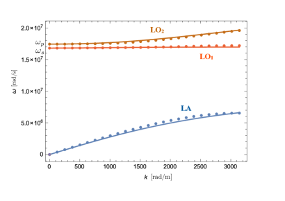
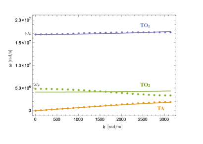
Figure 7: Fitting of the curves obtained via the weighted relaxed micromorphic model (continuous lines) on the dispersion curves issued via the Bloch wave analysis (dotted curves), for wavenumbers up to the size of the unitary cell. Left: longitudinal waves; Right: transverse waves.

According to the fitted values of the parameters and considering formulas (35), it is also possible to derive, a posteriori, the value of the averaged macroscopic parameters of the considered metamaterial, which are shown in Table 5.

$\lambda_{\mathrm{macro}}$	$\mu_{\mathrm{macro}}$
$\left[\mathrm{GPa}\right]$	$\left[\mathrm{GPa}\right]$
$0.62$	$4.66$

$E_{\mathrm{macro}}$	$\nu_{\mathrm{macro}}$
$\left[\mathrm{GPa}\right]$	$\left[-\right]$
$1.78$	$0.44$

Table 5: Values of the macroscopic parameters of the considered metamaterial computed starting from the values shown in Tables 3 and 4 and using the homogenization formulas (35) (left) and corresponding values of the Young modulus and Poisson ratio (right).

It is possible to notice, comparing the values of the parameters of the metamaterial given in Table 5 with those of the original material (aluminum) shown in Table 2, that the presence of the cross cavity renders the resulting metamaterial softer than the original one. Also the Poisson’s effect results to be enhanced in the metamaterial compared to the original material.

3.2 Analysis of the vibrational modes

In this subsection we analyze the vibrational modes of the considered metamaterial as function of the frequency and of the wavelength, both theoretically via the relaxed micromorphic model and by using the Bloch wave analysis.

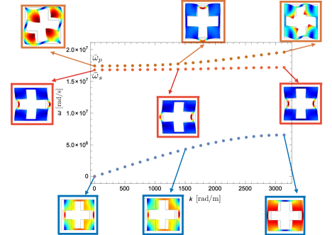
Figure 8: Vibrational modes for longitudinal waves as function of the wavenumber obtained via Bloch wave analysis.

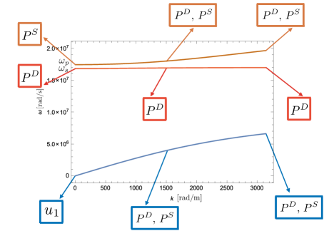
Figure 9: Qualitative distribution of the theoretical vibration modes for longitudinal waves obtained via the relaxed micromorphic model as function of the wavenumber.

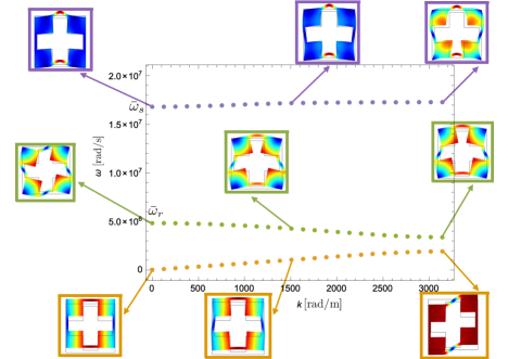
Figure 10: Vibrational modes for transverse waves as function of the wavenumber obtained via Bloch wave analysis.

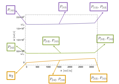
Figure 11: Qualitative distribution of the theoretical vibration modes for transverse waves obtained via the relaxed micromorphic model as function of the wavenumber.

Indeed, it is well known that the vibrational modes of the unit cell of periodic metamaterials vary when varying the wavelength of the traveling wave. This can be recognized in Figure 8 where the main vibrational modes of the unit cell are depicted as function of the wavenumber up to the size of the unit cell. It can be recognized that for the longitudinal and transverse acoustic waves, the main vibrational modes are given by horizontal and transverse macroscopic displacements of the unit cell when considering very large wavelength (small $k$). When increasing the wavenumber (reducing the wavelength) we can observe from Figures 8 and 10 that for $k\sim 1500\,\mathrm{rad/m}^{-1}$ the microstructure-related acoustic vibrational modes start to take a predominant role. This means that the unit cell is not only displaced of a given amount, but also starts deforming. Volume variations coupled to micro-distortion of the unit cell can be observed for the longitudinal modes, while micro-rotations coupled to in-plane shear are found for the transverse modes. Analogous patterns can be obtained via the relaxed micromorphic model when normalizing the eigenvectors corresponding to the eigenvalues shown in Figure 7. In particular, the agreement of the vibrational modes found via the relaxed micromorphic model with those issued via the Bloch analysis can be deciphered when recalling that

• $P^{S}$ is the spherical part of the micro-distortion tensor related to volume variations,

• $P^{D}$ is related to the deviatoric part of the micro-distortion tensor which is known to be associated to the actual distortion of the unit cell

• $P_{(12)}$ is the $(1,2)$ component of the symmetric part of the micro-distortion tensor which can be directly related to in-plane shear of the unit cell,

• $P_{[12]}$ is the $(1,2)$ component of the skew-symmetric part of the micro-distortion tensor which is known to be related to in-plane rotations of the microstruture embedded in the unit cell.

4 Conclusions

In this paper we study the macroscopic behavior of real band-gap metamaterials by using the linearized, isotropic relaxed micromorphic model with weighted free and gradient micro-inertia. For a specific microstructure, we make a direct comparison between the dispersion curves issued via the classical Bloch wave analysis and those obtained by means of our weighted relaxed micromorphic model. Such comparison allows us to uniquely identify almost all the parameters of the model with the exception of the characteristic length $L_{c}$ and of the Cosserat couple modulus $\mu_{c}$. In particular, the characteristic length $L_{c}$ is a very sensitive parameter measuring the non-locality of the considered metamaterial, the determination of which requires a much more refined fitting procedure than that which is possible on the basis of the dispersion curves alone. A more refined fitting based e.g. on the energy which is transmitted through the considered metamaterial for different frequencies is needed, as done e.g. in [25]. The determination of the characteristic length of the metamaterial targeted in this paper will be then analyzed in subsequent works, given that the measure of all the remaining parameters is not affected by the determination of $L_{c}$.

On the other hand, the Cosserat couple modulus $\mu_{c}$ is found to be directly proportional to the micro-inertia parameter $\eta_{2}$ (related to the skew-symmetric part of the tensor $P_{,t}$). Nevertheless, the performed fitting does not allow to uniquely conclude about the value of $\mu_{c}$. Choosing the rotational micro-inertia $\eta_{2}$ to be equal to the distortion micro-inertia $\eta_{1}$, we are able to deduce the corresponding value of $\mu_{c}$. To allow a more precise fitting of $\mu_{c}$, the relaxed micromorphic model needs to be further generalized in order to grant the possibility of dispersion curves which are decreasing for increasing wavenumber $k$. Such a generalization of the relaxed micromorphic model will be the focus of subsequent works.

The results presented in this paper represent a topical breakthrough allowing a simple implementation of the relaxed micromorphic model in finite element codes in view of meta-structural design.

5 Acknowledgments

Angela Madeo thanks INSA-Lyon for the funding of the BQR 2016 "Caractérisation mécanique inverse des métamatériaux: modélisation, identification expérimentale des paramètres et évolutions possibles", as well as the CNRS-INSIS for the funding of the PEPS project.

References

- [1] Mario N. Armenise, Carlo E. Campanella, Caterina Ciminelli, Francesco Dell’Olio, and Vittorio M. N. Passaro. Phononic and photonic band gap structures: Modelling and applications. Physics Procedia, 3(1):357–364, 2010.
- [2] Jean Louis Auriault and Claude Boutin. Long wavelength inner-resonance cut-off frequencies in elastic composite materials. International Journal of Solids and Structures, 49(23-24):3269–3281, 2012.
- [3] Gabriele Barbagallo, Marco Valerio d’Agostino, Rafael Abreu, Ionel-Dumitrel Ghiba, Angela Madeo, and Patrizio Neff. Transparent anisotropy for the relaxed micromorphic model: macroscopic consistency conditions and long wave length asymptotics. Preprint ArXiv, 1601.03667, 2016.
- [4] Davide Bigoni, Sébastien Guenneau, Alexander B. Movchan, and Morvan Brun. Elastic metamaterials with inertial locally resonant structures: Application to lensing and localization. Phys. Rev. B, 87(17):174303, 2013.
- [5] Alvaro Blanco, Emmanuel Chomski, Serguei Grabtchak, Marta Ibisate, Sajeev John, Stephen W. Leonard, Cefe Lopez, Francisco Meseguer, Hernan Miguez, Jessica P. Mondia, Geoffrey A. Ozin, Ovidiu Toader, and van Driel Henry M. Large-scale synthesis of a silicon photonic crystal with a complete three-dimensional bandgap near 1.5 micrometres. Nature, 405(6785):437–40, 2000.
- [6] Claude Boutin and Stéphane Hans. Homogenisation of periodic discrete medium: Application to dynamics of framed structures. Computers and Geotechnics, 30(4):303–320, 2003.
- [7] Claude Boutin, Stéphane Hans, and Céline Chesnais. Generalized Beams and Continua. Dynamics of Reticulated Structures, pages 131–141. Springer New York, New York, NY, 2010.
- [8] Claude Boutin and Jean Soubestre. Generalized inner bending continua for linear fiber reinforced materials. International Journal of Solids and Structures, 48(3-4):517–534, 2011.
- [9] Morvan Brun, Sébastien Guenneau, Alexander B. Movchan, and Davide Bigoni. Dynamics of structural interfaces: Filtering and focussing effects for elastic waves. Journal of the Mechanics and Physics of Solids, 58(9):1212–1224, 2010.
- [10] Manuel Collet, Morvan Ouisse, Massimo Ruzzene, and Mohamed Ichchou. Floquet-Bloch decomposition for the computation of dispersion of two-dimensional periodic, damped mechanical systems. International Journal of Solids and Structures, 48(20):2837–2848, 2011.
- [11] Andrea Colombi, Daniel J. Colquitt, Philippe Roux, Sébastien Guenneau, and Richard V. Craster. A seismic metamaterial: The resonant metawedge. Scientific Reports, 6(Umr 7249):27717, jun 2016.
- [12] Daniel J. Colquitt, Morvan Brun, Massimiliano Gei, Alexander B. Movchan, Natasha V. Movchan, and Ian Samuel Jones. Transformation elastodynamics and cloaking for flexural waves. Journal of the Mechanics and Physics of Solids, 72:131–143, 2014.
- [13] Richard V. Craster and Sébastien Guenneau. Acoustic Metamaterials: Negative Refraction, Imaging, Lensing and Cloaking. page 332. 2013.
- [14] Marco Valerio d’Agostino, Gabriele Barbagallo, Ionel-Dumitrel Ghiba, Angela Madeo, and Patrizio Neff. A panorama of dispersion curves for the isotropic weighted relaxed micromorphic model. Preprint ArXiv, 2016.
- [15] Yu Fan, Manuel Collet, Mohamed Ichchou, Lin Li, Olivier Bareille, and Zoran Dimitrijevic. A wave-based design of semi-active piezoelectric composites for broadband vibration control. Smart Materials and Structures, 25(5):055032, 2016.
- [16] Yu Fan, Manuel Collet, Mohamed Ichchou, Lin Li, Olivier Bareille, and Zoran Dimitrijevic. Energy flow prediction in built-up structures through a hybrid finite element/wave and finite element approach. Mechanical Systems and Signal Processing, 66-67:137–158, 2016.
- [17] Marian Florescu, Salvatore Torquato, and Paul J. Steinhardt. Complete band gaps in two-dimensional photonic quasicrystals. Physical Review B - Condensed Matter and Materials Physics, 80(15):1–7, 2009.
- [18] Marian Florescu, Salvatore Torquato, and Paul J. Steinhardt. Designer disordered materials with large, complete photonic band gaps. Proceedings of the National Academy of Sciences of the United States of America, 106(49):20658–20663, 2009.
- [19] Ionel-Dumitrel Ghiba, Patrizio Neff, Angela Madeo, Luca Placidi, and Giuseppe Rosi. The relaxed linear micromorphic continuum: existence, uniqueness and continuous dependence in dynamics. Mathematics and Mechanics of Solids, 20(10):1171–1197, 2014.
- [20] Jakub Haberko and Frank Scheffold. Fabrication of mesoscale polymeric templates for three-dimensional disordered photonic materials. Optics express, 21(1):1057–65, 2013.
- [21] Jiankun Huang and Zhifei Shi. Attenuation zones of periodic pile barriers and its application in vibration reduction for plane waves. Journal of Sound and Vibration, 332(19), 2013.
- [22] Noe Jiménez, Weichun Huang, Vicent Romero-García, Vicent Pagneux, and Jean-Philippe Groby. Ultra-thin metamaterial for perfect and quasi-omnidirectional sound absorption. Applied Physics Letters, 109(12):121902, 2016.
- [23] Shawn-Yu Lin and James G. Fleming. A three-dimensional optical photonic crystal. Journal of Lightwave Technology, 17(11):1944–1947, 1999.
- [24] Zhengyou Liu, Xixiang Zhang, Yiwei Mao, Y. Y. Zhu, Zhiyu Yang, C. T. Chan, and Ping Sheng. Locally resonant sonic materials. Science, 289(5485):1734–1736, 2000.
- [25] Angela Madeo, Gabriele Barbagallo, Marco Valerio d’Agostino, Luca Placidi, and Patrizio Neff. First evidence of non-locality in real band-gap metamaterials: determining parameters in the relaxed micromorphic model. Proceedings of the Royal Society A: Mathematical, Physical and Engineering Sciences, 472(2190):20160169, 2016.
- [26] Angela Madeo, Patrizio Neff, Elias C. Aifantis, Gabriele Barbagallo, and Marco Valerio d’Agostino. On the role of micro-inertia in enriched continuum mechanics. Preprint ArXiv, 1607.07385, 2016.
- [27] Angela Madeo, Patrizio Neff, Marco Valerio d’Agostino, and Gabriele Barbagallo. Complete band gaps including non-local effects occur only in the relaxed micromorphic model. Comptes Rendus Mécanique, 2016.
- [28] Angela Madeo, Patrizio Neff, Ionel-Dumitrel Ghiba, Luca Placidi, and Giuseppe Rosi. Band gaps in the relaxed linear micromorphic continuum. Zeitschrift für Angewandte Mathematik und Mechanik, 95(9):880–887, 2014.
- [29] Angela Madeo, Patrizio Neff, Ionel-Dumitrel Ghiba, Luca Placidi, and Giuseppe Rosi. Wave propagation in relaxed micromorphic continua: modeling metamaterials with frequency band-gaps. Continuum Mechanics and Thermodynamics, 27(4-5):551–570, 2015.
- [30] Angela Madeo, Patrizio Neff, Ionel-Dumitrel Ghiba, and Giuseppe Rosi. Reflection and transmission of elastic waves in non-local band-gap metamaterials: a comprehensive study via the relaxed micromorphic model. Journal of the Mechanics and Physics of Solids, 95:441–479, 2016.
- [31] Martin Maldovan. Sound and heat revolutions in phononics. Nature, 503(7475):209–217, 2013.
- [32] Weining Man, Marian Florescu, Kazue Matsuyama, Polin Yadak, Geev Nahal, Seyed Hashemizad, Eric Williamson, Paul Steinhardt, Salvatore Torquato, and Paul Chaikin. Photonic band gap in isotropic hyperuniform disordered solids with low dielectric contrast. Optics Express, 21(17):19972–81, 2013.
- [33] Rosa Martínez-Sala, J. Sancho, Juan V. Sánchez, Vicente Gómez, J. Llinares, and Francisco Meseguer. Sound attenuation by sculpture. Nature, 378(6554):241–241, 1995.
- [34] Marco Miniaci, Anastasiia Krushynska, Federico Bosia, and Nicola M Pugno. Large scale mechanical metamaterials as seismic shields. New Journal of Physics, 18(8):83041, 2016.
- [35] Diego Misseroni, Daniel J. Colquitt, Alexander B. Movchan, Natasha V. Movchan, and Ian Samuel Jones. Cymatics for the cloaking of flexural vibrations in a structured plate. Scientific Reports, 6(23929), 2016.
- [36] Federica Morandi, Marco Miniaci, Alessandro Marzani, Luca Barbaresi, and Massimo Garai. Standardised acoustic characterisation of sonic crystals noise barriers: Sound insulation and reflection properties. Applied Acoustics, 114:294–306, 2016.
- [37] Bruno Morvan, Alain Tinel, Anne Christine Hladky-Hennion, Jérôme Vasseur, and Bertrand Dubus. Experimental demonstration of the negative refraction of a transverse elastic wave in a two-dimensional solid phononic crystal. Applied Physics Letters, 96(10):2008–2011, 2010.
- [38] Patrizio Neff. The Cosserat couple modulus for continuous solids is zero viz the linearized Cauchy-stress tensor is symmetric. Zeitschrift für Angewandte Mathematik und Mechanik, 86(11):892–912, 2006.
- [39] Patrizio Neff, Ionel-Dumitrel Ghiba, Markus Lazar, and Angela Madeo. The relaxed linear micromorphic continuum: well-posedness of the static problem and relations to the gauge theory of dislocations. The Quarterly Journal of Mechanics and Applied Mathematics, 68(1):53–84, 2015.
- [40] Patrizio Neff, Ionel-Dumitrel Ghiba, Angela Madeo, Luca Placidi, and Giuseppe Rosi. A unifying perspective: the relaxed linear micromorphic continuum. Continuum Mechanics and Thermodynamics, 26(5):639–681, 2014.
- [41] John B. Pendry. Negative refraction makes a perfect lens. Phys. Rev. Lett., 85(18):3966–3969, 2000.
- [42] John B. Pendry, David Schurig, and David R. Smith. Controlling electromagnetic fields. Science, 312(5781):1780–1782, 2006.
- [43] Kim Pham, Varvara G. Kouznetsova, and Marc G. D. Geers. Transient computational homogenization for heterogeneous materials under dynamic excitation. Journal of the Mechanics and Physics of Solids, 61(11):2125–2146, 2013.
- [44] Alessandro Spadoni, Massimo Ruzzene, Stefano Gonella, and Fabrizio Scarpa. Phononic properties of hexagonal chiral lattices. Wave Motion, 46(7):435–450, 2009.
- [45] Ashwin Sridhar, Varvara G. Kouznetsova, and Marc G. D. Geers. Homogenization of locally resonant acoustic metamaterials towards an emergent enriched continuum. Computational Mechanics, 57(3):423–435, 2016.
- [46] Yan-Feng Wang and Yue-Sheng Wang. Multiple wide complete bandgaps of two-dimensional phononic crystal slabs with cross-like holes. Journal of Sound and Vibration, 332(8):2019–2037, 2013.
- [47] Eli Yablonovitch. Photonic band-gap structures. J. Opt. Soc. Am. B, 10(2):283–295, 1993.
- [48] Noritsugu Yamamoto and Susumu Noda. Fabrication and optical properties of one period of a three-dimensional photonic crystal operating in the 5 – 10 m wavelength region. Japanese Journal of Applied Physics, 38(2):1282–1285, 1999.
- [49] Kaijun Yi, Manuel Collet, Mohamed Ichchou, and Lin Li. Flexural waves focusing through shunted piezoelectric patches. Smart Materials and Structures, 25(7):075007, 2016.