Electronic structure of graphene: (nearly) free electrons bands vs. tight-binding bands

Abstract

In our previous paper (Phys. Rev. B 89, 165430 (2014)) we have found that in graphene, in distinction to the four occupied bands, which can be described by the simple tight-binding model (TBM) with four atomic orbitals per atom, the two lowest lying at the $\Gamma$-point unoccupied bands (one of them of a $\sigma$ type and the other of a $\pi$ type) can not be described by such model. In the present work we suggest a minimalistic model for these two bands, based on (nearly) free electrons model (FEM), which correctly describes the symmetry of these bands, their dispersion law and their localization with respect to the graphene plane.

I Introduction

In the course of the study of graphite and a graphite monolayer, called graphene, understanding of the symmetries of the electron dispersion law in graphene was of crucial importance. Actually, the symmetry classification of the energy bands in graphene was presented nearly 60 years ago by Lomer in his seminal paper 1 . Later the subject was analyzed by Slonczewski and Weiss 2 , Dresselhaus and Dresselhaus 3 , Bassani and Parravicini 4 , Malard et al 5 , Manes 6 and others. Note that the first attempt to apply the TBM to the calculation of the electrons dispersion law in graphene (graphite) was done already in 1935 by F. Hund and B. Mrowka hund .

In our previous publication kogan we compared the classification of the electron bands in graphene, obtained by group theory algebra in the framework of a tight-binding model (TBM), with that calculated in a density-functional-theory (DFT) local-density approximation framework. Identification in the DFT band structure of all eight energy bands (four valence and four conduction bands) corresponding to the TBM-derived energy bands was performed and the corresponding analysis was presented. The four occupied (three $\sigma$ -like and one $\pi$ -like) and three unoccupied (two $\sigma$ -like and one $\pi$ -like) bands given by the DFT closely correspond to those predicted by the TBM, both by their symmetry and their dispersion law. However, the two lowest lying at the $\Gamma$-point unoccupied bands (one of them of a $\sigma$ -like type and the other of a $\pi$-like one), were found to be not of the TBM type in accord with the earlier publications pobaprl83 ; pobaprl84 ; wegrprl08 . Moreover, recently it was shown that indeed these two states resemble the lowest-energy members of the image-potential states series predicted to exist in vicinity of the graphene monolayer when the potential shape on the vacuum side is modified to a correct asymptotic $\sim-1/4z$ behavior sizhprb09 . Indeed such unoccupied image-potential states at the solid surfaces ecpejpc78 were a subject of extensive theoretical and experimental investigation during several decades dast92 ; farecp00 ; ecbessr04 . Recently image-potential states were observed on graphene absorbed on different substrates bobaprl10 ; zhhujpcm10 ; nifaprb12 ; arguprl12 ; nopoprb13 ; crruprl13 ; nifajpcm14 , whereas the two lowest-energy members of an image series of a pure graphene were detected for graphene placed of a SiC surface bosinjp10 ; taimprb14 ; shjoapl14 . Moreover a transformation of such states in carbon nanotubes and fullerenes fezhs08 ; zhfeacsn09 or an evolution of the lowest-energy symmetric state into a widely discussed interlayer band fahiprl83 ; stblprb00 ; cslinp05 in graphite upon increasing of number of the graphene layers was studied bosinjp10 ; taimprb14 ; codoss16 .

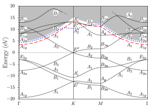
Figure 1: (color online) Graphene band structure. The dotted line shows the Fermi energy. The grey area corresponds to the vacuum continuum states. The non-TBM bands of our interest are plotted with long-dashed (red) and short-dashed (blue) lines. The upper bands merge into scattering resonances of graphene Nazarov-13 ; Wicki-16 , which is schematically shown with dashed (black) endings of lines.

In Fig. 1 we reproduce the results of the band structure calculations with symmetry labelling of the occupied and the lowest lying unoccupied bands. The TBM bands are plotted in solid lines, $\sigma$ non-TBM band - in long dashed, $\pi$ non-TBM band - in dotted line. To understand the symmetry classification of the bands one should remember that the group of wave vector ${\bf k}$ at the $\Gamma$ point is $D_{6h}$; at the $K$ point – $D_{3h}$; at the point $M$ – $D_{2h}$. The group of wave vector ${\bf k}$ at each of the lines constituting triangle $\Gamma-K-M$ is $C_{2v}$ thomsen ; dresselhaus . Representations of the groups can be found in the book by Landau and Lifshitz landau . Honeycomb lattice and its Brillouine zone with the symmetry points are presented on Fig. 2.

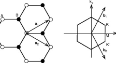
Figure 2: Honeycomb lattice and its Brillouin zone.

One of rotations $U_{2}$ for the $D_{6h}$ group is about the direction $\Gamma-K$. Rotation $C_{2}^{z}$ for the $D_{2h}$ group is about the normal to graphene plane, rotation $C_{2}^{x}$ - about the $\Gamma-M$ line. Reflection $\sigma_{v}$ for the $C_{2v}$ groups is relative to the plane of graphene. The mathematical details of the symmetry analysis in TBM are presented in Section III.

II Free electrons model bands

Let us start this Section from explaining what do we mean by saying that a given electron band is not a tight-binding one. In our previous publication kogan we have pointed that the symmetry of the two low lying unoccupied bands contradicts to the predictions of the tight-binding model (with the four atomic orbitals considered). We have also shown that their localization with respect to graphene plane is drastically different from that of occupied bands and also of $\pi^{*}$ band. In the present Section we make another step in this direction. We point that both the symmetry and the dispersion law of these two bands can be obtained in the framework of the model opposite to the tight-binding model – the (nearly) free electrons model.

The difference between the TBM and non-TBM states is evident from the Figures in our previous publication kogan presenting electron density. The former are localized in the vicinity of graphene plane within a distance of the order of graphene lattice constant $a$. The latter are localized within a distance $\mu a$, where $\mu\gg 1$. It means that while calculating the dispersion law with its typical energy scale $\hbar^{2}/ma^{2}\sim 1$ eV, for the non-TBM bands in zero order approximation with respect to parameter $1/\mu$ we can ignore the $z$ dependence of the wave functions. In addition, when looking on Fig. 1 one notices that the dispersion of the two non-TBM bands follow very closely the continuum bottom lines, which present the dispersion law of the free electrons, staying below them.

Hence we can formulate a minimalistic model for the non-TBM bands by considering them as (nearly) free electrons model (FEM) bands, more specifically by presenting their wave functions in the factorised form

$$\psi_{\bf k}(x,y,z)=f_{\bf k}(z)\phi_{\bf k}(x,y),$$ (1)

where $\phi_{\bf k}(x,y)$ are (nearly) free electron wave functions corresponding to the continuum bottom, and the functions $f(z)$ are determined by the boundary conditions

$$\lim_{z\to\pm\infty}f_{\bf k}(z))=0.$$ (2)

For the $\sigma$ band $f(z)$ is an even function, and for the $\pi$ band – an odd one. The multiplier $f(z)$ would give a first order with respect to parameter $1/\mu$ negative correction to the dispersion of the FEM bands, putting them slightly below the continuum bottom. However, for the symmetry analysis presented below, this multiplier is irrelevant, apart from the fact of its parity, the former distinguishing between $\sigma$ and $\pi$ band.

According to the nearly-free-electron model, the wave functions of the states inside the Brillouin zone are just plane waves. On the boundaries of the zone they are combinations of small number of plane waves kittel . Thus, on the lines $\Gamma-K$ and $\Gamma-M$ $\phi_{\bf k}(x,y)=e^{i{\bf k}\cdot{\bf r}}$; on the line $K-M$, $\phi_{\bf k}(x,y)$ is an arbitrary linear combinations of two plane waves: $e^{i{\bf k}\cdot{\bf r}}$ and the other one, corresponding to the equivalent point on the opposite edge of the hexagon, forming the boundary of the Brillouin zone; at the point $K$, $\phi_{\bf K}(x,y)$ is a linear combination of three plane waves $e^{i{\bf K}_{1}\cdot{\bf r}},e^{i{\bf K}_{2}\cdot{\bf r}},e^{i{\bf K}_{3}\cdot{\bf r}}$ corresponding to the three equivalent vertices of the hexagon ${\bf K}_{1,2,3}$.

Our assumption allows to derive the symmetry realized by each of the two bands from the symmetry of plane waves with respect to rotations and reflections in the plane (and the symmetry of the function $f(z)$ with respect to reflection in the $z=0$ plane).

Thus we immediately obtain that at the point $\Gamma$, the $\sigma$ band realizes representation $A_{1g}$, and the $\pi$ – representation $A_{2u}$. At the lines $\Gamma-K$ and $\Gamma-M$, the $\sigma$ band realizes representation $A_{1}$, and the $\pi$ – representation $B_{2}$.

At the line $K-M$ the function $f(z)\times$ (sum of the exponents) realizes $A_{1}$ representation of $C_{2v}$ for even $f(z)$, and $B_{2}$ representation for odd $f(z)$; the function $f(z)\times$ (difference of the exponents) realizes $B_{1}$ representation for even $f(z)$, and $A_{2}$ representation for odd $f(z)$. One can expect that the two bands considered correspond to symmetric combinations of the plane waves.

At the point $M$ the function $f(z)\times$ (sum of the exponents) realizes $A_{g}$ representation of $D_{2h}$ for even $f(z)$, and $B_{1u}$ representation for odd $f(z)$; the function $f(z)\times$ (difference of the exponents) realizes $B_{3u}$ representation of $D_{2h}$ for even $f(z)$, and $B_{2g}$ representation for odd $f(z)$. Again, one can expect that the two bands considered would correspond to symmetric combinations of the plane waves.

To expand the representation realized by the plane waves at the point $K$ we may use equation landau

$$a^{(\alpha)}=\frac{1}{g}\sum_{G}\chi(G)\chi^{\alpha}(G)^{*},$$ (3)

where $a^{(\alpha)}$ shows how many times an irreducible representation $\alpha$ of the group (in our case $D_{3h}$) occurs in the expansion, $g$ is the number of elements in the group, $G$ is an arbitrary element of the group, $\chi(G)$ is the character of the element in the origional representation, and $\chi^{\alpha}(G)$ is the character of the element in the irreducible representation $\alpha$.

Taking into account the table of the characters of the irreducible representations of the group $D_{3h}$ we get that at the point $K$ the functions $f(z)\times\left\{e^{i{\bf K}_{1}\cdot{\bf r}},e^{i{\bf K}_{2}\cdot{\bf r}},e^{i{\bf K}_{3}\cdot{\bf r}}\right\}$ realize $A_{1}^{\prime}+E^{\prime}$ representation of $D_{3h}$ for even $f(z)$, and $A_{2}^{\prime\prime}+E^{\prime\prime}$ representation for odd $f(z)$ kogan1 . More specifically, according to the FEM kittel , in the vicinity of the K point there are 3 $\sigma$ and 3 $\pi$ bands which are linear combinations of the 3 plane waves, corresponding to the equivalent vertices of the Brillouine zone hexagon (multiplied by the appropriate $f(z)$ functions. Judging by the band structure presented on Fig. 1, in each case two upper bands are high in the continuum, and the lower one is below the continuum bottom.

The FEM $\sigma$ states in the vicinity of the K point are hybridized with the TBM $\sigma$ states. Thus the $E^{\prime}$ representation of the unoccupied bands is realized by the states of both types kogan1 ; kogan (see also the next Section).

On the other hand, the FEM $\pi$ states in the vicinity of the K point have no TBM counterparts, to hybridize with. However, the lower FEM band in the vicinity of the K point is repelled by the upper bands. (Formally, the upper bands exist all over the Brillouine zone, but they come close to the lower one only in the vicinity of the $K$ point.) This explains why the FEM $\pi$ band deviates from the bottom of the continuum there.

III TBM bands

In our previous publications kogan1 ; kogan we performed the symmetry analysis of the electron bands in the framework of the TBM. In this Section we want to expand and to substantiate this analysis, which make it easier the comparison with the symmetry analysis for the free electrons bands. In the beginning we provide additional (to what was presented in our previous publications kogan1 ; kogan ) group theory arguments for the symmetry assignment.

To explain the message of the rest of the Section, let us start from asking a general question: How can we know what the symmetry of a given electron band, obtained in the process of DFT calculation, is? One approach to answering this question is based on compare the way the calculated bands (taking into account all of them simultaneously) merge at the points $\Gamma$ and $K$ with the predictions of the group theory, based on the symmetry of the considered atomic orbitals and the graphene lattice. This is the way we followed in our previous publications kogan1 ; kogan . This approach can give essential information but it has essential limitations, apart from being heuristic. Even if we believe that it describes correctly the symmetry at the merging point, it does not always allow to tell which symmetry has the particular band at the symmetry line. The second limitation is more severe. Because of the absence of merging at the point $M$, we can make only a (un)educated guess about the symmetry of a given band at that point.

To know for sure, what the symmetry of a given band is everywhere, one has to know not only the dispersion law, but also the wavefunction corresponding to the band (actually the density is enough). It turns out, that, whether at the point $M$, or at the symmetry line, for a given band one has to choose between two different representations. To make the choice, one has to find the symmetry axis such, that one of the representation is even with respect to reflection about the axis, and the other is odd, and hence the wavefunction of the band, realizing the latter reflection, is equal to zero at the axis. Such analysis proves our previous guesses kogan about the symmetry of the bands.

Now let us recall the basics of TBM. We look for the solution of the Schrödinger equation as a linear combination of the functions

$$\psi_{\beta;{\bf k}}^{j}=\sum_{{\bf R}_{j}}e^{i{\bf k\cdot R}_{j}}\psi_{\beta}\left({\bf r}-{\bf R}_{j}\right),$$ (4)

where $\psi_{\beta}$ are atomic orbitals, $j=A,B$ labels the sub-lattices, and ${\bf R}_{j}$ is the radius vector of an atom in the sublattice $j$. Our TBM space includes four atomic orbitals: $|s,p>$. (Notice that we assume only symmetry of the basis functions with respect to rotations and reflections; the question how these functions are related to the atomic functions of the isolated carbon atom is irrelevant.)

The Hamiltonian of graphene being symmetric with respect to reflection in the graphene plane, the bands built from the $|p_{z}>$ orbitals decouple from those built from the $|s,p_{x},p_{y}>$ orbitals. The former are odd with respect to reflection, the latter are even. In other words, the former form $\pi$ bands, and the latter form $\sigma$ bands.

A symmetry transformation of the functions $\psi_{\beta;{\bf k}}^{j}$ is a direct product of two transformations: the transformation of the sub-lattice functions $\phi^{A,B}_{{\bf k}}$, where

$$\phi_{\bf k}^{j}=\sum_{{\bf R}_{j}}e^{i{\bf k\cdot R}_{j}},$$ (5)

and the transformation of the orbitals $\psi_{\beta}$. Thus the representations realized by the functions (4) will be the direct product of two representations.

III.1 $\Gamma$ - point

Let us start from the most symmetrical point $\Gamma$. The functions $\phi_{\bf 0}^{A,B}$ realize $A_{1g}+B_{1u}$ representation of the group $D_{6h}$. The orbital $|s>$ realizes $A_{1g}$ representation of the group, $|p_{z}>$ realizes $A_{2u}$ representation, the orbitals $|p_{x},p_{y}>$ realize $E_{1u}$ representation. The identitity

$$(A_{1g}+B_{1u})\times A_{1g}=A_{1g}+B_{1u}$$ (6)

specifies the two $\sigma$ bands constructed from $|s>$ orbitals; the identity

$$(A_{1g}+B_{1u})\times A_{2u}=A_{2u}+B_{2g}$$ (7)

specifies the two $\pi$ bands constructed from $|p_{z}>$ orbitals; the identity

$$(A_{1g}+B_{1u})\times E_{1u}=E_{1u}+E_{2g}$$ (8)

shows that there are two merging points of the $\sigma$ bands constructed from $|p_{x,y}>$ orbitals.

Eqs. (6) - (8) explain why the band $A$ lies below the corresponding $B$ band, and the degenerate bands corresponding to $E_{1}$ representation are above those corresponding to the $E_{2}$ representation. In fact, the symmetry of the band(s) with respect to exchange of the lattice sites (the higher symmetry corresponding to the lower band kittel ) can be deduced from the symmetry of the representation realized by $\phi_{\bf k}^{j}$.

III.2 $K$ - point

Now consider the point $K$. The functions $\phi_{\bf K}^{A,B}$ realize $E^{\prime}$ representation of the group $D_{3h}$. The orbitals $|s>$ and $|p_{z}>$ realize $A_{1}^{\prime}$ and $A_{2}^{\prime\prime}$ representations respectively, the orbitals $|p_{x},p_{y}>$ realize $E^{\prime}$ representation. The product of the representations is expanded as

$$\begin{array}[]{l}E^{\prime}\times A_{1}^{\prime}=E^{\prime}\\ E^{\prime}\times A_{2}^{\prime\prime}=E^{\prime\prime}\\ E^{\prime}\times E^{\prime}=A_{1}^{\prime}+E^{\prime}+A_{2}^{\prime}.\end{array}$$ (12)

Notice that $A_{1}^{\prime}+E^{\prime}$ is the symmetric product of the representation on itself (including, of course, the absolutely symmetric representation $A_{1}$ and $A_{2}^{\prime}$ is the antisymmetric product landau .) Taking into account these identities, we obtain a band realizing $A_{1}^{\prime}$ representation and that realizing $A_{2}^{\prime}$ representation, constructed from $|p_{x},p_{y}>$ orbitals, two merging points realizing $E^{\prime}$ representations, each of them constructed from $|s,p_{x},p_{y}>$ orbitals and the merging point realizing $E^{\prime\prime}$ representation, constructed from $|p_{z}>$ orbitals.

On Figs. 3 -5 we present the results of the calculations of the wave functions of the non degenerate bands at the point $K$. The wave functions of the $\sigma$ bands are plotted at the plane $z=0$. For the $\pi$ band, the wave function is identically equal to zero at the $z=0$ plane, so we plotted the wave function at the plane $z=1$ a.u. All the Figures are consistent with the assignments made in Fig. 1.

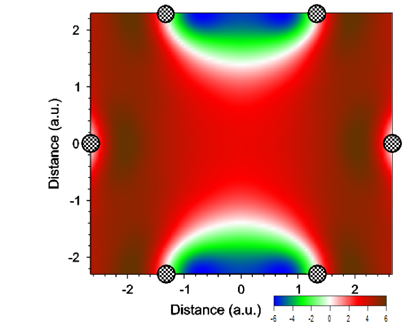
Figure 3: (color online) Real (left) and imaginary (right) parts of the wave function (in arbitrary units) at the $z=0$ plane for the third lowest band at $K$ point.

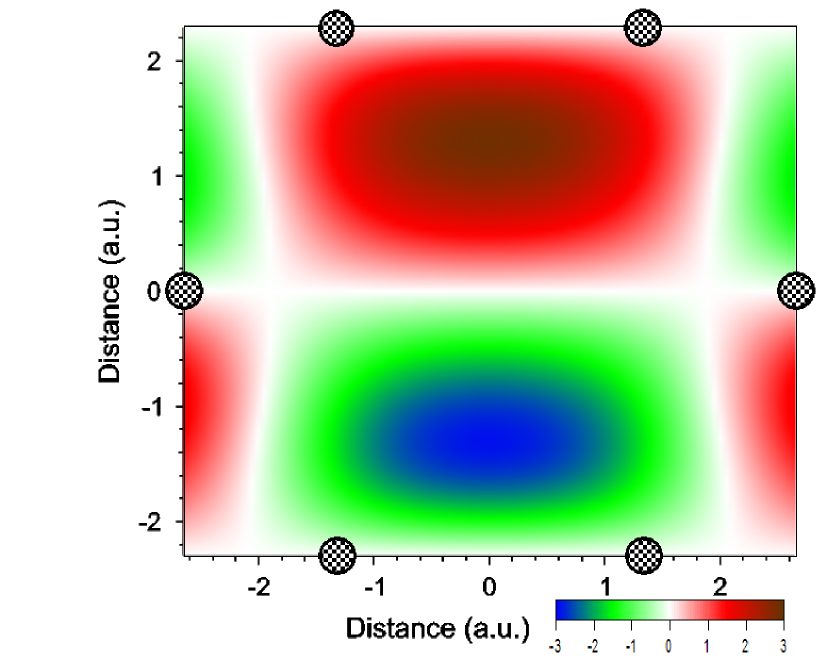
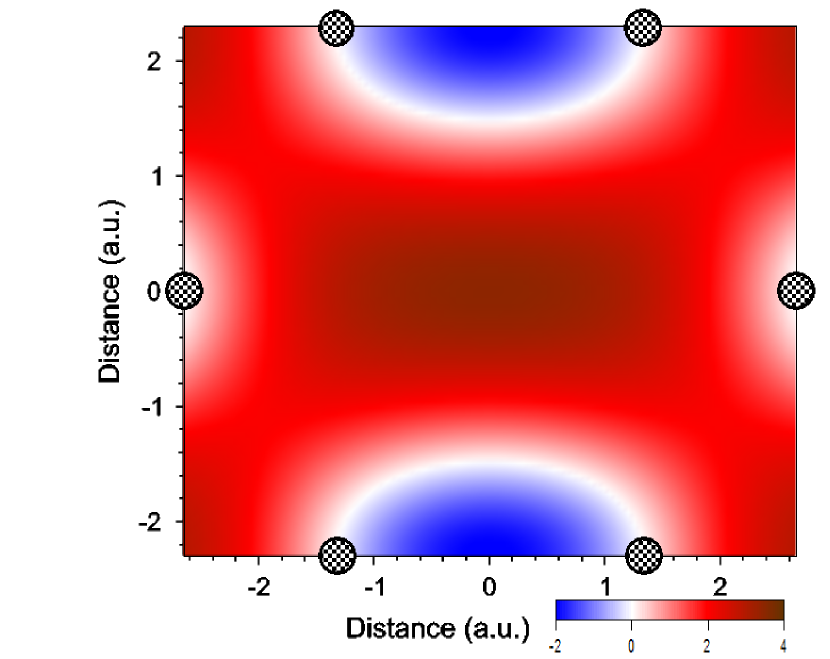
Figure 4: (color online) Real (left) and imaginary (right) parts of the wave function (in arbitrary units) at the $z=1$ a.u. plane for the sixth lowest band at $K$ point.

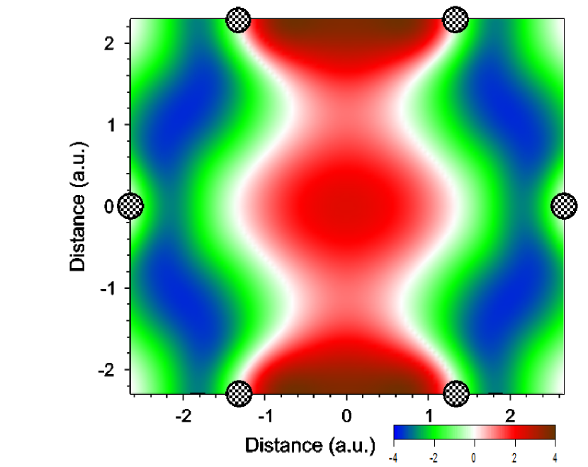
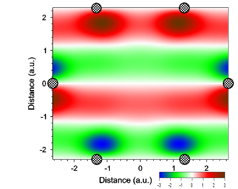
Figure 5: (color online) Real (left) and imaginary (right) parts of the wave function (in arbitrary units) at the $z=0$ plane for the ninth lowest band at $K$ point.

In our previous publication kogan1 we presented simple TBM interpretation of the degeneracy of the $\pi$ bands at the point $K$ ($E^{\prime\prime}$ representation). The general TBM Hamiltonian for the $\pi$ bands is

$$H=-\left(\begin{array}[]{cc}E_{p}+\sum_{\bf a}t^{\prime}({\bf a})e^{i{\bf k\cdot a}}&\sum_{\bf a}t({\bf a}+{\bf\delta})e^{i{\bf k\cdot}({\bf a}+{\bf\delta})}\\ \sum_{\bf a}t^{*}({\bf a}+{\bf\delta})e^{-i{\bf k\cdot}({\bf a}+{\bf\delta})}&E_{p}+\sum_{\bf a}t^{\prime}({\bf a})e^{i{\bf k\cdot a}}\end{array}\right),$$ (15)

where $E_{p}$ is the energy of an isolated $|p_{z}>$ orbital, ${\bf a}$ is an arbitrary lattice vector. The structure of graphene can be seen as a triangular lattice with a basis of two atoms per unit cell, displaced from each other by any one (fixed) vector $\delta$ connecting two sites of different sub-lattices. From Ref. neto we get that ${\bf a}$ is a linear combination of ${\bf a}_{1}=\frac{a}{2}\left(3,\sqrt{3}\right)$, ${\bf a}_{2}=\frac{a}{2}\left(3,-\sqrt{3}\right)$ and ${\bf\delta}$ can be chosen as ${\bf\delta}=-a\left(1,0\right)$. Also $K=\frac{2\pi}{3a}\left(1,\frac{1}{\sqrt{3}}\right)$.

Consider, for example, three terms in the sum $\sum_{\bf a}t({\bf a}+{\bf\delta})e^{i{\bf k\cdot}({\bf a}+{\bf\delta})}$ corresponding to hopping between the nearest neighbours. The hopping integral $t({\bf a}+{\bf\delta})$ is the same for all three terms; the multiplier $e^{i{\bf k\cdot}({\bf a}+{\bf\delta})}$ takes three values: $1,e^{2\pi i/3},e^{-2\pi i/3}$, $\epsilon=e^{2\pi i/3}$. Hence, due to the identity $1+e^{2\pi i/3}+e^{-2\pi i/3}=0$, the non-diagonal terms in the Hamiltonian (15) disappear; hence degeneracy of the bands.

Similar interpretation can be supplied for the degeneracy of the $\sigma$ bands at the K point. The reasoning from the previous paragraph can be repeated verbatim for the $E^{\prime}$ representation realized by $\psi^{A}_{s}$ and $\psi^{B}_{s}$ functions. The TBM analysis of the representations realized by $\psi^{A,B}_{p_{x,y},}$ functions is a bit more complicated.

Let us start defining a convenient for our purpose basis for the $E$ representation of the group $C_{3v}$ realized by $|p_{x,y}>$ orbitals:

$$|p_{L}>=|p_{x}>+\epsilon\hat{T}|p_{x}>+\epsilon^{2}\hat{T}^{2}|p_{x}>$$

$$|p_{R}>=|p_{x}>+\epsilon^{2}\hat{T}|p_{x}>+\epsilon\hat{T}^{2}|p_{x}>,$$ (17)

where $\hat{T}$ is an operator of rotation by the angle $2\pi/3$. If we graphically present $|p_{x}>$ orbital by a line in the $x$-direction, then the basis vectors can be presented as two stars.

\begin{picture}(6.0,6.0)\par\put(2.0,3.0){ \line(-1,-2){1.0}} \put(2.0,3.0){ \line(-1,2){1.0}} \put(2.0,3.0){ \line(1,0){2.3}} \put(2.0,4.0){$\epsilon$} \put(3.5,3.2){$1$} \put(2.0,1.5){$\epsilon^{2}$} \par\put(8.0,3.0){ \line(-1,-2){1.0}} \put(8.0,3.0){ \line(-1,2){1.0}} \put(8.0,3.0){ \line(1,0){2.3}} \put(9.5,3.2){$1$} \put(8.0,4.0){$\epsilon^{2}$} \put(8.0,1.5){$\epsilon$} \par\end{picture}

It is obvious that rotation of each basis vector by $2\pi/3$ just multiplies it by $\epsilon$ ($\epsilon^{2}$).

Returning to our original representation we chose the basis vectors as

$$\begin{array}[]{l}\psi_{1}\equiv\psi^{A}_{L}=\sum_{{\bf R}_{A}}e^{i{\bf K\cdot R}_{A}}|p_{L}>_{{\bf R}_{A}}\\ \psi_{2}\equiv\psi^{A}_{R}=\sum_{{\bf R}_{A}}e^{i{\bf k\cdot R}_{A}}|p_{R}>_{{\bf R}_{A}}\\ \psi_{3}\equiv\psi^{B}_{L}=\sum_{{\bf R}_{B}}e^{i{\bf k\cdot R}_{B}}|p_{R}>_{{\bf R}_{B}}\\ \psi_{4}\equiv\psi^{B}_{R}=\sum_{{\bf R}_{B}}e^{i{\bf k\cdot R}_{B}}|p_{R}>_{{\bf R}_{B}},\end{array}$$ (22)

where $|\dots>_{\bf R}$ means an orbital centered at the site ${\bf R}$. The Hamiltonian matrix in such basis has the form

$$H=\left(\begin{array}[]{cccc}0&\dots&0&\dots\\ \dots&0&\dots&0\\ 0&\dots&0&\dots\\ \dots&0&\dots&0\\ \end{array}\right),$$ (27)

where we have shifted energy to $H_{11}+E_{p}$ ($E_{p}$ is the energy of an isolated $|p>$ orbital). The elements indicated by three dots are of no interest to us. The origin of zeros on the diagonal of the matrix is obvious. To understand presence of non-diagonal zeros (in a chosen basis) consider, for example, the three terms in the $H_{13}$ matrix element corresponding to hopping between the nearest neighbours. They can be graphically presented as

\begin{picture}(12.0,16.0)\par\put(13.0,8.0){ \line(-1,-2){1.0}} \put(13.0,8.0){ \line(-1,2){1.0}} \put(13.0,8.0){ \line(1,0){2.3}} \put(14.5,8.2){$1$} \put(13.0,9.0){$\epsilon$} \put(13.0,6.5){$\epsilon^{2}$} \par\put(18.0,8.0){ \line(-1,-2){1.0}} \put(18.0,8.0){ \line(-1,2){1.0}} \put(18.0,8.0){ \line(1,0){2.3}} \put(19.5,8.2){$1$} \put(18.0,9.0){$\epsilon$} \put(18.0,6.5){$\epsilon^{2}$} \par\put(10.5,13.0){ \line(-1,-2){1.0}} \put(10.5,13.0){ \line(-1,2){1.0}} \put(10.5,13.0){ \line(1,0){2.3}} \put(12.0,13.2){$\epsilon$} \put(10.5,14.0){$\epsilon^{2}$} \put(10.5,11.5){$1$} \par\put(10.5,3.0){ \line(-1,-2){1.0}} \put(10.5,3.0){ \line(-1,2){1.0}} \put(10.5,3.0){ \line(1,0){2.3}} \put(12.0,3.2){$\epsilon^{2}$} \put(10.5,4.0){$1$} \put(10.5,1.5){$\epsilon$} \par\par\end{picture}

Again, the identity $1+e^{2\pi i/3}+e^{-2\pi i/3}=0$ leads to the disappearance of the matrix element. The structure of the matrix (27) shows that its eigenvalues can be grouped into pairs with the the same modulus and the opposite signs. On the other hand, this structure shows that the product of all eigenvalues is equal to zero. Hence degeneracy of the bands at the energy $0$ (that is at the energy $H_{11}+E_{p}$).

III.3 $M$ - point

Finally consider the point $M$. The functions $\psi_{\bf M}^{j}$ realize $A_{g}+B_{3u}$ representation of the group $D_{2h}$. The orbitals $|s>$, $|p_{z}>$, $|p_{x}>$ and $|p_{y}>$ realize $A_{g}$, $B_{1u}$, $B_{3u}$ and $B_{2u}$ representations respectively. Thus the identity

$$(A_{g}+B_{3u})\times B_{1u}=B_{1u}+B_{2g}$$ (28)

shows the symmetry of the two $\pi$ bands at the point $M$; the identity

$$(A_{g}+B_{3u})\times B_{2u}=B_{2u}+B_{1g}$$ (29)

shows the symmetry of the two $\sigma$ bands constructed from $|p_{y}>$ orbitals, and the identities

$$\begin{array}[]{l}(A_{g}+B_{3u})\times B_{3u}=B_{3u}+A_{g}\\ (A_{g}+B_{3u})\times A_{g}=A_{g}+B_{3u}\end{array}$$ (32)

show that there are two $A_{g}$ and two $B_{3u}$ bands constructed from $|p_{x}>$ and $|s>$ orbitals.

From analyzing the TBM neto we come to the conclusion that the band $B_{1u}$ lies above the band $B_{2g}$. From Eq. (32) we come to the conclusion that, if overlapping between $|p_{x}>$ orbitals is stronger than that between $|s>$ orbitals, the lowest band at the point $M$ realizes $B_{3u}$ reprezentation.

On Figs. 6 -10 we present the results of the calculations of the wave functions of the occupied and the lowest unoccupied bands at the point $M$. The wave functions of the $\sigma$ bands are plotted at the plane $z=0$. For the $\pi$ bands, the wave function is identically equal to zero at the $z=0$ plane, so we plotted the wave function at the plane $z=1$ a.u.

For the lowest (at the point $M$) band the wave function is equal to zero along the $y$ - axis, which corresponds to the representation $B_{3u}$. (Because the wave function is antisymmetric with respect to reflection, it should be equal to zero at the axis of reflection.) The wave function of the next band is different from zero everywhere at the plane, which is consistent with the representation $A_{g}$. The wave function of the third band is equal to zero at the $x$ -axis, which corresponds to the representation $B_{2u}$.

For the forth band the wave function is equal to zero along the $y$ - axis, which corresponds to the representation $B_{2g}$. The wave function of the first unoccupied band is different from zero everywhere at the plane $z=1$ a.u., which is consistent with the representation $B_{1u}$.

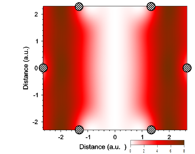
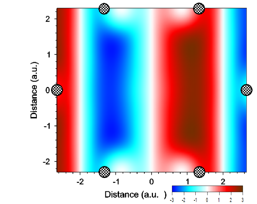
Figure 6: (color online) Real (left) and imaginary (right) parts of the wave function (in arbitrary units) at the $z=0$ plane for the lowest band at $M$ point.

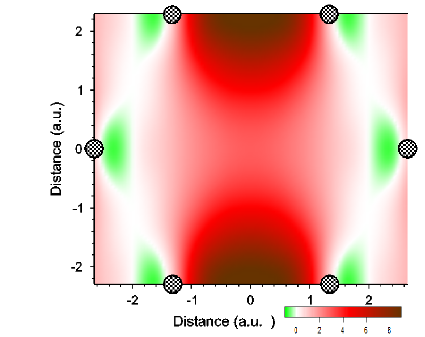
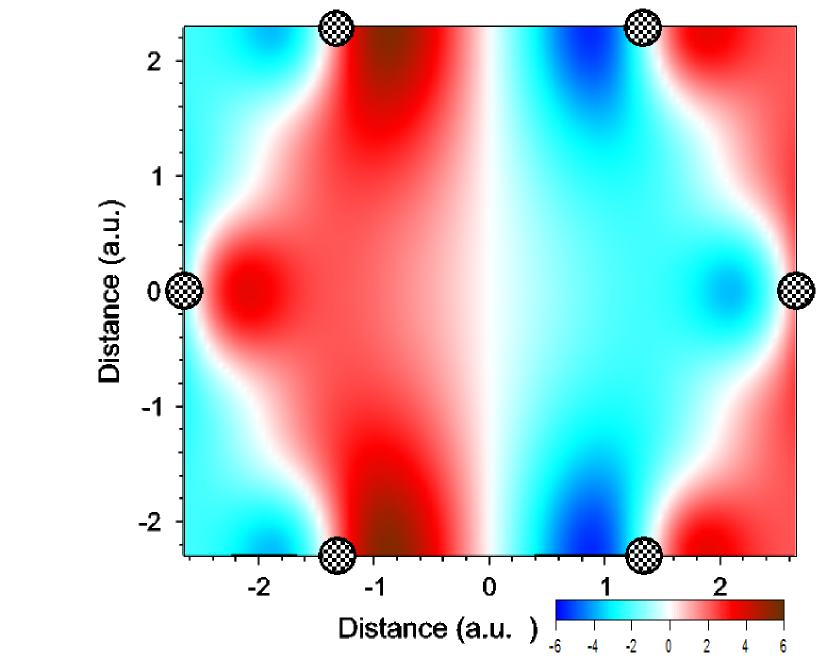
Figure 7: (color online) Real (left) and imaginary (right) parts of the wave function (in arbitrary units) at the $z=0$ plane for the second lowest band at $M$ point.

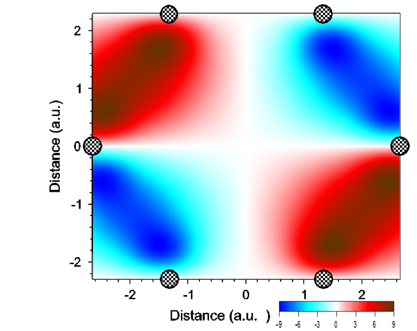
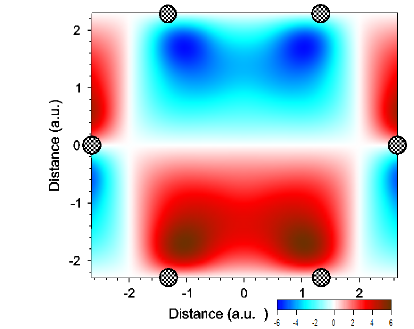
Figure 8: (color online) Real (left) and imaginary (right) parts of the wave function (in arbitrary units) at the $z=0$ plane for the third lowest band at $M$ point.

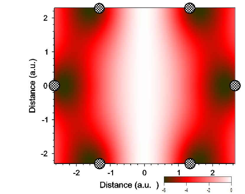
Figure 9: (color online) Real (left) and imaginary (right) parts of the wave function (in arbitrary units) at the $z=1$ a.u. plane for the forth lowest band at $M$ point.

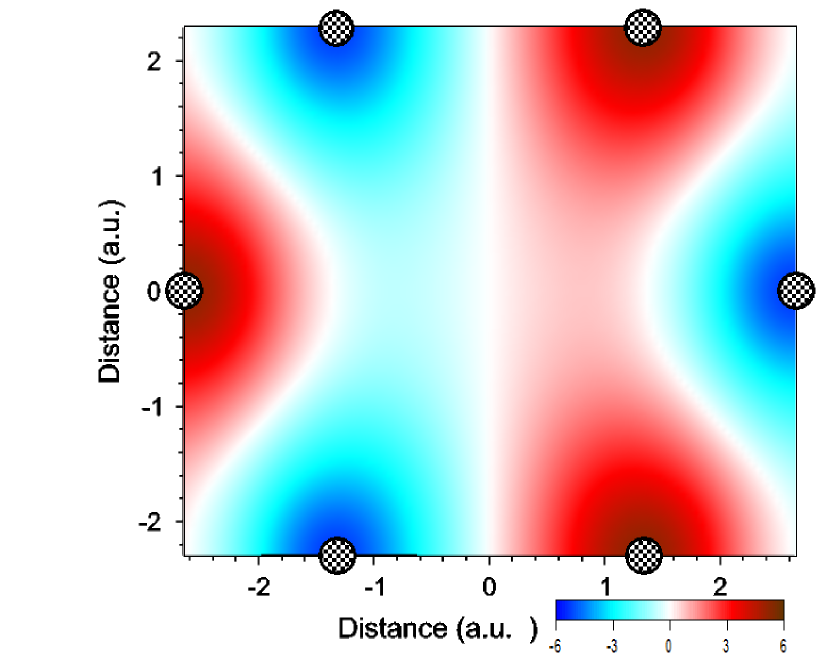
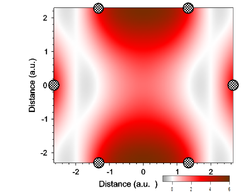
Figure 10: (color online) Real (left) and imaginary (right) parts of the wave function (in arbitrary units) at the $z=1$ a.u. plane for the fifth lowest band at $M$ point.

III.4 $\Gamma-K-M$ - lines

The symmetry of the band(s) at the symmetry point determines the symmetry of the band(s) at the symmetry lines containing this point landau ; thomsen . At the line $\Gamma-K-M$ the functions $\phi_{\bf k}^{A,B}$ realize $A_{1}+B_{1}$ representation of the group $C_{2v}$. The orbital $|p_{z}>$ realizes $B_{2}$ representation. From the identities $B_{2}\times A_{1}=B_{2}$, $B_{2}\times B_{1}=A_{2}$ we come to the conclusion that the lower band should realize $B_{2}$ representation. At the line $\Gamma-M$ the functions $\phi_{\bf k}^{A,B}$ realize twice $A_{1}$ representation of the group $C_{2v}$. The orbital $|p_{z}>$ generalizes $B_{2}$ representation. From the identity $B_{2}\times A_{1}=B_{2}$ we obtain that both $\pi$ bands realize $B_{2}$ representation.

IV Appendix

For convenience of the reader in we reproduce character tables for the groups used in the paper landau (Tables 1 and 2).

$C_{2v}$		$E$	$C_{2}$	$\sigma_{v}$	$\sigma_{v}^{\prime}$
	$D_{2}$	$E$	$C_{2}^{z}$	$C_{2}^{y}$	$C_{2}^{x}$
$A_{1};z$	$A$	$1$	1	1	1
$B_{2};y$	$B_{3};x$	$1$	$-1$	$-1$	1
$A_{2}$	$B_{1};z$	$1$	1	$-1$	$-1$
$B_{1};x$	$B_{2};y$	$1$	$-1$	1	$-1$

Table 1: Character table for irreducible representations of $C_{2v}$ and $D_{2}$ point groups

$D_{6}$		$E$	$C_{2}$	$2C_{3}$	$2C_{6}$	$3U_{2}$	$3U_{2}^{\prime}$
	$D_{3h}$	$E$	$\sigma$	$2C_{3}$	$2S_{3}$	$3U_{2}$	$3\sigma_{v}$
$A_{1}$	$A_{1}^{\prime}$	1	1	1	1	1	1
$A_{2}$	$A_{2}^{\prime}$	1	1	1	1	$-1$	$-1$
$B_{1}$	$A_{1}^{\prime\prime}$	1	$-1$	1	$-1$	1	$-1$
$B_{2}$	$A_{2}^{\prime\prime}$	1	$-1$	1	$-1$	$-1$	1
$E_{2}$	$E^{\prime}$	2	2	$-1$	$-1$	0	0
$E_{1}$	$E^{\prime\prime}$	2	$-2$	$-1$	1	0	0

Table 2: Character table for irreducible representations of $D_{6}$ and $D_{3h}$ point groups

The characters of the groups $D_{2h}$ and $D_{6h}$ are obtained using the relations $D_{2h}=D_{2}\times C_{i}$ and $D_{6h}=D_{6}\times C_{i}$, where $C_{i}$ is the inversion group.

References

- (1) W. M. Lomer, Proc. R. Soc. London, Ser. A 227, 330 (1955).
- (2) J. C. Slonczewski and P. R. Weiss, Phys. Rev. 109, 272 (1958).
- (3) G. Dresselhaus and M. S. Dresselhaus, Phys. Rev. 140, A401 (1965).
- (4) F. Bassani and G. Pastori Parravicini, Nuovo Cimento B 50, 95 (1967).
- (5) L. M. Malard, M. H. D. Guimaraes, D. L. Mafra, M. S. C. Mazzoni, and A. Jorio, Phys. Rev. B 79, 125426 (2009).
- (6) J. L. Manes, Phys. Rev. B 85, 155118 (2012).
- (7) F. Hund and B. Mrowka, Sachs. Akad. Wiss., Leipzig 87, 325 (1935).
- (8) E. Kogan, V. U. Nazarov, V. M. Silkin, and M. Kaveh, Phys. Rev. B 89, 165430 (2014).
- (9) M. Posternak, A. Baldereschi, A. J. Freeman, E. Wimmer, and M. Weinert, Phys. Rev. Lett. 50, 761 (1983).
- (10) M. Posternak, A. Baldereschi, A. J. Freeman, and E. Wimmer, Phys. Rev. Lett. 52, 863 (1984).
- (11) T. O. Wehling, I. Grigorenko, A. I. Lichtenstein, and A. V. Balatsky, Phys. Rev. Lett. 101, 216803 (2008).
- (12) V. M. Silkin, J. Zhao, F. Guinea, E. V. Chulkov, P. M. Echenique, and H. Petek, Phys. Rev. B 80, 121408(R) (2009).
- (13) P. M. Echenique and J. B. Pendry, J. Phys. C 11, 2065 (1978).
- (14) S. G. Davison and M. Stȩślicka, Basic Theory of Surface States, (Oxford University Press, Oxford, 1992).
- (15) T. Fauster, C. Reuss, I. L. Shumay, and M. Weinelt, Chem. Phys. 251, 111 (2000).
- (16) P. M. Echenique, R. Berndt, E. V. Chulkov, Th. fauster, A. Goldmann, and U. Höfer, Surf. Sci. Rep. 52, 219 (2004).
- (17) B. Borca, S. Barja, M. Garnica, D. Sanchez-Portal, V. M. Silkin, E. V. Chulkov C. F. Hermans, J. J. Hinarejos, A. L. Vazquez de Parga, A. Arnau, P. M. Echenqiue, and R. Miranda, Phys. Rev. Lett. 105, 036804 (2010).
- (18) H. G. Zhang, H. Hu, Y. Pan, J. H. Mao, M. Gao, H. M. Guo, S. X. Du, T. Greber, and H.-J. Gao, J. Phys.: Condens. Matter 22, 302001 (2010).
- (19) D. Niesner, T. Fauster, J. I. Dadap, N. Zaki, K. R. Knox, P.-C. Yeh, R. Bhandari, R. M. Osgood, M. Petrović, and M. Kralj, Phys. Rev. B 85, 081402(R) (2012).
- (20) N. Atmbrust, J. Güdde, P. Jacob, and U. Höfer, Phys. Rev. Lett. 108, 056801 (2012).
- (21) D. Nobis, M. Potenz, D. Niesner, and T. Fauster, Phys. Rev. B 89, 195435 (2013).
- (22) F. Craes, S. Runte, J. Klinkhammer, M. Kralj, T. Michely, and C. Busse, Phys. Rev. Lett. 111, 056804 (2013).
- (23) D. Niesner and T. Fauster, J. Phys.: Condens. Matter 26, 393001 (2014).
- (24) S. Bose, V. M. Silkin, R. Ohmann, I. Brihuega, L. Vitali, C. H. Michaelis, P. Mallet, J. Y. Veuillen, M. A. Schneider, E. V. Chulkov, P. M. Echenique, and K. Kern, New J. Phys. 12, 023028 (2010).
- (25) K. Takahashi, M. Imamura, I. Yamamoto, J. Azuma, and M. Kamada, Phys. Rev. B 89, 155303 (2014).
- (26) A. J. Shearer, J. E. Johns, B. W. Caplins, D. E. Suich, M. C. Hersam, and C. B. Harris, Appl. Phys. Lett. 104, 231604 (2014).
- (27) M. Feng, J. Zhao, and H. Petek, Science 320, 359 (2008).
- (28) J. Zhao, M. Feng, J. Yang, and H. Petek, ACS Nano 3, 853 (2009).
- (29) T. Fauster, F. J. Himpsel, J. E. Fischer, and E. W. Plummer, Phys. Rev. Lett. 51, 430 (1983).
- (30) V. N. Strocov, P. Blaha, H. I Starnberg, M. Rohlfing, R. Claessen, J.-M. Debever, and J.-M. Themlin, Phys. Rev. B 61, 4994 (2000).
- (31) G. Csányi, P. B. Littlewood, A. H. Nevidomskyy, C. J. Pickard, and B. D. Simons, Nat. Phys. 1, 42 (2005).
- (32) P. M. Coelho, D. D. dos Reis, M. J. S. Matos, T. G. Mendes-de-Sa, A. M. B. Goncalves, R. G. Lacerda, A. Malachias, and R. Magalhaes-Paniago, Surf. Sci. 644, 135 (2016).
- (33) V. U. Nazarov, E. E. Krasovskii, and V. M. Silkin, Phys. Rev. B, 87, 041405(R) (2013).
- (34) F. Wicki, J.-N. Longchamp, T. Latychevskaia, C. Escher, and H.-W. Fink, Phys. Rev. B 94, 075424 (2016).
- (35) M. S. Dresselhaus, G. Dresselhaus, A. Jorio, Group theory: Application to the physics of condenced matter, (Springer-Verlag Berlin Heidelberg, 2008).
- (36) C. Thomsen, S. Reich, J. Maultzsch, Carbon Nanotubes: Basic Concepts and Physical Properties, (Wiley Online Library, 2004 WILEY-VCH Verlag GmbH).
- (37) L. D. Landau and E. M. Lifshitz, Landau and Lifshitz Course of Theoretical Physics: Vol. 3 Quantum Mechanics, (Pergamon Press, 1991).
- (38) A. H. Castro Neto, F. Guinea, N. M. R. Peres, K. S. Novoselov and A. K. Geim, Rev. Mod. Phys. 81, 109 (2009).
- (39) C. Kittel, Quantum Theory of Solids, (John Willey & Sons. Inc., New York - London, 1963).
- (40) E. Kogan and V. U. Nazarov, Phys. Rev. B 85, 115418 (2012).