Next-to-leading order corrections to the spin-dependent energy spectrum of hadrons from polarized top quark decay in the general two Higgs doublet model

Abstract

In recent years, searches for the light and heavy charged Higgs bosons have been done by the ATLAS and the CMS collaborations at the Large Hadron Collider (LHC) in proton-proton collision. Nevertheless, a definitive search is a program that still has to be carried out at the LHC. The experimental observation of charged Higgs bosons would indicate physics beyond the Standard Model. In the present work, we study the scaled-energy distribution of bottom-flavored mesons ($B$) inclusively produced in polarized top quark decays into a light charged Higgs boson and a massless bottom quark at next-to-leading order in the two-Higgs-doublet model; $t(\uparrow)\to bH^{+}\to BH^{+}+X$. This spin-dependent energy distribution is studied in a specific helicity coordinate system where the polarization vector of the top quark is measured with respect to the direction of the Higgs momentum. The study of these energy distributions could be considered as a new channel to search for the charged Higgs bosons at the LHC. For our numerical analysis and phenomenological predictions, we restrict ourselves to the unexcluded regions of the MSSM $m_{H^{+}}-\tan\beta$ parameter space determined by the recent results of the CMS CMS:2014cdp and ATLAS TheATLAScollaboration:2013wia collaborations.

I Introduction

The electroweak symmetry breaking in the standard model (SM) of particle physics is described with the Higgs mechanism. In 2012, the SM Higgs boson with a mass of approximately $125$ GeV was discovered by the CMS and ATLAS experiments Aad:2012tfa ; Chatrchyan:2012xdj at the CERN Large Hadron Collider (LHC). Although the current LHC Higgs data are consistent with the SM, there is still the possibility that the observed Higgs state could be part of a model with an extended Higgs sector. Models including an extended Higgs sector are constrained by the measured mass, charge-parity (CP) quantum numbers, and production rates of the new boson. The discovery of another heavy scalar boson, neutral or charged, would clearly represent unambiguous evidence for the presence of new physics beyond the standard model.

Charged Higgs bosons are predicted in models with at least two Higgs doublets. The simplest of such models is known as the two-Higgs-doublet model (2HDM) Lee:1973iz where the Higgs sector of the SM is extended, typically by adding an extra doublet of complex Higgs fields. After spontaneous symmetry breaking, the particle spectrum of this model includes five physical Higgs bosons: light and heavy CP-even Higgs bosons h and H with $m_{h}<m_{H}$, a CP-odd Higgs boson A, plus two charged Higgs bosons $H^{\pm}$ Djouadi:2005gj . The production mechanisms and decay modes of charged Higgs bosons depend on their masses, $m_{H^{\pm}}$. At hadron colliders, a charged Higgs boson can be produced through several channels. For light charged Higgs bosons that their masses are smaller than the difference between the mass of top ($m_{t}$) and the bottom quark ($m_{b}$), $m_{H^{\pm}}<m_{t}-m_{b}$, the primary production mechanism is through the decay of a top quark $t\to bH^{+}$ Gunion . Then, in this case, the light charged Higgs bosons are produced most frequently via $t\bar{t}$ production. At the LHC, one expects a cross section $\sigma(pp\to t\bar{t}X)\approx 1$ (nb) at design energy $\sqrt{S}=14$ TeV Langenfeld:2009tc . With the LHC design luminosity of $10^{34}cm^{-2}s^{-1}$ in each of the four experiments, it is expected to produce a $t\bar{t}$ pair per second. Thus, the LHC is a superlative top factory which allows one to search for the charged Higgs boson in the subsequent decay products of the top pairs $t\bar{t}\rightarrow H^{\pm}H^{\mp}b\bar{b}$ and $t\bar{t}\rightarrow H^{\pm}W^{\mp}b\bar{b}$ when $H^{\pm}$ decays into $\tau$ lepton and neutrino. See also Ref. Aoki:2011wd for a review of all available production modes of light charged Higgs bosons at the LHC in 2HDMs.

The Large Electron-Positron (LEP) collider experiments have determined a model independent low limit of 78.6 GeV on the charged Higgs mass Heister:2002ev ; Abdallah:2003wd ; Achard:2003gt ; Abbiendi:2008aa at a $95\%$ confidence level. The most sensitive $95\%$ confidence level upper limits on the branching fraction $B(t\to bH^{+})$ have been determined by the ATLAS and CMS experiments for the mass range $m_{H^{+}}=80-160$ GeV. More details can also be found in Khachatryan:2015qxa . We shall discuss about the recent results on a search for a charged Higgs boson by the CMS CMS:2014cdp and ATLAS TheATLAScollaboration:2013wia collaborations in Sec. III.

The primary purpose of this paper is the evaluation of the next-to-leading order (NLO) QCD corrections to the differential partial decay width ($d\Gamma/dx_{i}$) of a top quark into a charged Higgs boson and a bottom quark, $t\to bH^{+}$, where $x_{i}$ stands for the scaled-energy fraction of the b-quark or the gluon emitted at NLO (see Eq. (8)). These differential decay widths, which are presented for the first time, are needed to obtain the energy spectrum of B-mesons through top decays. More detail will be discussed in Sec. III.
The $\alpha_{s}$-order corrections to the top quark decay width, $\Gamma(t\to bH^{+})$, were previously computed in kadeer for the polarized top quark and in Ali:2009sm ; Czarnecki ; Liud ; Li:1990cp for the unpolarized one. In MoosaviNejad:2011yp , we calculated the unpolarized differential decay width $d\Gamma(t\to bH^{+})/dx_{b}$ and showed that our result after integration over $x_{b}$ ($0\leq x_{b}\leq 1$) is in complete agreement with Refs. Ali:2009sm ; Czarnecki ; Liud and the corrected version of Li:1990cp . In the present work, to ensure our calculations we check that our result for the polarized differential decay width $d\Gamma(t(\uparrow)\to bH^{+})/dx_{b}$ is in complete agreement with the result presented in kadeer for the polarized decay width $\Gamma(t(\uparrow)\to bH^{+})$, if one integrates over $x_{b}$, i.e. $\Gamma=\int_{0}^{1}dx_{b}d\Gamma(t(\uparrow)\to bH^{+})/dx_{b}$.

On the other hand, the b-quark produced from the top quark decay hadronizes before it decays, therefore each b-jet contains a bottom-flavored hadron which most of the times is a B-meson, $b\to B+X$. Therefore, the decay process $t\to bH^{+}(+g)\to BH^{+}+X$ is of prime importance and it is an urgent task to predict its partial decay width ($d\Gamma/dx_{B}$) as reliably as possible. In fact, one of the proposed ways to search for the charged Higgs bosons at the LHC is the study of the energy distribution of B-mesons inclusively produced in the polarized/unpolarized top quark decays. In Ref. MoosaviNejad:2011yp , we studied the energy spectrum of the bottom-flavored mesons in unpolarized top quark decays into a charged-Higgs boson and a massless bottom quark at NLO in the 2HDM. In the present work we study the energy distribution of B-meson produced through the polarized top decay $t(\uparrow)\to BH^{+}+X$ at NLO, and compare it to the unpolarized one. For our numerical analysis and our phenomenological predictions, we restrict ourselves to the unexcluded regions of the $m_{H^{+}}-\tan\beta$ parameter space determined by the recent results of the CMS CMS:2014cdp and ATLAS TheATLAScollaboration:2013wia collaborations.
The top quark polarization can be studied by the angular correlations between the top spin and its decay product momenta so that these spin-momentum correlations will enable us to detailed study of the top decay mechanism.

Since, highly polarized top quarks will become available at hadron colliders through single top production, at the $33\%$ level of the top pair production rate Mahlon:1996pn ; Espriu:2002wx , and also at future $e^{+}e^{-}$ colliders these measurements of the decay rates will be important to future tests of the Higgs coupling in the minimal supersymmetric SM (MSSM).

This paper is organized as follows. In Sec. II, we present our analytical results of the ${\cal O}(\alpha_{s})$ QCD corrections to the tree-level rate of $t(\uparrow)\rightarrow bH^{+}$. We work in the massless scheme where the b-quark mass is neglected from the beginning but the arbitrary value of $m_{H^{+}}$ is retained. In Sec. III, we present our numerical analysis of inclusive production of a meson from polarized top quark decay considering the factorization theorem and DGLAP equations. We shall compare our result with the one from the unpolarized top decay. In Sec. IV, our conclusions are summarized.

II Parton level results in the general two Higgs doublet model

In this section, assuming the condition $m_{t}>m_{b}+m_{H^{+}}$ we study the NLO radiative corrections to the partial decay width

$$t(\uparrow)\rightarrow b+H^{+},$$ (1)

in the general 2HDM, where $H_{1}$ and $H_{2}$ are the doublets whose vacuum expectation values respectively give masses to the down and up type quarks. If we label the vacuum expectation values of the fields $H_{1}$ and $H_{2}$ as $\textbf{v}_{1}$ and $\textbf{v}_{2}$, respectively, one has $\textbf{v}_{1}^{2}+\textbf{v}_{2}^{2}=(\sqrt{2}G_{F})^{-1}$ where $G_{F}$ is the Fermi’s constant. The ratio of the two values $\textbf{v}_{1}$ and $\textbf{v}_{2}$ is a free parameter and one can define the angle $\beta$ to parametrize it, i.e. $\tan\beta=\textbf{v}_{2}/\textbf{v}_{1}$. Also, a linear combination of the charged components of $H_{1}$ and $H_{2}$ gives the observable charged Higgs $H^{\pm}$, i.e. $H^{\pm}=H_{2}^{\pm}\cos\beta-H_{1}^{\pm}\sin\beta$.
In a general two Higgs doublet model, in order to avoid a tree-level flavor-changing neutral currents, the generic Higgs coupling to all quarks should be restricted. In fact, one should not couple the same Higgs doublet to up- and down-type quarks simultaneously. Therefore, we limit ourselves to specific models which naturally stop these problems by restricting the Higgs coupling. There are, then, two possibilities (two models) for the two Higgs doublets to couple to the fermions.
In model 1 (first possibility), one of the Higgs doublets ($H_{1}$) couples to all bosons and the remaining doublet $H_{2}$ couples to all the quarks. In this model, the Yukawa couplings between the top quark, the bottom quark and the charged Higgs boson are given by GHK

$$L_{1} = \frac{g_{{}_{W}}}{2\sqrt{2}m_{W}}V_{tb}\cot\beta\bigg{\{}H^{+}\bar{t}\big{[}m_{t}(1-\gamma_{5})-$$ (2)

$$m_{b}(1+\gamma_{5})\big{]}b\bigg{\}}+H.c,$$

where the weak coupling factor $g_{W}$ is related to the Fermi coupling constant by $g_{W}^{2}=4\sqrt{2}m_{W}^{2}G_{F}$ and $V_{tb}\approx 1$ is the 33 entry of the CKM matrix.

In model 2 (second possibility), the doublet $H_{1}$ couples to the right-handed down-type quarks and the $H_{2}$ couples to the right-handed up-type quarks ($u_{R},c_{R},t_{R}$). In model 2, the interaction Lagrangian leads to an $H^{+}b\bar{t}$ vertex as

$$L_{2} = \frac{g_{{}_{W}}}{2\sqrt{2}m_{W}}V_{tb}\bigg{\{}H^{+}\bar{t}\big{[}m_{t}\cot\beta(1-\gamma_{5})+$$ (3)

$$m_{b}\tan\beta(1+\gamma_{5})\big{]}b\bigg{\}}+H.c.$$

These models are often known as Type-I and Type-II 2HDM scenarios. The MSSM Fayet:1974pd ; Fayet:1976et ; Fayet:1977yc ; Dimopoulos:1981zb is a special case of a Type-II 2HDM scenario.
Note that, in type-II 2HDM there is a charged Higgs mass lower limit of $m_{H}\approx 480$ GeV at $95\%$ confidence level (CL)Misiak:2015xwa . However, this limit is not imposed on a supersymmetric version of type-II (e.g. MSSM). Therefore in this paper, we work on type-I or MSSM as a type-II model.

Generally, the dynamics of the current-induced $t\rightarrow b$ transition is embodied in the following hadron tensor

$$H^{\mu\nu} \propto\sum_{X_{b}}\int d\Pi_{f}\delta^{4}(p_{t}-p_{{}_{H^{+}}}-p_{{}_{X_{b}}})$$

$$\times<t(p_{t},s_{t})|J^{\nu{\dagger}}|X_{b}><X_{b}|J^{\mu}|t(p_{t},s_{t})>,$$

where $d\Pi_{f}$ refers to the Lorentz-invariant phase space factor and $s_{t}$ stands for the top quark spin. At NLO approximation, we consider only two types of intermediate states in Eq. (II), i.e., $|X_{b}>=|b>$ for the Born level term and ${\cal O}(\alpha_{s})$ one-loop contributions and $|X_{b}>=|b+g>$ for the ${\cal O}(\alpha_{s})$ tree graph contribution. In the SM, the weak current is given by $J^{\mu}\propto\bar{\psi}_{b}\gamma^{\mu}(1-\gamma_{5})\bar{\psi}_{t}$ while in the 2HDM, considering the interaction Lagrangians (2) and (3) the current is expressed as $J^{\mu}\propto\bar{\psi}_{b}(a+b\gamma_{5})\bar{\psi}_{t}$ in which the coupling factors are

$$\textbf{model 1}:\quad a = \frac{g_{{}_{W}}}{2\sqrt{2}m_{W}}V_{tb}(m_{t}-m_{b})\cot\beta,$$

$$b = \frac{g_{{}_{W}}}{2\sqrt{2}m_{W}}V_{tb}(m_{t}+m_{b})\cot\beta,$$ (5)

or

$$\textbf{model 2}:\quad a = \frac{g_{{}_{W}}}{2\sqrt{2}m_{W}}V_{tb}(m_{t}\cot\beta+m_{b}\tan\beta),$$

$$b = \frac{g_{{}_{W}}}{2\sqrt{2}m_{W}}V_{tb}(m_{t}\cot\beta-m_{b}\tan\beta).$$

The decay process (1) is analyzed in the rest frame of the top quark where the three-momentum $\vec{P}_{H}$ of the $H^{+}$ boson points into the direction of the positive $z$-axis and the polar angle $\theta_{P}$ is defined as the angle between the polarization vector $\vec{P}_{t}$ of the top quark and the $z$-axis (see Fig. 1). Here, we follow the notation of Ref. MoosaviNejad:2011yp where we discussed the NLO radiative corrections to the partial decay rate of unpolarized top quarks.
The angular distribution of the differential decay width $d\Gamma/dx$ of a polarized top quark is given by the following simple expression to clarify the correlation between the polarization of the top quark and its decay products

$$\frac{d^{2}\Gamma}{dx_{b}d\cos\theta_{P}}=\frac{1}{2}(\frac{d\Gamma^{unpol}}{dx_{b}}+P\frac{d\Gamma^{pol}}{dx_{b}}\cos\theta_{P}),$$ (7)

where $P$ is the degree of the top quark polarization with $0\leq P\leq 1$ such that $P=1$ corresponds to $100\%$ top quark polarization and $P=0$ corresponds to an unpolarized top quark. In this equation, following Refs. MoosaviNejad:2011yp ; Kniehl:2012mn we have defined the scaled-energy fraction of the b-quark as

$$x_{b}=\frac{E_{b}}{E_{b}^{max}}=\frac{2E_{b}}{m_{t}(1+R-y)},$$ (8)

where the dimensionless parameters $y=m_{H}^{2}/m_{t}^{2}$ and $R=m_{b}^{2}/m_{t}^{2}$ are defined. By neglecting the b-quark mass one has $x_{b}=2E_{b}/(m_{t}(1-y))$ so that $0\leq x_{b}\leq 1$. In Eq. (7), $d\Gamma^{pol}/dx_{b}$ stands for the polarized differential rate and $d\Gamma^{unpol}/dx_{b}$ refers to the unpolarized one which is extensively calculated in MoosaviNejad:2011yp up to NLO.
In the following, we express the technical detail of our calculation for the ${\cal O}(\alpha_{s})$ radiative corrections to the tree-level decay rate of $t(\uparrow)\rightarrow b+H^{+}$ using dimensional regularization.

II.1 Born level rate of $t(\uparrow)\rightarrow bH^{+}$

Figure 1: Definition of the polar angle $\theta_{P}$ in the top quark rest frame. $\vec{P}_{t}$ is the polarization vector of the top quark.

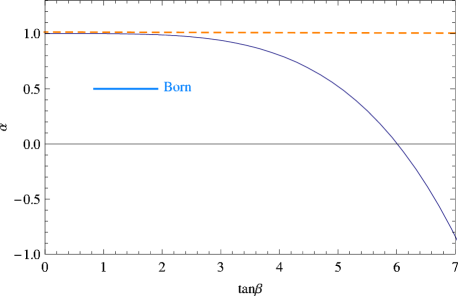
Figure 2: Ratio of polarized decay rates at the Born-level for two models ($\alpha=\Gamma_{0}^{2,pol}/\Gamma_{0}^{1,pol}$) as a function of $\tan\beta$.

It is straightforward to compute the Born term contribution to the partial decay rate of the polarized top quark in the 2HDM. According to the interaction Lagrangians (2) and (3), the coupling of the charged-Higgs boson to the bottom and top quarks can either be expressed as a superposition of scalar and pseudoscaler coupling factors or as a superposition of right- and left-chiral coupling factors GHK . Therefore, the Born term amplitude of the process (1) is given by

$$M_{0}=\bar{u_{b}}(a\boldsymbol{1}+b\gamma_{5})u_{t}=\bar{u_{b}}\{g_{t}\frac{1+\gamma_{5}}{2}+g_{b}\frac{1-\gamma_{5}}{2}\}u_{t},$$ (9)

where, $a$ and $b$ depend on the model and given in (II) and (II). One also has $g_{t}=a+b$ and $g_{b}=a-b$.
For the amplitude squared, one has

$$|M_{0}|^{2} = \sum_{s_{b}}M_{0}^{\dagger}M_{0}=2(p_{b}\cdot p_{t})(a^{2}+b^{2})+$$ (10)

$$2(a^{2}-b^{2})m_{b}m_{t}+4abm_{t}(p_{b}\cdot s_{t}),$$

where we replaced $\sum_{s_{t}}u(p_{t},s_{t})\bar{u}(p_{t},s_{t})=(\displaystyle{\not}{p}_{t}+m_{t})$ in the unpolarized Dirac string by $u(p_{t},s_{t})\bar{u}(p_{t},s_{t})=(1-\gamma_{5}\displaystyle{\not}{s}_{t})(\displaystyle{\not}{p}_{t}+m_{t})/2$ in the polarized state.
Considering Fig. 1, the polarization four-vector of the top quark in the top rest frame reads; $s_{t}=P(0;\sin\theta_{P}\cos\phi_{P},\sin\theta_{P}\sin\phi_{P},\cos\theta_{P})$ so that one has $p_{b}\cdot s_{t}=P(|\vec{p}_{b}|\cos\theta_{P})$. Therefore, the polarized tree-level decay width reads

$$\Gamma_{0}^{pol} = \frac{m_{t}}{8\pi}\lambda(1,\frac{m_{b}^{2}}{m_{t}^{2}},\frac{m_{H^{+}}^{2}}{m_{t}^{2}})(ab),$$ (11)

where $\lambda(x,y,z)=(x-y-z)^{2}-4yz$ is the Källén function. The above result is in complete agreement with Refs. kadeer ; Liud . The unpolarized Born-level rate can be found in our previous work MoosaviNejad:2011yp . In (11) for the product of two coupling factors, in the model $1$, one has

$$ab=\frac{G_{F}}{\sqrt{2}}|V_{tb}|^{2}(m_{t}^{2}-m_{b}^{2})\cot^{2}\beta,$$ (12)

and for the model 2,

$$ab=\frac{G_{F}}{\sqrt{2}}|V_{tb}|^{2}(m_{t}^{2}\cot^{2}\beta-m_{b}^{2}\tan^{2}\beta).$$ (13)

Considering (11) and (13), it is seen that in the model 2 the rate becomes zero when $\tan\beta=\sqrt{m_{t}/m_{b}}\approx 6$ if we take $m_{t}=172.9$ GeV and $m_{b}=4.78$ GeV.
Defining $\alpha=\Gamma_{0}^{2,pol}/\Gamma_{0}^{1,pol}$ as a ratio of polarized Born widths in the models 1 and 2, in Fig. 2 we plot this ratio as a function of $\tan\beta$. Note that, this ratio is independent of the charged Higgs boson mass and for $\tan\beta<4$ (with $\alpha\approx 1$) the Born rates are the same in both models. $\alpha$ is positive/negative for small/large values of $\tan\beta$ and goes through zero for $\tan\beta=6.01$.
In this work, we adopt the massless scheme or Zero-Mass Variable-Flavor-Number (ZM-VFN) scheme jm where the zero mass parton approximation is also applied to the bottom quark. In kadeer , it is shown that the $m_{b}=0$ approximation can be quite good in both models, see Figs. 5a and b of this reference.

In the limit of vanishing b-quark mass, the tree-level decay width is simplified to

$$\Gamma_{0}=\frac{m_{t}}{8\pi}(1-\frac{m_{H^{+}}^{2}}{m_{t}^{2}})^{2}(ab).$$ (14)

In the following, in a detailed discussion we calculate the ${\cal O}(\alpha_{s})$ QCD corrections to the Born-level decay rate of $t\rightarrow bH^{+}$ and we present, for the first time, the analytical parton-level expressions for $d\Gamma(t(\uparrow)\rightarrow BH^{+}+X)/dx_{B}$ at NLO in the ZM-VFN scheme.

II.2 ${\cal O}(\alpha_{s})$ virtual corrections

The ${\cal O}(\alpha_{s})$ one-loop vertex corrections to the $tbH^{+}$-vertex arise from the emission and absorption of the virtual gluons from top and bottom quark legs in Feynman diagrams. Considering the interaction of the quark fields $q(x^{\mu})$ with gluons which includes a vector-like coupling as

$$g_{s}\bar{q}_{i}(x)\gamma^{\mu}T^{a}_{ij}q_{j}(x)G^{a}_{\mu}(x),$$ (15)

one can extract the Feynman rules to calculate the virtual radiative corrections. In (15), $g_{s}$ is the strong coupling constant, $a=1,2,\cdots,8$ is the QCD color index of gluons so for the SU(3) generator $T^{a}$ one has $Tr(T^{a}T^{a})=4$.
In the massless-scheme where $m_{b}=0$ is considered, the virtual one-loop corrections consist of both infrared (IR) and ultraviolet (UV) divergences in which, for example, the UV-divergences appear when the integration region of the internal momentum of the virtual gluon goes to infinity. Here, we adopt the "on-shell" mass renormalization scheme and use dimensional regularization to regulate all singularities. In this scheme, all divergences are regularized in $D=4-2\epsilon$ (with $\epsilon\ll 1$) space-time dimensions to become single poles in $\epsilon$.

Considering the scaled-energy variable (8), which is now simplified in the massless scheme as

$$x_{b}=\frac{2E_{b}}{m_{t}(1-y)},$$ (16)

the contribution of virtual corrections into the doubly differential decay width (7) is given by

$$\frac{d^{2}\Gamma^{\textbf{vir}}_{b}}{dx_{b}d\cos\theta_{P}}=\frac{|M^{\textbf{vir}}|^{2}}{32\pi m_{t}}(1-y)\delta(1-x_{b}),$$ (17)

where, $|M^{\textbf{vir}}|^{2}=\sum_{s_{b}}(M_{0}^{\dagger}M_{loop}+M_{loop}^{\dagger}M_{0})$. The Born amplitude $M_{0}$ is given in (9) and following Refs. Czarnecki ; Liud , the renormalized amplitude of the virtual corrections is written as

$$M_{loop}=\bar{u_{b}}(\Lambda_{ct}+\Lambda_{l})(a+b\gamma_{5})u_{t},$$ (18)

where $\Lambda_{l}$ stands for the one-loop vertex correction and $\Lambda_{ct}$ refers to the counter term of the vertex. The analytical form of the counter term (including the mass and the wave-function renormalizations of the top and bottom quarks), and the one-loop vertex correction $\Lambda_{l}$ can be found in MoosaviNejad:2011yp when the massless-scheme is applied. For the massive scheme (where $m_{b}\neq 0$) these forms can be found in MoosaviNejad:2012ju .
Note that, after summing all virtual corrections up all UV-divergences are canceled but the IR-singularities are remaining which, from now on, we label them by $\epsilon$.
Therefore, the virtual corrections to the differential decay width (7) is presented by

$$\frac{d^{2}\Gamma^{\textbf{vir}}}{dx_{b}d\cos\theta_{P}}=\frac{1}{2}\bigg{\{}\frac{d\Gamma^{\textbf{vir,unpol}}}{dx_{b}}+P\frac{d\Gamma^{\textbf{vir,pol}}}{dx_{b}}\cos\theta_{P}\bigg{\}},$$ (19)

where $d\Gamma^{\textbf{vir,unpol}}/dx_{b}$ is given in MoosaviNejad:2011yp and for the polarized rate, normalized to the polarized Born width (14), one has

$$\frac{1}{\Gamma_{0}}\frac{d\Gamma^{\textbf{vir,pol}}}{dx_{b}} = \frac{\alpha_{s}(\mu_{R})}{2\pi}C_{F}\delta(1-x_{b})\big{(}-\frac{1}{\epsilon^{2}}+\frac{F}{\epsilon}-\frac{F^{2}}{2}+$$

$$(\frac{2}{y}-5)\ln(1-y)-2Li_{2}(y)-\frac{7}{8}-\frac{\pi^{2}}{12}\big{)}.$$

Here, $C_{F}=(N_{c}^{2}-1)/(2N_{c})=4/3$ for $N_{c}=3$ quark colors, $Li_{2}(y)$ is the Spence function and the term $F$ reads

$$F=2\ln(1-y)-\ln\frac{4\pi\mu_{F}^{2}}{m_{t}^{2}}+\gamma_{E}-\frac{5}{2},$$ (21)

where $\mu_{F}$ is the factorization scale and $\gamma_{E}=0.5772\cdots$ is the Euler constant.
The renormalized virtual one-loop correction (II.2) is in complete agreement with kadeer . Although, this comparison is not so straightforward, because in kadeer authors regularized the UV singularities using the D-dimensional regularization scheme (as we have done) but to regulate the IR divergences they introduced a finite (small) gluon mass $m_{g}\neq 0$ in the gluon propagator. Then, to compare the extracted results one has to consider the replacement; $1/\epsilon-\gamma_{E}+\ln(4\pi\mu_{F}^{2}/m_{t}^{2})\to\ln(m_{g}^{2}/m_{t}^{2})$. However, all the logarithmic gluon mass dependence or/and the singular terms in the form of $1/\epsilon$ resulting from the different regularization procedures must be canceled out when the virtual and tree-graph contributions are summed up.

II.3 Tree-graph contributions

Figure 3: Definition of the polar angle $\theta_{P}$ in the helicity coordinate system selected for the NLO QCD corrections. $\vec{P}_{t}$ is the polarization vector of the top quark.

In the rest frame of a top quark decaying into a bottom quark, a Higgs boson and a gluon, the outgoing particles define an event plane. Relative to this plane we can define the spin direction of the polarized top quark. Therefore, for the NLO analysis of the spin-momentum correlation between the top quark polarization vector and the momenta of its decay products we apply the helicity coordinate system shown in Fig. 3. In this system the polarization vector of the top quark is evaluated relative to the Higgs boson 3-momentum which points to the direction of the positive $z$-axis.
The QCD NLO contribution to the differential decay rate results from the square of the amplitudes as $|M_{0}|^{2}$ (10), $|M^{\textbf{vir}}|^{2}$ (18) and $|M^{\textbf{real}}|^{2}=M^{\textbf{real}\dagger}\cdot M^{\textbf{real}}$, where $M^{\textbf{real}}$ stands for the real gluon (tree-graph) contribution, $t(\uparrow)\to bH^{+}+g$, which reads

$$M^{\textbf{real}} = g_{s}\frac{\lambda^{a}}{2}\bar{u}(p_{b},s_{b})\big{\{}\frac{2p_{t}^{\mu}-\displaystyle{\not}p_{g}\gamma^{\mu}}{2p_{t}\cdot p_{g}}$$

$$-\frac{2p_{b}^{\mu}+\gamma^{\mu}\displaystyle{\not}p_{g}}{2p_{b}\cdot p_{g}}\big{\}}(a\textbf{1}+b\gamma_{5})u(p_{t},s_{t})\epsilon_{\mu}^{\star}(p_{g},r),$$

where $\epsilon(p_{g},r)$ stands for the polarization vector of the emitted real gluon with the momentum $p_{g}$ and spin $r$. In (II.3), the first and second terms refer to real gluon emission from the top quark and the bottom quark, respectively. As before, in order to regulate the IR-divergences, which arise from the soft- and collinear-gluon emissions, we work in $D-$dimensions. In this scheme, the differential decay rate for the real emission contribution is given by

$$d\Gamma^{\textbf{real}}=\frac{\mu_{F}^{2(4-D)}}{2m_{t}}|M^{\textbf{real}}|^{2}dR_{3}(p_{t},p_{b},p_{g},p_{{}_{H^{+}}}),$$ (23)

where, the phase space element $dR_{3}$ is

$$\frac{d^{D-1}\mathbb{p}_{b}}{2E_{b}}\frac{d^{D-1}\mathbb{p}_{H}}{2E_{H}}\frac{d^{D-1}\mathbb{p}_{g}}{2E_{g}}(2\pi)^{3-2D}\delta^{D}(p_{t}-\sum_{g,b,H}p_{f}).$$

To evaluate the real doubly differential decay rate normalized to the polarized Born width (14), i.e. $1/\Gamma_{0}\times d^{2}\Gamma^{\textbf{real}}/(dx_{b}d\cos\theta_{P})$, we fix the momentum of b-quark in (23) and integrate over the energy of the $H^{+}$-boson which ranges as

$$m_{t}\frac{y+[1-x_{b}(1-y)]^{2}}{2[1-x_{b}(1-y)]}\leq E_{H}\leq m_{t}\frac{1+y}{2}.$$ (25)

To compute the angular distribution of differential width, the angular integral in (II.3) has to be written as $d^{D-1}\mathbb{p}_{{}_{H}}=\mathbb{p}_{{}_{H}}^{D-2}d\mathbb{p}_{{}_{H}}d\Omega_{H}$ in which

$$d\Omega_{H}=-\frac{2\pi^{\frac{D}{2}-1}}{\Gamma(\frac{D}{2}-1)}(\sin\theta_{P})^{D-4}d\cos\theta_{P}.$$ (26)

Therefore, the polarized doubly differential width reads

$$\frac{d^{2}\Gamma^{\textbf{real,pol}}}{dx_{b}d\cos\theta_{P}} = Ax_{b}^{D-4}|M^{real}|^{2}(1-\cos^{2}\alpha)^{\frac{D-4}{2}}\times$$ (27)

$$\delta(\cos\alpha-b)dE_{H}d\cos\alpha,$$

where the angles $\theta_{P}$ and $\alpha$ are defined in Fig. 3, and

$$A=\mu_{F}^{2(4-D)}(p_{H}m_{t})^{D-4}\frac{(1-y)^{D-3}}{2^{3D-4}\pi^{D-1}\Gamma^{2}(\frac{D}{2}-1)}.$$ (28)

In the equation above, $b=(m_{t}^{2}+m_{H}^{2}-2m_{t}(E_{b}+E_{H})+2E_{b}E_{H})/(2E_{b}p_{H})$ and $p_{H}=\sqrt{E_{H}^{2}-m_{H}^{2}}$ is the 3-momentum of the Higgs boson.
Considering Fig. 3, the relevant scalar products evaluated in the top rest frame are

$$p_{H}\cdot s_{t} = -P(p_{H}\cos\theta_{P}),$$

$$p_{b}\cdot s_{t} = -P(E_{b}\cos\alpha\cos\theta_{P}),$$ (29)

$$p_{b}\cdot p_{H} = E_{b}(E_{H}-p_{H}\cos\alpha),$$

and $p_{t}\cdot s_{t}=0$. Here $P$ refers to the polarization degree of the top quark.

It should be noted that, since the real correction contribution includes the pole $\propto 1/\epsilon$, therefore, to get the correct finite terms in the normalized differential distributions the Born width $\Gamma_{0}$ (14) must be evaluated in the dimensional regularization at ${\cal O}(\epsilon)$, i.e. $\Gamma_{0}\rightarrow\Gamma_{0}\{1-\epsilon\big{[}2\ln(1-y)-2\ln 2+\gamma_{E}-\ln(4\pi\mu_{F}^{2}/m_{t}^{2})\big{]}\}$.

As a last technical point; when one integrates over the phase space for the real gluon radiation, terms of the form $(1-x_{b})^{-1-2\epsilon}$ arise which are due to the radiation of a soft gluon in top decay. In fact, the limit of $E_{g}\to 0$ corresponds to the limit $x_{b}\to 1$. Therefore, we use the following expression Corcella:1

$$(1-x_{b})^{-1-2\epsilon} =-\frac{1}{2\epsilon}\delta(1-x_{b})+\bigg{(}\frac{1}{1-x_{b}}\bigg{)}_{+}$$ (30)

$$-2\epsilon\bigg{(}\frac{\ln(1-x_{b})}{1-x_{b}}\bigg{)}_{+},$$

where the plus distribution is defined as

$$\int_{0}^{1}(f(x_{b}))_{{}_{+}}h(x_{b})dx_{b}=\int_{0}^{1}f(x_{b})[h(x_{b})-h(1)]dx_{b}.$$ (31)

II.4 Analytical results for differential decay rates $d\Gamma/dx_{i}$ at parton level

According to Eq. (7), the ${\cal O}(\alpha_{s})$ correction to the angular distribution of partial decay rates is obtained by summing the Born, the virtual and the real gluon contributions and is given by

$$\frac{d^{2}\Gamma_{\textbf{nlo}}}{dx_{b}d\cos\theta_{P}}=\frac{1}{2}\bigg{\{}\frac{d\Gamma^{\textbf{unpol}}_{\textbf{nlo}}}{dx_{b}}+P\frac{d\Gamma^{\textbf{pol}}_{\textbf{nlo}}}{dx_{b}}\cos\theta_{P}\bigg{\}}.$$ (32)

The unpolarized rate $d\Gamma^{\textbf{unpol}}/dx_{b}$ is given in MoosaviNejad:2011yp and for the polarized one, normalized to the Born rate (14), one has

$$\frac{1}{\Gamma_{0}}\frac{d\Gamma^{\textbf{pol}}_{\textbf{nlo}}}{dx_{b}} = \delta(1-x_{b})+\frac{C_{F}\alpha_{s}}{2\pi}\Big{\{}[-\frac{1}{\epsilon}+\gamma_{E}-\ln 4\pi]$$ (33)

$$\times[\frac{3}{2}\delta(1-x_{b})+\frac{1+x_{b}^{2}}{(1-x_{b})_{+}}]+T_{1}\Big{\}},$$

where, by defining $S=(1-y)/2$ (with $y=m_{H}^{2}/m_{t}^{2}$) one has

$$T_{1} = \delta(1-x_{b})\bigg{\{}-\frac{3}{2}\ln\frac{\mu_{F}^{2}}{m_{t}^{2}}+\frac{4S}{y}\ln(1-y)-\frac{7\pi^{2}}{3}$$

$$+2Li_{2}(1-y)-2Li_{2}(y)-\frac{y}{S}\ln(y)-4\bigg{\}}$$

$$+2(1+x_{b}^{2})\bigg{(}\frac{\ln(1-x_{b})}{1-x_{b}}\bigg{)}_{+}$$

$$+2\frac{1+x_{b}^{2}}{(1-x_{b})_{+}}\ln\frac{m_{t}x_{b}(1-y)}{\mu_{F}}+1-x_{b}-R_{2}\frac{1+x_{b}^{2}}{1-x_{b}}$$

$$-\frac{y}{S(1-x_{b})}+\frac{1-S}{S(Sx_{b}^{2}-2x_{b}+2)}+$$

$$\frac{|2Sx_{b}^{2}-2x_{b}+1|}{Sx_{b}^{2}-2x_{b}+2}\bigg{(}\frac{1}{1-x_{b}}+\frac{1-Sx_{b}}{S}\bigg{)}+$$

$$R_{1}\sqrt{\frac{Sx_{b}^{2}-2x_{b}+2}{S}}\bigg{(}\frac{1+x_{b}}{1-x_{b}}+\frac{x_{b}S^{2}-Sx_{b}-1}{S(Sx_{b}^{2}-2x_{b}+2)}+$$

$$\frac{1-S-x_{b}(1-S)^{2}}{S(Sx_{b}^{2}-2x_{b}+2)^{2}}\bigg{)}.$$

Here, we also defined

$$R_{1} = \ln\bigg{(}1-2S^{2}x_{b}^{3}+4Sx_{b}^{2}-3Sx_{b}-x_{b}+$$ (35)

$$\sqrt{S(Sx_{b}^{2}-2x_{b}+2)}|2Sx_{b}^{2}-2x_{b}+1|\bigg{)},$$

$$R_{2} = \ln\bigg{(}(1-S)x_{b}^{2}-x_{b}+\frac{1}{2}+\frac{|2Sx_{b}^{2}-2x_{b}+1|}{2}\bigg{)}.$$

This differential decay rate (33) after integration over $x_{b}$ ($0\leq x_{b}\leq 1$) is in complete agreement with the result presented in kadeer .

Since, observable hadrons through top decays can be also produced from the fragmentation of the emitted real gluons, therefore, to obtain the most accurate energy spectrum of produced hadrons one has to add the contribution of gluon fragmentation to the b-quark one to produce the outgoing hadron. As shown in Nejad:2013fba , the gluon splitting contribution is important at a low energy of the observed hadron so this decreases the size of decay rate at the threshold. Then, we also need the polarized differential decay rate $d\Gamma^{\textbf{pol}}_{\textbf{nlo}}/dx_{g}$, where $x_{g}=2E_{g}/(m_{t}(1-y))$ is the scaled-energy fraction of the real gluon, as in (16). Considering the general form of the angular distribution (32), the unpolarized rate $d\Gamma^{\textbf{unpol}}/dx_{g}$ is given in MoosaviNejad:2011yp and for the polarized one we proceed as follows. In (23), we fix the momentum of gluon in the three-body phase space and integrate over the energy of the $H^{+}$-boson which ranges as

$$m_{t}\frac{y+[1-x_{g}(1-y)]^{2}}{2[1-x_{g}(1-y)]}\leq E_{H}\leq m_{t}\frac{1+y}{2}.$$ (36)

Therefore, the polarized doubly differential decay rate is obtained by

$$\frac{d^{2}\Gamma^{\textbf{pol}}}{dx_{g}d\cos\theta_{P}} \propto x_{g}^{D-4}|M^{real}|^{2}(1-\cos^{2}\theta)^{\frac{D-4}{2}}\times$$ (37)

$$\delta(\cos\theta-a)dE_{H}d\cos\theta,$$

where, the proportionality coefficient is the same as in (28) and $\theta$ is the angle between the 3-momentum of the gluon and the Higgs boson (see Fig. 3), whereas $a=(m_{t}^{2}+m_{H}^{2}-2m_{t}(E_{g}+E_{H})+2E_{g}E_{H})/(2E_{g}p_{H})$. The required four-momentum scalar products are

$$p_{H}\cdot s_{t} = -P(p_{H}\cos\theta_{P}),$$

$$p_{g}\cdot s_{t} = -P(E_{g}\cos\theta\cos\theta_{P}),$$ (38)

$$p_{g}\cdot p_{H} = E_{g}(E_{H}-p_{H}\cos\theta).$$

Therefore the polarized differential width, normalized to the Born rate (14), is expressed as

$$\frac{1}{\Gamma_{0}}\frac{d\Gamma^{\textbf{pol}}_{\textbf{nlo}}}{dx_{g}} = \frac{C_{F}\alpha_{s}}{2\pi}\bigg{\{}\frac{1+(1-x_{g})^{2}}{x_{g}}(-\frac{1}{\epsilon}+\gamma_{E}-\ln 4\pi)$$ (39)

$$+T_{2}\bigg{\}},$$

where,

$$T_{2} = \frac{1+(1-x_{g})^{2}}{x_{g}}\bigg{(}-B_{2}+2\ln\frac{2Sx_{g}(1-x_{g})m_{t}}{\mu_{F}}\bigg{)}$$ (40)

$$+\frac{1-S(1+3x_{g})+x_{g}S^{2}(2x_{g}^{2}+4x_{g}-3)}{2S^{2}x_{g}^{2}}+$$

$$\frac{B_{1}}{2S^{3}x_{g}^{2}}\bigg{(}1-S(3x_{g}+2)-2x_{g}S^{3}(x_{g}^{2}-2x_{g}+2)$$

$$+2S^{2}(1+x_{g})^{2}\bigg{)}+\frac{|2Sx_{g}^{2}-2x_{g}+1|}{2S^{2}x_{g}^{2}(1-2Sx_{g})^{2}}\bigg{(}6S^{3}x_{g}^{3}$$

$$-4S^{3}x_{g}^{2}-x_{g}(1+8x_{g})S^{2}+5Sx_{g}+S-1\bigg{)},$$

and

$$B_{1} = \ln\bigg{(}2S^{2}x_{g}^{2}-2Sx_{g}-S+1+S|2Sx_{g}^{2}-2x_{g}+1|\bigg{)}$$ (41)

$$-\ln(1-2Sx_{g}),$$

$$B_{2} = \ln\bigg{(}(1-S)x_{g}^{2}-x_{g}+\frac{1}{2}+\frac{|2Sx_{g}^{2}-2x_{g}+1|}{2}\bigg{)}.$$

In Eqs. (33) and (39), $T_{1}$ and $T_{2}$ are free of all divergences and to subtract the singularities remaining in the polarized differential decay widths, we apply the modified minimal-subtraction $(\overline{MS})$ scheme where, the singularities are absorbed into the bare fragmentation functions. This renormalizes the fragmentation functions and creates the finite terms of the form $\alpha_{s}\ln(m_{t}^{2}/\mu_{F}^{2})$ in the polarized differential widths. Following this scheme, to obtain the $\overline{MS}$ coefficient functions one has to subtract from (33) and (39), the ${\cal O}(\alpha_{s})$ term multiplying the characteristic $\overline{MS}$ constant $(-1/\epsilon+\gamma_{E}-\ln 4\pi)$Corcella:1 .
In this work we set $\mu_{F}=m_{t}$, so that in Eqs. (II.4) and (40) the terms proportional to $\alpha_{s}\ln(m_{t}^{2}/\mu_{F}^{2})$ vanish.

III Numerical results

Having the parton-level differential decay widths (33) and (39), we are now in a situation to present our phenomenological predictions for the scaled-energy ($x_{B}$) distribution of bottom-flavored hadrons (B) inclusively produced in polarized top decay in the 2HDM. To indicate our predictions for the $x_{B}$-distribution, we consider the doubly differential distribution $d^{2}\Gamma/(dx_{B}d\cos\theta_{P})$ of the partial width of the decay $t(\uparrow)\rightarrow BH^{+}+X$. Here, as in (16), $x_{B}=2E_{B}/(m_{t}(1-y))$ is the scaled-energy fraction of the B-hadron in the top quark rest frame, where the B-hadron energy ranges from $E_{B}^{min}=m_{B}$ to $E_{B}^{max}=(m_{t}^{2}+m_{B}^{2}-m_{H}^{2})/(2m_{t})$.

In general case, according to the factorization theorem of QCD-improved parton model collins , the B-hadron energy distribution can be expressed as the convolution of the parton-level spectrum $d\Gamma/dx_{a}(a=b,g)$ with the nonperturbative fragmentation function $D_{a}^{B}(z,\mu_{F})$ which describes the hadronization process $a\to B$ at the scale $\mu_{F}$, i.e.

$$\frac{d\Gamma}{dx_{B}}=\sum_{a=b,g}\int_{x_{a}^{\text{min}}}^{x_{a}^{\text{max}}}\frac{dx_{a}}{x_{a}}\,\frac{d\Gamma}{dx_{a}}(\mu_{R},\mu_{F})D_{a}^{B}(\frac{x_{B}}{x_{a}},\mu_{F}),$$ (42)

where, $\mu_{R}$ is the renormalization scale related to the renormalization of the QCD coupling constant and $\mu_{F}$ is the factorization scale. We shall use the convention $\mu_{R}=\mu_{F}=m_{t}$ for our results, a choice often made.

In the MSSM, the mass of $H^{\pm}$ is strongly correlated with the mass of other Higgs bosons. In this model, the charged Higgs boson mass is restricted at tree-level by $m_{H^{+}}>m_{W}$ Nakamura:2010zzi , but this restriction does not hold for some regions of parameter space after including radiative corrections. In Ali:2009sm , it is mentioned that a $H^{\pm}$ boson with a mass in the range $80GeV\leq m_{H^{\pm}}\leq 160GeV$ is a logical possibility and its effects should be searched for in the decays $t\rightarrow bH^{+}\rightarrow B\tau^{+}\nu_{\tau}+X$.
On the other hand, the recent results of a search for evidence of a charged Higgs boson in $19.5-19.7fb^{-1}$ of proton-proton collision data recorded at $\sqrt{s}=8$ TeV are reported by the CMS CMS:2014cdp and the ATLAS TheATLAScollaboration:2013wia experiments at the CERN LHC. Their results show that the large region in the MSSM $m_{H^{+}}-\tan\beta$ parameter space for $m_{H^{+}}=80-160$ GeV is excluded and only some regions of the parameter space are still unexcluded. These regions along with the $\pm 1\sigma$ band around the expected limit are shown in Fig. 4 which is taken from Ref. TheATLAScollaboration:2013wia . A same exclusion is reported by the CMS CMS:2014cdp collaboration. However, a definitive search of the charged-Higgses over this part of the $m_{H^{+}}-\tan\beta$ plane in the MSSM is a program that still has to be carried out and this belongs to the LHC experiments.

For our numerical analysis, from Ref. Nakamura:2010zzi we adopt the input parameter values $G_{F}=1.16637\times 10^{-5}$ GeV^-2, $m_{t}=172.98$ GeV, $m_{W}=80.399$ GeV, $m_{B}=5.279$ GeV, and $|V_{tb}|=0.999152$. We evaluate the QCD coupling constant $\alpha_{s}^{(n_{f})}(\mu_{R})$ at NLO in the $\overline{\text{MS}}$ scheme using

$$\alpha^{(n_{f})}_{s}(\mu)=\frac{1}{b_{0}\log(\mu^{2}/\Lambda^{2})}\Big{\{}1-\frac{b_{1}\log\big{[}\log(\mu^{2}/\Lambda^{2})\big{]}}{b_{0}^{2}\log(\mu^{2}/\Lambda^{2})}\Big{\}},$$

where $n_{f}$ is the number of active quark flavors, and $b_{0}$ and $b_{1}$ are given by

$$b_{0}=\frac{33-2n_{f}}{12\pi},\quad b_{1}=\frac{153-19n_{f}}{24\pi^{2}},$$ (44)

where $\Lambda$ is the typical QCD scale. Here, we adopt $\Lambda_{\overline{\text{MS}}}^{(5)}=231.0$ MeV adjusted such that $\alpha_{s}^{(5)}=0.1184$ for $m_{Z}=91.1876$ GeV Nakamura:2010zzi . To describe the splitting $(b,g)\rightarrow B$, we employ the realistic nonperturbative $B$-hadron fragmentation functions determined at NLO in the ZM-VFN scheme through a global fit to electron-positron annihilation data presented by ALEPH Heister:2001jg and OPAL Abbiendi:2002vt at CERN LEP1 and by SLD Abe:1999ki at SLAC SLC. Specifically, for the $b\to B$ splitting a simple power model as; $D_{b}(z,\mu_{F}^{\text{ini}})=Nz^{\alpha}(1-z)^{\beta}$ was used at the initial scale $\mu_{F}^{\text{ini}}=4.5$ GeV, while the gluon and light-quark fragmentation functions were generated via the DGLAP evolution equations dglap . The fit results the values $N=4684.1$, $\alpha=16.87$, and $\beta=2.628$ Kniehl:2008zza for the fragmentation function parameters.

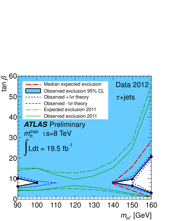
Figure 4: Exclusion region in the MSSM $\tan\beta-m_{H^{+}}$ parameter space for $m_{H^{+}}=80-160$ GeV is shown. The $\pm 1\sigma$ band around the expected limit is also shown. The blue region is excluded. Plot is got from Ref. TheATLAScollaboration:2013wia .

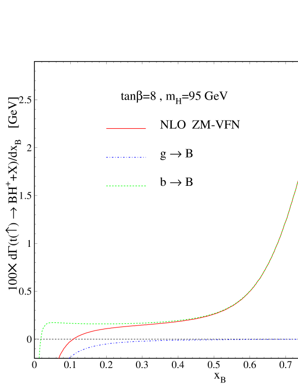
Figure 5: $d\Gamma/dx_{B}$ as a function of $x_{B}$ in the 2HDM with $m_{H^{+}}=95$ GeV and $\tan\beta=8$. The NLO result (solid line) is broken up into the contributions due to $b\to B$ (dashed line) and $g\to B$ (dot-dashed line) fragmentation.

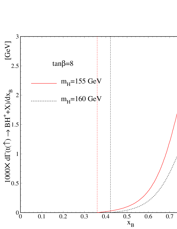
Figure 6: $x_{B}$ spectrum in polarized top decay in the 2HDM with $\tan\beta=8$ and $m_{H^{+}}=155$ and $160$ GeV. Thresholds at $x_{B}$ are also shown. Detail are discussed in the text.

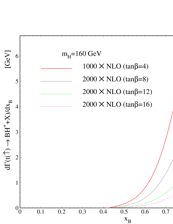
Figure 7: $x_{B}$ spectrum in polarized top decay in the 2HDM $(t(\uparrow)\to BH^{+}+X)$ with different values of $\tan\beta=4$, $8$, $12$ and $16$. The charged Higgs boson mass is fixed to $m_{H^{+}}=160$ GeV. For the large values of $\tan\beta$ the decay rate becomes small.

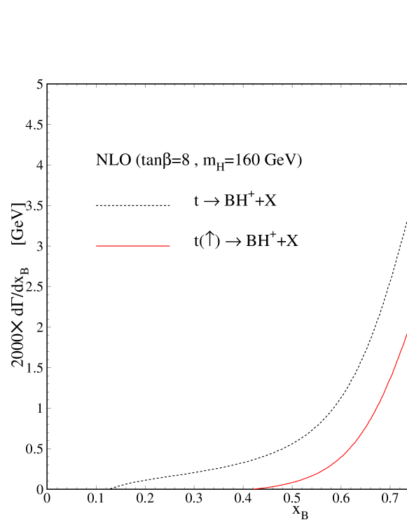
Figure 8: $d\Gamma/dx_{B}$ as a function of $x_{B}$ in the 2HDM considering the ZM-VFN ($m_{b}=0$) scheme. The polarized (solid line) and unpolarized (dashed line) partial decay rates are compared at NLO. We fixed $m_{H^{+}}=160$ GeV and $\tan\beta=8$. We also set $\mu_{R}=\mu_{F}=m_{t}$.

Considering Fig. 4, where the charged Higgs masses $90\leq m_{H^{+}}\leq 100$ GeV (with $6<\tan\beta<10$) and $140\leq m_{H^{+}}\leq 160$ GeV (with $3<\tan\beta<21$) are still unexcluded and could be possible masses, here, we study the scaled-energy spectrum of the B-hadron produced in the polarized top decay in the 2HDM. For this study we consider the distribution $d\Gamma(t(\uparrow)\to BH^{+}+X)/dx_{B}$ in the ZM-VFN scheme.

In Fig. 5, we show our prediction for the size of $d\Gamma/dx_{B}$, by considering the NLO result (solid line) and the relative importance of the $b\to B$ (dashed line) and $g\to B$ (dot-dashed line) fragmentation channels at NLO, taking $\tan\beta=8$ and $m_{H^{+}}=95$ GeV. As is seen, the gluon fragmentation leads to an appreciable reduction in decay rate at low-$x_{B}$ region, for $x_{B}<0.35$. For example, the gluon splitting decreases the size of decay rate up to $45\%$ at $x_{B}=0.14$. For higher values of $x_{B}$, the $b\to B$ contribution is absolutely dominant.

In Fig. 6, we show our prediction for the size of the NLO corrections for $m_{H^{+}}=155$ (solid line) and $m_{H^{+}}=160$ GeV (dashed line) where $\tan\beta$ is set to $\tan\beta=8$. Here, the B-hadron mass creates a threshold, e.g. at $x_{B}=2m_{B}/(m_{t}(1-y))\approx 0.42$ for $m_{H^{+}}=160$ GeV. As is seen, when $m_{H^{+}}$ increases the size of decay rate decreases but the peak position is approximately constant and independent of the charged Higgs mass.

Considering the unexcluded region from Fig. 4 where $3\leq\tan\beta\leq 21$ is allowed for $m_{H^{+}}=160$ GeV, in Fig. 7 we study the energy spectrum of the B-hadron for different values of the $\tan\beta=4$, $8$, $12$ and $16$, where the mass of Higgs boson is fixed to $m_{H^{+}}=160$ GeV. As is seen when $\tan\beta$ increases the decay rate decreases, as $\Gamma_{0}$ (14) is proportional to $\cot^{2}\beta$.

In Fig. 8, the NLO energy spectrum of B-hadrons from the unpolarized top decays $t\rightarrow BH^{+}+X$ (dashed line) and the polarized ones $t(\uparrow)\rightarrow BH^{+}+X$ (solid line) are compared considering $\tan\beta=8$ and $m_{H^{+}}=160$ GeV. Our results show that in these two cases the NLO corrections are similar in shape, however, the unpolarized distribution shows an more enhancement in size at NLO.

Our formalism elaborated here can be also extended to the production of hadron species other than bottom-flavored hadrons, such as pions, kaons and protons, etc., using the nonperturbative $(b,g)\rightarrow\pi/K/P$ FFs extracted in our recent works Soleymaninia:2013cxa ; Nejad:2015fdh , relying on their universality and scaling violations.

IV Conclusions

The top quark is the heaviest elementary particle so that its large mass is a reason to rapid decay and, therefore, it has no time to hadronize. Thus, it remains its full polarization content when it decays. Due to $|V_{tb}|\approx 1$ of the CKM matrix, top quark decays are completely dominated by the mode $t\rightarrow W^{+}+b$ within the SM to a very high accuracy and in the theories beyond the SM including the two-Higgs-doublet, the decay mode of light charged Higgses ($m_{H^{\pm}}<m_{t}$) is occurred via $t\rightarrow H^{+}+b$. The charged-Higgs bosons have been searched for in high energy experiments, in particular, at LEP and the Tevatron but they have not been seen so far. But further searches are in progress so their discovery would indicate a signal of new physics beyond the SM. Among other things, the CERN LHC is a great top factory, producing around 90 million top pairs per year of running at design c.m. energy of 14 TeV. The existing and updating data will allow us to search for the charged Higgs boson if also the theoretical description and simulations are of proportionate quality.

Since, bottom quarks produced through top decays hadronize before they decay, then each $b$-jet includes a bottom flavored hadron which, most of the times, is a B-meson. These mesons are identified by a displaced decay vertex associated which charged lepton tracks.
At LHC, the decay process $t\rightarrow BH^{+}+X$ is proposed to search for the light charged Higgs bosons and evaluating the distribution in the scaled-energy ($x_{B}$) of B-mesons in the top quark rest frame would be of particular interest. For this study, one needs to evaluate the quantity $d\Gamma/dx_{B}$. The comparison of future measurements of $d\Gamma/dx_{B}$ at the LHC with our NLO predictions will be important for future tests of the Higgs coupling in the minimal supersymmetric SM (MSSM).
In the present work, using the ZM-VFN scheme we studied the $x_{B}$-distribution of B-meson in the decay mode $t(\uparrow)\rightarrow BH^{+}+X$ at NLO by working on the type-I 2HDM scenario or a supersymmetric version of type-II; MSSM.
In order to make our predictions we, first, calculated an analytic expression for the NLO radiative corrections to the differential decay width $d\Gamma(t(\uparrow)\to bH^{+}(+g))/dx_{a}(a=b,g)$ and then employed the nonperturbative $(b,g)\to B$ FFs, relying on their universality and scaling violations collins . For our numerical analysis, considering the recent results reported by the CMS CMS:2014cdp and ATLAS TheATLAScollaboration:2013wia collaborations we restricted ourselves to the unexcluded regions of the $m_{H^{+}}-\tan\beta$ parameter space which include $90\leq m_{H^{+}}\leq 100$ GeV (with $6<\tan\beta<10$) and $140\leq m_{H^{+}}\leq 160$ GeV (with $3<\tan\beta<21$), see Fig. 4.

The top quark polarization is studied by the angular correlations between the top quark spin and its decay products momenta, so these spin-momenta correlations will allow the detailed studies of the top decay mechanism in the 2HDM. In our previous work MoosaviNejad:2011yp , we studied the energy spectrum of B-meson in the 2HDM for the unpolarized decay mode. Here, we also compared the energy spectrum of B-mesons produced both through the unpolarized and polarized top decays. Results show a considerable difference between two distributions, however, they depend on the charged Higgs mass and $\tan\beta$.
Our formalism can be also applied for the production of other hadrons such as pions, kaons and protons, etc., using the nonperturbative $(b,g)\rightarrow\pi/K/P$ FFs presented in Soleymaninia:2013cxa ; Nejad:2015fdh .

V Acknowledgments

We would like to thank Rebeca Gonzalez Suarez from the LHC top working group for reading the manuscript and also for importance discussion and comments. We warmly acknowledge M. Hashemi for valuable discussions and critical remarks. We would also like to thank the CERN TH-PH division for its hospitality where a portion of this work was performed.

References

- (1) G. Aad et al. [ATLAS Collaboration], Phys. Lett. B 716 (2012) 1.
- (2) S. Chatrchyan et al. [CMS Collaboration], Phys. Lett. B 716 (2012) 30.
- (3) T. D. Lee, Phys. Rev. D 8 (1973) 1226.
- (4) A. Djouadi, Phys. Rept. 459, 1 (2008).
- (5) J. F. Gunion and H. E. Haber, Nucl. Phys. B 272, 1 (1986); 402, 567 (1993).
- (6) U. Langenfeld, S. Moch and P. Uwer, arXiv:0907.2527 [hep-ph].
- (7) M. Aoki, R. Guedes, S. Kanemura, S. Moretti, R. Santos and K. Yagyu, Phys. Rev. D 84 (2011) 055028.
- (8) A. Heister et al. [ALEPH Collaboration], Phys. Lett. B 543 (2002) 1.
- (9) J. Abdallah et al. [DELPHI Collaboration], Eur. Phys. J. C 34 (2004) 399.
- (10) P. Achard et al. [L3 Collaboration], Phys. Lett. B 575 (2003) 208.
- (11) G. Abbiendi et al. [OPAL Collaboration], Eur. Phys. J. C 72 (2012) 2076.
- (12) V. Khachatryan et al. [CMS Collaboration], JHEP 1511 (2015) 018.
- (13) CMS Collaboration [CMS Collaboration], CMS-PAS-HIG-14-020.
- (14) The ATLAS collaboration [ATLAS Collaboration], ATLAS-CONF-2013-090.
- (15) A. Kadeer, J. G. Körner, and M. C. Mauser, Eur. Phys. J. C 54, 175 (2008).
- (16) A. Ali, E. A. Kuraev and Y. M. Bystritskiy, Eur. Phys. J. C 67, 377 (2010).
- (17) A. Czarnecki and S. Davidson, Phys. Rev. D 47, 3063 (1993).
- (18) J. Liu and Y. P. Yao, Phys. Rev. D 46, 5196 (1992).
- (19) C. S. Li and T. C. Yuan, Phys. Rev. D 42 (1990) 3088 Erratum: [Phys. Rev. D 47 (1993) 2156].
- (20) S. M. Moosavi Nejad, Phys. Rev. D 85 (2012) 054010.
- (21) G. Mahlon and S. J. Parke, Phys. Rev. D 55 (1997) 7249.
- (22) D. Espriu and J. Manzano, Phys. Rev. D 66 (2002) 114009.
- (23) J. F. Gunion, H. Haber, G. Kane, and S. Dawson, The Higgs Hunter’s Guide (Addison-Wesley, Reading, MAA, 1990), and references therein.
- (24) P. Fayet, Nucl. Phys. B 90 (1975) 104.
- (25) P. Fayet, Phys. Lett. B 64 (1976) 159.
- (26) P. Fayet, Phys. Lett. B 69 (1977) 489.
- (27) S. Dimopoulos and H. Georgi, Nucl. Phys. B 193 (1981) 150.
- (28) M. Misiak et al., Phys. Rev. Lett. 114 (2015) no.22, 221801.
- (29) B. A. Kniehl, G. Kramer and S. M. Moosavi Nejad, Nucl. Phys. B 862 (2012) 720.
-
(30)
J. Binnewies, B.A. Kniehl, and G. Kramer,
Phys. Rev. D 58, 034016 (1998);
M. Cacciari and M. Greco, Nucl. Phys. B421, 530(1994). - (31) S. M. Moosavi Nejad, Eur. Phys. J. C 72 (2012) 2224.
- (32) G. Corcella and A. D. Mitov, Nucl. Phys. B 623, 247 (2002).
- (33) S. M. Moosavi Nejad, Phys. Rev. D 88 (2013) no.9, 094011.
- (34) J. C. Collins, Phys. Rev. D 58, 094002 (1998).
- (35) K. Nakamura et al. (Particle Data Group), J. Phys. G 37, 075021 (2010).
- (36) A. Heister et al. (ALEPH Collaboration), Phys. Lett. B 512, 30 (2001).
- (37) G. Abbiendi et al. (OPAL Collaboration), Eur. Phys. J. C 29, 463 (2003).
- (38) K. Abe et al. (SLD Collaboration), Phys. Rev. Lett. 84, 4300 (2000); Phys. Rev. D 65, 092006 (2002); 66, 079905 (2002).
- (39) V. N. Gribov and L. N. Lipatov, Sov. J. Nucl. Phys. 15, 438 (1972) [Yad. Fiz. 15, 781 (1972)]; G. Altarelli and G. Parisi, Nucl. Phys. B126, 298 (1977); Yu. L. Dokshitzer, Sov. Phys. JETP 46, 641 (1977) [Zh. Eksp. Teor. Fiz. 73, 1216 (1977)].
- (40) B. A. Kniehl, G. Kramer, I. Schienbein, and H. Spiesberger, Phys. Rev. D 77, 014011 (2008).
- (41) M. Soleymaninia, A. N. Khorramian, S. M. Moosavi Nejad and F. Arbabifar, Phys. Rev. D 88 (2013) no.5, 054019.
- (42) S. M. Moosavi Nejad, M. Soleymaninia and A. Maktoubian, Eur. Phys. J. A 52 (2016) no.10, 316.