A selection rule for transitions in PT-symmetric quantum theory

Abstract

Carl Bender and collaborators have developed a quantum theory governed by Hamiltonians that are PT-symmetric rather than Hermitian. To implement this theory, the inner product was redefined to guarantee positive norms of eigenstates of the Hamiltonian. In the general case, which includes arbitrary time-dependence in the Hamiltonian, a modification of the Schrödinger equation is necessary as shown by Gong and Wang to conserve probability. In this paper, we derive the following selection rule: transitions induced by time dependence in a PT-symmetric Hamiltonian cannot occur between normalized states of differing PT-norm. We show three examples of this selection rule in action: two matrix models and one in the continuum.

1 Introduction

In 2002, Carl Bender, Dorje C. Brody and Hugh F. Jones discovered that the Hamiltonian in quantum theory need not be Hermitian [1], provided that it be PT-symmetric. Here, P is parity and T is time reversal. In such a theory, the inner product is redefined such as to produce an always positive norm for any eigenstate of the Hamiltonian. This type of quantum theory is understood and has been studied extensively by Bender and collaborators as well as many other authors [2]. PT-symmetric quantum theory is now a well-established part of physics.

A standard and important calculation in quantum mechanics is to add a time dependent interaction to a time- independent Hamiltonian and calculate the probability of transitions between the energy states of the initial Hamiltonian whose eigenstates are presumed to be completely known. For example, consider a hydrogen atom which at some time encounters an electromagnetic wave. Should the atom be in its ground state, one may compute (in some order of perturbation theory) the probability that at some time in the future the atom will absorb energy from the field and make a transition to a higher energy state (resonant absorption). If the atom is in an excited state, one is interested in calculating the probability that the atom is de-excited and thereby emits a corresponding electromagnetic wave (stimulated emission). In this case, there results a selection rule that the angular momentum change of the atom must be $\Delta\ell=\pm 1$ in order to globally conserve angular momentum. Additional important examples of transitions come to mind, such as a spin flip in systems during magnetic or electron-spin resonance.

In this paper, we will address the corresponding calculations of transition probabilities in non-relativistic PT-symmetric quantum theory. We will derive a general theorem, a selection rule, valid for a PT-symmetric Hamiltonian with arbitrary time-dependence. The paper is organized as follows. Section II presents basic properties of both time independent and time dependent PT symmetric quantum theory and gives the notation to be used in the rest of the paper. In Section III we derive our main result, and in Section IV we give three examples: a matrix model having no transitions and one which does, both illustrating the derived selection rule; then an example of a continuum model for which exact calculations may be made. We end with suggestions and questions for further work.

2 PT-symmetric quantum theory

The Hamiltonian must be PT-symmetric that is,

$$[H,{\cal P\cal T}]=0,$$ (1)

and in the unbroken phase: that is, all of the energy eigenstates of $H$ must also be eigenstates of $\cal P\cal T$. It then follows that all the eigenvalues of $H$ are real. As we illustrate in a later section, the unbroken phase condition may restrict the allowed range of parameters defining the Hamiltonian. Here, the operator $\cal P$ is the standard parity operator: under parity, $p\to-p$, $x\to-x$. $\cal T$ is time reversal: under time reversal, $p\to-p$ and $i\to-i$. The latter requirement of complex conjugation is necessary to preserve the fundamental position-momentum commutation relation $[x,p]=i$ under the combined operation $\cal P\cal T$ (we set $\hbar=1$).

Evolution using the Schrödinger equation with a non-Hermitian Hamiltonian generally does not preserve the usual $L^{2}$ norm $<\psi|\psi>$. Thus PT-symmetric quantum mechanics requires the introduction of a new norm. The PT-symmetric Schrödinger equation does preserve the PT norm $<\psi|\cal P|\psi>$. However, the PT norm is not positive definite. The solution is to introduce the operator $\cal C$ which is defined as follows: the eigenstates of $\cal C$ are the same as those of the Hamiltonian, but the eigenvalues are $\pm 1$ where the plus sign is used if the state has positive PT norm and the negative sign is used if the state has negative PT norm. The (positive definite) norm used in PT-symmetric quantum mechanics is then

$$\langle\psi|W|\psi\rangle=\langle\psi|\cal P\cal C|\psi\rangle.$$ (2)

It follows from the definition of the $\cal C$ operator that it has the following properties:

$$[H,{\cal C}]=0$$ (3)

$$[{\cal P\cal T,C}]=0$$ (4)

$${{\cal C}^{2}}=1$$ (5)

These properties are often used to produce a perturbative series expression for $\cal C$. [3, 4]

So far, we have spoken only about Hamiltonians which are independent of time. In order to obtain information about transitions, we must take into account any time-dependence of the system. In this case (in order to preserve the norm under evolution) the usual Schrödinger equation must be modified to the Gong-Wong (GW) equation, [5]

$$i{\partial\psi\over\partial t}=H(t)\psi-{i\over 2}W^{-1}\dot{W}\psi.$$ (6)

The additional term $\Lambda={i\over 2}W^{-1}\dot{W}$ (the overdot denotes derivative in time) must be subtracted from the Hamiltonian so that if $H$ is time-dependent, all norms as defined with the $W$ operator, Eq.(3), be independent of time. Note that whenever $H$ is independent of time the ${\cal C}$ operator will also be. Hence, will $W$ be also independent of $t$, when the GW equation reduces to the original one of Schrödinger. The presence of $\Lambda(t)$ in the GW equation is a complicating presence, yet essential for the understanding of transitions in PT-symmetric quantum theory which we take up in the next section. Examples of the use of the GW equation will be presented in section IV.

3 Selection rule for time-dependent transitions

In this section, we will state and prove our main result. We assume that our Hamiltonian is time-dependent in an arbitrary way, except that for all time the system remains in the unbroken PT-phase: all of the eigenvalues of $H(t)$, $E_{n}(t)$, are real for all time $t$. While still not generally proved, evidence is strong that the eigenstates of a PT-symmetric Hamiltonian in the unbroken phase form a complete set of states. [6]

Theorem: If a time-dependent PT-symmetric Hamiltonian remains in the unbroken phase, transitions between normalized energy eigenstates of $H$ may be made only between states of the same PT-norm.

In the following, the PT-norms of states will be labeled as $e_{n}$:

$$e_{n}=\langle\psi_{n}|{\cal P}|\psi_{n}\rangle=\pm 1.$$ (7)

We start by deriving some preliminary facts. First, since ${\cal C}^{2}=1$ we have that $0={C}\dot{\cal C}+\dot{\cal C}{\cal C}$ or

$${\cal C}\dot{\cal C}=-\dot{\cal C}{\cal C}.$$ (8)

Second, let $|\psi_{n}\rangle$ be a state of $H(t)$ (itself dependent on $t$). Then, $e_{m}|\psi_{m}\rangle={\cal C}|\psi_{m}\rangle$. Differentiating this equation gives,

$$\dot{\cal C}|\psi_{m}\rangle=(e_{m}-{\cal C})|\dot{\psi}_{m}\rangle.$$ (9)

Next, we note that the $\Lambda$ operator defined above can be written as

$$\Lambda={i\over 2}W^{-1}\dot{W}={i\over 2}({\cal P}{\cal C})^{-1}{\cal P}\dot{\cal C}$$ (10)

$$=-{i\over 2}{\cal C}^{-1}{\cal P}^{-1}{\cal P}\dot{\cal C}={i\over 2}{\cal C}\dot{\cal C}$$ (11)

$$=-{i\over 2}\dot{\cal C}{\cal C}.$$ (12)

Thus, the GW equation is,

$$H|\Psi(t)\rangle+{i\over 2}\dot{\cal C}{\cal C}|\Psi(t)\rangle=i{\partial\Psi\over\partial t}.$$ (13)

We now make use of the (presumed) completeness of the eigenstates of $H$,

$$H(t)|\psi_{n}(t)\rangle=E_{n}(t)|\psi_{n}(t)\rangle,$$ (14)

and write the solution as a superposition,

$$|\Psi(t)\rangle=\sum_{m}A_{m}(t)e^{-i\theta_{m}(t)}|\psi_{m}(t)\rangle,$$ (15)

where the phase angle,

$$\theta_{m}(t)=\int_{0}^{t}E_{m}(t^{\prime})dt^{\prime},$$ (16)

is introduced for algebraic convenience. Substituting this ansatz into the GW equation, taking the indicated time derivative and canceling some terms results in

$$-{1\over 2}\sum_{m}A_{m}e^{-i\theta_{m}}{\cal C}\dot{\cal C}|\psi_{m}\rangle=\sum_{m}\dot{A}_{m}e^{-i\theta_{m}}|\psi_{m}\rangle+\sum_{m}A_{m}e^{-i\theta_{m}}|\dot{\psi}_{m}\rangle.$$ (17)

Now we take the inner product of this result with the eigenstate $|\psi_{n}\rangle$. To do this we must use the correct inner product, so we first operate with $W={\cal P}{\cal C}$ before bringing up the bra $\langle\psi_{n}|$. Noting the orthogonality of the eigenstates with respect to W: $\langle\psi_{n}|W|\psi_{m}\rangle=\delta_{mn}$, we obtain

$$e^{-i\theta_{n}}\dot{A}_{n}=-{1\over 2}\sum_{m}A_{m}e^{-i\theta_{m}}\langle\psi_{n}|{\cal P}(e_{m}-{\cal C})|\dot{\psi}_{m}\rangle-\sum_{m}A_{m}e^{-i\theta_{m}}\langle\psi_{n}|{\cal P}{\cal C}|\dot{\psi}_{m}\rangle,$$ (18)

where use has been made of Eq.(8). Now, two of the terms on the right hand side can be combined as follows: The term in Eq.(15 ) $\langle\psi_{n}|{\cal P}{\cal C}|\dot{\psi}_{m}\rangle$ is an inner product of two states with $W$. However, $W$ is self-adjoint: it can act leftward as well as rightward. Thus, acting left produces a factor of $e_{n}$ - a real number - because when ${\cal C}$ hits an eigenstate of $H$ (as noted before) it simply produces the PT-norm of the respective state. Should this not be clear, note that

$$\langle\dot{\psi}_{m}|W^{{\dagger}}|\psi_{n}\rangle^{*}=\langle\dot{\psi}_{m}|W|\psi_{n}\rangle^{*}=\langle\dot{\psi}_{m}|{\cal P}{\cal C}|\psi_{n}\rangle^{*}$$ (19)

$$=e_{n}^{*}\langle\dot{\psi}_{m}|{\cal P}|\psi_{n}\rangle^{*}$$ (20)

$$=e_{n}\langle\psi_{n}|{\cal P}|\dot{\psi}_{m}\rangle.$$ (21)

Collecting the derivative terms in Eq.(15) we obtain

$$\dot{A}_{n}=\sum_{m}A_{m}e^{i(\theta_{n}-\theta_{m})}\big{[}-{1\over 2}(e_{m}+e_{n})\langle\psi_{n}|{\cal P}|\dot{\psi}_{m}\rangle\big{]}.$$ (22)

The above equation is our main result. Simply put, when the PT-norm $e_{m}$ has opposite sign to the PT-norm $e_{n}$, no term with that index appears in the sum due to the factor of $(e_{m}+e_{n})$ and hence will not contribute to the evolution of the $A_{n}$ coefficient. In short, if the state begins, say, in a state of positive PT-norm it can never evolve into any state of negative PT-norm and vice versa. This result will be illustrated in the next section.

4 Examples of the theorem

For the first example, we consider the simple 2x2 matrix problem used by Bender et al to illustrate the complications involved in PT symmetry. [7] The Hamiltonian is

$$H=\Bigg{[}\matrix{ia(t)&b\cr b&-ia(t)}\Bigg{]},$$ (23)

where $a(t)$ is a real-valued function of time and $b$ is a real constant. We choose $a(0)=0$ as an example and suppose that the system is in an eigenstate of $H(0)$ at $t=0$, with one of the eigenvalues $E_{\pm}(0)=\pm b$. If $b^{2}>a(t)^{2}$ for all time, then the Hamiltonian lives in the unbroken phase for all time and the eigenvalues $E_{\pm}(t)$ are real at each instant of time $t\geq 0$.

For matrix models (as opposed to continuum models) $\cal P$ must be chosen to be a particular matrix (with the condition that the square of that matrix is the identity). In this 2x2 example, we choose the ${\cal P}$ operator to be

$${\cal P}=\Bigg{[}\matrix{0&1\cr 1&0}\Bigg{]}.$$ (24)

The ${\cal C}$ operator is then,

$${\cal C}={1\over\sqrt{s(t)}}\ H(t),$$ (25)

where $s(t)=\sqrt{b^{2}-a(t)^{2}}$. The (W-operator) normalized eigenstates of this Hamiltonian are,

$$|\psi_{\pm}\rangle={1\over\sqrt{2bs(t)}}\pmatrix{b\cr\pm s(t)-ia(t)}.$$ (26)

Once again, we substitute $|\Psi\rangle=A_{+}|\psi_{+}\rangle+A_{-}|\psi_{-}\rangle$ into the GW equation yielding the following differential equations for the expansion coefficients

$$i\dot{A}_{+}=(s-\dot{a}/2s)A_{+}$$ (27)

$$i\dot{A}_{-}=-(s-\dot{a}/2s)A_{-}$$ (28)

As the reader can see, there is no coupling between the two states, one of which is PT-norm positive ($E_{+}$) the other which is negative.

Our second example is a 3x3 matrix Hamiltonian with two states of positive PT-norm and one of negative PT-norm. The Hamiltonian is explicitly

$$H=\pmatrix{ia(t)&1/\sqrt{2}&s(t)\cr 1/\sqrt{2}&s(t)&1/\sqrt{2}\cr s(t)&1/\sqrt{2}&-ia(t)},$$ (29)

where $s(t)=\sqrt{1+a(t)^{2}}$, and again we take $a(0)$ =0, when $H(0)$ has eigenvalues $0$, $2$ and $-1$. Our $H(t)$ is PT-symmetric and in the unbroken phase with $E_{0}(t)=0$, $E_{+}(t)=(s+r)/2$ and $E_{-}(t)=(s-r)/2$ where $s(t)$ is defined above and $r(t)=\sqrt{9+a(t)^{2}}$. We choose the parity operator to be

$${\cal P}=\pmatrix{0&0&1\cr 0&1&0\cr 1&0&0}.$$ (30)

Given the Hamiltonian above, one can compute its (un-normalized) eigenstates, and given the $\cal P$ operator one can compute the sign of the PT norm of each of those eigenstates. The results are as follows:

$$|\phi_{0}\rangle=\pmatrix{s+ia\cr-\sqrt{2}\cr s-ia}\quad\hbox{ positive PT-norm}$$ (31)

$$|\phi_{+}\rangle=\pmatrix{E_{+}(t)+s+ia(t)\cr\sqrt{2}(E_{+}^{2}-1)\cr E_{+}s-ia(t)}\quad\hbox{positive PT-norm}$$ (32)

$$|\phi_{-}\rangle=\pmatrix{E_{-}(t)+s+ia(t)\cr\sqrt{2}(E_{-}^{2}-1)\cr E_{-}+s-ia(t)}\quad\hbox{negative PT-norm}$$ (33)

Here $|{\phi_{0}}>$ (respectively $|{\phi_{+}}>,\,|{\phi_{-}}>$) is the eigenstate with eigenvalue $E_{0}$ (respectively ${E_{+}},\,{E_{-}}$). The ${\cal C}$ operator must map $|{\phi_{0}}>$ into $|{\phi_{0}}>$ and $|{\phi_{+}}>$ into $|{\phi_{+}}>$ and $|{\phi_{-}}>$ into $-|{\phi_{-}}>$. It then follows that $\cal C$ is given by the expression

$${\cal C}=I+{(s+r)^{2}\over 4r}H-{s+r\over 2r}H^{2}.$$ (34)

That the ${\cal C}$ operator is a simple polynomial function of $H$ in these examples is due to the finite sizes of the matrix Hamiltonians.

We suppose that the state is the $E_{0}=0$ state at $t=0$ and ask what is the probability that the state is any one of the three at an arbitrary time in the future? To answer this question, the above eigenstates must be correctly normalized by $W(t)$. Let $|\chi_{n}\rangle$ denote the nth state above $W(t)$-normalized at $t=0$. Then the probability that the nth state obtains at a later time is

$$P_{n}(t)=|\langle\chi_{n}|W(t)|\Psi_{0}(t)\rangle|^{2}$$ (35)

where $n=0,\pm$ and $|\Psi_{0}\rangle$ is the solution of the GW equation with initial conditions appropriate for the $E_{0}=0$ starting state. To illustrate, we take two choices of $a(t)$

$$a_{1}(t)=\alpha(1-e^{-\beta t})$$ (36)

$$a_{2}(t)=\alpha\sin{\omega t}.$$ (37)

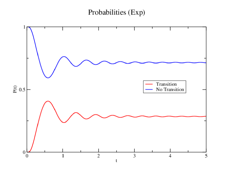
Figure 1: Probabilities of transition or no transition for the function $a_{1}(t)$ in Eq.(28) with $\alpha=20$ and $\beta=1/2$.

After solving the GW equations (5) numerically (double precision) we calculate the above probabilities. Indeed, the probability of finding the system in the $E_{-}$ state with negative PT-norm is zero to machine precision for all $t$. The probabilities of revealing the state to be $E_{0}$ (no transition) or the $E_{+}$ (transition occurring) are shown in the figures. The results are shown in Figure 1 (for ${a_{1}}(t)$ with $\alpha=20$ and $\beta=1/2$) and Figure 2 (for ${a_{2}}(t)$ with $\alpha=2.5$ and $\omega=2.5$). The parameters, of course, can be varied but our numbers were picked to produce behaviors typical of the system. Figure 1 shows the transition/no transition probabilities for the exponential choice above; there are mild oscillations as they approach a limit. In figure 2, we show the corresponding results for the $a_{2}(t)$ choice. In this case, the probabilities show a complex beat structure.

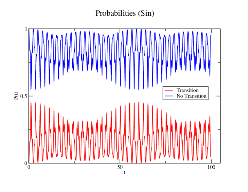
Figure 2: Probabilities of transition or no transition for the function $a_{2}(t)$ in Eq.(28) with $\alpha=2.5$ and $\omega=2.5$.

Our last example is a simple solvable continuum model. Consider the Hermitian Hamiltonian

$$H=1/2\,p^{2}+1/2\,x^{2}+g(t)x$$ (38)

which is a shifted harmonic oscillator with a time-dependent shift. We take $g(0)=0$ so that the linear perturbation turns on at $t=0$. The matrix elements between oscillator states $\langle\phi_{n}|x|\phi_{m}\rangle$ do not vanish when $m=n\pm 1$ and thus transitions between states are induced by this time-dependent perturbation as long as the state indices differ by at most one unit. Will this phenomenon persist if the perturbation is PT-symmetric? Consider

$$H=1/2\,p^{2}+1/2\,x^{2}+ig(t)x,$$ (39)

where again $g(0)=0$. This PT-symmetric Hamiltonian is exactly solvable. The energy eigenvalues are $E_{n}=n+1/2+g(t)^{2}/2$, $n=0,1,2\dots$ with corresponding eigenstates

$$\psi_{n}=\phi_{n}(x+ig)=e^{-g(t)\hat{p}}\phi_{n}(x),$$ (40)

where again the $\phi_{n}(x)$ are the eigenstates of the harmonic oscillator, and $\hat{p}$ is the momentum operator. The ${\cal C}$ operator for this system is

$${\cal C}={\cal P}e^{2g\hat{p}}=e^{-2g\hat{p}}{\cal P}.$$ (41)

Will there be transitions between oscillator states (defined at $t=0$) induced by the perturbation turning on? We already have a selection rule for these transitions which is our Eq.(17). One factor on the right hand side sum is $(e_{n}+e_{m})/2$. In order for the term labeled by $m$ to appear in the sum, it must be that $e_{n}$ and $e_{m}$ have the same sign, either both plus or both minus. Thus, if $n=0$ say (the ground state of the oscillator) then $m$ can only be $0,2,4,\dots$, states with the same PT-norm. However, there is another factor $\langle\psi_{n}|{\cal P}|\dot{\psi}_{m}\rangle$ inside the sum. For the simple system above, we may calculate this factor:

$$\langle\psi_{n}|{\cal P}|\dot{\psi}_{m}\rangle=\langle\phi_{n}|e^{-g\hat{p}}{\cal P}{d\over dt}e^{-g\hat{p}}|\phi_{m}\rangle$$ (42)

$$=-\dot{g}(t)\langle\phi_{n}|e^{-g\hat{p}}e^{+g\hat{p}}{\cal P}\hat{p}|\phi_{m}\rangle$$ (43)

$$=+\dot{g}(t)(-1)^{m}\langle\phi_{n}|\hat{p}|\phi_{m}\rangle.$$ (44)

Hence, immediately in Eq.(17) we have

$$\dot{A}_{n}=0.$$ (45)

The last result follows because the momentum operator, $\hat{p}$, can connect only those states whose quantum numbers differ by at most unity, which violates the selection rule. Thus, for this system, once it is in an eigenstate of energy it cannot transition to a different eigenstate of energy. This effect makes the system entirely trivial and much different from its Hermitian cousin.

One may ask if this non-transition effect persists for more interesting systems, such as the harmonic oscillator with an $ig(t)x^{3}$ perturbation, a system which has been studied but for which there are no analytic results available; the ${\cal C}$ operator has been calculated in perturbation theory. [4] Also, what transitions are allowed for the pure $igx^{3}$ oscillator for which it has been proved that there are all real eigenvalues. [8] Does the selection rule persist in PT-symmetric quantum field theory? If so what restrictions on physical phenomena does it inhibit or allow?

Acknowledgements The work of DG is supported in part by NSF grant PHY-1505565 to Oakland University.

References

- [1] C.M.Bender, Dorje C. Brody and Hugh F. Jones, Phys. Rev. Lett. v89, 270401, 2002.
- [2] The literature on PT-symmetric quantum theory is now vast. Good general references are: Carl M. Bender, Rept. Prog. Theo. Phys.70, 947-1018 (2007) and Carl M. Bender, ArXiv:hep-th/0501180v1, 21 Jan. (2005).
- [3] C.M. Bender, J. Brod, A. Refig and M. Reuter, arXiv:quant-ph/ 0402026v1 3 Feb. (2004).
- [4] C.M. Bender and Hugh. F. Jones, arXiv:hep-th/0405113v1 12 May (2004).
- [5] Jiangbin Gong and Qing-hai Wong, J. Phys.A46, 485302 (2013).
- [6] Carl M. Bender, arXiv:quant-ph/0501052v1 11 Jan. (2005).
- [7] C.M. Bender, D. C. Brode and H. F. Jones, Am. J. Phys., pp 1095-1102 (2003).
- [8] I. Giordanelli and G.M. Graf, arXiv:math-ph:1310.7767v2, 15 Mar. (2014).