Discovering Small Target Sets in Social Networks:
A Fast and Effective Algorithm

Abstract

Given a network represented by a graph $G=(V,E)$, we consider a dynamical process of influence diffusion in $G$ that evolves as follows: Initially only the nodes of a given $S\subseteq V$ are influenced; subsequently, at each round, the set of influenced nodes is augmented by all the nodes in the network that have a sufficiently large number of already influenced neighbors. The question is to determine a small subset of nodes $S$ (a target set) that can influence the whole network. This is a widely studied problem that abstracts many phenomena in the social, economic, biological, and physical sciences. It is known that the above optimization problem is hard to approximate within a factor of $2^{\log^{1-\epsilon}|V|}$, for any $\epsilon>0$. In this paper, we present a fast and surprisingly simple algorithm that exhibits the following features: 1) when applied to trees, cycles, or complete graphs, it always produces an optimal solution (i.e, a minimum size target set); 2) when applied to arbitrary networks, it always produces a solution of cardinality which improves on the previously known upper bound; 3) when applied to real-life networks, it always produces solutions that substantially outperform the ones obtained by previously published algorithms (for which no proof of optimality or performance guarantee is known in any class of graphs).

1 Introduction

Social networks have been extensively investigated by student of the social science for decades (see, e.g., [38]). Modern large scale online social networks, like Facebook and LinkedIn, have made available huge amount of data, thus leading to many applications of online social networks, and also to the articulation and exploration of many interesting research questions. A large part of such studies regards the analysis of social influence diffusion in networks of people. Social influence is the process by which individuals adjust their opinions, revise their beliefs, or change their behaviors as a result of interactions with other people [11]. It has not escaped the attention of advertisers that the process of social influence can be exploited in viral marketing [31]. Viral marketing refers to the spread of information about products and behaviors, and their adoption by people. According to Lately [29], “the traditional broadcast model of advertising-one-way, one-to-many, read-only is increasingly being superseded by a vision of marketing that wants, and expects, consumers to spread the word themselves”. For what interests us, the intent of maximizing the spread of viral information across a network naturally suggests many interesting optimization problems. Some of them were first articulated in the seminal papers [27, 28]. The recent monograph [7] contains an excellent description of the area. In the next section, we will explain and motivate our model of information diffusion, state the problem we are investigating, describe our results, and discuss how they relate to the existing literature.

1.1 The Model

Let $G=(V,E)$ be a graph modeling the network. We denote by $\Gamma_{G}(v)$ and by $d_{G}(v)=|\Gamma_{G}(v)|$, respectively, the neighborhood and the degree of the vertex $v$ in $G$. Let $t:V\to{\mathbb{N}}_{0}=\{0,1,\ldots\}$ be a function assigning thresholds to the vertices of $G$. For each node $v\in V$, the value $t(v)$ quantifies how hard it is to influence node $v$, in the sense that easy-to-influence elements of the network have “low” threshold values, and hard-to-influence elements have “high” threshold values [26].

Definition 1.

Let $G=(V,E)$ be a graph with threshold function $t:V\longrightarrow{\mathbb{N}}_{0}$ and $S\subseteq V$. An activation process in $G$ starting at $S$ is a sequence of vertex subsets ${{\sf Active}}_{G}[S,0]\subseteq{{\sf Active}}_{G}[S,1]\subseteq\ldots\subseteq{{\sf Active}}_{G}[S,\ell]\subseteq\ldots\subseteq V$ of vertex subsets, with ${{\sf Active}}_{G}[S,0]=S$ and

$${{\sf Active}}_{G}[S,\ell]={{\sf Active}}_{G}[S,\ell-1]\cup\Big{\{}u:\,\big{|}\Gamma_{G}(u)\cap{{\sf Active}}_{G}[S,\ell-1]\big{|}\geq t(u)\Big{\}},\mbox{ for $\ell\geq 1$.}$$

A target set for $G$ is set $S\subseteq V$ such that ${{\sf Active}}_{G}[S,\lambda]=V$ for some $\lambda\geq 0$

In words, at each round $\ell$ the set of active nodes is augmented by the set of nodes $u$ that have a number of already activated neighbors greater or equal to $u$’s threshold $t(u)$. The vertex $v$ is said to be activated at round $\ell>0$ if $v\in{{\sf Active}}_{G}[S,\ell]\setminus{{\sf Active}}_{G}[S,\ell-1]$.

In the rest of the paper we will omit the subscript $G$ whenever the graph $G$ is clear from the context.

Example 1.

Consider the tree $T$ in Figure 1. The number inside each circle is the vertex threshold. A possible target set for $T$ is $S=\{v_{1},v_{5},v_{7}\}$. Indeed we have

${{\sf Active}}[S,0]=S=\{v_{1},v_{5},v_{7}\},$

${{\sf Active}}[S,1]=S\cup\{v_{2},v_{3},v_{4},v_{6},v_{8},v_{9}\},$

${{\sf Active}}[S,2]={{\sf Active}}[S,1]\cup\{v_{10}\}=V$

Figure 1: A tree with vertex set $V=\{v_{1},v_{2},\ldots,v_{10}\}$ where the number inside each circle is the vertex threshold. A target set is $S=\{v_{1},v_{5},v_{7}\}$.

The problem we study in this paper is defined as follows:

• Target Set Selection (TSS).
  Instance: A network $G=(V,E)$, thresholds $t:V\rightarrow{\mathbb{N}}_{0}$.
  Problem: Find a target set $S\subseteq V$ of minimum size for $G$.

1.2 The Context and our Results

The Target Set Selection Problem has roots in the general study of the spread of influence in Social Networks (see [7, 23] and references quoted therein). For instance, in the area of viral marketing [22], companies wanting to promote products or behaviors might initially try to target and convince a few individuals who, by word-of-mouth, can trigger a cascade of influence in the network leading to an adoption of the products by a much larger number of individuals. Recently, viral marketing has been also recognised as an important tool in the communication strategies of politicians [4, 30, 37].

The first authors to study problems of spread of influence in networks from an algorithmic point of view were Kempe et al. [27, 28]. However, they were mostly interested in networks with randomly chosen thresholds. Chen [6] studied the following minimization problem: Given a graph $G$ and fixed arbitrary thresholds $t(v)$, $\forall v\in V$, find a target set of minimum size that eventually activates all (or a fixed fraction of) nodes of $G$. He proved a strong inapproximability result that makes unlikely the existence of an algorithm with approximation factor better than $O(2^{\log^{1-\epsilon}|V|})$. Chen’s result stimulated a series of papers [1, 2, 3, 5, 10, 8, 9, 13, 12, 14, 24, 34, 35, 40] that isolated interesting cases in which the problem (and variants thereof) become tractable. A notable absence from the literature on the topic (with the exception of [36, 21]) are heuristics for the Target Set Selection Problem that work for general graphs. This is probably due to the previously quoted strong inapproximability result of Chen [6], that seems to suggest that the problem is hopeless. Providing such an algorithm for general graphs, evaluating its performances and esperimentally validating it on real-life networks, is the main objective of this paper.

Our Results

In this paper, we present a fast and simple algorithm that exhibits the following features:
1) It always produces an optimal solution (i.e, a minimum size subset of nodes that influence the whole network) in case $G$ is either a tree, a cycle, or a complete graph. These results were previously obtained in [6, 34] by means of different ad-hoc algorithms.
2) For general networks, it always produces a target set whose cardinality improves on the upper bound $\sum_{v\in V}\min\left(1,\frac{t(v)}{d(v)+1}\right)$ derived in [16] and obtained in [1] by means of the probabilistic method;
3) In real-life networks it produces solutions that outperform the ones obtained using the algorithms presented in the papers [36, 21], for which, however, no proof of optimality or performance guarantee is known in any class of graphs. The data sets we use, to experimentally validate our algorithm, include those considered in [36, 21].

It is worthwhile to remark that our algorithm, when executed on a graph $G$ for which the thresholds $t(v)$ have been set equal to the nodes degree $d(v)$, for each $v\in V$, it outputs a vertex cover of $G$, (since in that particular case a target set of $G$ is, indeed, a vertex cover of $G$). Therefore, our algorithm appears to be a new algorithm, to the best of our knowledge, to compute the vertex cover of graphs (notice that our algorithm differs from the classical algorithm that computes a vertex cover by iteratively deleting a vertex of maximum degree in the graph). We plan to investigate elsewhere the theoretical performances of our algorithm (i.e., its approximation factor); computational experiments suggest that it performs surprisingly well in practice.

2 The TSS algorithm

In this section we present our algorithm for the TSS problem. The algorithm, given in Figure 2, works by iteratively deleting vertices from the input graph $G$. At each iteration, the vertex to be deleted is chosen as to maximize a certain function. During the deletion process, some vertex $v$ in the surviving graph may remain with less neighbors than its threshold; in such a case $v$ is added to the target set and deleted from the graph while its neighbors’ thresholds are decreased by 1 (since they receive $v$’s influence). It can also happen that the surviving graph contains a vertex $v$ whose threshold has been decreased down to 0 (which means that the deleted nodes are able to activate $v$); in such a case $v$ is deleted from the graph and its neighbors’ thresholds are decreased by 1 (since once $v$ activates, they will receive $v$’s influence).

Algorithm TSS($G$)

Input: A graph $G=(V,E)$ with thresholds $t(v)$ for $v\in V$.

1. $S=\emptyset$

2. $U=V$

3. for each $v\in V$ do

4.           ${\delta}(v)=d(v)$

5.           $k(v)=t(v)$

6.           $N(v)=\Gamma(v)$

7. while $U\neq\emptyset$ do

8.        [Select one vertex and eliminate it from the graph as specified in the following cases]

9.        if there exists $v\in U$ s.t. $k(v)=0$ then

10.              [Case 1: The vertex $v$ is activated by the influence of its neighbors in $V-U$ only;

11.              it can then influence its neighbors in $U$]

12.              for each $u\in N(v)$ do $k(u)=\max(k(u)-1,0)$

13.        else

14.              if there exists $v\in U$ s.t. ${\delta}(v)<k(v)$ then

15.                 [Case 2: The vertex $v$ is added to $S$, since no sufficient neighbors remain

16.                             in $U$ to activate it; $v$ can then influence its neighbors in $U$]

17.                 $S=S\cup\{v\}$

18.                 for each $u\in N(v)$ do $k(u)=k(u)-1$

19.              else

20.                 [Case 3: The vertex $v$ will be influenced by some of its neighbors in $U$]

21.                 $v={\tt argmax}_{u\in U}\left\{\frac{k(u)}{\delta(u)(\delta(u)+1)}\right\}$

22.        [Remove the selected vertex $v$ from the graph]

23.        for each $u\in N(v)$ do

24.                    ${\delta}(u)={\delta}(u)-1$

25.                    $N(u)=N(u)-\{v\}$

26.        $U=U-\{v\}$

Figure 2: The TSS algorithm.

Example 1(cont.) Consider the tree $T$ in Figure 1. A possible run of the algorithm $TSS(T)$ removes the nodes from $T$ in the order of the list below, where we also indicate for each vertex which among Cases 1, 2, and 3 applies:

Iteration	1	2	3	4	5	6	7	8	9	10
vertex	$v_{10}$	$v_{9}$	$v_{8}$	$v_{7}$	$v_{6}$	$v_{5}$	$v_{4}$	$v_{3}$	$v_{2}$	$v_{1}$
Case	3	3	3	2	3	2	1	3	3	2

Hence the algorithms outputs the set $\{v_{1},v_{5},v_{7}\}$ which is a target set for $T$.

Before starting the deletion process, the algorithm initialize three variables for each node:

• ${\delta}(v)$ to the initial degree of node $v$,

• $k(v)$ to the initial threshold of node $v$, and

• $N(v)$ the initial set of neighbors of node $v$.

In the rest of the paper, we use the following notation. We denote by $n$ the number of nodes in $G$, that is, $n=|V|$. Moreover we denote:

• By $v_{i}$ the vertex that is selected during the $n-i+1$-th iteration of the while loop in TSS($G$), for $i=n,\ldots,1$;

• by $G(i)$ the graph induced by $V_{i}=\{v_{i},\ldots,v_{1}\}$

• by $\delta_{i}(v)$ the value of $\delta(v)$ as updated at the beginning of the $(n-i+1)-th$ iteration of the while loop in TSS($G$).

• by $N_{i}(v)$ the set $N(v)$ as updated at the beginning of the $(n-i+1)-th$ iteration of the while loop in TSS($G$), and

• by $k_{i}(v)$ the value of $k(v)$ as updated at the beginning of the $(n-i+1)-th$ iteration of the while loop in TSS($G$).

For the initial value $i=n$, the above values are those of the input graph $G$, that is: $G(n)=G$, $\delta_{n}(v)=d(v)$, $N_{n}(v)=\Gamma(v)$, $k_{n}(v)=t(v)$, for each vertex $v$ of $G$.

We start with two technical Lemmata which will be useful in the rest of the paper.

Lemma 1.

Consider a graph $G$. For any $i=n,\ldots,1$ and $u\in V_{i}$, it holds that

$$\Gamma_{G(i)}(u)=N_{i}(u)\quad\mbox{ and }\quad d_{G(i)}(u)=\delta_{i}(u).$$ (1)

Proof.

For $i=n$ we have $d_{G(n)}(u)=d_{G}(u)=\delta_{n}(u)$ and $\Gamma_{G(n)}(u)=\Gamma_{G}(u)=N_{n}(u)$ for any $u\in V_{n}=V$.
Suppose now that the equalities hold for some $i\leq n$. The graph $G(i-1)$ corresponds to the subgraph of $G(i)$ induced by $V_{i-1}=V_{i}-\{v_{i}\}$. Hence

$$\Gamma_{G(i-1)}(u)=\Gamma_{G(i)}(u)-\{v_{i}\},$$

and

$$d_{G(i-1)}(u)=\begin{cases}{d_{G(i)}(u)-1}&{\mbox{if $u\in\Gamma_{G(i)}(v_{i})$,}}\\ {d_{G(i)}(u)}&{\mbox{otherwise.}}\end{cases}$$

We deduce that the desired equalities hold for $i-1$ by noticing that the algorithm uses the same rules to get

$$N_{i-1}(u)=N_{i}(u)-\{v_{i}\}$$

and

$$\delta_{i-1}(u)=\begin{cases}{\delta_{i}(u)-1}&{\mbox{if $u\in N_{i}(v_{i})=\Gamma_{G(i)}(v_{i}),$}}\\ {\delta_{i}(u)}&{\mbox{otherwise}.}\end{cases}$$

∎

Lemma 2.

For any $i>1$, if $S^{(i-1)}$ is a target set for $G(i-1)$ with thresholds $k_{i-1}(u)$, for $u\in V_{i-1}$, then

$$S^{(i)}=\begin{cases}{S^{(i-1)}\cup\{v_{i}\}}&{\mbox{if $k_{i}(v_{i})>\delta_{i}(v_{i})$}}\\ {S^{(i-1)}}&{\mbox{otherwise}}\end{cases}$$ (2)

is a target set for $G(i)$ with thresholds $k_{i}(u)$, for $u\in V_{i}$.

Proof.

Let us first notice that, according to the algorithm $TSS$, for each $u\in V_{i-1}$ we have

$$k_{i-1}(u)=\begin{cases}{\max(k_{i}(u)-1,0)}&{\mbox{if $u\in N_{i}(v_{i})$ and ($k_{i}(v_{i})=0$ or $k_{i}(v_{i})>\delta_{i}(v_{i})$)}}\\ {k_{i}(u)}&{\mbox{otherwise.}}\end{cases}$$ (3)

• If $k_{i}(v_{i})=0$, then $v_{i}\in{{\sf Active}}_{G(i)}[S^{(i)},1]$ whatever $S^{(i)}\subseteq V_{i}-\{v_{i}\}$. Hence, by the equation (3), any target set $S^{(i-1)}$ for $G(i-1)$ is also a target set for $G(i)$.

• If $k_{i}(v_{i})>\delta_{i}(v_{i})$ then $S^{(i)}=S^{(i-1)}\cup\{v_{i}\}$ and $k_{i-1}(u)=k_{i}(u)-1$ for each $u\in N_{i}(v_{i})$. It follows that for any $\ell\geq 0$,

  $${{\sf Active}}_{G(i)}[S^{(i-1)}\cup\{v_{i}\},\ell]-\{v_{i}\}={{\sf Active}}_{G(i-1)}[S^{(i-1)},\ell].$$

  Hence, ${{\sf Active}}_{G(i)}[S^{(i)},\ell]={{\sf Active}}_{G(i-1)}[S^{(i-1)},\ell]\cup\{v_{i}\}.$

• Let now $1\leq k_{i}(v_{i})\leq\delta_{i}(v_{i})$. We have that $k_{i-1}(u)=k_{i}(u)$ for each $u\in V_{i-1}$. If $S^{(i-1)}$ is a target set for $G(i-1)$, by definition there exists an integer $\lambda$ such that ${{\sf Active}}_{G(i-1)}[S^{(i-1)},\lambda]=V_{i-1}$. We then have $V_{i-1}\subseteq{{\sf Active}}_{G(i)}[S^{(i-1)},\lambda]$ which implies ${{\sf Active}}_{G(i)}[S^{(i-1)},\lambda+1]=V_{i}$.

∎

We can now prove the main result of this section.

Theorem 1.

For any graph $G$ and threshold function $t$, the algorithm TSS($G$) outputs a target set for $G$.

Proof.

Let $S$ be the output of the algorithm $TSS(G)$. We show that for each $i=1,\ldots,n$ the set $S\cap\{v_{i},\ldots,v_{1}\}$ is a target set for the graph $G(i)$, assuming that each vertex $u$ in $G(i)$ has threshold $k_{i}(u)$. The proof is by induction on the number $i$ of nodes of $G(i)$.
If $i=1$ then the unique vertex $v_{1}$ in $G(1)$ either has threshold $k_{1}(v_{1})=0$ and $S\cap\{v_{1}\}=\emptyset$ or the vertex has positive threshold $k_{1}(v_{1})>{\delta}_{1}(v_{1})=0$ and $S\cap\{v_{1}\}=\{v_{1}\}$.
Consider now $i>1$ and suppose the algorithm be correct on $G(i-1)$, that is, $S\cap\{v_{i-1},\ldots,v_{1}\}$ is a target set for $G(i-1)$ with threshold function $k_{i-1}$. We notice that in each among Cases 1, 2 and 3, the algorithm updates the thresholds and the target set according to Lemma 2. Hence, the algorithm is correct on $G(i)$ with threshold function $k_{i}$. The theorem follows since $G(n)=G$. ∎

It is possible to see that the TSS algorithm can be implemented in such a way to run in $O(|E|\log|V|)$ time. Indeed we need to process the nodes $v\in V$ according to the metric $t(v)/(d(v)(d(v)+1))$, and the updates that follow each processed node $v\in V$ involve at most the $d(v)$ neighbors of $v$.

3 Estimating the Size of the Solution

In this section we prove an upper bound on the size of the target set obtained by the algorithm TSS($G$) for any input graph $G$. Our bound, given in Theorem 2, improves on the bound $\sum_{v\in V}\min\left(1,\frac{t(v)}{d(v)+1}\right)$ given in [1] and [16]. Moreover, the result in [1] is based on the probabilistic method and an effective algorithm results only by applying suitable derandomization steps.

Theorem 2.

Let $G$ be a connected graph with at least 3 nodes and threshold function $t:V\to{\mathbb{N}}_{0}$. The algorithm TSS($G$) outputs a target set $S$ of size

$$|S|\leq\sum_{v\in\{u\,|\,u\in V^{(2)}\,\lor\,t(u)\neq 1\}}\min\left(1,\frac{t(v)}{d^{(2)}(v){+}1}\right),$$ (4)

where $V^{(2)}{=}\{v\,|\,v\in V,\,d(v){\geq}2\}$ and $d^{(2)}(v){=}|\{u\in\Gamma(v)\,|\,u\in V^{(2)}\,\lor\,t(u){\neq}1\}|$.

Proof.

For each $i=1,\ldots,n$, define

• $\delta^{(2)}_{i}(v)=|\{u\in N_{i}(v)\,|\,u\in V^{(2)}\,\lor\,t(u)\neq 1\}|$;
  

• $I_{i}=\left\{v\,{|}\,v\in V_{i}-V^{(2)},\,k_{i}(v)>\delta_{i}(v)\right\}$,

• $W(G(i))=\sum_{v\in V_{i}\cap V^{(2)}}\min\left(1,\frac{k_{i}(v)}{\delta^{(2)}_{i}(v)+1}.\right)+|I_{i}|.$

We prove that

$$|S\cap V_{i}|\leq W(G(i)),$$ (5)

for each $i=1,\ldots,n$. The bound (4) on $S$ follows recalling that $G(n)=G$ and
$I_{n}=\left\{v\,{|}\,v\not\in V^{(2)},\,t(v)=k(v)>{\delta}(v)=d(v)=1\right\}$.

The proof is by induction on $i$. If $i=1$, the claim follows noticing that

$$|S\cap\{v_{1}\}|{=}\begin{cases}{0}&{\mbox{if $k_{1}(v_{1}){=}0$}}\\ {1}&{\mbox{if $k_{1}(v_{1}){\geq}1$}}\end{cases}\quad\mbox{ and }\quad W(G(1)){=}\begin{cases}{0}&{\mbox{if $k_{1}(v_{1}){=}0$ and $v_{1}{\in}V^{(2)}$}}\\ {1}&{\mbox{otherwise.}}\end{cases}$$

Assume now (5) holds for $i-1\geq 1$, and consider $G(i)$ and the node $v_{i}$. We have

$$|S\cap\{v_{i},\ldots,v_{1}\}|=|S\cap\{v_{i}\}|+|S\cap\{v_{i-1},\ldots,v_{1}\}|\leq|S\cap\{v_{i}\}|+W(G(i-1)).$$

We show now that

$$W(G(i))\geq W(G(i-1))+|S\cap\{v_{i}\}|.$$

We first notice that $W(G(i))-W(G(i-1))$ can be written as

$$\sum_{v\in V_{i}\cap V^{(2)}}\min\left(1,\frac{k_{i}(v)}{\delta^{(2)}_{i}(v)+1}\right){+}|I_{i}|{-}\sum_{v\in V_{i-1}\cap V^{(2)}}\min\left(1,\frac{k_{i-1}(v)}{\delta^{(2)}_{i-1}(v)+1}\right){-}|I_{i-1}|$$

We notice that $k_{i}(v)-1\leq k_{i-1}(v)\leq k_{i}(v)$ and $\delta_{i}(v)-1\leq\delta_{i-1}(v)\leq\delta_{i}(v)$, for each neighbor $v$ of $v_{i}$ in $G(i)$, and that threshold and degree remain unchanged for each other node in $G(i-1)$. Therefore, we get

$$W(G(i))-W(G(i-1))\geq|I_{i}| - |I_{i-1}|$$ (6)

$$+\sum_{v\in N_{i}(v_{i})\cap V^{(2)}\atop k_{i}(v)\leq\delta^{(2)}_{i}(v)}\left(\frac{k_{i}(v)}{\delta^{(2)}_{i}(v)+1}-\frac{k_{i-1}(v)}{\delta^{(2)}_{i-1}(v)+1}\right)$$

$$+\begin{cases}\min\left(1,\frac{k_{i}(v_{i})}{\delta^{(2)}_{i}(v_{i})+1}\right)&{\mbox{if }d(v_{i})\geq 2}\\ 0&\mbox{otherwise}.\end{cases}$$

We distinguish three cases according to those in the algorithm TSS($G$).

I)

Suppose that Case 1 of the Algorithm TSS holds; i.e. $k_{i}(v_{i})=0$. Recall that the Algorithm TSS($G$) updates the the values of ${\delta}(u)$ and $k(u)$ for each node in $V_{i}$ as follows:

$${\delta}_{i-1}(u){=}\begin{cases}{{\delta}_{i}(u){-}1}&{\mbox{if $u{\in}N(v_{i})$}}\\ {{\delta}_{i}(u)}&{\mbox{otherwise,}}\end{cases}\quad k_{i-1}(u){=}\begin{cases}{k_{i}(u){-}1}&{\mbox{if $u{\in}N(v_{i})$, $k_{i}(u){>}0$}}\\ {k_{i}(u)}&{\mbox{otherwise.}}\end{cases}$$ (7)

By b), (7) and being $k_{i}(v_{i})=0$, we immediately get $I_{i-1}=I_{i}$. Hence, from (6) we have

$$W(G(i))-W(G(i-1))\geq\sum_{v\in N_{i}(v_{i})\cap V^{(2)}\atop k_{i}(v)\leq\delta^{(2)}_{i}(v)}\left(\frac{k_{i}(v)}{\delta^{(2)}_{i}(v)+1}-\frac{k_{i-1}(v)}{\delta^{(2)}_{i-1}(v)+1}\right)\geq 0,$$

where the last inequality is implied by (7). Since we know that in Case 1 the selected node $v_{i}$ is not part of $S$, we get the desired inequality $W(G(i))-W(G(i-1))\geq|S\cap\{v_{i}\}|$.

II)

Suppose that Case 2 of the algorithm holds; i.e. $k_{i}(v_{i})\geq\delta_{i}(v_{i})+1$ and $k(v)>0$ for each $v\in V_{i}$. The Algorithm TSS($G$) updates the values of ${\delta}(u)$ and $k(u)$ for each node $u\in V_{i-1}$ as in (7). Hence, we have

$$I_{i-1}=\begin{cases}{I_{i}}&{\mbox{if $d(v_{i})\geq 2$}}\\ {I_{i}-\{v_{i}\}}&{{\mbox{otherwise}}}\end{cases}$$

and, using this case assumption, equation (6) becomes

$$W(G(i))-W(G(i-1))\geq 1+\sum_{v\in N_{i}(v_{i})\cap V^{(2)}\atop k_{i}(v)\leq\delta^{(2)}_{i}(v)}\left(\frac{k_{i}(v)}{\delta^{(2)}_{i}(v)+1}-\frac{k_{i-1}(v)}{\delta^{(2)}_{i-1}(v)+1}\right)\geq 1.$$

Since in Case 2 $v_{i}$ is part of the output $S$, we get $W(G(i))-W(G(i-1))\geq 1=|S\cap\{v_{i}\}|$.

III)

Suppose that Case 3 of the algorithm holds. We know that:

• $1\leq k_{i}(v)\leq{\delta}_{i}(v)$, for each $v\in V_{i}$;

• $I_{i}=\emptyset$—by (i) above;

• $\frac{k_{i}(v_{i})}{{\delta}_{i}(v_{i})(\delta_{i}(v_{i})+1)}\geq\frac{k_{i}(v)}{{\delta}_{i}(v)({\delta}_{i}(v)+1)}$, for each $v\in V_{i}$;

• for each $v\in V_{i-1}$, $k_{i-1}(u)=k_{i}(u)$ and ${\delta}_{i-1}(u)=\begin{cases}{{\delta}_{i}(u){-}1}&{\mbox{ if $u{\in}N(v_{i})$}}\\ {{\delta}_{i}(u)}&{\mbox{ otherwise.}}\end{cases}$

We distinguish three cases on the value of $d(v_{i})$ and $\delta_{i}(v_{i})$:

• Suppose first $d(v_{i})\geq\delta_{i}(v_{i})\geq 2$. We have $\delta_{i}(v)\geq 2$, for each $\ v\in V_{i}$. Otherwise, by (i) we would get $\delta_{i}(v)=k_{i}(v)=1$ and, as a consequence

  $$\frac{k_{i}(v)}{\delta_{i}(v)(\delta_{i}(v)+1)}=1/2,\quad\mbox{ while }\frac{k_{i}(v_{i})}{\delta_{i}(v_{i})(\delta_{i}(v_{i})+1)}\leq\frac{1}{\delta_{i}(v_{i})+1}\leq 1/3,$$

  contradicting (iii). Therefore, by b) $I_{i-1}=\emptyset$ and $\delta^{(2)}_{i}(v)=\delta_{i}(v)$, for each $v\in V_{i}$. This, (ii), and (6) imply

  $$W(G(i))-W(G(i-1)) \geq \sum_{v\in N_{i}(v_{i})\atop k_{i}(v)\leq\delta_{i}(v)}\left(\frac{k_{i}(v)}{\delta_{i}(v)+1}-\frac{k_{i}(v)}{\delta_{i}(v)}\right)+\frac{k_{i}(v_{i})}{\delta_{i}(v_{i})+1}$$

  $$= \frac{k_{i}(v_{i})}{\delta_{i}(v_{i})+1}-\sum_{v\in N_{i}(v_{i})\atop k_{i}(v)\leq\delta_{i}(v)}\frac{k_{i}(v)}{\delta_{i}(v)(\delta_{i}(v)+1)}.$$

  As a consequence, by using (iii) and recalling that $v_{i}\notin S$ we get

  $$W(G(i))-W(G(i-1))\geq\frac{k_{i}(v_{i})}{\delta_{i}(v_{i})+1}-\frac{k_{i}(v_{i})}{\delta_{i}(v_{i})+1}=0=|S\cap\{v_{i}\}|.$$

• Assume now $d(v_{i})\geq 2$ and $\delta_{i}(v_{i})=1$. Let $u$ be the neighbor of $v_{i}$ in $G(i)$.
  If $d(u)\geq 2,$ then $u\notin I_{i-1}$ and, by (ii), $I_{i-1}=I_{i}=\emptyset.$ By (6), we obtain

  $$W(G(i)){-}W(G(i{-}1)) \geq \left(\frac{k_{i}(u)}{\delta^{(2)}_{i}(u)+1}{-}\frac{k_{i-1}(u)}{\delta^{(2)}_{i-1}(u)+1}\right){+}\min\left(1,\frac{k_{i}(v_{i})}{\delta^{(2)}_{i}(v_{i})+1}\right)$$

  $$= \left(\frac{k_{i}(u)}{\delta^{(2)}_{i}(u)+1}{-}\frac{k_{i}(u)}{\delta^{(2)}_{i}(u)}\right){+}1/2$$

  $$= 1/2-\frac{k_{i}(u)}{\delta^{(2)}_{i}(u)(\delta^{(2)}_{i}(u)+1)}$$

  $$\geq 1/2-\frac{1}{\delta^{(2)}_{i}(u)+1}\geq 0=|S\cap\{v_{i}\}|.$$

  
  

  If $d(u)=1$ then by (i) $1\leq k_{i}(u)\leq t(u)\leq d(u)$ and we have $t(u)=1$. Moreover, by (iv) ${\delta}_{i-1}(u)=0$, ${\delta}^{(2)}_{i}(v_{i})=0$ and $k_{i-1}(u)=k_{i}(u)\geq 1$. Hence $u\in I_{i-1}.$ Recalling that $I_{i}=\emptyset$, we get $I_{i-1}=\{u\}.$ As a consequence, (6) becomes

  $$W(G(i))-W(G(i-1)) \geq |I_{i}|-|I_{i-1}|+0+\min\left(1,\frac{k_{i}(v_{i})}{\delta^{(2)}_{i}(v_{i})+1}\right)$$

  $$= 0=|S\cap\{v_{i}\}|.$$

• Suppose finally $d(v_{i})=1$. Let $u$ be the unique neighbor of $v_{i}$ in $G(i)$
  If $d(u)\geq 2$, then $u\notin I_{i-1}$ and, by (ii), $I_{i-1}=I_{i}=\emptyset.$ Moreover, by (i) we know that $1\leq k_{i}(v_{i})\leq t(v_{i})\leq d(v_{i})$ and we have $t(v_{i})=1$. Hence $\delta^{(2)}_{i}(u)=\delta^{(2)}_{i-1}(u)$. By (6), we obtain

  $$W(G(i)){-}W(G(i{-}1))\geq 0+\left(\frac{k_{i}(u)}{\delta^{(2)}_{i}(u)+1}{-}\frac{k_{i-1}(u)}{\delta^{(2)}_{i-1}(u)+1}\right)=0=|S\cap\{v_{i}\}|.$$

  Finally, the case $d(u)\leq 1$ can hold only if the input graph $G$ has a connected component consisting of two nodes. This is excluded by the theorem hypothesis.

∎

Remark 1.

We notice that the bound in Theorem 2 improves on the previously known bound $\sum_{v\in V}\min\left(1,t(v)/(d(v)+1)\right)$ given in [1, 16]. Indeed we are able to show that for any graph

$$\sum_{v\in\{u\,|\,u\in V^{(2)}\,\lor\,t(u)\neq 1\}}\min\left(1,\frac{t(v)}{d^{(2)}(v){+}1}\right)\leq\sum_{v\in V}\min\left(1,\frac{t(v)}{d(v)+1}\right).$$ (8)

In order to prove (8), we first notice that the difference between the two bounds can be written as,

$$\sum_{v\in V}\min\left(1,\frac{t(v)}{d(v)+1}\right)-\sum_{v\in\{u\,|\,u\in V^{(2)}\,\lor\,t(u)\neq 1\}}\min\left(1,\frac{t(v)}{d^{(2)}(v){+}1}\right)=$$

$$\sum_{v\in V^{(2)}}\min\left(1,\frac{t(v)}{d(v){+}1}\right){+}\sum_{v\notin V^{(2)}}\min\left(1,\frac{t(v)}{2}\right){-}\sum_{v\in V^{(2)}}\min\left(1,\frac{t(v)}{d^{(2)}(v){+}1}\right){+}\sum_{v\notin V^{(2)}\atop t(v)>1}{1}=$$

$$\sum_{v\in V^{(2)}}\min\left(1,\frac{t(v)}{d(v){+}1}\right){+}\sum_{v\notin V^{(2)}\atop t(v)=1}{1/2}-\sum_{v\in V^{(2)}}\min\left(1,\frac{t(v)}{d^{(2)}(v){+}1}\right)\geq$$

$$\sum_{v\in V^{(2)}\atop t(v)\leq d(v)}\frac{t(v)}{d(v)+1}+\sum_{v\notin V^{(2)}\atop t(v)=1}{1/2}-\sum_{v\in V^{(2)}\atop t(v)\leq d(v)}\min\left(1,\frac{t(v)}{d^{(2)}(v)+1}\right)\geq$$

$$\sum_{v\in V^{(2)}\atop t(v)\leq d(v)}\left(\frac{t(v)}{d(v)+1}+{\frac{d(v)-d^{(2)}(v)}{2}}\right)-\sum_{v\in V^{(2)}\atop t(v)\leq d(v)}\min\left(1,\frac{t(v)}{d^{(2)}(v)+1}\right),$$

where the last inequality is due to the fact that

$$\sum_{v\notin V^{(2)}\atop t(v)=1}{1/2}=\sum_{v\in V^{(2)}}{\frac{d(v)-d^{(2)}(v)}{2}}\geq\sum_{v\in V^{(2)}\atop t(v)\leq d(v)}{\frac{d(v)-d^{(2)}(v)}{2}}$$

that is, we are aggregating the contribution of each node, having both degree and threshold equal to $1$, to that of its unique neighbor.

Now let us consider the contribution of each $v\in V^{(2)}$, such that $t(v)\leq d(v)$, to the equation above. If $d(v)=d^{(2)}(v)$, then clearly the contribution of $v$ is zero. If $d(v)-d^{(2)}(v)\geq 2$ then the contribution of $v$ is

$$\frac{t(v)}{d(v)+1}+{\frac{d(v)-d^{(2)}(v)}{2}}-\min\left(1,\frac{t(v)}{d^{(2)}(v)+1}\right)\geq\frac{t(v)}{d(v)+1}+1-1\geq 0$$

Finally, if $d(v)-d^{(2)}(v)=1$ we have

$$\frac{t(v)}{d(v)+1}+{1/2}-\min\left(1,\frac{t(v)}{d(v)}\right)=\frac{t(v)}{d(v)+1}+{1/2}-\frac{t(v)}{d(v)}=\frac{2(d(v)-t(v))}{2d(v)(d(v)+1)}\geq 0.$$

In each case the contribution of $v$ is non negative and (8) holds.

Furthermore it is worth to notice that our bound can give a dramatic improvement with respect to one in [1, 16]. As an example consider the star graph on $n$ nodes with center $c$ given in Figure 3 and thresholds equal to 1 for each leaf node and to $t(c)\leq n$ for the center node $c$. The ratio of the bound in [1, 16] to the one in this paper is

$$\frac{\sum_{v\in V}\min\left(1,\frac{t(v)}{(d(v)+1)}\right)}{\sum_{v\in\{u\,|\,u\in V^{(2)}\,\lor\,t(u)\neq 1\}}\min\left(1,\frac{t(v)}{d^{(2)}(v){+}1}\right)}=\frac{\frac{t(c)}{n}+\frac{n-1}{2}}{1+0}\geq\frac{n-1}{2}.$$

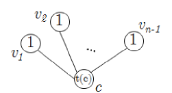
Figure 3: A star graph with $n$ nodes. The bound in [1, 16] provides a target set of size $\frac{t(c)}{n}+\frac{n-1}{2}$ while the bound in Theorem 2 is $1$. In this specific case the bound of Theorem 2 is tight, the optimal target set consists of the center node $c$.

4 Optimality Cases

In this section, we prove that our algorithm TSS provides a unified setting for several results, obtained in the literature by means of different ad hoc algorithms. Trees, cycles and cliques are among the few cases known to admit optimal polynomial time algorithms for the TSS problem [6, 34]. In the following, we prove that our algorithm TSS provides the first unifying setting for all these cases.

Theorem 3.

The algorithm TSS($T$) returns an optimal solution whenever the input graph $T$ is a tree.

Proof.

Let $T=(V,E)$ and $n=|V|$. We recall that for $i=1,\ldots,n$: $v_{i}$ denotes the node selected during the $n-i+1$-th iteration of the while loop in TSS, $T(i)$ is the forest induced by the set $V_{i}=\{v_{i},\ldots,v_{1}\}$, and $\delta_{i}(v)$ and $k_{i}(v)$ are the degree and threshold of $v$, for $v\in V_{i}$. Let $S$ be the target set produced by the algorithm TSS($T$). We prove by induction on $i$ that

$$|S\cap\{v_{i},\ldots,v_{1}\}|=|S^{*}_{i}|,$$ (9)

where $S^{*}_{i}$ represents an optimal target set for the forest $T(i)$ with threshold function $k_{i}$. For $i=1$, it is immediate that for the only node $v_{1}$ in $F(1)$ one has

$$S\cap\{v_{1}\}=S^{*}_{1}=\begin{cases}{\emptyset}&{\mbox{ if }k_{1}(v_{1})=0}\cr{\{v_{1}\}}&{\mbox{ otherwise. }}\end{cases}$$

Suppose now (9) true for $i-1$ and consider the tree $T(i)$ and the selected node $v_{i}$.

1. Assume first that $k_{i}(v_{i})=0$. We get

   $$|S\cap\{v_{i},\ldots,v_{1}\}|=|S\cap\{v_{i-1},\ldots,v_{1}\}|=|S^{*}_{i-1}|\leq|S^{*}_{i}|$$

   and the equality (9) holds for $i$.

2. Assume now that $k_{i}(v_{i})\geq\delta_{i}(v_{i})+1$. Clearly, any solution for $T(i)$ must include node $v_{i}$, otherwise it cannot be activated. This implies that

   $$|S^{*}_{i}|=1+|S^{*}_{i-1}|=1+|S\cap\{v_{i-1},\ldots,v_{1}\}|=|S\cap\{v_{i},\ldots,v_{1}\}|$$

   and (9) holds for $i$.

3. Finally, suppose that $v_{i}={\tt argmax}_{i\geq j\geq 1}\left\{{k_{i}(v_{j})}/{(\delta_{i}(v_{j})(\delta_{i}(v_{j})+1))}\right\}$ (cfr. line 21 of the algorithm). In this case each leaf $v_{j}$ in $T(i)$ has

   $$\frac{k_{i}(v_{\ell})}{\delta_{i}(v_{\ell})(\delta_{i}(v_{\ell})+1)}=\frac{1}{2}$$

   while each internal node $v_{\ell}$ has

   $$\frac{k_{i}(v_{\ell})}{\delta_{i}(v_{\ell})(\delta_{i}(v_{\ell})+1)}\leq\frac{1}{\delta_{i}(v_{\ell})+1}\leq\frac{1}{3}.$$

   Hence, the node $v_{i}$ must be a leaf in $T(i)$ and has $k_{i}(v_{i})=\delta_{i}(v_{i})=1$. Hence $|S\cap\{v_{i},\ldots,v_{1}\}|=|S\cap\{v_{i-1},\ldots,v_{1}\}|=|S^{*}_{i-1}|\leq|S^{*}_{i}|$. aaaaaaaaa∎

Theorem 4.

The algorithm TSS($C$) outputs an optimal solution whenever the input graph $C$ is a cycle.

Proof.

If the first selected node $v_{n}$ has threshold 0 then clearly $v_{n}\not\in S^{*}$ for any optimal solution $S^{*}$.
If the threshold of $v_{n}$ is larger than its degree then clearly $v_{n}\in S^{*}$ for any optimal solution $S^{*}$. In both cases $v_{n}\in{{\sf Active}}[S^{*},1]$ and its neighbors can use $v_{n}$’s influence; that is, the algorithm correctly sets $k_{n-1}=\max(k_{n}-1,0)$ for these two nodes.
If threshold of each node $v\in V$ is $1\leq t(v)\leq d(v)$, we get that during the first iteration of the algorithm TSS($C$), the selected node $v_{n}$ satisfies Case 3 and has $t(v_{n})=2$ if at least one of the nodes in $C$ has threshold $2$, otherwise $t(v_{n})=1$. Moreover, it is not difficult to see that there exists an optimal solution $S^{*}$ for $C$ such that $S^{*}\cap\{v_{n}\}=\emptyset$.
In each case, the result follows by Theorem 3, since the remaining graph is a path on nodes $v_{n-1},\ldots,v_{1}$. ∎

Theorem 5.

Let $K=(V,E)$ be a clique with $V=\{u_{1},\ldots,u_{n}\}$ and $t(u_{1})\leq\ldots\leq t(u_{n-m})<n\leq t(u_{n-m+1})\leq\ldots\leq t(u_{n})$. The algorithm TSS($K$) outputs an optimal target set of size

$$m+\quad\max_{\mathclap{1\leq j\leq n-m}}\quad\max(t(u_{j})-m-j+1,0).$$ (10)

Proof.

It is well known that there exists an optimal target set $S^{*}$ consisting of the $|S^{*}|$ nodes of higher threshold [34]. Being $S^{*}$ a target set, we know that each node in the graph $K$ must activate. Therefore, for each $u\in V$ there exists some iteration $i\geq 0$ such that $u\in{{\sf Active}}[S,i]$. Assume $V=\{u_{1},\ldots,u_{n}\}$ and

$$t(u_{1})\leq\ldots\leq t(u_{n-m})<n\leq t(u_{n-m+1})\leq\ldots\leq t(u_{n}).$$

Since the thresholds are non decreasing with the node index, it follows that:

• for each $j\geq n-m+1$, the node $u_{j}$ has threshold $t(u_{j})\geq n$ and $u_{j}\in S^{*}$ must hold. Hence, $|S^{*}|\geq m$;

• for each $j\leq n-|S^{*}|$, the node $u_{j}$ activates if it gets, in addition to the influence of its $m$ neighbors with threshold larger than $n-1$, the influence of at least $t(u_{j})-m$ other neighbors, hence we have that

  $$t(u_{j})-m\leq j-1+(|S^{*}|-m)$$

  must hold;

• for each $j=n-|S^{*}|+1,\ldots,n-m$, we have

  $$t(u_{j})-m-j+1\leq(n-1)-m-(n-|S^{*}|+1)+1=|S^{*}|-m+1.$$

Summarizing, we get,

$$|S^{*}|\geq m+\quad\max_{{1\leq j\leq n-m}}\quad\max\left(t(u_{j})-m-j+1,0\right).$$

We show now that the algorithm TSS outputs a target set $S$ whose size is upper bounded by the value in (10). Notice that, in general, the output $S$ does not consist of the nodes having the highest thresholds.

Consider the residual graph $K(i)=(V_{i},E_{i})$, for some $1\leq i\leq n$. It is easy to see that for any $u_{j},u_{s}\in V_{i}$ it holds

• 1) $\delta_{i}(u_{j})=i$;
  2) if $j<s$ then $k_{i}(u_{j})\leq k_{i}(u_{s})$;
  3) if $t(u_{j})\geq n$ then $k_{i}(u_{j})\geq i$,
  4) if $t(u_{j})<n$ then $k_{i}(u_{j})\leq i$.

W.l.o.g. we assume that at any iteration of algorithm TSS if the node to be selected is not unique then the tie is broken as follows (cfr. point 2) above):

• If Case 1 holds then the selected node is the one with the lowest index,

• if either Case 2 or Case 3 occurs then the selected node is the one with the largest index.

Clearly, this implies that $K(i)$ contains $i$ nodes with consecutive indices among $u_{1},\ldots,u_{n}$, that is,

$$V_{i}=\left\{u_{\ell_{i}},u_{\ell_{i}+1},\ldots,u_{r_{i}}\right\}$$ (11)

for some $\ell_{i}\geq 1$ and $r_{i}=\ell_{i}+i-1$.

Let $h=n-m$. We shall prove by induction on $i$ that, for each $i=n,\ldots,1$, at the beginning of the $n-i+1$-th iteration of the while loop in TSS($K$), it holds

$$|S\cap V_{i}|\leq\begin{cases}{(r_{i}-h)+\max_{\begin{subarray}{c}\ell_{i}\leq j\leq h\end{subarray}}\max(k_{i}(u_{j})-(r_{i}-h)-j+\ell_{i},\,0)}&{\mbox{ if $r_{i}>h$,}}\\ {\max_{\begin{subarray}{c}\ell_{i}\leq j\leq r_{i}\end{subarray}}\max(k_{i}(u_{j})-j+\ell_{i},\,0)}&{\mbox{ if $r_{i}\leq h$.}}\end{cases}$$ (12)

The upper bound (10) follows when $i=n$; indeed $K(n)=K$ and $|S|=|S\cap V(n)|$.
For $i=1$, $K(1)$ is induced by only one node, let say $u$, and

$$|S\cap\{u\}|=\begin{cases}{1}&{\mbox{\ \ if $k_{1}(u)\geq 1$,}}\\ {0}&{\mbox{\ \ if $k_{1}(u)=0$.}}\end{cases}$$

proving that the bound holds in this case.
Suppose now (12) true for some $i-1\geq 1$ and consider the $n-i+1$-th iteration of the algorithm TSS. Let $v$ be the node selected by algorithm TSS at the $n-i+1$-th iteration. We distinguish three cases according to the cases of the algorithm TSS($G$).

Case 1: $k_{i}(v)=0$.   By i) and (11), one has $v=u_{\ell_{i}}$, $\ell_{i-1}=\ell_{i}+1$ and $r_{i-1}=r_{i}$. Moreover, $k_{i}(u_{j})=k_{i-1}(u_{j})+1$ for each $u_{j}\in V_{i-1}$. Hence,

$$|S\cap V_{i}|=|S\cap V_{i-1}|$$

$$\leq\begin{cases}{(r_{i}{-}h)+\max_{\begin{subarray}{c}\ell_{i}+1\leq j\leq h\end{subarray}}\max(k_{i-1}(u_{j}){-}(r_{i}{-}h){-}j+\ell_{i}{+}1,\,0)}&{\mbox{if $r_{i}>h$,}}\\ {\max_{\begin{subarray}{c}\ell+1\leq j\leq r\end{subarray}}\max(k_{i-1}(u_{j})-j+\ell+1,\,0)}&{\mbox{if $r_{i}\leq h$,}}\end{cases}$$

$$=\begin{cases}{(r_{i}-h)+\max_{\begin{subarray}{c}\ell_{i}\leq j\leq h\end{subarray}}\max(k_{i}(u_{j})-(r_{i}-h)-j+\ell_{i},0)}&{\mbox{if $r_{i}>h$,}}\\ {\max_{\begin{subarray}{c}\ell\leq j\leq r\end{subarray}}\max(k_{i}(u_{j})-j+\ell,0)}&{\mbox{ if $r\leq h$.}}\end{cases}$$

Case 2: $k_{i}(v)>\delta_{i}(v)$.  By ii) and (11) we have $v=u_{r_{i}}$, $\ell_{i}=\ell_{i-1}$, $r_{i-1}=r_{i}-1$. Moreover, $k_{i}(u_{j})=k_{i-1}(u_{j})+1$ for each $u_{j}\in V_{i-1}$. Recalling relations 3) and 4), we have

$$|S\cap V_{i}|=1+|S\cap V_{i-1}|$$

$$\leq 1{+}\begin{cases}(r_{i-1}{-}h){+}\max_{\begin{subarray}{c}\ell_{i-1}\leq j\leq h\end{subarray}}\max(k_{i-1}(u_{j}){-}(r_{i-1}{-}h){-}j{+}\ell_{i-1},\,0)&\mbox{if $r_{i-1}{>}h$,}\\ \max_{\begin{subarray}{c}\ell_{i-1}\leq j\leq r_{i-1}\end{subarray}}\max(k_{i-1}(u_{j})-j+\ell_{i-1},\,0)&\mbox{if $r_{i-1}{\leq}h$,}\end{cases}$$

$$=\begin{cases}{(r_{i}{-}h)+\max_{\begin{subarray}{c}\ell_{i}\leq j\leq h\end{subarray}}\max(k_{i-1}(u_{j})+1{-}(r_{i}-h){-}j+\ell_{i},\,0)}&{\mbox{if $r_{i}{-}1>h$,}}\\ {\max_{\begin{subarray}{c}\ell\leq j\leq r_{i}-1\end{subarray}}\max(k_{i-1}(u_{j})+1-j+\ell_{i},\,1)}&{\mbox{if $r_{i}{-}1\leq h$.}}\end{cases}$$

$$=\begin{cases}{(r_{i}-h)+\max\{0,\max_{\begin{subarray}{c}\ell_{i}\leq j\leq h\end{subarray}}k_{i}(u_{j})-(r_{i}-h)-j+\ell_{i}\}}&{\mbox{\ \ if $r_{i}>h$,}}\\ {\max\{0,\max_{\begin{subarray}{c}\ell_{i}\leq j\leq r_{i}\end{subarray}}k_{i}(u_{j})-j+\ell_{i}\}}&{\mbox{\ \ if $r_{i}\leq h$.}}\end{cases}$$

Case 3: $0<k_{i}(v)\leq\delta_{i}(v)$.   By ii) and (11) we have $v=u_{r_{i}}$, $\ell_{i}=\ell_{i-1}$, $r_{i-1}=r_{i}-1$. Moreover, $k_{i}(u_{j})=k_{i-1}(u_{j})$ for each $u_{j}\in V_{i-1}$. Recalling that by 3) and 4) we have $t(u_{r})<n$, which implies $r_{i}\leq h$, we have

$$|S\cap V_{i}|=|S\cap V_{i-1}| \leq\max_{\begin{subarray}{c}\ell_{i-1}\leq j\leq r_{i-1}\end{subarray}}\max(k_{i-1}(u_{j})-j+\ell_{i-1},\,0)$$

$$\leq\max_{\begin{subarray}{c}\ell_{i}\leq j\leq r_{i}-1\end{subarray}}\max(k_{i}(u_{j})-j+\ell_{i},\,0)$$

$$\leq\max_{\begin{subarray}{c}\ell_{i}\leq j\leq r_{i}\end{subarray}}\max(k_{i}(u_{j})-j+\ell_{i},\,0).$$

∎

5 Computational experiments.

We have extensively tested our algorithm TSS$(G)$ both on random graphs and on real-world data sets, and we found that our algorithm performs surprisingly well in practice. This seems to suggest that the otherwise important inapproximability result of Chen [6] refers to rare or artificial cases.

5.1 Random Graphs

The first set of tests was done in order to compare the results of our algorithm to the exact solutions, found by formulating the problem as an 0-1 Integer Linear Programming (ILP) problem. Although the ILP approach provides the optimal solution, it fails to return the solution in a reasonable time (i.e., days) already for moderate size networks. We applied both our algorithm and the ILP algorithm to random graphs with up to 50 nodes. Figures 4 depicts the results on Random Graphs $G(n,p)$ on $n$ nodes (any possible edge occurs independently with probability $0<p<1$). The two plots report the results obtained for $n=30$ and $n=50$. For each plot the value of the $p$ parameter appears along the X-axis, while the size of the solution appears along the Y-axis. Results on intermediates sizes exhibit similar behaviors. Our algorithm produced target sets of size close to the optimal (see Figure 4); for several instances it found an optimal solution.

            

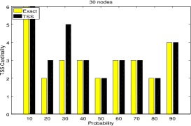
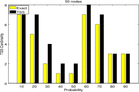
aaaaaaaaaaaaaaaaaaaaa (a) aaaaaaaaaaaaaaaaaaaaaaaaaaaaaaaaaa (b) aaaaaaaaaaaaaaaaaaaa

Figure 4: Experiments for random graphs $G(n,p)$ on $n$ nodes (any possible edge occurs independently with probability $0<p<1$). (a) $n=30$, (b) $n=50$ with $p\in\{10/100,20/100,\ldots,90/100\}$. For each node the threshold was fixed to a random value between 1 and the node degree.

5.2 Large Real-Life Networks

We performed experiments on several real social networks of various sizes from the Stanford Large Network Data set Collection (SNAP) [32] and the Social Computing Data Repository at Arizona State University [39]. The data sets we considered include both networks for which small target sets exist and networks needing larger target sets (due to the existence of communities, i.e., tightly connected disjoint groups of nodes that appear to delay the diffusion process).

Test Network

Experiments have been conducted on the following networks:

• BlogCatalog [39]: a friendship network crawled from BlogCatalog, a social blog directory website which manages the bloggers and their blogs. It has 88,784 nodes and 4,186,390 edges. Each node represents a blogger and the network contains an edge $(u,v)$ if blogger $u$ is friend of blogger $v$.

• BlogCatalog2 [39]: a friendship network crawled from BlogCatalog. It has 97,884 nodes and 2,043,701 edges.

• BlogCatalog3 [39]: a friendship network crawled from BlogCatalog. It has 10,312 nodes and 333,983 edges.

• BuzzNet [39]: BuzzNet is a photo, journal, and video-sharing social media network. It has 101,168 nodes and 4,284,534 edges.

• CA-AstroPh[32]: A collaboration network of Arxiv ASTRO-PH (Astro Physics). It has 18,772 nodes and 198,110 edges. Each node represents an author and the network contains an edge $(u,v)$ if an author $u$ co-authored a paper with author $v$.

• ca-CondMath [32] A collaboration network of Arxiv COND-MAT (Condense Matter Physics). It has 23,133 nodes and 93,497 edges.

• ca-GrQc [32]: A collaboration network of Arxiv GR-QC (General Relativity and Quantum Cosmology), It has 5,242 nodes and 14,496 edges.

• ca-HepPh [32]: A collaboration network of Arxiv HEP-PH (High Energy Physics - Phenomenology), it covers papers from January 1993 to April 2003. It has 10,008 nodes and 118,521 edges.

• ca-HepTh [32]: A collaboration network of HEP-TH (High Energy Physics - Theory) It has 9,877 nodes and 25,998 edges.

• Delicious [39]: A friendship network crawled on Delicious, a social bookmarking web service for storing, sharing, and discovering web bookmarks. It has 103,144 nodes and 1,419,519 edges.

• Douban [39]: A friendship network crawled on Douban.com, a Chinese website providing user review and recommendations for movies, books, and music. It has 154,907 nodes and 654,188 edges.

• Lastfm [39]: Last.fm is a music website, founded in UK in 2002. It has claimed over 40 million active users based in more than 190 countries. It has 108,493 nodes and 5,115,300 edges.

• Livemocha [39]: Livemocha is the world’s largest online language learning community, offering free and paid online language courses in 35 languages to more than 6 million members from over 200 countries around the world. It has 104,438 nodes and 2,196,188 edges.

• YouTube2 [32]: is a data set crawled from YouTube, the video-sharing web site that includes a social network. In the Youtube social network, users form friendship each other and users can create groups which other users can join. It contains 1,138,499 users and 2,990,443 edges.

The main characteristics of the studied networks are shown in Table 1. In particular, for each network we report the maximum degree, the diameter, the size of the largest connected component (LCC), the number of triangles, the clustering coefficient and the network modularity [33].

Name	Max deg	Diam	LCC size	Triangles	Clust Coeff	Modul.
BlogCatalog [39]	9444	–	88784	51193389	0.4578	0.3182
BlogCatalog2 [39]	27849	5	97884	40662527	0.6857	0.3282
BlogCatalog3 [39]	3992	5	10312	5608664	0.4756	0.2374
BuzzNet [39]	64289	–	101163	30919848	0.2508	0.3161
ca-AstroPh [32]	504	14	17903	1351441	0.6768	0.3072
ca-CondMath [32]	279	14	21363	173361	0.7058	0.5809
ca-GrQc [32]	81	17	4158	48260	0.6865	0.7433
ca-HepPh [32]	491	13	11204	3358499	0.6115	0.5085
ca-HepTh [32]	65	17	8638	28399	0.5994	0.6128
Delicious [32]	3216	–	536108	487972	0.0731	0.602
Douban [39]	287	9	154908	40612	0.048	0.5773
Last.fm [39]	5140	–	1191805	3946212	0.1378	0.1378
Livemocha [39]	2980	6	104103	336651	0.0582	0.36
Youtube2 [39]	28754	–	1134890	3056537	0.1723	0.6506

Table 1: Networks parameters.

The competing algorithms.

We compare the performance of our algorithm TSS toward that of the best, to our knowledge, computationally feasible algorithms in the literature. Namely, we compare to Algorithm TIP_DECOMP recently presented in [36], in which nodes minimizing the difference between degree and threshold are pruned from the graph until a “core” set is produced. We also compare our algorithm to the VirAds algorithm presented in [21]. Finally, we compare to an (enhanced) Greedy strategy (given in Figure 5), in which nodes of maximum degree are iteratively inserted in the target set and pruned from the graph. Nodes that remains with zero threshold are simply eliminated from the graph, until no node remains.

Algorithm GREEDY-TSS($G$)

Input: A graph $G=(V,E)$ with thresholds $t(v)$ for $v\in V$.

$S=\emptyset$

$U=V$

for each $v\in V$ do {

${\delta}(v)=d(v)$

$k(v)=t(v)$

$N(v)=\Gamma(v)$

}

while $U\neq\emptyset$ do {

$v={\tt argmin_{u\in U}\left\{k(u)\right\}}$

if $k(v)>0$ then {

$v={\tt argmax}_{u\in U}\left\{\delta(u)\right\}$

$S=S\cup\{v\}$

}

for each $u\in N(v)$ do     {

$k(u)=\max\{0,k(u)-1\}$

${\delta}(u)={\delta}(u)-1$

$N(u)=N(u)-\{v\}$

$U=U-\{v\}$

}

}

Figure 5: GREEDY-TSS($G$)

Thresholds values.

According to the scenario considered in [36], in our experiments the thresholds are constant among all vertices (precisely the constant value is an integer in the interval $[1,10]$ and for each vertex $v$ the threshold $t(v)$ is set as $min\{t,d(v)\}$ where $t=1,2,\ldots,10$.

Results.

Figures 6–19 depict the experimental results on large real-life networks. For each network the results are reported in a separated plot. For each plot the value of the threshold parameter appears along the X-axis, while the size of the solution appears along the Y-axis. For each dataset, we compare the performance of our algorithm TSS to the algorithm TIP_DECOMP [36], to the algorithm VirAds [21], and to the Greedy strategy.

All test results consistently show that the TSS algorithm we introduce in this paper presents the best performances on all the considered networks, while none among TIP_DECOMP, VirAds, and Greedy is always better than the other two.

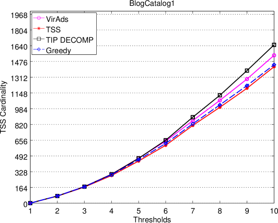
Figure 6: BlogCatalog [39].

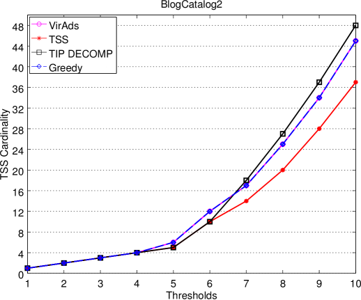
Figure 7: BlogCatalog2 [39].

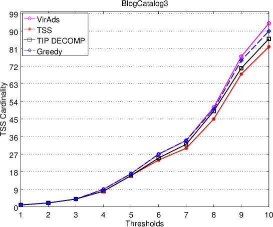
Figure 8: BlogCatalog3 [39].

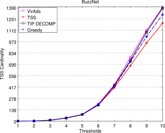
Figure 9: BuzzNet [39].

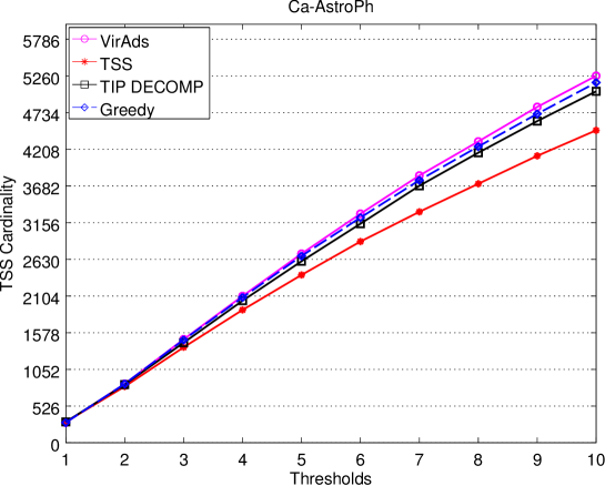
Figure 10: CA-Astro-Ph[32].

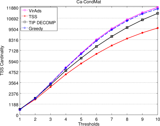
Figure 11: Ca-CondMat [32].

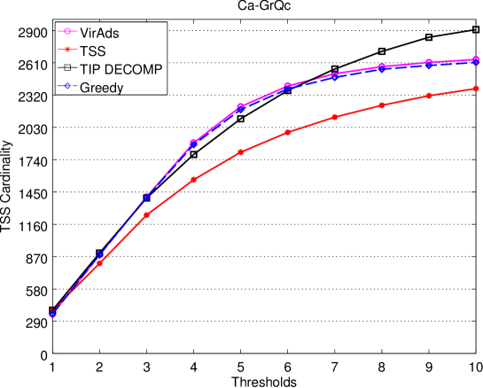
Figure 12: CA-GR-QC [32].

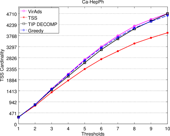
Figure 13: CA-HepPh [32].

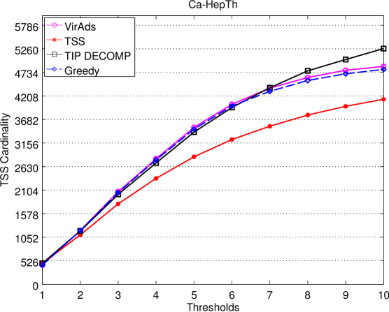
Figure 14: Ca-HepTh [32].

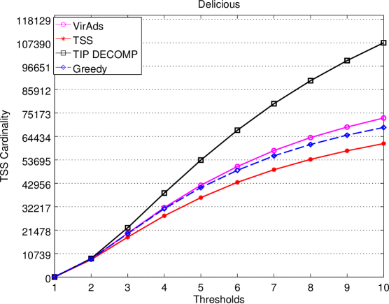
Figure 15: Delicious [39].

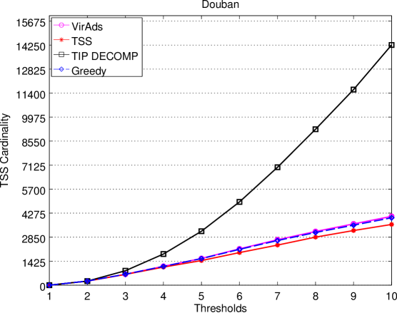
Figure 16: Douban [39].

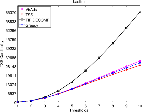
Figure 17: Lastfm [39].

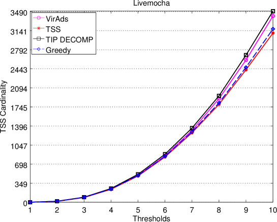
Figure 18: Livemocha [39].

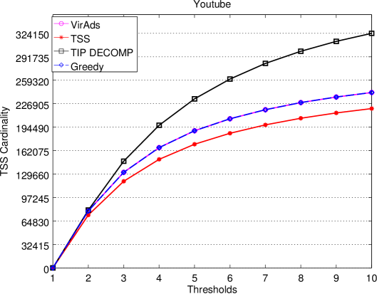
Figure 19: YouTube2 [32].

6 Concluding Remarks

We presented a simple algorithm to find small sets of nodes that influence a whole network, where the dynamic that governs the spread of influence in the network is given in Definition 1. In spite of its simplicity, our algorithm is optimal for several classes of graphs, it improves on the general upper bound given in [1] on the cardinality of a minimal influencing set, and outperforms, on real life networks, the performances of known heuristics for the same problem. There are many possible ways of extending our work. We would be especially interested in discovering additional interesting classes of graphs for which our algorithm is optimal (we conjecture that this is indeed the case).

References

- [1] Eyal Ackerman, Oren Ben-Zwi, and Guy Wolfovitz. Combinatorial model and bounds for target set selection. Theoretical Computer Science, 411(44–46):4017–4022, 2010.
- [2] Cristina Bazgan, Morgan Chopin, André Nichterlein, and Florian Sikora. Parameterized approximability of maximizing the spread of influence in networks. Journal of Discrete Algorithms, 27:54–65, 2014.
- [3] Oren Ben-Zwi, Danny Hermelin, Daniel Lokshtanov, and Ilan Newman. Treewidth governs the complexity of target set selection. Discrete Optimization, 8(1):87–96, 2011.
- [4] Robert M. Bond, Christopher J. Fariss, Jason J. Jones, Adam D. I. Kramer, Cameron Marlow, Jaime E. Settle, and James H. Fowler. A 61-million-person experiment in social influence and political mobilization. Nature, 489:295–298, 2012.
- [5] Carmen C. Centeno, Mitre C. Dourado, Lucia Draque Penso, Dieter Rautenbach, and Jayme L. Szwarcfiter. Irreversible conversion of graphs. Theoretical Computer Science, 412(29):3693–3700, 2011.
- [6] Ning Chen. On the approximability of influence in social networks. SIAM Journal on Discrete Mathematics, 23(3):1400–1415, 2009.
- [7] Wei Chen, Carlos Castillo, and Laks Lakshmanan. Information and Influence Propagation in Social Networks. Morgan & Claypool, 2013.
- [8] Chun-Ying Chiang, Liang-Hao Huang, Bo-Jr Li, Jiaojiao Wu, and Hong-Gwa Yeh. Some results on the target set selection problem. Journal of Combinatorial Optimization, 25(4):702–715, 2013.
- [9] Chun-Ying Chiang, Liang-Hao Huang, and Hong-Gwa Yeh. Target set selection problem for honeycomb networks. SIAM Journal on Discrete Mathematics, 27(1):310–328, 2013.
- [10] Morgan Chopin, André Nichterlein, Rolf Niedermeier, and Mathias Weller. Constant thresholds can make target set selection tractable. Theory of Computing Systems, 55(1):61–83, 2014.
- [11] Nicholas A. Christakis and James H. Fowler. Connected: The Surprising Power of Our Social Networks and How They Shape Our Lives – How Your Friends’ Friends’ Friends Affect Everything You Feel, Think, and Do. Back Bay Books, reprint edition, January 2011.
- [12] Ferdinando Cicalese, Gennaro Cordasco, Luisa Gargano, Martin Milanič, Joseph Peters, and Ugo Vaccaro. Spread of influence in weighted networks under time and budget constraints. Theoretical Computer Science, 586:40–58, 2015.
- [13] Ferdinando Cicalese, Gennaro Cordasco, Luisa Gargano, Martin Milanič, and Ugo Vaccaro. Latency-bounded target set selection in social networks. Theoretical Computer Science, 535:1 – 15, 2014.
- [14] Amin Coja-Oghlan, Uriel Feige, Michael Krivelevich, and Daniel Reichman. Contagious sets in expanders. In Proceedings of the Twenty-Sixth Annual ACM-SIAM Symposium on Discrete Algorithms, pages 1953–1987, 2015.
- [15] G. Cordasco, L. Gargano, and A. A. Rescigno. On finding small sets that influence large networks. Social Network Analysis and Mining (SNAM), 2016.
- [16] Gennaro Cordasco, Luisa Gargano, Marco Mecchia, Adele A. Rescigno, and Ugo Vaccaro. A fast and effective heuristic for discovering small target sets in social networks. In Proc. of COCOA 2015, volume 9486, pages 193–208, 2015.
- [17] Gennaro Cordasco, Luisa Gargano, Adele A. Rescigno, and Ugo Vaccaro. Optimizing Spread of Influence in Social Networks via Partial Incentives. In Structural Information and Communication Complexity: 22nd International Colloquium, SIROCCO 2015, pages 119–134. Springer International Publishing, 2015.
- [18] Gennaro Cordasco, Luisa Gargano, Adele A. Rescigno, and Ugo Vaccaro. Brief announcement: Active information spread in networks. In Proceedings of the 2016 ACM Symposium on Principles of Distributed Computing, PODC ’16, pages 435–437, New York, NY, USA, 2016. ACM.
- [19] Gennaro Cordasco, Luisa Gargano, Adele A. Rescigno, and Ugo Vaccaro. Evangelism in social networks. In Combinatorial Algorithms - 27th International Workshop, IWOCA 2016, Helsinki, Finland, August 17-19, 2016, Proceedings, pages 96–108, 2016.
- [20] Gennaro Cordasco, Luisa Gargano, and Adele Anna Rescigno. Influence propagation over large scale social networks. In Proceedings of the 2015 IEEE/ACM International Conference on Advances in Social Networks Analysis and Mining, ASONAM 2015, Paris, France, pages 1531–1538, 2015.
- [21] Thang N. Dinh, Huiyuan Zhang, Dzung T. Nguyen, and My T. Thai. Cost-effective viral marketing for time-critical campaigns in large-scale social networks. IEEE/ACM Trans. Netw., 22(6):2001–2011, December 2014.
- [22] Pedro Domingos and Matt Richardson. Mining the network value of customers. In Proceedings of the Seventh ACM SIGKDD International Conference on Knowledge Discovery and Data Mining, KDD ’01, pages 57–66, New York, NY, USA, 2001.
- [23] David Easley and Jon Kleinberg. Networks, Crowds, and Markets: Reasoning About a Highly Connected World. Cambridge University Press, New York, NY, USA, 2010.
- [24] Luisa Gargano, Pavol Hell, Joseph G. Peters, and Ugo Vaccaro. Influence diffusion in social networks under time window constraints. Theor. Comput. Sci., 584(C):53–66, 2015.
- [25] Luisa Gargano and Adele A. Rescigno. Complexity of conflict-free colorings of graphs. Theoretical Computer Science, 566:39 – 49, 2015.
- [26] Mark Granovetter. Threshold models of collective behavior. The American Journal of Sociology, 83(6):1420–1443, 1978.
- [27] David Kempe, Jon Kleinberg, and Éva Tardos. Maximizing the spread of influence through a social network. In Proceedings of the Ninth ACM SIGKDD International Conference on Knowledge Discovery and Data Mining, KDD ’03, pages 137–146, New York, NY, USA, 2003.
- [28] David Kempe, Jon Kleinberg, and Éva Tardos. Influential nodes in a diffusion model for social networks. In Proceedings of the 32Nd International Conference on Automata, Languages and Programming, ICALP’05, pages 1127–1138, Berlin, Heidelberg, 2005.
- [29] D. Lately. An army of eyeballs: The rise of the advertisee. The Baffler, Sep 2014.
- [30] Matti Leppaniemi, Heikki Karjaluoto, Heikki Lehto, and Anni Goman. Targeting young voters in a political campaign: Empirical insights into an interactive digital marketing campaign in the 2007 finnish general election. Journal of Nonprofit & Public Sector Marketing, 22(1):14–37, 2010.
- [31] Jure Leskovec, Lada A. Adamic, and Bernardo A. Huberman. The dynamics of viral marketing. ACM Trans. Web, 1(1), May 2007.
- [32] Jure Leskovec and Andrej Krevl. SNAP Datasets: Stanford large network dataset collection. http://snap.stanford.edu/data, 2015.
- [33] Mark E. J. Newman. Modularity and community structure in networks. Proceedings of the National Academy of Sciences of the United States of America (PNAS), 103(23):8577–8582, 2006.
- [34] André Nichterlein, Rolf Niedermeier, Johannes Uhlmann, and Mathias Weller. On tractable cases of target set selection. Social Network Analysis and Mining, 3(2):233–256, 2013.
- [35] T. V. Thirumala Reddy and C. Pandu Rangan. Variants of spreading messages. J. Graph Algorithms Appl., 15(5):683–699, 2011.
- [36] Paulo Shakarian, Sean Eyre, and Damon Paulo. A scalable heuristic for viral marketing under the tipping model. Social Network Analysis and Mining, 3(4):1225–1248, 2013.
- [37] K. Tumulty. Obama’s viral marketing campaign. TIME Magazine, July 2007.
- [38] Stanley Wasserman and Katherine Faust. Social Network analysis: Methods and Applications. Cambridge University Press, 1994.
- [39] Reza Zafarani and Huan Liu. Social computing data repository at ASU. http://socialcomputing.asu.edu, 2009.
- [40] Manouchehr Zaker. On dynamic monopolies of graphs with general thresholds. Discrete Mathematics, 312(6):1136–1143, 2012.