Visualizing electromagnetic vacuum by MRI

SUPPORTING INFORMATION
for
Visualizing electromagnetic vacuum by MRI

Abstract

Based upon Maxwell’s equations, it has long been established that oscillating electromagnetic (EM) fields incident upon a metal surface decay exponentially inside the conductor [1, 2, 3], leading to a virtual EM vacuum at sufficient depths. Magnetic resonance imaging (MRI) utilizes radiofrequency (r.f.) EM fields to produce images. Here we present the first visualization of a virtual EM vacuum inside a bulk metal strip by MRI, amongst several novel findings.

We uncover unexpected MRI intensity patterns arising from two orthogonal pairs of faces of a metal strip, and derive formulae for their intensity ratios, revealing differing effective elemental volumes (voxels) underneath these faces.

Further, we furnish chemical shift imaging (CSI) results that discriminate different faces (surfaces) of a metal block according to their distinct nuclear magnetic resonance (NMR) chemical shifts, which holds much promise for monitoring surface chemical reactions noninvasively.

Bulk metals are ubiquitous, and MRI is a premier noninvasive diagnostic tool. Combining the two, the emerging field of bulk metal MRI can be expected to grow in importance. The fundamental nature of results presented here may impact bulk metal MRI and CSI across many fields.

1 Introduction

MRI is a household name as a diagnostic tool in the medical field [10, 11], with an impressive resume in many other fields, including the study of materials [12, 13, 14, 15], corrosion of metals, monitoring batteries and supercapacitors [16, 17].

However, historically, MRI of bulk metals has been very rare, limited to specialized cells using r.f. gradients (with limited control) [18], instead of the magnetic field gradients employed in conventional MRI. In other studies involving bulk metals, the MRI targeted the surrounding dielectric (electrolyte in electrochemical and fuel cells with metallic electrodes, or tissues with embedded metallic implants) [19, 20, 21, 22, 23, 24, 25, 26, 27, 28, 29, 30]. Notwithstanding, these studies addressed issues that can cause distortions and limit sensitivity of the MRI images, such as bulk magnetic susceptibility (BMS) effects and eddy currents (produced on bulk metal surface due to gradient switching).

The dearth of mainstream bulk metal MRI is rooted in unique challenges posed by the physics of propagation of r.f. EM fields in bulk metals (MRI employs r.f. pulses to generate the MR signal leading to the images). All along, it has been known that the incident r.f. field decays rapidly and exponentially inside the metallic conductor (Fig.1), a phenomenon known as skin effect [1, 2, 3]. The characteristic length of decay ($\delta$, the skin depth), typically of the order of several microns (Eq.(S13)), characterizes the limited r.f. penetration into the metal. This in turn, results in attenuated MR signal intensity for bulk metals [19, 4]. Turning the tables, Bhattacharyya et. al.,[4] exploited the skin effect to separate and quantify bulk and non-bulk metal NMR signals in Li ion batteries to monitor the growth of dendritic metallic structures. Subsequently, for bulk metal MRI, yet another impediment was correctly diagnosed [5]. It was found that the orientation of the bulk metal surface, relative to $\bf B_{1}$(the r.f. magnetic field), critically affected the outcome. Using optimal alignment of the bulk metal (electrodes), relative to $\bf B_{1}$, recent studies have successfully demonstrated and highlighted bulk metal MRI albeit, primarily applied to batteries and electrochemical cells [5, 6, 7, 8, 9].

Though unanticipated at the time, the recent bulk metal MRI findings eased the implementation of MRI of liquid electrolyte, by helping mitigate adverse effects due to the metal in the vicinity of lithium, zinc and titanium electrodes, yielding fresh insights [7, 8, 31, 32, 33]. Similar benefits may be expected to accrue for MRI based radiology of soft tissues with embedded metallic implants (pacemeakers, prosthetics, dental implants, etc.).

Here, we present several key findings on bulk metal MRI and CSI:

• During a systematic noninvasive thickness measurement of bulk metal strips by MRI [7] (section SS8), we come across unexpected regions of intensity, and assign them to two mutually orthogonal pairs of faces of the strip.

• To explain the peculiar ratios of intensities from these different regions in bulk metal MRI and CSI, we derive formulae from first principles, unveling a surprising underlying reason: differing effective elemental volumes for these different regions.

• In the process, the images enable a visualization of a virtual EM vacuum inside the bulk metal via an MRI tunnel.

• Additionally, we demonstrate that the bulk metal CSI distinguishes different faces (surfaces) of a metal block according to their distinct NMR chemical shifts.

We attained these by employing three phantoms (samples) P0, P1, P3, depicted schematically in Fig.S1 and described in Methods section 6.1. All phantoms were derived from the same stock of 0.75 $mm$ thick lithium (Li) strip. Phantom P3 is a super strip composed of three Li strips pressed together, forming an effective single strip three times thicker than the individual strips in phantoms P0 and P1.

The setup of phantoms, r.f. coil and the gradient assembly ensures that the imaging directions $x,y,z$ fulfill the condition that $x\parallel a\parallel\mbox{$\bf B_{1}$}$ and $z\parallel\mbox{$\bf B_{0}$}$ (the static main magnetic field), with the possibility to reorient the phantom about the $x$-axis; $a,b,c$ are the three sides of the strips.

Since all MRI and CSI images to follow were acquired with the given phantom’s $bc$ faces normal ($\perp$, perpendicular) to $\bf B_{1}$, these images bear the imprint of having no contribution from these faces to the magnetic resonance (MR) signal [5, 6, 7, 8], since $\bf B_{1}$ penetration into the metal is maximal when it is parallel ($\parallel$) to the metal surface, and minimal when $\perp$ metal surface [1, 5, 6].

For details on the MRI experiments, including the nomenclature, the reader is referred to Methods section 6.2.

2 MRI

Fig.2 furnishes stackplots (intensity along the vertical axis) of ⁷Li 2d MRI (without slice selection) of phantom P3. Panel (a) displays MRI($xy$). Panel (b) displays MRI($yz$).

It is straightforward to infer that the walls of high intensity regions in either image emanate from $ac$ faces of the P3 strip [5, 6, 7], as we did while measuring the thickness of metal strips (Figs.S2 and S3, section SS8). In either image, contributions along the non imaged axis sum up to yield the high intensity walls.

However, the unexpected intensity between the two $ac$ faces of the super strip, in both the images, is perplexing. The 2d MRI($xy$) in Fig.2a exhibits a low intensity plateau spanning the walls. The 2d MRI($yz$) in Fig.2b displays low intensity ridges bridging the walls.

2.1 Visualizing a virtual eletromagnetic vacuum by MRI

To understand better these unexpected regions of intensity, we acquired ⁷Li 3d MRI($xyz$) of phantom P3, shown in Fig.3. In addition to the $ac$ faces (separated along $y$), the $ab$ faces (separated along $z$) are revealed for the first time.

As noted earlier, $bc$ faces (being $\perp$ to $\bf B_{1}$) are absent. The hollow region in MRI($xyz$) arises from the skin depth phenomenon [4, 5, 6, 1, 2, 3], restricting the EM fields to effectively access only a limited subsurface underneath the $ac$ and $ab$ faces (section SS7 and Fig.1). The presence of faces $\parallel$ $\bf B_{1}$, coupled with the conspicuous absence of faces $\perp$ $\bf B_{1}$, in combination with the hollow region, imparts the 3d image an appearance of an MRI tunnel, supplying a compelling visualization of a virtual EM vacuum in the interior of a metallic conductor (hitherto depicted only schematically in literature (for e.g. Ref.[4])).

With the aid of 3d MRI in Fig.3, the intensity regions in 2d MRI($xy$) and 2d MRI($yz$) images of Fig.2, can be easily interpreted as simply regions resulting respectively from projections along $z$ and $x$ axes of the 3d image. It is convincingly clear that the intensity between $ac$ faces (either the plateau or the ridges), is due to the pair of $ab$ faces of the superstrip P3.

Yet, the basis for the relative intensity values remains elusive at this stage.

For the 2d MRI($xy$) in Fig.2a, it can be argued that, for the $ac$ face the entire length of side $c=$7 $mm$ (Fig.S1) contributes to the signal, while for the $ab$ face, only a subsurface depth $\mbox{$\delta_{\text{eff}}$}\approx$ 9.49 $\mu m$ contributes (Eq.(S13), Eq.(S18), section SS7 and Fig.1). This would lead to a ratio of the corresponding intensities, $S_{ac}/S_{ab}$, to be of the order of $c/(2\mbox{$\delta_{\text{eff}}$})\approx 368$ (Fig.4a), in obvious and jarring disagreement with the observed ratio (of maxima of $S_{ac}$ and $S_{ab}$) of 6.6.

For the 2d MRI($yz$) in Fig.2b, the expected intensity pattern in a stack plot would be one with equal intensities from $ab$ and $ac$ faces, since they share the same side, $a$, along $x$ (non imaged) axis (Fig.4b). This again, is in stark contrast with the observed ratio (of maxima of $S_{ac}$ and $S_{ab}$) of 10.

For the MRI($xyz$), naively, uniform intensity would be expected from both $ab$ and $ac$ faces, resulting in a ratio of unity. Instead, the observed ratio (of maxima of $S_{ac}$ and $S_{ab}$) is found to be 3.8.

Thus, the MRI images bear peculiar intensity ratios from comfortably identified (from 3d MRI) regions of the bulk metal. We will return to this topic later.

3 CSI

The ⁷Li NMR spectrum of phantom P3 (Fig.5 inset) contains two distinct peaks in the Knight shift region for metallic ⁷Li (see Methods section 6.2), centered at $\delta_{1}$= 256.4 and $\delta_{2}$= 266.3 ppm. At first sight it might seem odd that a metallic strip, of regular geometry and uniform density, that is entirely composed of identical Li atoms, gives rise to two NMR peaks instead of the expected single peak.

To gain additional insight as to the spatial distribution of the Li metal species with different NMR shifts, we turn to CSI, which combines an NMR chemical shift (CS) dimension with one or more imaging(I) dimensions [12, 34, 35, 36].

The 2d CSI($y$) shown in Fig.S4 comprises of two bands separated along $y$ located at $\delta_{2}$, along the CS dimension, while a low intensity band spans them along $y$ at a CS of $\delta_{1}$, strongly hinting at, the two bands (at $\delta_{2}$) being associated with $ac$ faces.

This observation called for adding an additional imaging dimension along $z$, leading to 3d CSI($yz$), which is realized in Fig.5, where $y$ and $z$ are the imaging dimensions, accompanied by the CS dimension. The bands separated along $z$, occur at $\delta_{1}$. The bands separated along $y$, occur at $\delta_{2}$. In conjunction with the 3d MRI image in Fig.3, it is evident that the pairs of bands at $\delta_{1}$ and $\delta_{2}$ arise from $ab$ and $ac$ faces respectively, completing the spatio-chemical assignment.

These assignments readily carry over to 2d CSI($y$) in Fig.S4, with the pair of bands at $\delta_{2}$ and the low ridge spanning them at $\delta_{1}$, being respectively identified with $ac$ and $ab$ faces. Similarly, in the NMR spectrum, the short and tall peaks respectively at $\delta_{1,2}$ are assigned to $ab$ and $ac$ faces, consistent with the reported [4, 6] experiments and simulations.

That different types of faces of the bulk metal strip suffer different NMR (Knight) shifts according to their orientations relative to $\bf B_{0}$, is consistent with previous observations and simulations [4, 6], and has been traced to bulk magnetic susceptibility (BMS) effect [4, 5, 6, 9, 37, 38, 39].

Interestingly, the 3d CSI sheds new light on previous bulk metal NMR studies. For instance, in an earlier study [4], a similar shift difference between NMR peaks was observed at $\parallel$ and $\perp$ orientations (relative to $\bf B_{0}$) of the major faces of a thinner metal strip, by carrying out two separate experiments. Here, phantom P3 furnishes these two orientations in a single experiment, via $ac$ and $ab$ faces (Fig.S1). The present work provides physical insight into another previous [6] observation. It was found that the intensity of NMR peak arising from $ab$ faces, unlike that from the $ac$ faces, was invariant under rotation about $z\parallel c\parallel B_{0}$ axis. Our 3d MRI (Fig.3) and 3d CSI (Fig.5), directly demonstrate that such a rotation leaves the orientation of $\bf B_{1}$ relative to $ab$ face (but not the $ac$ face) the same (signal intensity from a given face depends on its orientation relative to $\bf B_{1}$[5, 6]). Note that the shifts themselves remain unshifted since they depend on the orientation of the faces relative to $\bf B_{0}$, which does not change under this rotation ($ac$ and $bc$ faces remain $\parallel\mbox{$\bf B_{0}$}$, whilst $ab$ faces remain $\perp\mbox{$\bf B_{0}$}$).

Thus, bulk metal CSI supplies direct evidence, that the bulk metal chemical (Knight) shifts resulting from BMS are correlated with the differing orientations (relative to $\bf B_{0}$) of different parts of the bulk metal.

Like for MRI, the basis for the ratio of intensities from the $ac$ and $ab$ faces ($S_{ac}/S_{ab}\approx$ 2.8), is not immediately intuitively obvious and will be explored next.

4 Intensity ratio formulae for bulk metal MRI and CSI

The peculiar intensity ratios in MRI and CSI, of signals $S_{ab}$ and $S_{ac}$, arising respectively from $ab$ and $ac$ faces of phantom P3 (Fig.2, sections 2 and 3), could be due to gradient switching involved in the MRI experiments (the resultant eddy currents could be different for $ab$ and $ac$ faces). However, as shown in section SS9, this can be ruled out on the basis of 2d MRI($yz$) and MRI($zy$) at mutually orthogonal orientations (related by a rotation about $x\parallel a\parallel\mbox{$\bf B_{1}$}$), shown in Fig.S5.

And yet, it is possible to derive, from elementary considerations and first principles, and arrive at expressions for the ratios of MRI and CSI intensities from $ab$ and $ac$ faces.

For the 2d MRI($xy$), in Fig.2a, the signal intensity from the $ab$ faces can be written as (see Eq.(S19))

$$S_{ab}(x,y)\propto dx\ dy\ \int dz=dx\ dy\ 2\delta_{\text{eff}}$$ (1)

with $dx\ dy\ dz$ denoting elemental volume of the metal, and $\delta_{\text{eff}}$ is the effective subsurface depth that would account for the MR signal in the absence of $\bf B_{1}$ decay (see Eq.(S18) and Fig.1). Above, the integral over $z$, is replaced by $\delta_{\text{eff}}$  underneath the two $ab$ faces separated along $z$.

Similarly, for the signal intensity from either of the $ac$ faces,

$$S_{ac}(x,y)\propto dx\ dy\ \int dz=dx\ \delta_{\text{eff}}\ c$$ (2)

since the subsurface now is $\perp y$.

Eq.(1) and Eq.(2), reveal differing effective elemental volumes(voxels) underneath these faces:

$$dV_{\text{eff}}^{\text{ab}}=dx\ dy\ \delta_{\text{eff}}$$ (3)

$$dV_{\text{eff}}^{\text{ac}}=dx\ \delta_{\text{eff}}\ dz$$ (4)

From Eq.(1) and Eq.(2),

$$\frac{S_{ac}}{S_{ab}}=\frac{c}{2\Delta y}$$ (5)

where we have replaced $dy$ by $\Delta y$, the resolution along $y\ \parallel b$. Consulting the Methods section 6.2 and Fig.S1, $c=7$ $mm$, $\Delta y$=0.25 $mm$ and Eq.(5) yields a calculated ratio of $S_{ac}/S_{ab}$= 14 (as illustrated in Fig.6a), within an order of magnitude of the observed ratio (section 2, Fig.2a) and a 25 fold improvement relative to the expected ratio (Fig.4a).

Also, Eq.(5) reveals that $S_{ac}/S_{ab}$ increases with increasing resolution along $y$, as shown in the three images in Fig.S6, with relative resolutions increasing by factors of 1, 2 and 4, yielding calculated $S_{ac}/S_{ab}$ ratios of 7, 14 and 28 respectively. The corresponding observed ratios (of maxima of $S_{ac}$ and $S_{ab}$) of 3.3, 6.6, and 11.6, are within an order of magnitude of the calculated values. Remarkably, these observed ratios themselves increase by factors of 1, 2 and 3.5, mimicking closely the corresponding factors of resolution increase.

Continuing in the same vein, for the 2d MRI($yz$), in Fig.2b,

$$S_{ab}(y,z)\propto dy\ dz\int dx=a\ dy\ \delta_{\text{eff}}$$ (6)

while,

$$S_{ac}(y,z)\propto dy\ dz\int dx=a\ \delta_{\text{eff}}\ dz$$ (7)

leading to

$$\frac{S_{ac}}{S_{ab}}=\frac{\Delta z}{\Delta y}$$ (8)

once again, replacing $dy,\ dz$ by $\Delta y,\ \Delta z$, the respective resolutions along $y,\ z$. Using the values of $\Delta y,\Delta z$= 0.0357, 1 $mm$ in Eq.(8), ensues a calculated ratio of $S_{ac}/S_{ab}\approx$ 28 (as illustrated in Fig.6b), within an order of magnitude of the observed ratio (section 2, Fig.2b), and 3.5 fold better than the expected ratio (Fig.4b). More importantly, the expected intensity pattern is even qualitatively (visually) different from the experiment, unlike the derived pattern.

Similarly, for the 2d MRI($zy$) in Fig.S5b, of phantom P3 in horizontal orientation, it can be easily shown that,

$$\frac{S_{ac}}{S_{ab}}=\frac{\Delta y}{\Delta z}$$ (9)

Using the values of $\Delta z,\Delta y$= 0.0357, 1 $mm$ in Eq.(9), results in a calculated ratio of $S_{ac}/S_{ab}\approx$ 28, within an order of magnitude of the observed ratio (section SS9).

Proceeding along the same lines, for the MRI($xyz$) in Fig.3,

$$S_{ab}(x,y,z)\propto dx\ dy\ dz=dx\ dy\ \delta_{\text{eff}}$$ (10)

while,

$$S_{ac}(x,y,z)\propto dx\ dy\ dz=dx\ \delta_{\text{eff}}\ dz$$ (11)

As usual by now, replacing $dy,\ dz$ by $\Delta y,\ \Delta z$, the respective resolutions along $y,\ z$, we obtain again Eq.(8). Consulting the Methods section 6.2, $\Delta y,\Delta z$= 0.25, 1 $mm$, respectively. Using these values in Eq.(8) yields a calculated ratio of $S_{ac}/S_{ab}$= 4, within an order of magnitude of the observed ratio (section 2).

Fig.S7 shows (in stack plot representation, with vertical axis denoting intensity) $xy$ slices (along $z$) from the 3d MRI($xyz$). The central slice contains no signal between the walls of intensity (from $ac$ faces) as expected. However, the slice from the top $ab$ face exhibits a plateau of intensity between the $ac$ faces, visually demonstrating that $S_{ab}\neq S_{ac}$ in the non-hollow regions of the 3d image, in place of the expected uniform intensity.

Similarly, for the 3d CSI($yz$) in Fig.5, it can be shown that the ratio $S_{ac}/S_{ab}$ is given by Eq.(8), which along with the relevant experimental parameters for this image, yields a calculated value of 2, within an order of magnitude of the observed ratio (of maxima of $S_{ac}$ and $S_{ab}$) of 2.8.

On the other hand, for the 2d CSI($y$), in Fig.S4, it can be shown that the ratio $S_{ac}/S_{ab}$ is given by Eq.(5), from which we obtain a calculated value of 14, using the experimental parameters in section 6.2. The measured ratio (of maxima of $S_{ac}$ and $S_{ab}$) of 9.5, is again within an order of magnitude of the calculated value.

Thus, the $S_{ac}/S_{ab}$ ratios calculated from Eqs.(5), (8) and (9), agree with the observed values within an order of magnitude for 2d MRI($xy$), 2d MRI($yz$), 2d MRI($zy$), 3d MRI($xyz$), 3d CSI($yz$) and 2d CSI($y$). In fact, discrepancies between observed and derived $S_{ac}/S_{ab}$ ratios range only by factors of 0.7 to 2.8 across various MRI and CSI images (see Table.1). More importantly, the derived patterns resemble the observed patterns, unlike the expected patterns, which differ even visually from the observed patterns (for e.g., see Figs.2, 4 and 6).

Table 1: The observed, derived (from Eqs.(5), (8), (9)), and expected (from skin depth arguments alone) $S_{ac}/S_{ab}$ ratios.

		$S_{ac}/S_{ab}$
Experiment	Observed	Derived	Expected
MRI($xy$)
Fig.S6a	3.3	7	368
Fig.S6b	6.6	14	368
Fig.S6c	11.6	28	368
MRI($yz$)	10	28	1
MRI($zy$)	10	28	1
MRI($xyz$)	3.8	4	1
2d CSI($y$)	9.5	14	368
3d CSI($yz$)	2.8	2	1

In summary, the formulae unveil the underlying reason for the significant departure of observed $S_{ac}/S_{ab}$ from expected values: differing effective elemental volumes underneath these faces, as revealed by Eqs.(3) and (4). The derived patterns bear closer resemblance to experiment, than what is expected from skin depth consideratons alone, or from conventional specifications of the voxel= $\Delta x\Delta y\Delta z$ (see for e.g. Figs.2, 4 and 6).

On a practical note, these formulae can guide experimental strategies to relatively enhance MRI and CSI signals from different regions of the bulk metal.

5 Conclusions

In conclusion, the unexpected findings presented here may impact bulk metal MRI and CSI studies in general, via fresh insights for data collection, analysis and interpretation. The bulk metal MRI and CSI (correlating different bulk metal surfaces with distinct chemical shifts) results in this study have the noninvasive diagnostic potential in other fields such as structure of metals and alloys [40, 41], metallurgy (metal fatigue, fracture, strain) [42, 43, 44], catalysis [45, 46], bulk metal surface science and surface chemistry [47, 48, 49], metallic medical implants, dielectric MRI in the vicinity of bulk metals etc. (section 1).

The findings may also lead to as yet unforeseen applications (section 1) since, (i) they are of a fundamental nature, (ii) there are no inherent limitations to the approach employed (scalability, different metals, systems other than batteries, etc., are all possible), (iii) the study utilizes only standard MRI tools (hardware, pulse sequences, data acquisition and processing), ensuring ease of implementation and reproducibility. Thus it is likely to benefit from advances made in the mainstream (medical) MRI field.

6 Methods

6.1 Phantoms

All phantoms were assembled and sealed in an argon filled glove box. All three phantoms, P0, P1 and P3, shown in Fig.S1 (of dimensions $a\times b\times c$), were derived from a (0.75 $mm$ thick) stock Li strip (Alfa Aesar 99.9%). The Li strips were mounted on a 2.3 $mm$ thick teflon strip and the resulting sandwich bound together with Kapton tape. Each phantom was placed in a flat bottom glass tube (9.75 $mm$ inner diameter (I.D.), 11.5 $mm$ outer diameter (O.D.) and 5 $cm$ long), with the longest side, $a$, $\parallel$ to the tube axis and to the axis of the home built horizontal loop gap resonator (LGR) r.f. coil (32 $mm$ long, 15 $mm$ O.D.), thus guaranteeing $\mbox{$\bf B_{1}$}\parallel a$. The phantom containing glass tubes were wrapped with Scotch tape to snugly fit into the r.f. coil.

In Fig.S1, $x,y,z$ specify the imaging (gradient) directions, with $z\parallel\mbox{$\bf B_{0}$}$ (the main magnetic field). For our horizontal LGR r.f. coil (the MR resonator) and the gradient assembly system, $\mbox{$\bf B_{1}$}\parallel x$, resulting in $\mbox{$\bf B_{1}$}\parallel x\parallel a$.

• P0: Pair of Li strips separated by a teflon strip; for each Li strip, $a\times b\times c=$ 20 x 0.75 x 7 $mm^{3}$.

• P1: Single Li strip. $a\times b\times c=$ 15 x 0.75 x 7 $mm^{3}$.

• P3: Three Li strips pressed together to yield a single composite super strip. $a\times b\times c=$ 15 x 2.25 x 7 $mm^{3}$.

6.2 MRI and CSI

Magnetic resonance experiments were conducted on a $B_{0}$=21$T$ magnet (corresponding to ⁷Li Larmor frequency of 350 MHz) operating under Bruker Avance III system with Topspin spectrometer control and data acquisition, and equipped with a triple axes ($x,y,z$) gradient amplifier assembly, using a multinulcear MRI probe (for a triple axes 63 $mm$ I.D. gradient stack by Resonance Research Inc.), employing the LGR r.f. coil (resonating at 350 MHz) desribed above.

The MRI and CSI data were acquired using spin-echo imaging pulse sequence without slice selection [12, 34] (yielding sum total of signal conributions from the non imaged dimensions). Frequency encoding gradient was employed for the directly detected dimension and phase encoding gradients for the indirect dimensions [12, 34]. The CSI experiments were carried out with the NMR chemical shift as the directly detected dimension, with phase encoding gradients along the indirectly detected imaging dimensions. The r.f. pulses were applied at a carrier frequency of 261 ppm (to excite the metallic ⁷Li nuclear spins in the Knight shift region [4, 50]), typically with a strength of 12.5 $kHz$, with a recycle (relaxation) delay of 0.5 $s$. The gradient dephasing delay and phase encoding gradient duration were 0.5 $ms$.

Throughout this manuscript, the first axis label ($x,y,z$) describing an MRI experiment stands for frequency encoding dimension and the remaining ones correspond to phase econded dimensions. For e.g., MRI($xyz$) implies frequency encoding along $x$ axis, and phase encoding along the remaining directions.

$G_{x},G_{y},G_{z}$ and $N_{x},N_{y},N_{z}$ denote respectively the gradient strengths in units of $T/m$ and number of data points in $k$-space (^∗ denoting complex number of points acquired in quadrature) [12, 34], along $x,y,z$ axes. $L_{x},L_{y},L_{z}$ and $\Delta x,\Delta y,\Delta z$ are respectively the resultant nominal field of view (FOV) and resolution, in units of $mm$, along $x,y,z$ axes [12, 34].

Also, $n$ is the number of transients accumulated for signal averaging and $SW$ is the spectral width (in units of $kHz$) for the directly detected dimension in MRI and CSI.

1d MRI(y):
$n=64,\ SW=50$
$G_{y}=0.42,\ N_{y}^{*}=200,\ L_{y}=7.143,\ \Delta y=0.0357$
2d MRI(xy):
$n=32,\ SW=100$
$G_{x}=0.24,\ N_{x}^{*}=200,\ L_{x}=25,\ \Delta x=0.125$
$L_{y}=10$
(1) $G_{y}=0.12,\ N_{y}=20,\ \Delta y=0.500$ (Figs.S2a,S6a)
(2) $G_{y}=0.24,\ N_{y}=40,\ \Delta y=0.250$ (Figs.S2b,S3b,2a, S6b)
(3) $G_{y}=0.48,\ N_{y}=80,\ \Delta y=0.125$ (Fig.S6c)
2d MRI(yz):
$n=32$ $SW=50$
$G_{y}=0.42,\ N_{y}^{*}=200,\ L_{y}=7.143,\ \Delta y=0.0357$
$G_{z}=0.06,\ N_{z}=16,\ L_{z}=16,\ \Delta z=1.000$
2d MRI(zy):
$n=32,\ SW=50$
$G_{z}=0.42,\ N_{z}^{*}=200,\ L_{z}=7.143,\ \Delta z=0.0357$
$G_{y}=0.06,\ N_{y}=16,\ L_{y}=16,\ \Delta y=1.000$
MRI(xyz):
$n=16,\ SW=100$
$G_{x}=0.24,\ N_{x}^{*}=200,\ L_{x}=25,\ \Delta x=0.125$
$G_{y}=0.24,\ N_{y}=40,\ L_{y}=10,\ \Delta y=0.250$
$G_{z}=0.06,\ N_{z}=16,\ L_{z}=16,\ \Delta z=1.000$
2d CSI(y):
$n=8,\ SW=100$, number of data points(complex)=$1024$
$G_{y}=0.24,\ N_{y}=40,\ L_{y}=10,\ \Delta y=0.250$
3d CSI(yz):
$n=24,\ SW=100$, number of data points(complex)=$1024$
$G_{y}=0.12,\ N_{y}=20,\ L_{y}=10,\ \Delta y=0.500$
$G_{z}=0.06,\ N_{z}=16,\ L_{z}=16,\ \Delta z=1.000$

All data were processed in Bruker’s Topspin, with one zero fill prior to complex fast Fourier Transform (FFT) along each dimension either without any window function or with sine-bell window function. All data were ’normalized’ (to $\approx 10$, for plotting convenience) to aid comparing relative intensities from different regions within a given image. For the purpose of determining the ratios of signal intensities associated with different regions of the bulk metal, the intensity values were measured directly from the processed images either in Topspin or Matlab (for e.g., ’datatip’ utility in Matlab, yields the coordinates and the ’value’ (intensity) of a data point by clicking on it, in 1d, 2d and 3d plots).

AUTHOR CONTRIBUTIONS
CSC recognized and analyzed anomaly between observed and expected intensity patterns in the MRI and CSI images, prepared figures, analyzed data, interpreted and discussed results, helped write and proof read manuscript, carried out literature search.
AS prepared the phantoms, discussed results, helped write the manuscript.
EAT discussed results, helped write the manuscript.
DMT discussed results, helped write the manuscript.
SC conceptualized the project, designed phantoms, designed and conducted experiments, developed analytical tools, organized and analyzed data, interpreted results, derived intensity ratio equations, helped with figures, and wrote the manuscript.
All authors reviewed the manuscript.

Additional Information
Competing financial interests
The authors declare no competing financial interests.

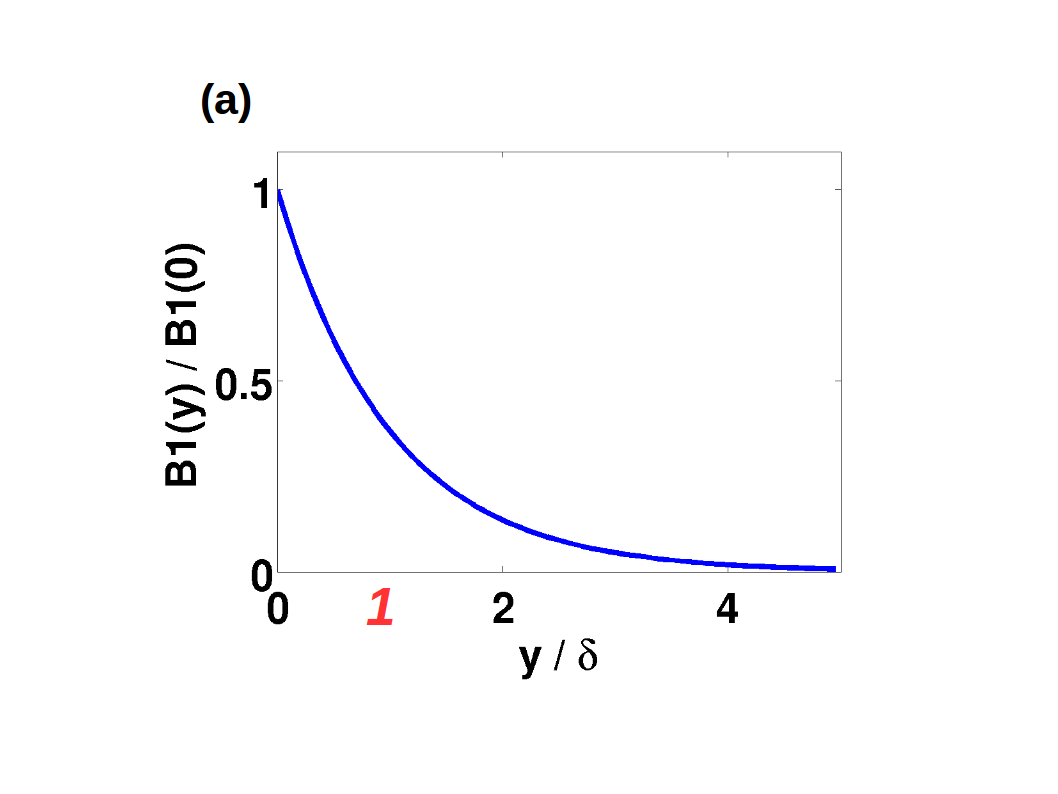
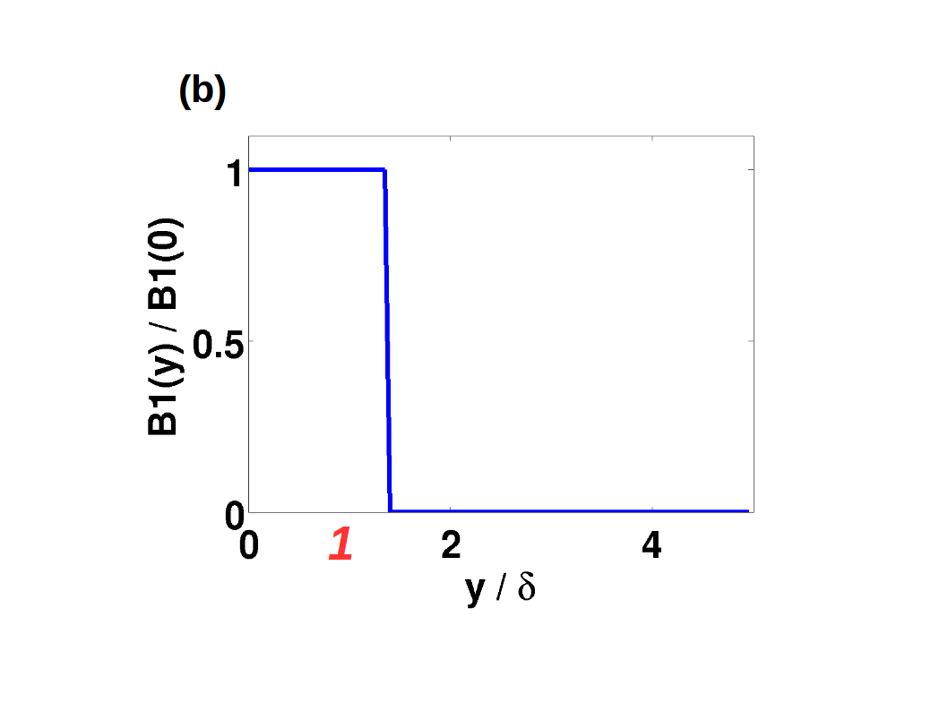
Figure 1: Skin depth $\delta$, and effective subsurface depth $\delta_{\text{eff}}$.
(a) Exponential decay of magnitude of $\bf B_{1}$($y$), as a function of the depth from the metal surface (see Eq.(S12) in section SS7).
(b) Effective subsurface depth $\delta_{\text{eff}}$, without $\bf B_{1}$decay, that would account for the MR signal (see Eq.(S18) in section SS7).

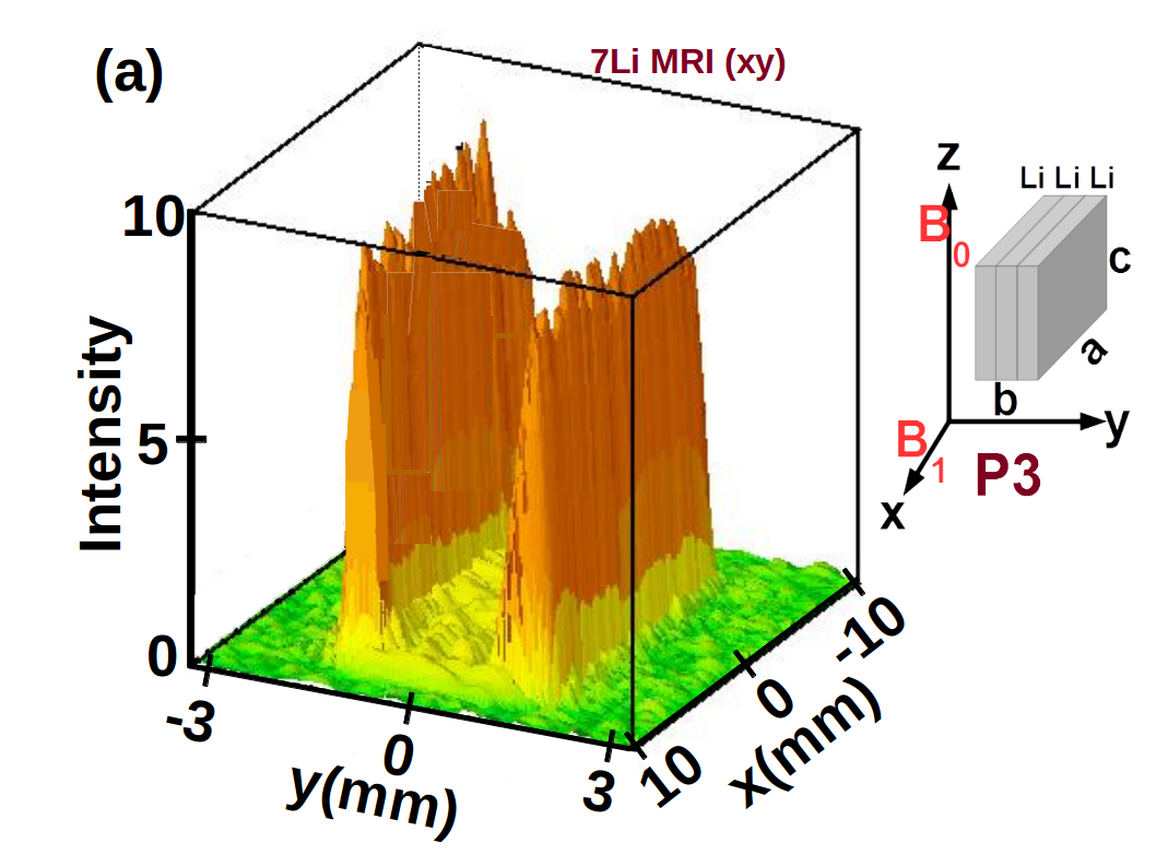
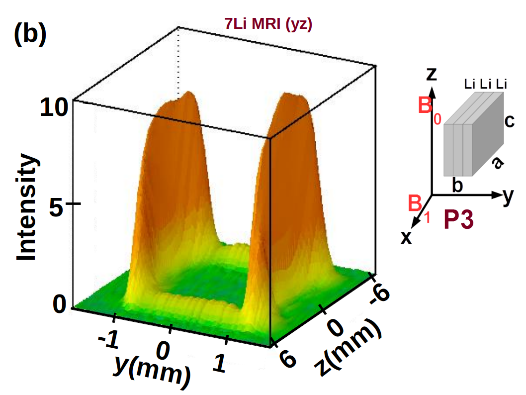
Figure 2: Surprising regions of intensity in bulk metal MRI.
⁷Li 2d MRI (sans slice selection) stack plots of phantom P3 (Fig.S1 and section 6). Vertical axis denotes intensity, resulting from the sum total of spin density along non imaged dimension.
(a) 2d MRI($xy$); same data as in blue, labeled P3, regions of Fig.S3b.
(b) 2d MRI($yz$).
In either image, there is no contribution from the $bc$ faces to the MR signal since they are $\perp$ $\bf B_{1}$(section 1).
In either image, the high intensity walls are easily associated with the $ac$ faces. (see Figs.S2, S3 and section SS8).
The intensity between the two $ac$ faces of the metal strip is evident in both images. Note the low intensity plateau and the ridges between the walls, respectively in the MRI($xy$) and MRI($yz$) images. Regarding these novel regions of intensity, see section 2. See also Fig. 4.

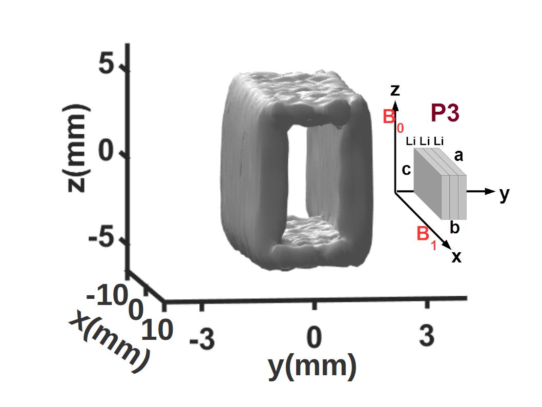
Figure 3: Peering at a virtual electromagnetic vacuum through an MRI tunnel.
⁷Li 3d MRI($xyz$) of phantom P3 (Fig.S1). In addition to the already identified $ac$ faces in previous images (Figs.2, S2 and S3), the $ab$ faces are revealed for the first time, accounting for the low intensity regions in Fig.2. The $bc$ faces are conspicuous by absence, being $\perp$ $\bf B_{1}$. The resulting MRI tunnel supplies a compelling visual of peering at a virtual EM vacuum in the interior of a metallic conductor (see section 2).

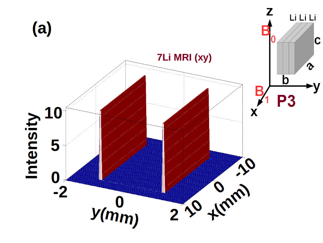
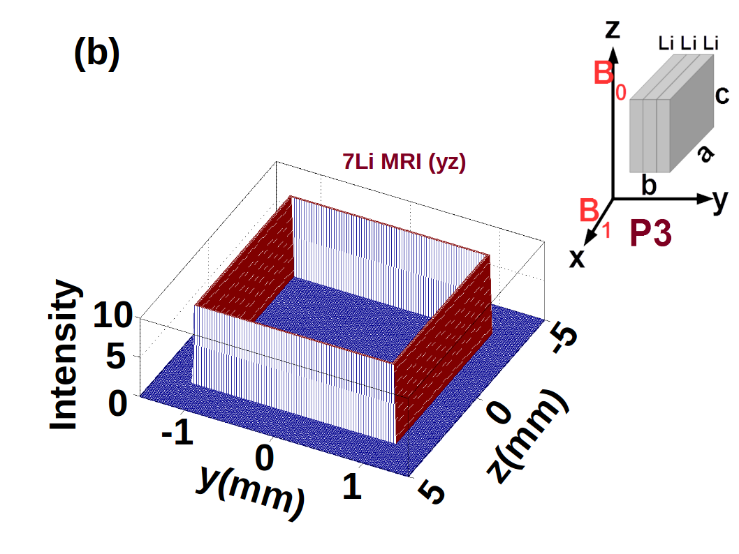
Figure 4: Expected relative intensities in bulk metal MRI.
Illustration of expected relative intensities from different pairs of faces in bulk metal ⁷Li 2d MRI of phantom P3 as stack plots (intensity along vertical axis): (a) 2d MRI($xy$). (b) 2d MRI($yz$).
In either illustration, there is no contribution from the $bc$ faces to the MR signal since they are $\perp$ $\bf B_{1}$(section 1).
For MRI($xy$) in panel (a), the expected ratio of signal intensities from $ac$ and $ab$ faces ($S_{ac}/S_{ab}\approx 368$) is in obvious disagreement with experiment (Fig.2a).
For MRI($yz$) in panel (b), one would naively expect that $S_{ac}=S_{ab}$, which again is in striking departure from the experiment (Fig.2b). See section 2.

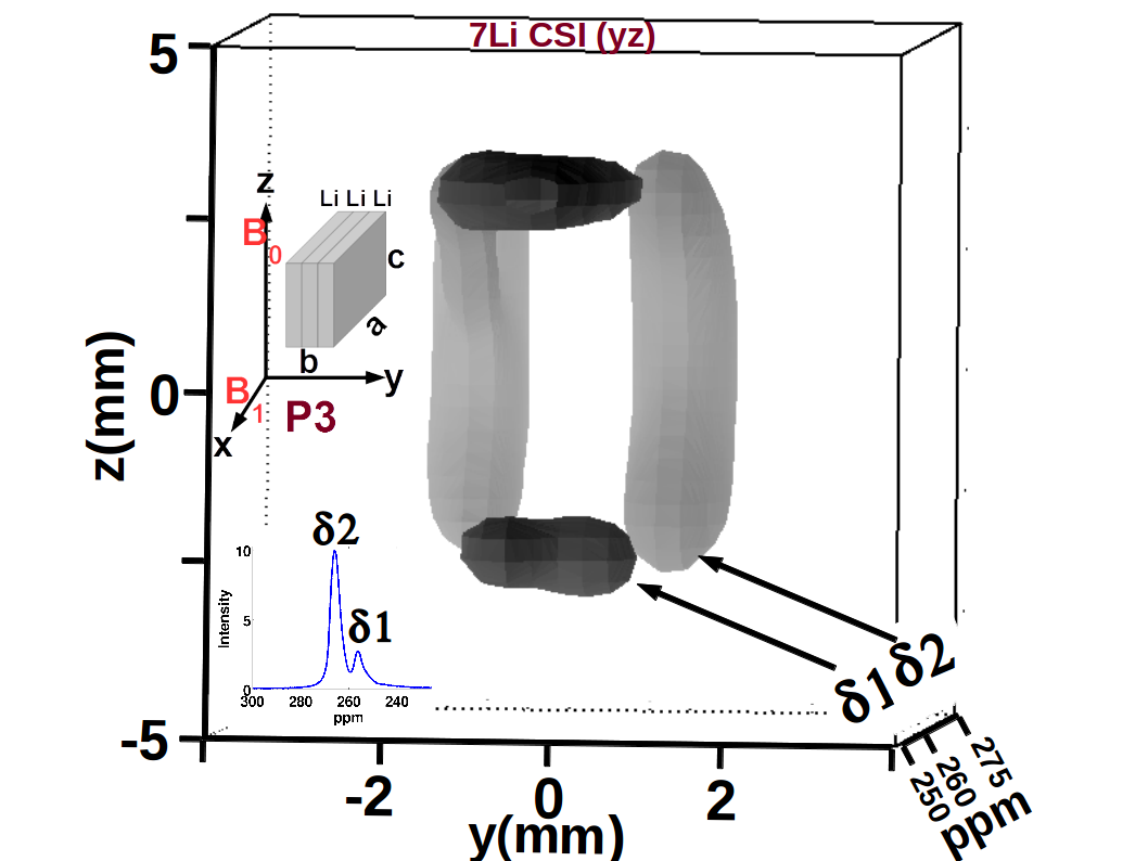
Figure 5: Chemical shift imaging of a bulk metal strip.
⁷Li 3d CSI($yz$) of phantom P3: chemical shift, $y$ and $z$ axes comprise the three dimensions.
Despite being composed of identical Li atoms, ⁷Li NMR spectrum (inset) of phantom P3 exhibits two peaks, instead of the expected single peak (section 3). Short and tall peaks are centered respectively at $\delta_{1}$= 256.4 and $\delta_{2}$= 266.3 ppm.
In the CSI, bands separated along $z$, occur at CS $\delta_{1}$. The bands separated along $y$, occur at CS $\delta_{2}$.
In conjunction with the 3d MRI (Fig.3) and P3 schematics (Fig.S1), the pair of bands at $\delta_{1}$ are assigned to $ab$ faces, and pair of bands at $\delta_{2}$ are assigned to $ac$ faces (thus completing the assignment of both the 2d CSI($y$) in Fig.S4, and the NMR spectrum itself).

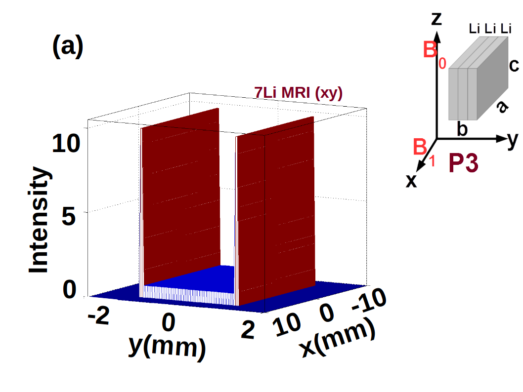
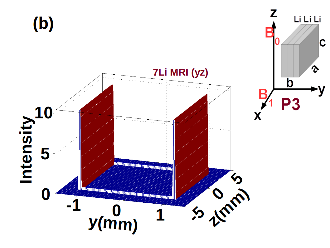
Figure 6: Predicted relative intensities in bulk metal MRI.
Illustration of predicted (from the derived formulae) relative intensities from different pairs of faces in bulk metal ⁷Li 2d MRI of phantom P3 as stack plots (intensity along vertical axis).
(a) 2d MRI($xy$) based on Eq.(5): $S_{ac}/S_{ab}=14$.
(b) 2d MRI($yz$) based on Eq.(8): $S_{ac}/S_{ab}=28$.
In either illustration, there is no contribution from the $bc$ faces to the MR signal since they are $\perp$ $\bf B_{1}$(section 1).
Compare and contrast with the corresponding experimental images in Fig.2, and the illustration of expected images in Fig.4. See sections 2 and 4.

S7 Effective subsurface depth, $\delta_{\text{eff}}$

The r.f. EM fields, upon encountering bulk metal, face the phenomenon of skin effect. Of particular interest to this work, is the fact that the magnitude of the r.f. magnetic field ($\bf B_{1}$) decays exponentially inside the metal according to [1, 2, 3]

$$B_{1}(y)=B_{1}(0)e^{-y/\delta}$$ (S12)

at a depth $y$ beneath the surface as shown in Fig.1a. The characteristic length $\delta$ (the skin depth), is determined by:

$$\delta=\sqrt{\frac{2}{\mu\sigma\omega_{\text{r.f.}}}}$$ (S13)

where, $\sigma$ is the conductivity of the conductor (metal), $\mu$, its magnetic permeability, with,

$$\mu=\mu_{0}\ \mu_{r};\ \ \ \ \sigma=1/\rho;\ \ \ \ \omega_{\text{r.f.}}=2\pi\nu_{\text{r.f.}}$$ (S14)

where, $\rho$ is the resistivity of the metal, $\mu_{r}$ is the relative magnetic permeability of the metal relative to $\mu_{0}$, the free space permittivity, and $\nu_{\text{r.f.}}$ is the (radio) frequency of the applied field.

$\mu_{0}$= 4$\pi$ 10${}^{-2}mkgA^{-2}s^{-2}$ [51]. For Li, $\rho$= 92.8 $n\Omega\ m,\ \mu_{r}$=1.4 [51]. $\nu_{\text{r.f.}}$= 350 $MHz$, is the frequency of the applied r.f. field, set to the resonance (Larmor) frequency for ⁷Li in a magnetic field of strength 21 $T$. When used in Eq.(S13), these values yield $\delta\approx 6.9\mu m$.

Consider a face $\parallel$ $\bf B_{1}$. Using Eq.(S12), the subsurface beneath this face, per unit surface area, contributes to the signal according to [4],

$$S\propto\int_{0}^{\infty}dy\ \sin(\theta_{0}\ e^{-y/\delta})$$ (S15)

where,

$$\theta_{0}\equiv\theta(0)=\gamma B_{1}(0)\ \tau$$ (S16)

is the r.f. flip angle [12, 34, 50, 52] at the metal surface ($y$=0) [4], $\gamma$, the gyromagnetic ratio for ⁷Li nucleus, $\tau$, the duration of the applied r.f. pulse. Eq.(S15) may be readily recast as:

$$S\propto\delta\int_{0}^{\theta_{0}}dy\ \text{sinc}(y)\equiv\delta\ Si(\theta_{0})$$ (S17)

where, sinc$(y)=\sin y/y$. The well known ”Sine” integral $Si$ can be evaluated by numerical integration (for e.g., using the function ”sinint” of popular mathematical software MatLab).

In particular, for flip angle $\theta_{0}$=$\frac{\pi}{2}$ [4], using Eq.(S17), the signal contribution, from the subsurface per unit surface area is

$$S\propto 1.3708\ \delta\equiv\delta_{\text{eff}}$$ (S18)

where, $\delta_{\text{eff}}$ is the effective subsurface depth contributing to the signal, in the absence of exponential decay of $\bf B_{1}$(Fig.1b). We can generalize the proportionality above to an arbitrary elemental surface area ($\perp y$):

$$S\propto dx\ dz\ \delta_{\text{eff}}$$ (S19)

For our case, from Eq.(S18), $\mbox{$\delta_{\text{eff}}$}\approx 9.49\mu m$ (Fig.1b).

S8 Metal strip thickness from MRI

S8.1 Phantom P0 with 2 Li strips

The now familiar [5, 6, 7] bulk metal two dimensional (2d) MRI($xy$), for phantom P0 (Fig.S1) is shown in Fig.S2a. The extent of image intensity bands along the direction of separation ($y$), arises from each ($b$=0.75 $mm$ thick) conducting metal strip, and is mainly determined by the image resolution (0.5 $mm$) along $y$ (Methods section 6.2). It is difficult to deduce the strip thickness accurately (each band yielding 1.8 $mm$ for each strip).

The situation is quite different at twice the resolution along $y$, as shown in Fig.S2b. For the higher resolution image, each conducting metal strip gives rise to two bands, from the $ac$ faces $\parallel$ $\bf B_{1}$, since the magnitudes of strip thickness, skin depth and resolution collude together to resolve the faces of each strip [6, 7]. The strip thickness is thrice the resolution and is far greater (79 x) than $\mbox{$\delta_{\text{eff}}$}\ (=9.49\mu m$ for our case, as shown in section SS7; the two effective subsurfaces beneath the $ac$ faces are separated by 731 $\mu m$). The intra strip band separation yields a measured thickness of 0.80 and 0.79 $mm$ respectively for top and bottom strips (a ratio of 0.99). By contrast, for the image in panel (a), the signals from the two faces of a given strip coalesce into a single band due to inadequate resolution.

S8.2 Phantoms P1 and P3

Fig.S3 displays an overlay of ⁷Li 1d MRI($y$) in panel (a), and 2d MRI($xy$) in panel (b), from phantoms P1 and P3. The nominal resolutions along $y$, for 1d MRI($y$) and 2d MRI($xy$), are respectively 0.0357 and 0.25 $mm$. Each phantom gives rise to two bands emanating from its pair of $ac$ faces. The separaton (along $y$) amongst the intra-strip bands yields the strip thickness.

It is evident that the super strip of phantom P3, composed of 3 Li strips pressed together behaves as a single strip. Mere visual inspection of the images, by virtue of the equal spacing between the 4 bands along $y$, suggests that P3 is thrice the thickness of P1.

The thickness for P3 and P1 are respectively, 2.163 and 0.73 $mm$ from the 1d images, and 2.51 and 0.83 $mm$ from the 2d images, verifying that P3 is $\approx$ 3x thicker than P1.

Thus, the drawback of limited r.f. penetration and attenuated signal in bulk metals, due to skin-effect, can be turned into an opportunity to undertake noninvasive thickness measurements [7].

S9 Peculiar intensity ratios in bulk metal MRI and CSI

In section 4 we proposed that gradient switching during MRI experiments could be responsible for the observed intensity differences of MRI and CSI signals from $ab$ and $ac$ faces of phantom P3. Here we examine this in detail.

Eddy currents [1, 2, 53], produced by the gradient switching could adversely affect the MRI signal [12, 34, 7] from the $ab$ and $ac$ faces by differing amounts. The transient magnetic fields ($\parallel$ $\bf B_{0}$) produced during the gradient switching, induce eddy currents in closed loops on a $\perp$ surface, which in turn produce opposing magnetic fields according to Lenz’s Law [1, 2, 3]. It is the induced, instead of the instigating, magnetic fields that are of interest, since the eddy currents can persist long after the gradient switching. The induced magnetic fields can alter the precession frequencies of the spins in the transverse ($\perp$ to $\bf B_{0}$) plane leading to phase variations, diminished signal, and image distortions. The $ac$ face is $\parallel$ to the transient magnetic fields of the gradient, and hence unable to support a closed current loop to exist on its surface [54], while the $ab$ face can. Thus, in general, the $ac$ and $ab$ faces can have different signal intensities.

To test this hypothesis, we compared the ⁷Li 2d MRI($yz$) in vertical ($ac\parallel\mbox{$\bf B_{0}$}$, $ab\perp\mbox{$\bf B_{0}$}$), and the MRI($zy$) in horizontal ($ab\parallel\mbox{$\bf B_{0}$}$, $ac\perp\mbox{$\bf B_{0}$}$) orientations, shown in Fig.S5.

In the vertical orientation, signal intensity from the $ac$ face should not be affected by the eddy currents while that from the $ab$ face would be. In the horizontal orientation, it would be vice versa.

But, the MRI($yz$) in vertical orientation and MRI($zy$) in horizontal orientation (Fig.S5), show this not to be the case. They were acquired under completely equivalent conditions (Methods section 6.2), resulting in a virtual dead heat regarding the relative intensities from the $ab$ and $ac$ faces in these two orientations.
(For MRI($yz$) the ratio of signal intensities from $ac$ and $ab$ faces is 10 (section 2), while for MRI($zy$) it is 10.1. Also, the corresponding NMR spectra, shown as insets, confirm our assignments of downfield and upfield peaks respectively to faces $\parallel$ and $\perp$ to $\bf B_{0}$ as described in section 3, and are consistent with the reported experiments and simulations [4, 6].)
By the same token, the eddy currents produced by the r.f. $\bf B_{1}$[55] would not affect $ab$ and $ac$ faces, which are always $\parallel\mbox{$\bf B_{1}$}$ for our case (indirectly corroborated by prior studies [4, 5, 6, 9, 38, 39], that correctly accounted for NMR signal from metal strips). On the other hand, face $bc\perp\mbox{$\bf B_{1}$}$, and the resultant eddy current annihilates $\bf B_{1}$[1, 2] and MR signal for this face [5, 6], as borne out time and again by the MRI and CSI images throughout this manuscript.

It should be noted that modern gradient systems have built in active shielding technology to largely suppress the formation of eddy currents to mitigate the deleterious effects on the MR signal [12, 34, 56], rendering the vertical and horizontal orientations (Fig.S5) equivalent in this regard.

S10 $\bf B_{1}$ inhomogeneity.

One might ask if the intenstiy differences from $ab$ and $ac$ subsurfaces in the MRI and CSI images are due to differences in $\bf B_{1}$ amplitude ($\bf B_{1}$ inhomogeneity) at the two orthogonal faces.

Consider the 2d MRI($xy$) images as a function of resolution in Fig.S6. Let $B_{1}^{xy}$ and $B_{1}^{xz}$ denote the $B_{1}$ amplitudes respectively at the $ab$ and $ac$ faces, and $f(B_{1}^{xy})$ and $f(B_{1}^{xz})$ the corresponding functions affecting the signal intensities from these faces. Assuming equal elemental volumes (voxels) underneath these faces, the intensity ratios for panels-a,b,c, would respectively be,

$$\frac{S_{ac}}{S_{ab}}=\left\{\frac{\Delta x\ (\Delta y/q)\ c}{\Delta x\ (\Delta y/q)\ c}\right\}\frac{f(B_{1}^{xz})}{f(B_{1}^{xy})}=\frac{f(B_{1}^{xz})}{f(B_{1}^{xy})};\ \ \ \ q=1,2,4$$ (S20)

since resolution along $y$ increases respectively by factors of 1, 2 and 4, and $c$ is length of the metal strip along $z$ (the spatially unresolved dimension). Eq.(S20) predicts that the ratios are independent of resolutions along $x,y,z$, in contradiction to the experiment.

On the other hand, the existence of $\bf B_{1}$ differences at the $ab$ and $ac$ faces should have resulted in different $S_{ac}/S_{ab}$ for the two images in the equivalence experiment in Fig.S5. For the 2d MRI($yz$) in vertical orientation in Fig.S5a, the intensity ratio would be,

$$\frac{S_{ac}}{S_{ab}}=\left\{\frac{a\ \Delta y\ \Delta z}{a\ \Delta y\ \Delta z}\right\}\frac{f(B_{1}^{xz})}{f(B_{1}^{xy})}=\frac{f(B_{1}^{xz})}{f(B_{1}^{xy})}$$ (S21)

assuming again equal elemental volumes underneath these faces. Also, $a$ is length of the metal strip along $x$ (the spatially unresolved dimension). Similarly, for the 2d MRI($yz$) in horizontal orientation in Fig.S5b, the intensity ratio would be:

$$\frac{S_{ac}}{S_{ab}}=\frac{f(B_{1}^{xy})}{f(B_{1}^{xz})}$$ (S22)

Thus, the prediction based on $\bf B_{1}$ inhomogeneity, via Eqs.(S21) and (S22), is again contrary to the observation, since the ratio of the intensity ratios would be $[f(B_{1}^{xz})/f(B_{1}^{xy})]^{2}$ (=0.98, experimentally). This implies, practically $f(B_{1}^{xz})=f(B_{1}^{xy})$.

We can also examine if the $\bf B_{1}$ inhomogeneity could partially account for the descrepancy between observed and derived $S_{ac}/S_{ab}$ values. Consider the 2d MRI($yz$) in vertical orientation shown in Fig.S5a. The differing $B_{1}$ amplitudes $B_{1}^{xy}$ and $B_{1}^{xz}$ respectively at the $ab$ and $ac$ faces, should result in corresponding effective subsurface depths $\mbox{$\delta_{\text{eff}}$}^{xy}$ and $\mbox{$\delta_{\text{eff}}$}^{xz}$ (see Eqs. (S12)-(S19)), replacing Eq.(8) by

$$\frac{S_{ac}}{S_{ab}}=\frac{\Delta z}{\Delta y}\ \frac{\mbox{$\delta_{\text{eff}}$}^{xz}}{\mbox{$\delta_{\text{eff}}$}^{xy}}$$ (S23)

Similarly, for the 2d MRI($zy$) in horizontal orientation shown in Fig.S5b, Eq.(9) is replaced by

$$\frac{S_{ac}}{S_{ab}}=\frac{\Delta y}{\Delta z}\ \frac{\mbox{$\delta_{\text{eff}}$}^{xy}}{\mbox{$\delta_{\text{eff}}$}^{xz}}$$ (S24)

But, the experimental setup guarantees that the resolution ratios in both Eq.(S23) and Eq.(S24) is 28. Hence, the ratio of the intensity ratios should be $[\mbox{$\delta_{\text{eff}}$}^{xz}/\mbox{$\delta_{\text{eff}}$}^{xy}]^{2}$ (=0.98, experimentally), leading to the conclusion that $\bf B_{1}$ inhomogeneity does not play a prominent role in this study. (By the numbers: Using the experimental intensity ratio in Eq.(S23), $\mbox{$\delta_{\text{eff}}$}^{xz}/\mbox{$\delta_{\text{eff}}$}^{xy}=10/28$. Using this value in Eq.(S24), we see that the intensity ratio should have been 78.4, in contradiction with the experimental value of 10.1, supporting the claim that $\bf B_{1}$ inhomogeneity does not have an appreciable contribution.)

The strongest support yet for this view comes from prior studies [4, 5, 6, 9, 38, 39], relying on skin depth arguments, that correctly accounted for the MR signal from metal strips, without invoking $\bf B_{1}$ inhomogeneity.

Consider for example the formula for bulk metal signal, given by Supplementary Information Eq.(4) of Reference [4]:

$$S_{bulk}=2\ S_{0}\ \mbox{$\delta_{\text{eff}}$}\ (ab+bc+ca)$$ (S25)

where, $\delta_{\text{eff}}$ is given by Eq.(S18). If $\bf B_{1}$ amplitudes were different for different types of faces of the metal strip, Eq.(S25) would be replaced by:

$$S_{bulk}=2\ S_{0}\ (ab\ \mbox{$\delta_{\text{eff}}$}^{ab}+bc\ \mbox{$\delta_{\text{eff}}$}^{bc}+ca\ \mbox{$\delta_{\text{eff}}$}^{ac})$$ (S26)

accounting for differing effective subsurface depths resulting from differing $\bf B_{1}$ amplitudes at the metal strip surfaces. Since, Eq.(S25) has been established to be correct [4], we can conclude from Eq.(S26) that:

$$\mbox{$\delta_{\text{eff}}$}^{ab}=\mbox{$\delta_{\text{eff}}$}^{bc}=\mbox{$\delta_{\text{eff}}$}^{ac}\equiv\mbox{$\delta_{\text{eff}}$}$$ (S27)

Thus, it is unlikely that $\bf B_{1}$ inhomogeneity accounts for the intensity differences of signals associated with diferent faces of a metal strip.

Present study extends the established approach to MRI and CSI of bulk metals, by following the same principles. Identifying other mechanisms at play that could account for the remaining discrepancy between observed and derived intensity ratios, warrants further future research. Nevertheless, the bulk metal MRI and CSI intensity patterns derived from our formulae (based on effective elemental volumes) qualitatively and quantitatively bear closer resemblance to experiment, than what is conventionally expected (based on skin depth consideratons alone or traditional specifications of the voxel= $\Delta x\Delta y\Delta z$).

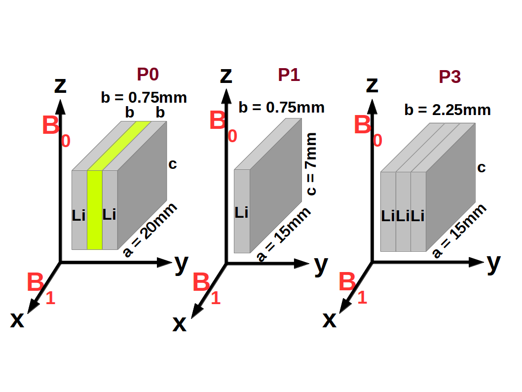
Figure S1: Schematics of MRI phantoms.
Phantoms comprising of Li strips (of dimensions $a\times b\times c$), derived from a 0.75 $mm$ thick stock Li strip.
Phantom P0: Pair of Li strips separated by a teflon strip; For each Li strip, $a\times b\times c=$ 20 x 0.75 x 7 $mm$³.
Phantom P1: Single Li strip. $a\times b\times c=$ 15 x 0.75 x 7 $mm$³.
Phantom P3: Three Li strips pressed together to yield a single composite super strip. $a\times b\times c=$ 15 x 2.25 x 7 $mm$³.
The static (main) magnetic field $\bf B_{0}$ specifies the $z$ direction. Also, $x,y,z$ denote the MRI gradient (imaging) directions. The setup of phantom, r.f. coil and the gradient assembly guarantees that $x\parallel a\parallel\mbox{$\bf B_{1}$}$, with a rotational degree of freedom about the $x$-axis, to reorient the phantom. See sections 1 and 6.1.

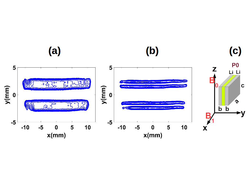
Figure S2: Resolution and strip thickness in bulk metal MRI.
⁷Li 2d MRI(xy) from phantom P0 comprising of two Li strips (separated by a teflon strip) of identical thickness, at (a) 0.5 $mm$ (b) 0.25 $mm$ resolution, along $y$.
For the lower resolution image in panel (a), the extent of image intensity bands along $y$ is mainly determined by the image resolution. It is difficult to infer the strip thickness with any confidence.
On the other hand, for the higher resolution image in panel (b), each conducting strip gives rise to two bands, from the $ac$ faces $\parallel\mbox{$\bf B_{1}$}$; the relative magnitudes of strip thickness, skin-depth and resolution conspire and combine to resolve the faces of each strip. The intra strip band separation yields the thickness of that strip.
See section SS8.1.

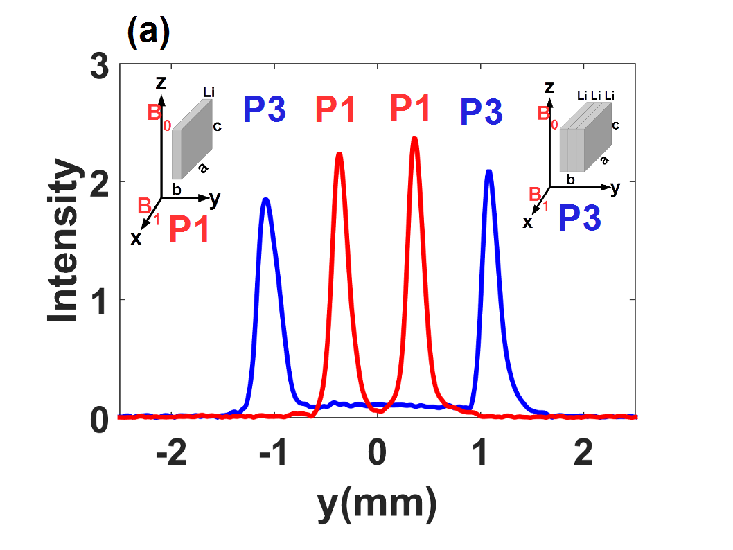
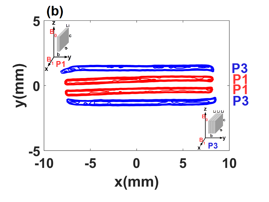
Figure S3: Comparing thickness of strips from bulk metal MRI.
Superpositon of ⁷Li MRI from phantoms P1 and P3. (a) 1d MRI(y). The resolution along $y$, is 0.0357 $mm$. (b) 2d MRI(xy). The resolution along $y$, is 0.250 $mm$.
$x,y,z$ are the imaging directions (Fig.S1). Each phantom gives rise to two bands emanating from its pair of $ac$ faces. Thickness of a given strip is given by the separation, along $y$, between bands arising from it. Mere visual inspection of the panels, by virtue of the equal spacing between the 4 bands along y, suggests that P3 is thrice the thickness of P1. See section SS8.2.

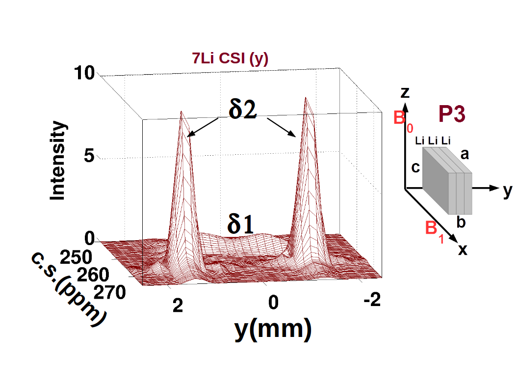
Figure S4: ⁷Li 2d CSI($y$) of phantom P3.
Stack plot representation (intensity along the vertical axis). See also Fig.5 and Fig.S1. Chemical shift along one axis, and image along $y$, comprise the 2 dimensions. Along $y$, the CS at $\delta_{2}$ gives rise to a pair of separated bands, while an extended, low intensity band spanning them is obtained with a CS of $\delta_{1}$. See section 3.

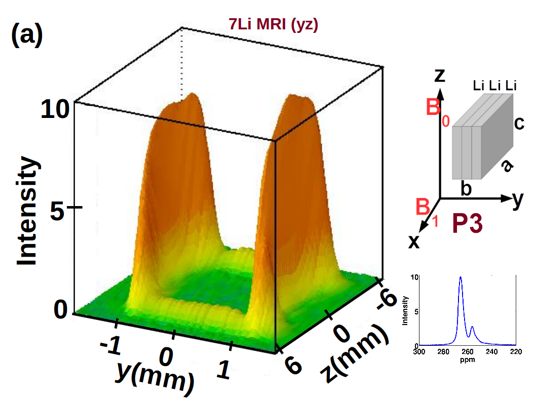
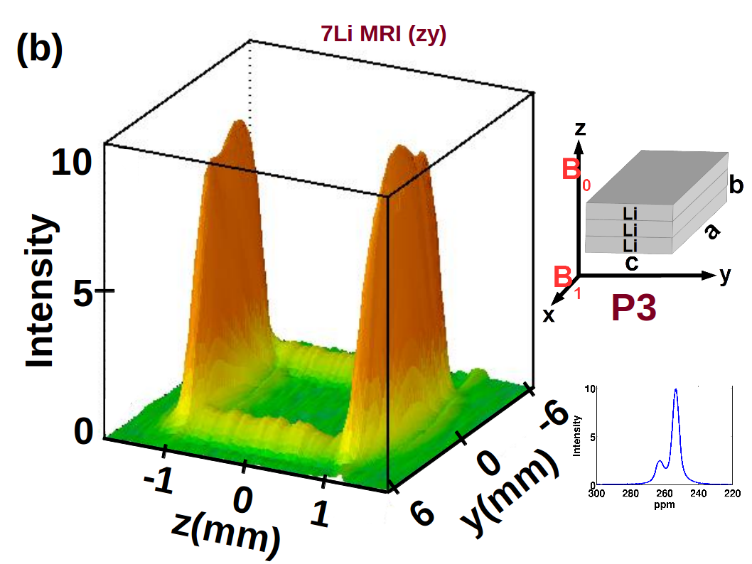
Figure S5: Bulk metal MRI of phantom P3, at mutually orthogonal orientations.
Comparison of ⁷Li 2d MRI stack plots (vertical axis denotes intensity) of phantom P3 in two different orientations.
(a) 2d MRI($yz$) in vertical orientation. (b) 2d MRI($zy$) in horizontal orientation. The corresponding NMR spectra are shown as insets. These images declare a virtual dead heat, between the two orientations, regarding the relative intensities from the two pairs of $ac$ and $ab$ faces. This puts to rest the possibility that the differences in the intensities from the $ab$ and $ac$ faces, arises due to the differing extents to which the eddy currents (arising from the gradient switching in MRI experiments) may affect the signals from the $ab$ and $ac$ faces. See sections 4, 6.2 and SS9.

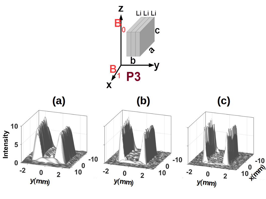
Figure S6: Resolution, and relative signal intensities from $ab$ and $ac$ faces.
⁷Li 2d MRI($xy$) stack plots (intensity along the vertical axis) of phantom P3, at differing resolutions along $y$, providing experimental verification that the ratio of signals from $ac$ and $ab$ faces, increases with increasing resolution (Eq.(5) in section 4).
(a), (b), (c) are respectively at resolutions of 0.5, 0.25 and 0.125 $mm$ along $y$ (Methods section 6.2).

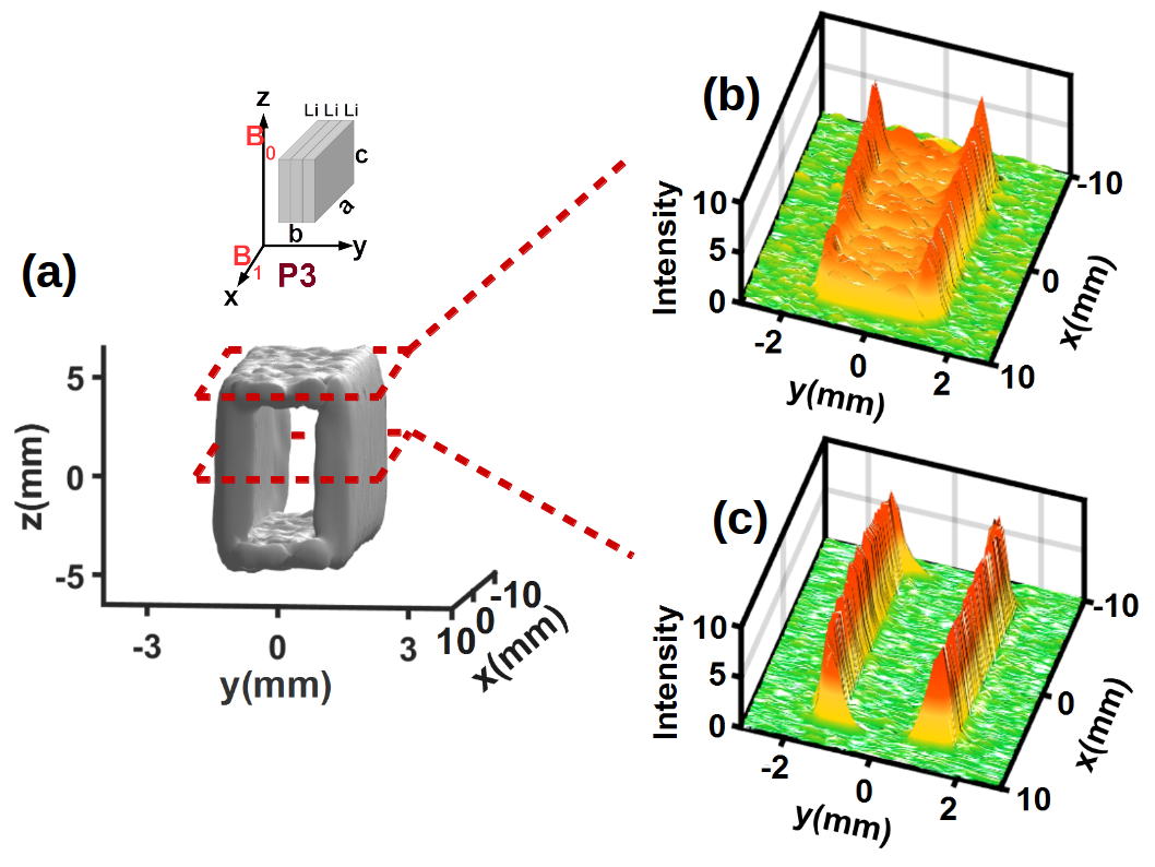
Figure S7: 2d($xy$) slices from MRI($xyz$) of a bulk metal strip.
Visualization of $S_{ab}\neq S_{ac}$ (the signal intensities from $ab$ and $ac$ faces) via 2d ($xy$) slices (along $z$) from ⁷Li 3d MRI($xyz$), of phantom P3 (Fig.S1).
(a) 3d MRI($xyz$); same data as in Fig.3. (b) Slice from the top $ab$ face. (c) Central slice.
The slices are displayed as stack plots (intensity along vertical axis). In a given slice, intensities at all points ($x,y$) are for the same $z$ value in panel (a).
In either slice, the walls of intensity arise from $ac$ faces. The plateau spanning them in panel (b), emanates from the top $ab$ face.
See section 4.

References

-
[1]
J. D. Jackson.
Classical Electrodynamics.
(1990), 3rd edition, John Wiley & Sons, Inc. - [2] David J. Griffiths. Introduction to Electrodynamics. (1999) 3rd edition, Pearson Education Inc., Upper Saddle River, New Jersey, 07458, USA.
- [3] Fawwaz T. Ulaby. Fundamentals of Applied Electromagnetics. (1997), 2001 media edition, Prentice-Hall Inc., Upper Saddle River, New Jersey, 07458, USA.
-
[4]
Rangeet Bhattacharyya, Baris Key, Hailong Chen, Adam S. Best,
Anthony F. Hollenkamp, Clare P. Grey.
In situ NMR observation of the formation of metallic lithium microstructures in lithium batteries.
Nature Materials, (2010), 9, 504-510. -
[5]
S. Chandrashekar, Nicole M. Trease, Hee Jung Chang, Lin-Shu Du, Clare P. Grey
and Alexej Jerschow.
7Li MRI of Li batteries reveals location of microstructural lithium.
Nature Materials, (2012), 11, 311-315. -
[6]
Andrew J. Ilott, S. Chandrashekar, Andreas Kloeckner, Hee Jung Chang,
Nicole M. Trease, Clare P. Grey, Leslie Greengard, Alexej Jerschow.
Visualizing skin effects in conductors with MRI: 7Li MRI experiments and calculations.
J. Magn. Reson., (2014), 245, 143-149. -
[7]
Konstantin Romanenko, Maria Forsyth, Luke A. O’Dell.
New opportunities for quantitative and time efficient 3D MRI of liquid and solid electrochemical cell components: Sectoral Fast Spin Echo and SPRITE.
J. Magn. Reson., (2014), 248, 96-104. -
[8]
M. M. Britton.
Magnetic resonance imaging of electrochemical cells containing bulk metal.
Chem. Phys. Chem., (2014), 15, 1731-1736. -
[9]
Hee Jung Chang, Andrew J. Ilott, Nicole M. Trease, Mohaddese Mohammadi,
Alexej Jerschow, and Clare P. Grey.
Correlating microstructural lithium metal growth with electrolyte salt depletion in lithium batteries using 7Li MRI.
J. Am. Chem. Soc., (2015), 137, 15209-15216. -
[10]
Vincent Perrin.
MRI Techniques.
(John Wiley & Sons, 2013.) -
[11]
Thomas E. Yankeelov, David R. Pickens, Ronald R. Price.
Quantitative MRI in Cancer.
(CRC Press, 2011.) -
[12]
Paul T. Callaghan.
Principles of Nuclear Magnetic Resonance Microscopy.
(2003), Oxford University Press. -
[13]
B. Blumich.
NMR Imaging of Materials.
(Oxford University Press, 2003.) -
[14]
V. S. Bajaj, J. Paulsen, E. Harel and A. Pines.
Zooming in on microscopic flow by remotely detected MRI.
Science, (2010), 330, 1078-1081. -
[15]
D. Rugar, H. J. Mamin, M. H. Sherwood, M. Kim, C. T. Rettner, K. Ohno and
D. D. Awschalom.
Proton magnetic resonance imaging using a nitrogen-vacancy spin sensor.
Nature Nanotechnology, (2015), 10, 120-124. -
[16]
A. J. Davenport, M. Forsyth and M. M. Britton.
Visualisation of chemical processes during corrosion of zinc using magnetic resonance imaging.
Electrochem. Commun., (2010), 12, 44-47. -
[17]
Andrew J. Ilott, Nicole M. Trease, Clare P. Grey, and Alexej Jerschow.
Multinuclear in situ magnetic resonance imaging of electrochemical double-layer capacitors.
Nature Communications, (2014), DOI: 10.1038/ncomms5536. -
[18]
R. E. Gerald II, R. J. Klingler, G. Sandi, C. S. Johnson, L. G. Scanlon and
J. W. Rathke.
7Li NMR study of intercalated lithium in curved carbon lattices.
J. Power Sources, (2000) 89, 237-243. -
[19]
M. Mole, S-I. Han, W.R. Myers, S-K. Lee, N. Kelso, M. Hatridge,
A. Pines, J. Clarke.
SQUID-detected microtesla MRI in the presence of metal.
J. Magn. Reson., (2006), 179, 146-151. -
[20]
C. R. Camacho, D. B. Plewes, R. M. Henkelman.
Nonsusceptibility artifacts due to metallic objects in MR-imaging.
J. Magn. Reson. Imaging, (1995), 5, 75-88. - [21] L. H. Bennett, P. S. Wang, M. J. Donahue. Artifacts in magnetic resonance imaging from metals. J. App. Phys. (1996), 79, 4712-4714.
- [22] R. V. Olsen, P. L. Munk, M. J. Lee, D. L. Janzen, A. L. MacKay, Q. S. Xiang, B. Masri. Metal artifact reduction sequence: Early clinical applications. Radiographics, (2000), 20, 699-712.
- [23] M. J. Lee, D. L. Janzen, P. L. Munk, A. MacKay, Q-S Xiang, A. McGowan. Quantitative assessment of an MR technique for reducing metal artifact: application to spin-echo imaging in a phantom. Skeletal Radiol, (2001), 30, 398-401.
- [24] A. M. Viano, S. A. Gronemeyer, M. Haliloglu, F. A. Hoffer. Improved MR imaging for patients with metallic implants. Magn. Reson. Imag., (2000), 18, 287-295.
- [25] F. Shafiei, E. Honda, H. Takahashi, and T. Sasaki. Artifacts from dental casting alloys in magnetic resonance imaging. J. Dent. Res,. (2003), 82, 602-606.
- [26] H. Graf, G. Steidle, P. Martirosian, U. A. Lauer, F. Schick. Effects on MRI due to altered RF polarization near conductive implants or instruments. Med. Phys., (2006), 33, 124-127.
- [27] K. M. Koch, B. A. Hargreaves, K. Butts Pauly, W. Chen, G. E. Gold, K. F. King. Magnetic resonance imaging near metal implants. J. Magn. Reson. Imaging, (2010), 32, 773-778.
- [28] Joseph F. Zikria, Stephen Machnicki, Eugene Rhim, Tandeep Bhatti, Robert E. Graham. MRI of Patients With Cardiac Pacemakers: A review of the medical literature. American Journal of Roentgenology (2011), 196, 390-401.
- [29] Djaudat Idiyatullin, Curt Corum, Steen Moeller, Hari S. Prasad, Michael Garwood, and Donald R. Nixdorf. Dental MRI: Making the invisible visible. J. Endod. (2011) 37, 745-752.
- [30] Michael Garwood. MRI of fast-relaxing spins. J. Magn. Reson. (2013), 229, 49-54.
- [31] M. M. Britton, P. M. Bayley, P. C. Howlett, A. J. Davenport, M Forsyth. In-situ real time visualization of electrochemistry using magnetic resonance imaging. J. Phys. Chem. Lett., (2013), 3019-3023.
- [32] M. Klett, M. Giesecke, A. Nyman, F. Hallberg, K. W. Lindstrom, G. Lindbergh, I. Furo. Quantifying mass transport during polarization in a li ion battery by in-situ 7Li NMR imaging. J. Am. Chem. Soc., (2012), 134, 14654-14657.
- [33] M. Giesecke, S. V. Dvinskikh and I. Furo. Constant-time chemical-shift selective imaging. J. Magn. Reson., (2013), 226, 19-21.
-
[34]
E. Mark Haacke, Robert E. Brown, Michael R. Thompson and
Ramesh Venkatesan.
Magnetic Resonance Imaging: Physical Principles and Sequence Design.
(1999) John Wiley & Sons, Inc. - [35] Nils Spengler, Jens Hoefflin, Ali Moazenzadeh, Dario Mager, Neil MacKinnon, Vlad Badilita, Ulrike Wallrabe, Jan G. Korvink. Heteronuclear micro-Helmholtz coil facilitates m-range spatial and sub-Hz spectral resolution NMR of nL-volume samples on customisable microfluidic chips. PLoS ONE, (2016), 11, doi:10.1371/journal.pone.0146384.
- [36] Kirk W. Feindel. Spatially resolved chemical reaction monitoring using magnetic resonance imaging. Magn. Reson. Chem., (2015), doi:10.1002/mrc.4179.
-
[37]
R. E. Hoffman.
Measurement of magnetic susceptibility and calculation of shape factor of NMR samples.
J. Magn. Reson. (2006), 178, 237-247. -
[38]
Lina Zhou, Michal Leskes, Andrew J. Ilott, N. M. Trease, Clare P. Grey
Paramagnetic electrodes and bulk magnetic susceptibility effects in the in situ NMR studies of batteries: application to Li1.08Mn1.92O4 spinels.
J. Magn. Reson. (2013), 234, 44-57. -
[39]
Hee Jung Chang, Nicole M. Trease, Andrew J. Ilott, Dongli Zeng, Lin-Shu Du,
Alexej Jerschow, and Clare P. Grey.
Investigating Li microstructure formation on Li anodes for lithium batteries by in situ 6Li/7Li NMR and SEM.
J. Phys. Chem. C, (2015), 119, 16443-16451. -
[40]
Jose A. Rodriguez, D. Wayne Goodman.
The nature of the metal-metal bond in bimetallic surfaces.
Science (1992) 257 897-903. -
[41]
C. P. Flynn.
Point defect reactions at surfaces and in bulk metals.
Physical Review B (2005) 71 085422. -
[42]
L. Gireaud, S. Grugeon, S. Laruelle, B. Yrieix and J. M. Tarascon.
Lithium metal stripping/plating mechanisms studies: A metallurgical approach.
Electrochem. Commun., (2006), 8, 1639-1649. -
[43]
B.P.P.A. Gouveia, J.M.C. Rodrigues, P.A.F. Martins.
Fracture predicting in bulk metal forming.
International Journal of Mechanical Sciences (1996) 38 361-372. -
[44]
M. Mavrikakis, B. Hammer, J. K. Norskov.
Effect of Strain on the Reactivity of Metal Surfaces.
Physical Review Letters (1998) 81 2819-2822. -
[45]
C. J. Zhong et. al.
Nanostructured catalysts in fuel cells.
Nanotechnology, (2010), 21, 062001. -
[46]
Fang-Wei Yuan, Hong-Jie Yang, Hsing-Yu Tuan.
Seeded silicon nanowire growth catalyzed by commercially available bulk metals: broad selection of metal catalysts, superior field emission performance, and versatile nanowire/metal architectures.
Journal of Materials Chemistry (2011) 21 13793-13800. -
[47]
S. Talapatra, S. Kar, S. K. Pal, R. Vajtai, L. Ci, P. Victor, M. M. Shaijumon,
S. Kaur, O. Nalamasu and P. M. Ajayan.
Direct growth of aligned carbon nanotubes on bulk metals.
Nature Nanotechnology (2006) 1 112-116. -
[48]
J. L. Whitten, H. Yang.
Theory of chemisorption and reactions on metal surfaces.
Surface Science Reports (1996) 24 55-57. -
[49]
Robert G. Greenler.
Infrared Study of Adsorbed Molecules on Metal Surfaces by Reflection Techniques.
The Journal of Chemical Physics (1966) 44 310-315. -
[50]
A. Abragam.
Principles of nuclear magnetism.
(1961), Oxford University Press, London. - [51] D. R. Lide & H. P. R. Frederikse. CRC Handbook of Chemistry and Physics: A Ready-Reference Book of Chemical and Physical Data. 78th edn. (1997), CRC Press.
- [52] R. R. Ernst, G. Bodenhausen and A. Wokaun. Principles of Nuclear Magnetic Resonance in One and Two Dimensions. (1987), Oxford University Press.
- [53] W. M. Saslow. Maxwell’s theory of eddy currents in thin conducting sheets, and applications to electromagnetic shielding and MAGLEV. Am. J. Phys. (1992), 60, 693-711.
- [54] William Wallace Brey. (2014) Private communication.
- [55] S. Vashaee, F. Goora, M. M. Britton, B. Newling, B. J. Balcom. Mapping B1-induced eddy current effects near metallic structures in MR images: A comparison of simulation and experiment. J. Magn. Reson. (2015), 250, 17-24.
- [56] Dye J. Jensen, William W. Brey, Jean L. Delayre, Ponnada A. Narayana. Reduction of pulsed gradient settling time in the superconducting magnet of a magnetic resonance instrument. Med. Phys., (1987), 14, 859.