Identifying the order of a quantum phase transition by means of Wehrl entropy in phase-space

Abstract

We propose a method to identify the order of a Quantum Phase Transition by using area measures of the ground state in phase space. We illustrate our proposal by analyzing the well known example of the Quantum Cusp, and four different paradigmatic boson models: Dicke, Lipkin-Meshkov-Glick, interacting boson model, and vibron model.

I Introduction

The extremely relevant concept of phase transition in Thermodynamics has been extended in later times to encompass novel situations. In particular, two main aspects have been recently addressed: the study of mesoscopic systems and of quantum systems at zero temperature. In the first case, the finite system size modifies and smooths phase transition effects. In the second case a tiny modification of certain Hamiltonian parameter or parameters (control parameters) induces an abrupt change in the ground state of the quantum system and Quantum Phase Transitions (QPTs) appear as an effect of quantum fluctuations at the critical value of the control parameter Carr (2010). QPTs strictly occur in infinite systems, though QPT precursors are present in finite systems. In fact, bosonic models allow to study both aforementioned aspects: finite-size effects and zero temperature QPTs. Recent reviews on this subject are Casten (2009); Cejnar and Jolie (2009); Cejnar et al. (2010).

QPTs occurring in finite-size systems can be characterized by the disappearance of the gap between the ground and the first excited state energies in the mean field or thermodynamic limit (infinite system size). The QPT is a first order phase transition if a level crossing occurs and a continuous transition if there are no crossings (except in the limit value) Cejnar et al. (2007). The Landau theory holds in the models addressed in this presentation, and within this theory the Ehrenfest classification of QPTs is valid. In this case, the order of a QPT is assigned on the basis of discontinuities in derivatives of the potential of the system at the thermodynamic limit Cejnar and Jolie (2009); Cejnar et al. (2010).

The assignment of the order of a phase transitions in finite-size systems using a numerical treatment to compute finite differences of the system energy functional can be a cumbersome task. In order to overcome this problem, different approaches have been proposed. Cejnar et al. have used the study of nonhermitian degeneracies near critical points to classify the order of QPTs Cejnar et al. (2007). Alternative characterizations are based in the connection between geometric Berry phases and QPTs in the case of the XY Ising model Carollo and Pachos (2005); Zhu (2006) and in the overlap between two ground state wave functions for different values of the control parameter (fidelity susceptibility concept) Zanardi and Paunković (2006); Gu (2010); Pérez-Campos et al. (2010). In addition, many efforts have been devoted to characterize QPTs in terms of information theoretic measures of delocalization (see Nagy and Romera (2012); Romera et al. (2013, 2012a); Nagy and Romera (2015) and references therein) and quantum information tools, e. g. using entanglement entropy measures (see e.g. Lambert et al. (2005) for the Dicke model and Calixto et al. (2012a); Calixto and Pérez-Bernal (2014) for the vibron model).

In this work we propose an alternative way to reckon the order of a QPT by using the Wehrl entropy in the phase-space (coherent state or Bargmann) representation of quantum states $\psi$ provided by the Husimi function $Q_{\psi}$, which is defined as the squared overlap between $\psi$ and an arbitrary coherent state.

The Husimi function has been widely used in quantum physics, mainly in quantum optics. For example, the time evolution of coherent states of light in a Kerr medium is visualized by measuring $Q_{\psi}$ by cavity state tomography, observing quantum collapses and revivals, and confirming the non-classical properties of the transient states Kirchmair et al. (2013). Moreover, the zeros of this phase-space quasi-probability distribution have been used as an indicator of the regular or chaotic behavior in quantum maps for a variety of quantum problems: molecular Arranz et al. (2010) and atomic Dando and Monteiro (1994) systems, the kicked top Chaudhury et al. (2009), quantum billiards Tualle and Voros (1995), or condensed matter systems Weinmann et al. (1999) (see also Leboeuf and Voros (1990); Arranz et al. (2013) and references therein). They have also been considered as an indicator of metal-insulator Aulbach et al. (2004) and topological-band insulator Calixto and Romera (2015) phase transitions, as well as of QPTs in Bose Einstein condensates Pérez-Campos et al. (2010) and in the Dicke del Real et al. (2013); Romera et al. (2012b), vibron Calixto and Pérez-Bernal (2014), and Lipkin-Meshkov-Glick (LMG) models Romera et al. (2014).

To identify the order of a QPT we suggest to observe the singular behavior of the Wehrl entropy, $W_{\psi}$, of the Husimi function, $Q_{\psi}$, near the critical point as the system size increases. The Wehrl entropy, is defined in Sec. III as a function of the Hamiltonian control parameter(s) and the system’s size. For harmonic oscillators, Lieb proved in Lieb (1978) the Wehrl’s conjecture Wehrl (1979) stating that $W_{\psi}$ attains its minimum (maximum area) when $\psi$ is an ordinary (Heisemberg-Weyl) coherent state. This proof has been recently extended by Lieb and Solovej to SU(2) spin-$j$ systems Lieb and Solovej (2014). We observe that $W_{\psi}$ is maximum at the critical point of a first-order QPT, and this maximum is narrower as the system size increases. However, for second-order QPTs, the Wehrl entropy displays a step function behavior at the critical point, and again the transition is sharper for larger system sizes. We shall confirm this behavior for five models: Quantum Cusp, Dicke, LMG, a one-dimensional realization of the interacting boson model (IBM-LMG), and the 2D limit of the vibron model (2DVM).

We have chosen the Cusp model as a prototypical case, because this is probably the best known catastrophe example, describing the bifurcation of a critical point with a quartic potential. Its quantum version Gilmore et al. (1986) has been used to illustrate the effects associated with criticality as a prior step to deal with more involved physical situations Cejnar and Stránský (2008); Cejnar and Jolie (2009); Gilmore et al. (1986); Emary et al. (2005). In addition to the Cusp model, we present results for four different realizations of bosonic systems. The LMG model is a simple model, originally introduced for the description of nuclear systems as an exactly-solvable toy model to assess the quality of different approximations Lipkin et al. (1965). This ubiquitous model still receives a major attention, further stimulated by its recent experimental realization Jurcevic et al. (2014); Richerme et al. (2014). The study of the ground state quantum phase transitions for this model can be traced back to the seminal articles of Gilmore and Feng Gilmore and Feng (1978a, b). The Dicke model is a quantum-optical model that describes the interaction of a radiation field with $N$ two-level atoms Dicke (1954). This model has recently renewed interest Garraway (2011); Castaños et al. (2011a, b); Nataf and Ciuti (2010), partly because a tunable matter-radiation interaction is a keynote ingredient for the study of quantum critical effects Lambert et al. (2005); Emary and Brandes (2003a, b) and partly because the model phase transition has been observed experimentally Baumann et al. (2010). The interacting boson model (IBM) was introduced by Arima and Iachello to describe the structure of low energy states of even-even medium and heavy nuclei Iachello and Arima (1987). For the sake of simplicity, we use the IBM-LMG, a simplified version of the model built with scalar bosons Vidal et al. (2006). Finally, the vibron model was also proposed by Iachello to describe the rovibrational structure of molecules Iachello (1981) and the 2DVM was introduced Iachello and Oss (1996) to model molecular bending dynamics (e.g. see Ref. Larese et al. (2013) and references therein). The 2DVM is the simplest two-level model which still retains a non-trivial angular momentum quantum number and it has been used as a playground to illustrate ground state and excited state QPTs features in bosonic models Caprio et al. (2008); Pérez-Bernal and Iachello (2008).

We proceed to present the Hamiltonian of the five different addressed models, defining the Wehrl entropy as functions of the moments of the Husimi function $Q_{\psi}$, and the results obtained in the first and second order critical points of the different models considered. A brief introduction to the main results on Schwinger boson realizations, coherent states, and energy surfaces used in the paper can be found in App. A.

II Selected Models

We give a brief outline of the five models we use to illustrate the characterization of QPT critical points by means of the Wehrl entropy.

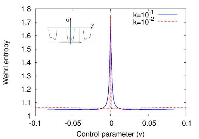
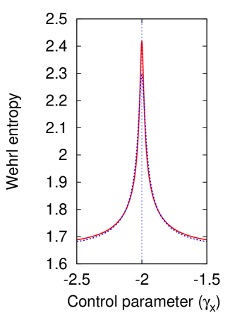
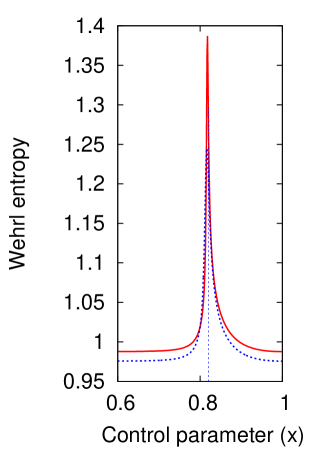
Figure 1: (Color online) First order QPTs: Wehrl entropy $W_{\psi}$ of the Husimi function for the ground state. Top panel: cusp model for $k=10^{-1}$ (blue, solid) and $10^{-2}$ (red, dashed), along the straight line $u=-1$ with critical point $v_{c}=0$. Bottom left: LMG model for $N=20$ (blue, dashed) and $40$ (red, solid), along the straight line $\gamma_{x}=-\gamma_{y}-4$ with critical point $\gamma_{xc}=-2$. Bottom right: IBM-LMG model for $N=80$ (red, solid) and $N=40$ (blue, dashed), for the straight line $y=\frac{1}{\sqrt{2}}$ with critical point $x_{c}=0.82$. Critical points are marked with vertical blue dotted lines.

The first model is the one dimensional quantum cusp Hamiltonian Gilmore et al. (1986); Cejnar and Stránský (2008); Cejnar and Jolie (2009); Emary et al. (2005)

$$\hat{H}=\frac{K^{2}{\hat{p}}^{2}}{2}+V_{c}(\hat{x})~{},$$ (1)

where $V_{c}(\hat{x})=\frac{1}{4}{\hat{x}}^{4}+\frac{u}{2}{\hat{x}}^{2}+v\hat{x}$ is the cusp potential, with control parameters $u$ and $v$ and a classicality constant $K=\frac{\hbar}{\sqrt{M}}$, combining $\hbar$ and the mass parameter $M$ (see Cejnar and Stránský (2008)). The smaller the value of $K$ the closer the system is to the classical limit. The mass parameter $M$ can be fixed to unity without loss of generality. In order to obtain energies and eigenstates for the quantum Cusp, we have recast Hamiltonian (1) in second quantization, using harmonic oscillator creation and annihilation operators, and diagonalized the resulting matrix with a careful assessment of convergence. The ground state quantum phase transitions associated with the cusp have been studied using Catastrophe Theory and Ehrenfest’s classification Cejnar and Jolie (2009) and making use of entanglement singularities Emary et al. (2005). It is well known that there is a first order quantum phase transition line when the control parameter $v$ changes sign for negative $u$ values, and a second order transition point for $v=0$ and $u$ moving from negative to positive values. In this work we will consider two trajectories: (i) for $u=-1$ and $v\in[-0.2,0.2]$ with a first order critical point at $v_{c}=0$, and (ii) for $v=0$ and $u\in[-1,1]$ with a second order critical point at $u_{c}=0$.

The Dicke model is an important model in quantum optics that describes a bosonic field interacting with an ensemble of $N$ two-level atoms with level-splitting $\omega_{0}$. The Hamiltonian is given by

$$\hat{H}=\omega_{0}{\hat{J}}_{z}+\omega a^{{\dagger}}a+\frac{\lambda}{\sqrt{2j}}(a^{{\dagger}}+a)({\hat{J}}_{+}+{\hat{J}}_{-})~{},$$ (2)

where ${\hat{J}}_{z}$, ${\hat{J}}_{\pm}$ are angular momentum operators for a pseudospin of length $j=N/2$, and $a$ and $a^{{\dagger}}$ are the bosonic operators of a single-mode field with frequency $\omega$. There is a second order QPT at a critical value of the atom-field coupling strength $\lambda_{c}=\frac{1}{2}\sqrt{\omega\omega_{0}}$, with two phases: the normal phase ($\lambda<\lambda_{c}$) and the superradiant phase ($\lambda>\lambda_{c}$) Hepp and Lieb (1973); Wang and Hioe (1973). Several tools for the identification of its QPTs have been proposed: by means of entanglement Lambert et al. (2005), information measures (see Romera et al. (2012a); Nagy and Romera (2012) and references therein) and in terms of fidelity Castaños et al. (2012), inverse participation ratio, the Wehrl entropy and the zeros of the Husimi function and marginals Romera et al. (2012b); del Real et al. (2013); Bastarrachea-Magnani et al. (2015).

We will also deal with an interacting fermion-fermion model, the LMG model Lipkin et al. (1965). In the quasispin formalism, except for a constant term, the Hamiltonian for $N$ interacting spins can be written as

$$\frac{\hat{H}}{2\omega j}=\frac{{\hat{J}}_{z}}{j}+\frac{\gamma_{x}}{j(2j-1)}{\hat{J}}^{2}_{x}+\frac{\gamma_{y}}{j(2j-1)}{\hat{J}}^{2}_{y}~{},$$ (3)

where $\gamma_{x}$ and $\gamma_{y}$ are control parameters. We would like to point out that the total angular momentum $J^{2}=j(j+1)$ and the number of particles $N=2j$ are conserved, and $\hat{H}$ commutes with the parity operator for fixed $j$. Ground state quantum phase transitions for this model have been characterized using the continuous unitary transformation technique Dusuel and Vidal (2004), investigating singularities in the complex plane (exceptional points) Heiss et al. (2005), and from a semiclassical perspective Leyvraz and Heiss (2005). A complete classification of the critical points has been accomplished using the catastrophe formalism Castaños et al. (2005, 2006). We will study the first and second order QPTs given by the trajectories $\gamma_{x}=-\gamma_{y}-4$ and $\gamma_{x}=-\gamma_{y}+2$ in the phase diagram Castaños et al. (2006). A characterization of QPTs in the LMG model has recently been performed in therms of Rényi-Wehrl entropies, zeros of the Husimi function and fidelity and fidelity suspceptibility concepts Romera et al. (2014).

In the case of the characterization of the phase diagram associated with the IBM it is important to emphasize the pioneer works on shape phase transitions on nuclei Feng et al. (1981), that anticipated the detailed construction of the phase diagram of the interacting boson model using either catastrophe theory Feng et al. (1981); López-Moreno and Castaños (1996), the Landau theory of phase transitions Iachello et al. (1998); Jolie et al. (2002), or excited levels repulsion and crossing Arias et al. (2003). In the present work we use the IBM-LMG, a simplified one dimensional model, which shows first and second order QPTs, having the same energy surface as the Q-consistent interacting boson model Hamiltonian Vidal et al. (2006). In this case the Hamiltonian is

$$\hat{H}=x{\hat{n}}_{t}-\frac{1-x}{N}{\hat{Q}}^{y}{\hat{Q}}^{y}~{},$$ (4)

with ${\hat{n}}_{t}=t^{{\dagger}}t$ and ${\hat{Q}}^{y}=s^{{\dagger}}t+t^{{\dagger}}s+y\,t^{{\dagger}}t$ are expressed in terms of two species of scalar bosons $s$ and $t$, and the Hamiltonian has two control parameters $x$ and $y$. The total number of bosons $N={\hat{n}}_{s}+{\hat{n}}_{t}$ is a conserved quantity. For $y=0$ there is an isolated point of second order phase transition as a function of $x$ with a critical value $x_{c}=0.8$. For $y>0$ the phase transition is of first order and, to illustrate this case, we have chosen the value $y=1/\sqrt{2}$, with a critical control parameter $x_{c}=0.82$.

Finally, the 2DVM is a model which describes a system containing a dipole degree of freedom constrained to planar motion. Elementary excitations are (creation and annihilation) 2D Cartesian $\tau$-bosons and a scalar $\sigma$-boson. The second order ground state quantum phase transition in this model has been studied in Ref. Pérez-Bernal and Iachello (2008) using the essential Hamiltonian

$$\hat{H}=(1-\xi)\hat{n}+\xi\frac{N(N+1)-\hat{W}^{2}}{N-1},$$ (5)

where the (constant) quantum number $N$ labels the totally symmetric representation $[N]$ of U(3), $\hat{n}=\tau_{+}^{\dagger}\tau_{+}+\tau_{-}^{\dagger}\tau_{-}$ is the number operator of vector bosons, and $\hat{W}^{2}=(\hat{D}_{+}\hat{D}_{-}+\hat{D}_{-}\hat{D}_{+})/2+\hat{l}^{2}$. The operators $\hat{D}_{+}=\sqrt{2}(\tau^{\dagger}_{+}\sigma-\sigma^{\dagger}\tau_{-})$ and $\hat{D}_{-}=\sqrt{2}(-\tau^{\dagger}_{-}\sigma+\sigma^{\dagger}\tau_{+})$ are dipole operators, and $\hat{l}=\tau_{+}^{\dagger}\tau_{+}-\tau_{-}^{\dagger}\tau_{-}$ is the angular momentum operator. This model has a single control parameter $0\leq\xi\leq 1$ and the second order QPT takes place at a critical value $\xi_{c}=0.2$ Pérez-Bernal and Iachello (2008). Several procedures have been used to identify the ground state QPT in this model: entanglement entropies Calixto et al. (2012a), Rényi entropies Romera et al. (2013), the Wehrl entropy, and the inverse participation ratio of the Husimi function Calixto et al. (2012b).

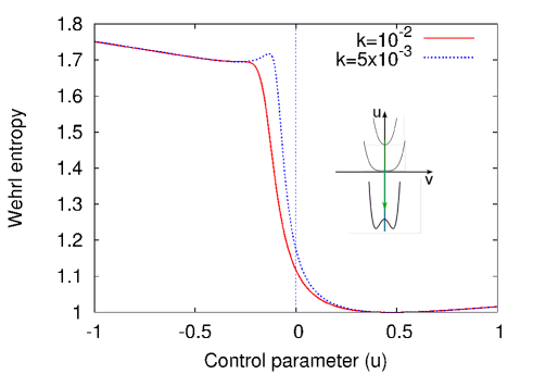
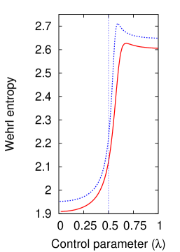
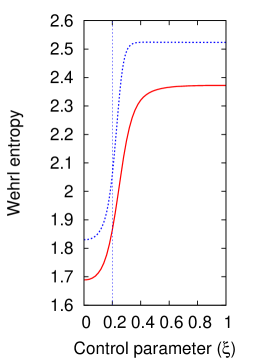
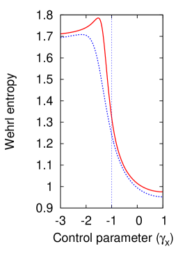
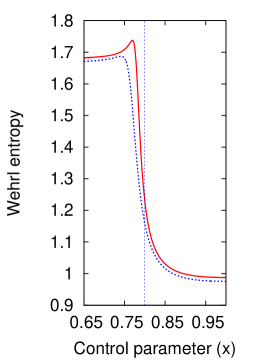
Figure 2: (Color online) Second order QPTs: Wehrl entropy $W_{\psi}$ of the Husimi function for the ground state. Top panel: cusp model for $K=10^{-2}$ (red, solid) and $10^{-3}$ (blue, dashed), along the straight line $u=0$ with critical point $v_{c}=0$. Mid left panel: Dicke model for $N=10$ (red, solid) and $20$ (blue, dashed) with critical point $\lambda_{c}=0.5$; mid right panel: 2DVM results for $N=8$ (red, solid) and $16$ (blue, dashed) with critical point $\xi_{c}=0.2$. Bottom left panel: LMG model for $N=20$ (blue, dashed) and $40$ (red, solid), along the straight line $\gamma_{x}=-\gamma_{y}+2$ with critical point $\gamma_{xc}=-1$. Bottom right panel: IBM-LMG model for $N=80$ (red, solid) and $N=40$ (blue, dashed), for the straight line $y=0$ with critical point $x_{c}=0.8$.

III Wehrl’s entropy and ground state QPTs

We have numerically diagonalized the Hamiltonians of the five models for two different values of the system size $N$ in an interval of control parameters containing a critical point (either first- or second-order). Given the expansion $|\psi\rangle=\sum_{n}c_{n}|n\rangle$ of the ground state in a basis $\{|n\rangle,n\in I\}$ ($I$ denotes a set of quantum indices) with coefficients $c_{n}$ depending on the control parameters and the system’s size $N$, and given the expansions of coherent states $|\zeta\rangle$ in the corresponding basis (see App. A), we can compute the Husimi function $Q_{\psi}(\zeta)=|\langle\zeta|\psi\rangle|^{2}$ and the Wehrl entropy

$$W_{\psi}=-\int Q_{\psi}(\zeta)\ln[Q_{\psi}(\zeta)]d\mu(\zeta),$$ (6)

where we are generically denoting by $d\mu(\zeta)$ the measure in each phase space with points labeled by $\zeta$. Note that $W_{\psi}$ is a function of the control parameters and the system size $N$. We discuss typical (minimum) values of $W_{\psi}$ for each model, which are attained when the ground state $\psi$ is coherent itself, and Wehrl entropy values of parity-adapted (Schrödinger cat) coherent states Castaños et al. (1995); Castaños and Lopez-Saldivar (2012), which usually appear in second-order QPTs Calixto et al. (2012a); Calixto and Pérez-Bernal (2014); del Real et al. (2013); Romera et al. (2014); Castaños et al. (2011a, b).

Cusp: in the top panel of Figs. 1 and 2 we plot $W_{\psi}$ as a function of the control parameters $u$ and $v$ for two trajectories and two values of the classicality constant $K$. The first order case is for trajectory $u=-1$, depicted in Fig. 1, with a critical control parameter $v_{c}=0$. In this case it is immediately apparent a sudden growth of Wehrl entropy of the ground state at the critical point $v_{c}=0$. The entropy growth is sharper as $K$ decreases. The ground state is approximately a coherent state for $v\not=0$ and a cat-like state for $v=0$. Indeed, as conjectured by Wehrl Wehrl (1979) and proved by Lieb Lieb (1978), any Glauber coherent state $|\psi\rangle=|\beta\rangle$ has a minimum Wehrl entropy of $W_{\psi}=1$. It has also been shown Romera et al. (2012b); Calixto et al. (2012a); del Real et al. (2013); Romera et al. (2014) that parity adapted coherent (Schrödinger cat) states, $|\psi\rangle\propto|\beta\rangle+|-\beta\rangle$, increase the minimum entropy by approximately $\ln(2)$ (for negligible overlap $\langle-\beta|\beta\rangle$). With this information, we infer that the ground state $|\psi\rangle$ is approximately a coherent state in the phase $u>0$ and a cat-like state in the phase $u<0$.

The second order QPT case is shown in Fig. 2, with $v=0$ and critical control parameter $u_{c}=0$. For the second trajectory, if we move from positive to negative values of $u$, we find in the top panel of Fig. 2 a sudden growth of $W_{\psi}$ in the vicinity of the critical point $u_{c}=0$ jumping from $W_{\psi}(u>0)\simeq 1$ to $W_{\psi}(u<0)\simeq 1+\ln(2)$. The entropy growth is sharper as $K$ decreases (classical limit).

Therefore, we would like to emphasize the utterly different entropic behavior of first- and second-order QPTs. In both cases we also plot an inset with the parameter trajectory and the evolution of the potential along it. We proceed to show that this Wehrl entropy behavior is shared by the rest of the considered models too, allowing a clear distinction between first and second order QPTs.

LMG: the LMG model has first and second order transitions depicted in the bottom left panels of Figs. 1 and 2, respectively. We plot $W_{\psi}$ as a function of the control parameters $\gamma_{x}$ and $\gamma_{y}$ for the trajectories: $\gamma_{y}=-\gamma_{x}-4$ (1^st order QPT at $\gamma_{xc}=-2$, bottom left panel Fig. 1) and $\gamma_{y}=-\gamma_{x}+2$ (2^nd order QPT at $\gamma_{xc}=-1$, bottom left panel Fig. 2), for two values of the total number of particles $N$. We observe an entropic behavior completely similar to the Cusp model. The difference only lies on the particular entropy values. In fact, according to Lieb’s conjecture Lieb (1978); Lieb and Solovej (2014)), spin-$j$ coherent states have a minimum Wehrl entropy of $W_{\psi}=\frac{2j}{2j+1}$, which tends to $W_{\psi}=1$ in the thermodynamic limit $j\to\infty$. Cat-like states again increase the minimum entropy by approximately $\ln(2)$. The IBM-LMG model exhibits a similar behavior to the LMG model, as can be appreciated in the bottom right panel of Figs. 1 and 2.

Dicke: the Dicke model exhibits a 2nd-order QPT at the critical value of the control parameter $\lambda_{c}=0.5$, when going from the normal ($\lambda<\lambda_{c}$) to the superradiant ($\lambda>\lambda_{c}$) phase. $W_{\psi}$ captures this transition, as it can be seen in the mid left panel of Fig.  2, showing an entropy increase from $W_{\psi}\simeq 1+\frac{N}{N+1}$ to $W_{\psi}\simeq 1+\frac{N}{N+1}+\ln(2)$, with $N=2j$ the number of atoms. As expected, the entropic growth at $\lambda_{c}$ is sharper for higher $N$.

Vibron: the vibron model undergoes a 2nd-order (shape) QPT at $\xi_{c}=0.2$, the critical point that marks a change between linear ($\xi<\xi_{c}$) and bent ($\xi>\xi_{c}$) phases Pérez-Bernal and Iachello (2008). In the mid right panel of Fig. 2 we plot the Wehrl entropy as a function of $\xi$ for two values of the system’s size $N$ (total number of bosons). As in the previous models, the 2nd-order QPT is characterized by a “step function” behavior of $W_{\psi}$ near the critical point. In this case, we have conjectured Calixto et al. (2012a) that minimum entropy $W_{\psi}=\frac{N(3+2N)}{(N+1)(N+2)}$ is attained for U(3) coherent states. In the bent phase, the ground state $|\psi\rangle$ is a cat Calixto et al. (2012a, b); Calixto and Pérez-Bernal (2014) and therefore $W_{\psi}\simeq\frac{N(3+2N)}{(N+1)(N+2)}+\ln(2)$.

IV Concluding remarks

In summary, we have numerically diagonalized the Hamiltonians of five models for several system’s sizes $N$ in a given interval of control parameters that contains a critical point (either of first or second order). Given the expansion $|\psi\rangle=\sum_{n}c_{n}|n\rangle$ of the ground state in a basis $\{|n\rangle,n\in I\}$ ($I$ denotes a set of quantum indices) with coefficients $c_{n}$ depending on the control parameters and the system’s size $N$, and given the expansions of coherent states in the corresponding basis, we can compute the Husimi function $Q_{\psi}$ and the Wehrl entropy $W_{\psi}$. In Figs. 1 and 2 we plot $W_{\psi}$ as a function of a control parameter for different values of $N$.

From the obtained results it is clear that the Wehrl entropy behavior at the vicinities of the critical point is an efficient numerical way of distinguishing first order and continuous QPTs.

It is worth to emphasize that the present approach could imply an extra computational cost if compared to the search of nonanaliticities in the ground state energy functional. The present method makes use of the ground state wave functions for different values of the control parameter and it also requires the calculation of the overlap of the basis states with the coherent states. Though the need of ground state wavefunctions instead of ground state energies is computationally more exigent, the finer sensitivity of the present method largely offsets the extra computational cost. The second step, the overlap with coherent states, needs to be done only once with available analytic expressions (see App. A), therefore it does not constitute a significant computational burden. The proposed approach permits a clear determination of the character of a critical point using relatively small basis sets. On the contrary, even for large system sizes, the numerical determination with finite differences of the critical points character could remain ambiguous.

A similar sensitivity and computational cost could be attained with the fidelity susceptibility approach, that provides a clear determination of the critical point location, but with no information of the transition order and with the additional hindrance of varying the control parameter in two different scales. Something similar happens with entanglement entropy measures, that are suitable to be applied to bipartite or multipartite systems, the critical point is clearly located but no precise information about the transition order is obtained.

Appendix A Schwinger boson realizations, coherent states and energy surfaces

Single mode

radiation fields are described by harmonic oscillator creation $a^{\dagger}$ and annihilation $a$ operators in Fock space $\{|n\rangle=\frac{(a^{\dagger})^{n}}{\sqrt{n!}}|0\rangle\}$, and the corresponding normalized coherent state (CS) is given by:

$$|\alpha\rangle=e^{-|\alpha|^{2}/2}e^{\alpha a^{\dagger}}|0\rangle=e^{-|\alpha|^{2}/2}\sum_{n=0}^{\infty}\frac{\alpha^{n}}{n!}|n\rangle,$$ (7)

where $\alpha=x+ip\in\mathbb{C}$ is given in terms of the quadratures $x,p$ of the field. The phase space (Bargmann) representation of a given normalized state $|\psi\rangle=\sum_{n=0}^{\infty}c_{n}|n\rangle$ of the (single mode) radiation field is given by the Husimi function $Q_{\psi}(\alpha)=|\langle\alpha|\psi\rangle|^{2}$, which is normalized according to $\int_{\mathbb{R}^{2}}Q_{\psi}(\alpha)d\mu(\alpha)=1$, with measure $d\mu(\alpha)=\frac{1}{\pi}d^{2}\alpha=\frac{1}{\pi}dxdp$.

Two-mode

($a_{1},a_{2}$) boson condensates with $N=2j$ particles are described in terms of SU(2) operators, whose Schwinger realization is

$$J_{+}=a_{2}^{\dagger}a_{1},\,J_{-}=a_{1}^{\dagger}a_{2},\,J_{z}=\frac{1}{2}(a_{2}^{\dagger}a_{2}-a_{1}^{\dagger}a_{1}).$$ (8)

In the case of the Dicke model, $J_{\pm},J_{z}$ represent collective operators for an ensemble of $N$ two-level atoms. Spin-$j$ coherent states (CSs) are written in terms of the Fock basis states $|n_{1}=j-m;n_{2}=j+m\rangle\equiv|j,m\rangle$ (with $n_{1}$ and $n_{2}$ the occupancy number of levels $1$ and $2$) as:

$$|\zeta\rangle=\frac{1}{\sqrt{(2j)!}}\frac{(a_{2}^{{\dagger}}+\zeta a_{1}^{{\dagger}})^{2j}}{(1+|\zeta|^{2})^{j}}|0\rangle$$ (9)

$$= (1+|\zeta|^{2})^{-j}\sum_{m=-j}^{j}{\binom{2j}{j+m}}^{1/2}\zeta^{j+m}|j,m\rangle,$$

where $\zeta=\tan(\theta/2)e^{-i\phi}$ is given in terms of the polar $\theta$ and azimuthal $\phi$ angles on the Riemann sphere. The phase-space representation of a normalized state $|\psi\rangle=\sum_{m=-j}^{j}c_{m}|j,m\rangle$ is now $Q_{\psi}(\zeta)=|\langle\zeta|\psi\rangle|^{2}$, which is normalized according to $\int_{\mathbb{S}^{2}}{Q_{\psi}}(\zeta)d\mu(\zeta)=1$, with integration measure (solid angle) $d\mu(\zeta)=\frac{2j+1}{4\pi}\sin\theta d\theta d\phi$.

The IBM-LMG model, based on a scalar ($s$) and a pseudo-scalar ($t$) boson creation and annihilation operators has been written in terms of SU(2) operators (8), with $s=a_{1}$ and $t=a_{2}$.

Three-mode

($a_{0},a_{1},a_{2}$) models (like the 2DVM) with $N$ particles are described in terms of U(3) operators, whose Schwinger realization is $J_{jk}=a^{\dagger}_{j}a_{k},j,k=0,1,2$. U(3) coherent states, in the symmetric representation, are written in terms of the Fock basis states $|n_{0}=N-n;n_{1}=(n+l)/2;n_{2}=(n-l)/2\rangle\equiv|N,n,l\rangle$ [with $n_{j}$ the occupancy number of level $j=0,1,2$ and $n=0,\dots,N$ (the bending quantum number), $l=n-2m$ (the 2D angular momentum), $m=0,\dots,n$] as:

$$|\zeta_{1},\zeta_{2}\rangle = \frac{1}{\sqrt{N!}}\frac{(a_{0}^{{\dagger}}+\zeta_{1}a_{1}^{{\dagger}}+\zeta_{2}a_{2}^{{\dagger}})^{N}}{(1+|\zeta_{1}|^{2}+|\zeta_{2}|^{2})^{N/2}}|0\rangle,$$ (10)

$$= \sum_{n=0}^{N}\sum_{m=0}^{n}\frac{\{N!/[(N-n)!(n-m)!m!]\}^{1/2}}{(1+|\zeta_{1}|^{2}+|\zeta_{2}|^{2})^{N/2}}$$

$$\times\zeta_{1}^{n-m}\zeta_{2}^{m}|N,n,l=n-2m\rangle,$$

with $\zeta_{1},\zeta_{2}\in\mathbb{C}$. The phase-space representation of a normalized state $|\psi\rangle=\sum_{n=0}^{N}\sum_{m=0}^{n}c_{nm}|N,n,l=n-2m\rangle$ is now $Q_{\psi}(\zeta_{1},\zeta_{2})=|\langle\zeta_{1},\zeta_{2}|\psi\rangle|^{2}$, which is normalized according to $\int_{\mathbb{R}^{4}}Q_{\psi}(\zeta_{1},\zeta_{2})d\mu(\zeta_{1},\zeta_{2})=1$, where

$$d\mu(\zeta_{1},\zeta_{2})=\frac{(N+1)(N+2)}{\pi^{2}}\frac{d^{2}\zeta_{1}d^{2}\zeta_{2}}{(1+|\zeta_{1}|^{2}+|\zeta_{2}|^{2})^{3}}$$

is the integration measure on the complex projective (quotient) space $\mathbb{C}P^{2}=$U(3)/U(2)$\times$U(1) and $d^{2}\zeta_{1,2}\equiv d\mathrm{Re}(\zeta_{1,2})d\mathrm{Im}(\zeta_{1,2})$ the usual Lebesgue measure on $\mathbb{R}^{2}$.

The connection with our U(3) construction to the 2DVM is $a_{0}=\sigma$ and $a_{1,2}$ are the so called circular bosons: $\tau_{\pm}=\mp(\tau_{x}\mp i\tau_{y})/\sqrt{2}$, respectively.

In order to make the article as self-contained as possible, let us also briefly recall the classical Hamiltonians or energy surfaces (the Hamiltonian operator expectation value in a coherent state) and their critical points for the selected models. The cusp model has already been discussed in section II.

For the Dicke model, using harmonic oscillator CSs (7) for the field and spin-$j$ CSs (9) for the atoms, the energy surface turns out to be:

$$\langle\alpha,\zeta|\hat{H}|\alpha,\zeta\rangle=\omega|\alpha|^{2}+j\omega_{0}\frac{|\zeta|^{2}-1}{|\zeta|^{2}+1}+{\lambda}{\sqrt{2j}}\frac{4\Re(\alpha)\Re(\zeta)}{|\zeta|^{2}+1}~{}.$$ (11)

Minimizing with respect to $\alpha$ and $\zeta$ gives the equilibrium points $\alpha_{e}=0=\zeta_{e}$ if $\lambda<\lambda_{c}$ (normal phase) and

$$\alpha_{e}=-\sqrt{2j}\sqrt{\frac{\omega_{0}}{\omega}}\frac{\lambda}{\lambda_{c}}\sqrt{1-\frac{\lambda_{c}^{4}}{\lambda^{4}}},\;\zeta_{e}=\sqrt{\frac{\lambda^{2}-\lambda_{c}^{2}}{\lambda^{2}+\lambda_{c}^{2}}},$$ (12)

if $\lambda\geq\lambda_{c}$ (superradiant phase). For the LMG model, the energy surface written in terms of $\zeta=\tan(\theta/2)e^{-i\phi}$ is:

$$\frac{\langle\zeta|\hat{H}|\zeta\rangle}{2\omega j}=-\,\cos\theta+\sin^{2}\theta(\frac{\gamma_{x}}{2}\cos^{2}\phi+\frac{\gamma_{y}}{2}\sin^{2}\phi).$$ (13)

The minimization process results in three phases for this system: 1) region $\gamma_{x}<-1$ with $\gamma_{x}<\gamma_{y}$, 2) region $\gamma_{y}<-1$ with $\gamma_{y}<\gamma_{x}$ and 3) region $\gamma_{y}>-1$ and $\gamma_{x}>-1$; for more information, like bifurcation sets associated with the absolute minimum of the energy surface, we address the reader to Ref. Castaños et al. (2006).

The analysis of the IBM-LMG case performed in Vidal et al. (2006) shows how for a two-mode coherent state $|\beta\rangle$ [the large $N$ limit of $|\zeta\rangle$ in (9), with $\zeta=\beta\in\mathbb{R}$], the resulting energy surface in the thermodynamic limit is

$$\frac{\langle\zeta|\hat{H}|\zeta\rangle}{N}= \frac{\beta^{2}}{(1+\beta^{2})^{2}}$$ (14)

$$\times \left\{5x-4+4\beta y(x-1)+\beta^{2}\left[x+y^{2}(x-1)\right]\right\}~{},$$

that coincides with that of the Q-consistent IBM Hamiltonian Vidal et al. (2006). If the control parameter $y=0$ there is an isolated second order phase transition point as a function of the control parameter $x$ with a critical value $x_{c}=0.8$. If $y>0$ and constant the phase transition is of first order and minima coexistence occurs for the critical value $x_{c}=(4+y^{2})/(5+y^{2})$. In particular, the results shown for a first order phase transition in the bottom right panel of Fig. 1, with $y=1/\sqrt{2}$, are equivalent to the results obtained in the IBM model in the case of a transition from a U(5) (spherical) to a SU(3) (axially symmetric) configuration in the Casten triangle Iachello et al. (1998).

Finally, for the 2DVM Pérez-Bernal and Iachello (2008), due to the underlying (rotational) symmetries, one can restrict himself to particular U(3) CSs (10) with $\zeta_{1}=r/\sqrt{2}=-\zeta_{2}$, so that the energy surface turns out to be simply

$$\frac{\langle\zeta_{1},\zeta_{2}|\hat{H}|\zeta_{1},\zeta_{2}\rangle}{N}=(1-\xi)\frac{r^{2}}{1+r^{2}}+\xi\left(\frac{1-r^{2}}{1+r^{2}}\right)^{2}.$$ (15)

The minimization process results in two phase-shapes: 1) linear phase ($\xi\leq\xi_{c}=1/5$), with ‘equilibrium radius’ $r_{e}=0$ and 2) bent phase ($\xi>\xi_{c}$), with $r_{e}(\xi)=\sqrt{({5\xi-1})/({3\xi+1})}$.

References

- Carr (2010) L. D. Carr, Understanding Quantum Phase Transitions (Series in Condensed Matter Physics, CRC Press, Taylor & Francis Group., 2010).
- Casten (2009) R. F. Casten, Prog. Part. Nucl. Phys. 62, 183 (2009).
- Cejnar and Jolie (2009) P. Cejnar and J. Jolie, Prog. Part. Nucl. Phys. 62, 210 (2009).
- Cejnar et al. (2010) P. Cejnar, J. Jolie, and R. F. Casten, Rev. Mod. Phys. 82, 2155 (2010).
- Cejnar et al. (2007) P. Cejnar, S. Heinze, and M. Macek, Phys. Rev. Lett. 99, 100601 (2007).
- Carollo and Pachos (2005) A. C. M. Carollo and J. K. Pachos, Phys. Rev. Lett. 95, 157203 (2005).
- Zhu (2006) S.-L. Zhu, Phys. Rev. Lett. 96, 077206 (2006).
- Zanardi and Paunković (2006) P. Zanardi and N. Paunković, Phys. Rev. E 74, 031123 (2006).
- Gu (2010) S.-J. Gu, Int. J. Mod. Phys. B 24, 4371 (2010).
- Pérez-Campos et al. (2010) C. Pérez-Campos, J. R. González-Alonso, O. Castaños, and R. López-Peña, Ann. Phys. 325, 325 (2010).
- Nagy and Romera (2012) A. Nagy and E. Romera, Physica A 391, 3650 (2012).
- Romera et al. (2013) E. Romera, R. del Real, M. Calixto, S. Nagy, and A. Nagy, J. Math. Chem. 51, 620 (2013).
- Romera et al. (2012a) E. Romera, M. Calixto, and A. Nagy, Europhys. Lett. 97, 20011 (2012a).
- Nagy and Romera (2015) A. Nagy and E. Romera, Europhys. Lett. 109, 60002 (2015).
- Lambert et al. (2005) N. Lambert, C. Emary, and T. Brandes, Phys. Rev. A 71, 053804 (2005).
- Calixto et al. (2012a) M. Calixto, E. Romera, and R. del Real, J. Phys. A 45, 365301 (2012a).
- Calixto and Pérez-Bernal (2014) M. Calixto and F. Pérez-Bernal, Phys. Rev. A 89, 032126 (2014).
- Kirchmair et al. (2013) G. Kirchmair et al., Nature 495, 205 (2013).
- Arranz et al. (2010) F. J. Arranz, Z. S. Safi, R. M. Benito, and F. Borondo, Eur. Phys. J. D 60, 279 (2010).
- Dando and Monteiro (1994) P. A. Dando and S. Monteiro, J. Phys. B 27, 2681 (1994).
- Chaudhury et al. (2009) S. Chaudhury et al., Nature 461, 68 (2009).
- Tualle and Voros (1995) J.-M. Tualle and A. Voros, Chaos Solitons Fract. 5, 1085 (1995).
- Weinmann et al. (1999) D. Weinmann, S. Kohler, G.-L. Ingold, and P. Hanggi, Ann. Phys. (Lpz.) 8, SI277 (1999).
- Leboeuf and Voros (1990) P. Leboeuf and A. Voros, J. Phys. A 23, 1765 (1990).
- Arranz et al. (2013) F. J. Arranz, L. Seidel, C. G. Giralda, R. M. Benito, and F. Borondo, Phys. Rev. E 87, 062901 (2013).
- Aulbach et al. (2004) C. Aulbach et al., New Journal of Physics 6, 70 (2004).
- Calixto and Romera (2015) M. Calixto and E. Romera, Europhys. Lett. 109, 40003 (2015).
- del Real et al. (2013) R. del Real, M. Calixto, and E. Romera, Phys. Scripta T153, 014016 (2013).
- Romera et al. (2012b) E. Romera, R. del Real, and M. Calixto, Phys. Rev. A 85, 053831 (2012b).
- Romera et al. (2014) E. Romera, M. Calixto, and O. Castaños, Phys. Scripta 89, 095103 (2014).
- Lieb (1978) E. H. Lieb, Comm. Math. Phys. 62, 35 (1978).
- Wehrl (1979) A. Wehrl, Rep. Math. Phys. 16, 353 (1979).
- Lieb and Solovej (2014) E. H. Lieb and J. P. Solovej, Acta Math. 212, 379 (2014).
- Gilmore et al. (1986) R. Gilmore, S. Kais, and R. D. Levine, Phys. Rev. A 34, 2442 (1986).
- Cejnar and Stránský (2008) P. Cejnar and P. Stránský, Phys. Rev. E 78, 031130 (2008).
- Emary et al. (2005) C. Emary, N. Lambert, and T. Brandes, Phys. Rev. A 71, 062302 (2005).
- Lipkin et al. (1965) H. Lipkin, N. Meshkov, and A. Glick, Nucl. Phys. 62, 188 (1965).
- Jurcevic et al. (2014) P. Jurcevic et al., Nature 511, 202 (2014).
- Richerme et al. (2014) P. Richerme et al., Nature 511, 198 (2014).
- Gilmore and Feng (1978a) R. Gilmore and D. H. Feng, Nucl. Phys. A 301, 189 (1978a).
- Gilmore and Feng (1978b) R. Gilmore and D. H. Feng, Phys. Lett. B 76, 26 (1978b).
- Dicke (1954) R. H. Dicke, Phys. Rev. 93, 99 (1954).
- Garraway (2011) B. M. Garraway, Phil. Trans. R. Soc. A 369, 1137 (2011).
- Castaños et al. (2011a) O. Castaños, E. Nahmad-Achar, R. López-Peña, and J. G. Hirsch, Phys. Rev. A 83, 051601 (2011a).
- Castaños et al. (2011b) O. Castaños, E. Nahmad-Achar, R. López-Peña, and J. G. Hirsch, Phys. Rev. A 84, 013819 (2011b).
- Nataf and Ciuti (2010) P. Nataf and C. Ciuti, Nat. Comm. 1, 72 (2010).
- Emary and Brandes (2003a) C. Emary and T. Brandes, Phys. Rev. Lett. 90, 044101 (2003a).
- Emary and Brandes (2003b) C. Emary and T. Brandes, Phys. Rev. E 67, 066203 (2003b).
- Baumann et al. (2010) K. Baumann, C. Guerlin, F. Brennecke, and T. Esslinger, Nature 464, 1301 (2010).
- Iachello and Arima (1987) F. Iachello and A. Arima, The Interacting Boson Model (Cambridge University Press, Cambridge, 1987).
- Vidal et al. (2006) J. Vidal, J. M. Arias, J. Dukelsky, and J. E. García-Ramos, Phys. Rev. C 73, 054305 (2006).
- Iachello (1981) F. Iachello, Chem. Phys. Lett. 78, 581 (1981).
- Iachello and Oss (1996) F. Iachello and S. Oss, J. Chem. Phys. 104, 6956 (1996).
- Larese et al. (2013) D. Larese, F. Pérez-Bernal, and F. Iachello, J. Molec. Struct. 1051, 310 (2013).
- Caprio et al. (2008) M. Caprio, P. Cejnar, and F. Iachello, Ann. Phys. 323, 1106 (2008).
- Pérez-Bernal and Iachello (2008) F. Pérez-Bernal and F. Iachello, Phys. Rev. A 77, 032115 (2008).
- Hepp and Lieb (1973) K. Hepp and E. H. Lieb, Ann. Phys. 76, 360 (1973).
- Wang and Hioe (1973) Y. K. Wang and F. T. Hioe, Phys. Rev. A 7, 831 (1973).
- Castaños et al. (2012) O. Castaños, E. Nahmad-Achar, R. López-Peña, and J. G. Hirsch, Phys. Rev. A 86, 023814 (2012).
- Bastarrachea-Magnani et al. (2015) M. A. Bastarrachea-Magnani et al. (2015), arXiv quant-ph, eprint 1509.05918.
- Dusuel and Vidal (2004) S. Dusuel and J. Vidal, Phys. Rev. Lett. 93, 237204 (2004).
- Heiss et al. (2005) W. D. Heiss, F. G. Scholtz, and H. B. Geyer, J. Phys. A: Math. Gen. 38, 1843 (2005).
- Leyvraz and Heiss (2005) F. Leyvraz and W. D. Heiss, Phys. Rev. Lett. 95, 050402 (2005).
- Castaños et al. (2005) O. Castaños, R. López-Peña, J. G. Hirsch, and E. López-Moreno, Phys. Rev. B 72, 012406 (2005).
- Castaños et al. (2006) O. Castaños, R. López-Peña, J. G. Hirsch, and E. López-Moreno, Phys. Rev. B 74, 104118 (2006).
- Feng et al. (1981) D. H. Feng, R. Gilmore, and S. R. Deans, Phys. Rev. C 23, 1254 (1981).
- López-Moreno and Castaños (1996) E. López-Moreno and O. Castaños, Phys. Rev. C 54, 2374 (1996).
- Iachello et al. (1998) F. Iachello, N. V. Zamfir, and R. F. Casten, Phys. Rev. Lett. 81, 1191 (1998).
- Jolie et al. (2002) J. Jolie et al., Phys. Rev. Lett. 89, 182502 (2002).
- Arias et al. (2003) J. M. Arias, J. Dukelsky, and J. E. García-Ramos, Phys. Rev. Lett. 91, 162502 (2003).
- Calixto et al. (2012b) M. Calixto, R. del Real, and E. Romera, Phys. Rev. A 86, 032508 (2012b).
- Castaños et al. (1995) O. Castaños, R. Lopez-Peña, and V. Manko, J. Russ. Laser Res. 16, 477 (1995).
- Castaños and Lopez-Saldivar (2012) O. Castaños and J. A. Lopez-Saldivar, in SYMMETRIES IN SCIENCE XV (2012), vol. 380 of Journal of Physics Conference Series, ISSN 1742-6588, International Symposium on Symmetries in Science XV, Bregenz, AUSTRIA, JUL 31-AUG 05, 2011.