The series that Ramanujan misunderstood

Abstract.

We give a new appraisal of the function $\Delta(x)$ and its zeroes in the equation $f(x)=g(x)+\Delta(x)$ where $f(x)=\sum_{n\in Z}2^{n}x^{2^{n}}$ and $g(x)=1/((\log 2)(\log(1/x)))$.

1. Introduction

Consider the bilateral infinite series that converges in the unit disc $|x|<1$,

(1.1) $$f(x)=\sum_{n\in Z}2^{n}x^{2^{n}}$$

$$=...+1024x^{1024}+512x^{512}+256x^{256}+128x^{128}+64x^{64}+32x^{32}+16x^{16}$$

$$+8x^{8}+4x^{4}+2x^{2}+x+\frac{x^{1/2}}{2}+\frac{x^{1/4}}{4}+\frac{x^{1/8}}{8}+\frac{x^{1/16}}{16}$$

$$+\frac{x^{1/32}}{32}+\frac{x^{1/64}}{64}+\frac{x^{1/128}}{128}+\frac{x^{1/256}}{256}$$

$$+\frac{x^{1/512}}{512}+\frac{x^{1/1024}}{1024}+...$$

Next also for $|x|<1$, consider the function,

(1.2) $$g(x)=\frac{1}{\log 2\log(1/x)}$$

Ramanujan, in his theory of prime numbers in his pre-Cambridge days, seemed to believe that for all real $0<x<1,f(x)=g(x)$. In Hardy’s famous book on Ramanujan [1], we can form a view that Ramanujan was familiar with the Euler-McLaurin summation formula from the Carr Synopsis book he referred to constantly, and that this formula omitted the oscillating term $\Delta(x)$. As a result, Ramanujan inferred many things about the distribution of prime numbers as if there were no analytic theory introduced by Riemann in his landmark paper of 1859 which put the now-named Riemann Hypothesis, and gave the first proof of the Riemann zeta functional equation. Using contour integration and the residue theorem, the reality is that

(1.3) $$f(x)=g(x)+\Delta(x),$$

where $\Delta(x)$ oscillates around zero, and the amplitude of the oscillations only are noticeable around the third or fourth decimal place. Indeed, both $f(x)$ and $g(x)$ satisfy the functional equation $2f(x^{2})=f(x)$, and $f(x)=g(x)$ approximately to 3 or 4 decimal places. The $\Delta(x)$ oscillations become “more wriggly” as $x$ approaches $1$ near it’s limiting boundary value of convergence. G H Hardy was able to explain to Ramanujan that $\Delta(x)$ is an oscillating periodic function of $\log(\log(1/x))$. The correct formula corresponding to (1.3) is for $|x|<1$,

(1.4) $$\sum 2^{k}x^{2^{k}}=\frac{1}{\log 2\log(1/x)}\left\{1-{\sum}^{\prime}\Gamma\left(1+\frac{2ki\pi}{\log 2}\right)\left(\log\left(\frac{1}{x}\right)\right)^{-2ki\pi/\log 2}\right\},$$

with the sum $\sum$ over all integers $k$, and the sum $\sum^{\prime}$ over all nonzero integers $k$.

The problem is to locate the zeroes of $\Delta(x)$, and so find where (1.3) above becomes $f(x)=g(x)$.

2. Approximation with self-similar oscillating function

2.1. Function $\Delta_{0}(x)$.

At $x$ close to $1$, $\log(1/x)\;\approx\;(1-x)$, and

(2.1) $$\Delta(x)=\frac{1}{\log 2\log(1/x)}{\sum}^{\prime}\Gamma\left(1+\frac{2ki\pi}{\log 2}\right)(\log(1/x))^{-2ki\pi/\log 2}\approx$$

(2.2) $$\Delta_{0}(x)=\frac{1}{\log 2}{\sum}^{\prime}\Gamma\left(1+\frac{2ki\pi}{\log 2}\right)(1-x)^{-1-2ki\pi/\log 2}$$

$\Delta_{0}(x)$ is a self-similar function, such that $\Delta_{0}((x+1)/2)=2\Delta_{0}(x)$. As $x$ approaches $1$, period of oscillations of $\Delta_{0}(x)$ exponentially decreases, and its amplitude exponentially increases. Fig. (1) shows the plot of $\Delta_{0}(x)$.

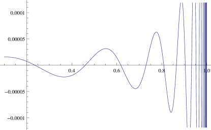
Figure 1. (Color online) Plot of $\Delta_{0}(x)$. As $x$ approaches $1$, with every oscillation, frequency of oscillations of $\Delta_{0}(x)$ increases 2 times, and its amplitude increases 2 times.

Due to such periodicity of $\Delta_{0}(x)$, it is enough to study this function at any interval $[x,(x+1)/2]$ for complete knowledge of the function. The function $\Delta_{0}(x)$ is dominated by the largest ($k=\pm 1$) terms of the sum (2.2), and these two terms add to a function of the form

(2.3) $$\frac{b}{1-x}\cos\left(\log(1-x)\frac{2\pi}{\log 2}+\phi\right).$$

It is sinusoide, which get squeezed horizontally as $x$ approaches $1$, and get stretched vertically.

We can study and write more about the function $\Delta_{0}(x)$ if needed. In the paper by Campbell [3] he refers to an ingenious approach to finding zeroes of a similar oscillating function examined in a study by Mahler [2], which may be applicable for the functions in our current paper.

Of particular interest to us are zeroes of $\Delta_{0}(x)$. The first zero of $\Delta_{0}(x)$ is $x_{0}\approx 0.23628629$. All consecutive zeroes are given by

(2.4) $$x_{n}=1-\frac{1-x_{0}}{2^{n/2}}.$$

2.2. Approximation of $\Delta(x)$ by $\Delta_{0}(x)$.

How well is $\Delta(x)$ approximated by $\Delta_{0}(x)$? Fig. (2) shows the plots of both $\Delta_{0}(x)$ and $\Delta(x)$. At smaller $x$, $\Delta_{0}(x)$ and $\Delta(x)$ differ considerably, but as $x$ approaches $1$, $\Delta_{0}(x)$ and $\Delta(x)$ converge.

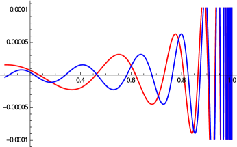
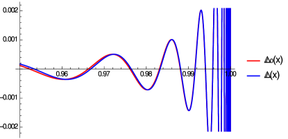
Figure 2. (Color online) Plots of $\Delta_{0}(x)$ and $\Delta(x)$ at intervals [0.2, 1] (left) and [0.95, 1] (right). As $x$ approaches $1$, $\Delta_{0}(x)$ and $\Delta(x)$ converge.

2.2.1. Numerical estimates.

A few first zeroes of $\Delta(x)$ and $\Delta_{0}(x)$, and relative error of approximation, given by $|$((zero of $\Delta(x)$) - (zero of $\Delta_{0}(x)$))/(1 - (zero of $\Delta(x)$))$|$ is shown in Table (1).

zero of $\Delta(x)$	zero of $\Delta_{0}(x)$	relative error
0.4659328665	0.2362862900	0.4299957
0.5827324804	0.4599728568	0.2941988
0.6825927537	0.6181431450	0.2030502
0.7633691635	0.7299864284	0.1410752
0.8261917175	0.8090715725	0.0985002
0.8737099995	0.8649932142	0.0690220
0.9089508885	0.9045357863	0.0484914
0.9347245581	0.9324966071	0.0341315
0.9533891590	0.9522678931	0.0240559
0.9668115422	0.9662483035	0.0169709
0.9764164885	0.9761339466	0.0119805
0.9832657536	0.9831241518	0.0084618
0.9881378894	0.9880669733	0.0059784
0.9915975764	0.9915620759	0.0042250
0.9940512509	0.9940334866	0.0029862
0.9957899259	0.9957810379	0.0021111
0.9970211888	0.9970167433	0.0014924
0.9978927427	0.9978905190	0.0010552
0.9985094836	0.9985083717	0.0007460
0.9989458157	0.9989452595	0.0005276
0.9992544639	0.9992541858	0.0003730
0.9994727689	0.9994726297	0.0002639
0.9996271624	0.9996270929	0.0001865
0.9997363497	0.9997363149	0.0001319
0.9998135638	0.9998135465	0.0000930
0.9998681661	0.9998681574	0.0000663
0.9999067776	0.9999067732	0.0000469
0.9999340809	0.9999340787	0.0000334
0.9999533877	0.9999533866	0.0000236
0.9999670399	0.9999670394	0.0000154
0.9999766936	0.9999766933	0.0000120
0.9999835198	0.9999835197	0.0000071
0.9999883467	0.9999883467	0.0000018

Table 1. Zeroes of $\Delta(x)$ and $\Delta_{0}(x)$.

As $x$ approaches $1$, the relative error goes to zero. The estimate of relative error can be given comparing Taylor series expansion for $\Delta(x)$ and $\Delta_{0}(x)$. If $x_{z}$ is a zero of $\Delta(x)$, and $x_{z0}$ is corresponding zero of $\Delta_{0}(x)$, then

(2.5) $$(1-x_{z0})\approx(1-x_{z})+\frac{1}{2}(1-x_{z})^{2}+\frac{1}{3}(1-x_{z})^{3},$$

or

(2.6) $$(1-x_{z})\approx(1-x_{z0})-\frac{1}{2}(1-x_{z0})^{2}-\frac{1}{3}(1-x_{z0})^{3}.$$

3. Arbitrary $a$

The results of the previous section are applicable to the equation with an arbitrary $a$ instead of $2$. Consider the bilateral infinite series that converges for real $0<x<1$,

$$f(x)=\sum_{n\in Z}a^{n}x^{a^{n}}$$

$$=...+a^{10}x^{a^{10}}+a^{9}x^{a^{9}}+a^{8}x^{a^{8}}+a^{7}x^{a^{7}}+a^{6}x^{a^{6}}+a^{5}x^{a^{5}}+a^{4}x^{a^{4}}$$

$$+a^{3}x^{a^{3}}+a^{2}x^{a^{2}}+ax^{a}+x+\frac{x^{1/a}}{a}+\frac{x^{1/a^{2}}}{a^{2}}+\frac{x^{1/a^{3}}}{a^{3}}+\frac{x^{1/a^{4}}}{a^{4}}$$

$$+\frac{x^{1/a^{5}}}{a^{5}}+\frac{x^{1/a^{6}}}{a^{6}}+\frac{x^{1/a^{7}}}{a^{7}}+\frac{x^{1/a^{8}}}{a^{8}}$$

$$+\frac{x^{1/a^{9}}}{a^{9}}+\frac{x^{1/a^{10}}}{a^{10}}+...$$

Next consider the function given by real $0<x<1$,

(3.2) $$g(x)=\frac{1}{((\log a)\log(1/x))}.$$

(3.3) $$f(x)=g(x)+\Delta(x),$$

where $\Delta(x)$ oscillates around zero, and the amplitude of the oscillations only are noticeable around the third or fourth decimal place. Both $f(x)$ and $g(x)$ satisfy the functional equation $af(x^{2})=f(x)$, and $f(x)=g(x)$ approximately to 3 or 4 decimal places. The $\Delta(x)$ oscillations become “more wriggly” as $x$ approaches $1$ near it’s limiting boundary value of convergence. $\Delta(x)$ is an oscillating periodic function of $\log(\log(1/x))$. The correct formula corresponding to (3.3) is for $|x|<1$,

(3.4) $$\sum a^{k}x^{a^{k}}=\frac{1}{((\log a)(\log(1/x)))}\left\{1-{\sum}^{\prime}\Gamma\left(1+\frac{2ki\pi}{\log a}\right)\left(\log\left(\frac{1}{x}\right)\right)^{-2ki\pi/\log a}\right\},$$

where the sum $\sum$ is over all integers $k$, and the sum $\sum^{\prime}$ is over all nonzero integers $k$.

$\Delta(x)$ may be approximated by

(3.5) $$\Delta_{0}(x)=\frac{1}{\log a}{\sum}^{\prime}\Gamma\left(1+\frac{2ki\pi}{\log 2}\right)(1-x)^{-1-2ki\pi/\log a}$$

As an example, we consider $a=3$. Fig. (3) shows the plots of both $\Delta_{0}(x)$ and $\Delta(x)$. At smaller $x$, $\Delta_{0}(x)$ and $\Delta(x)$ differ considerably, but as $x$ approaches $1$, $\Delta_{0}(x)$ and $\Delta(x)$ converge.

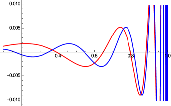
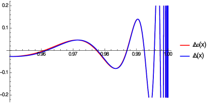
Figure 3. (Color online) Plots of $\Delta_{0}(x)$ and $\Delta(x)$ at intervals [0.2, 1] (left) and [0.95, 1] (right). As $x$ approaches $1$, $\Delta_{0}(x)$ and $\Delta(x)$ converge.

Zeroes of $\Delta(x)$ may be approximated by zeroes of $\Delta_{0}(x)$. The first zero of $\Delta_{0}(x)$ can be found by numerically solving equation $\Delta_{0}(x)=0$. Approximately, taking only the first terms of the sum,

(3.6) $$\Gamma\left(1+\frac{2i\pi}{\log a}\right)(1-x)^{-1-2i\pi/\log a}+\Gamma\left(1-\frac{2i\pi}{\log a}\right)(1-x)^{-1+2i\pi/\log a}=0$$

(3.7) $$x_{0}\approx 1-e^{\frac{\left(\frac{\pi}{2}-arg\left(\Gamma\left(1+\frac{2\pi i}{\log a}\right)\right)\right)\log a}{-2\pi}}$$

All consecutive zeroes are given by

(3.8) $$x_{n}=1-\frac{1-x_{0}}{a^{n/2}}.$$