Large-scale normal fluid circulation in helium superflows

Abstract

We perform fully-coupled numerical simulations of helium II pure superflows in a channel, with vortex-line density typical of experiments. Peculiar to our model is the computation of the back-reaction of the superfluid vortex motion on the normal fluid and the presence of solid boundaries. We recover the uniform vortex-line density experimentally measured employing second sound resonators and we show that pure superflow in helium II is associated with a large-scale circulation of the normal fluid which can be detected using existing particle-tracking visualization techniques.

I Introduction

The problem of velocity profiles in channel flows dates back to the pioneering studies of Poiseuille Poiseuille (1838) and Hagen Hagen (1839). Stimulated by genuine curiosity and industrial purposes, in 1845 Stokes determined that the profile of an incompressible viscous fluid flowing along a channel is parabolicStokes (1845); Sutera and Skalak (1993) (Poiseuille profile). Surprisingly, despite half a century of experiments since the first studies performed by Vinen Vinen (1957a) and current important applications of cryogenics engineering Van Sciver (2012), we still do not know the profile of superfluid helium (helium II) flows in a channel. The difficulty lies in helium II’s nature as the intimate mixture of two fluid components Landau (1941); Donnelly (1991): a viscous normal fluid and a inviscid superfluid. The former can be effectively modelled as an ordinary (classical) fluid obeying the Navier–Stokes equation; the latter is akin to textbooks’ irrotational inviscid Euler fluid. Besides the lack of viscosity, the key property of the superfluid component is that, at speed exceeding a small critical value, the potential flow breaks down, forming a disordered tangle of thin vortex lines of quantized circulation Donnelly (1991); Nemirovskii (2013) (unlike classical fluids whose vorticity is a continuous field). These vortex lines couple normal fluid and superfluid via a mutual friction force which depends nonlinearly on the velocity difference between superfluid and normal fluid and the density of the vortex lines. Barenghi et al. (1983)

The early studies of helium II channel flowsTough (1982) lacked the spatial resolution to determine flow profiles, and focused instead on global properties such as the vortex line density. The development of innovative low-temperature flow visualization techniques (based on micron-sized tracers Zhang and Van Sciver (2005); Bewley et al. (2006) or laser-induced fluorescence Guo et al. (2010)) has renewed the interest in flow profiles. Recent experiments on thermal counterflow (a regime in which superfluid and normal fluid move in opposite directions driven by a small heat flux) have shown that the normal fluid has a tail-flattened laminar profile Marakov et al. (2015) which undergoes a turbulent transition Marakov et al. (2015); Melotte and Barenghi (1998) at larger heat flux.

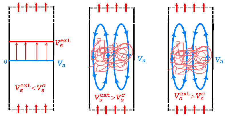
Figure 1: (Color online). Schematic illustration of the normal fluid (blue) and superfluid (red) velocity profiles in a pure superflow channel in a vortex free flow (left). (Middle) and (right): conjectures of normal fluid large flow structures in presence of a vortex tangle.

In this report we focus instead on pure superflow, another interesting regime in which the normal fluid is (on the average) at rest with respect to the channel’s walls, while the net superfluid flow is non-zero. Pure superflow is easily driven thermally or mechanically by blocking a section of the channel with two superleaks. Ashton et al. (1981); Opatowsky and Tough (1981); Baehr et al. (1983); Baehr and Tough (1984); Babuin et al. (2012, 2015a) If the applied superflow $v_{s}^{ext}$ is less than a small critical velocity $v_{s}^{c}$, the system is vortex-free, the normal fluid being quiescent and the superfluid flowing uniformly as schematically shown in Fig. 1 (left). The question which we address Chagovets and Skrbek (2008) is what happens when $v_{s}^{ext}>v_{s}^{c}$ and a turbulent tangle of vortices is formed.

Presumably, the vortices via the mutual friction force locally accelerate the normal fluid in the direction of $v_{s}^{ext}$, giving rise to large-scale normal fluid circulation whose hypothetical features are shown in Fig. 1 (middle) and (right). By numerically simulating the two-fluid flow in a dynamically self-consistent way Galantucci et al. (2015) (which allows the normal fluid to affect the vortex lines motion and viceversa, unlike the traditional approach of Schwarz Schwarz (1988); Baggaley and Laizet (2013); Baggaley and Laurie (2015); Yui and Tsubota (2015); Khomenko et al. (2015)), here we show that the normal fluid’s circulation pattern coincides with the one schematically shown in Fig. 1 (right). The importance of this result stems from the belief that the dynamical state of the normal fluid accounts for the significant observed differences between pure superflow and thermal counterflow. Tough et al. (1981); Babuin et al. (2012); Varga et al. (2015); Babuin et al. (2015a) Finally, we show that our prediction can be easily tested using existing flow visualization based on solid hydrogen and deuterium tracer particles. Bewley et al. (2006); La Mantia et al. (2013); La Mantia and Skrbek (2014)

II Model

We consider an infinite two–dimensional channel of width $D$. Let $x$ and $y$ be respectively the directions along and across the channel with walls at $y=\pm D/2$ and periodic boundary conditions imposed at $x=0$ and $x=L_{x}$. The driving superfluid flow is oriented in the positive $x$ direction.

The superfluid vortices are modelled as $N$ vortex–points of circulation $\Gamma_{j}$ and position $\mathbf{r}_{j}(t)=\left(x_{j}(t),y_{j}(t)\right)$, where $j=1,\cdots N$ and $t$ is time. Half the vortices have positive circulation $\Gamma_{j}=\kappa$ and half have negative circulation $\Gamma_{j}\leavevmode\nobreak\ =\leavevmode\nobreak\ -\kappa$, where $\kappa=10^{-3}\rm cm^{2}/s$ is the quantum of circulation in superfluid ⁴He.

To make connection with experiments we interpret $n=N/(DL_{x})$ (average number of vortex–points per unit area) as the two–dimensional analogue of the three–dimensional vortex–line density $L$, and relate $L$ to the magnitude of the driving superfluid velocity $v_{s}^{ext}$ using past experimental data Ashton et al. (1981); Opatowsky and Tough (1981); Baehr et al. (1983); Baehr and Tough (1984); Babuin et al. (2012) consistent with Vinen’s relation Vinen (1957b) $L^{1/2}=\gamma(v_{s}^{ext}-v_{c})$, where $\gamma$ is a temperature dependent coefficient and $v_{c}$ the critical velocity.

The vortex points move according to Schwarz (1988)

$$\displaystyle\frac{d\mathbf{r}_{j}}{dt} = \mathbf{v}_{s}^{0}(\mathbf{r}_{j},t)+\mathbf{v}_{si}(\mathbf{r}_{j},t)$$ (1)

$$+\alpha\,\mathbf{s}_{j}^{\prime}\times\left(\mathbf{v}_{n}(\mathbf{r}_{j},t)-\mathbf{v}_{s}^{0}(\mathbf{r}_{j},t)-\mathbf{v}_{si}(\mathbf{r}_{j},t)\right)$$

$$+\alpha^{\prime}\left(\mathbf{v}_{n}(\mathbf{r}_{j},t)-\mathbf{v}_{s}^{0}(\mathbf{r}_{j},t)-\mathbf{v}_{si}(\mathbf{r}_{j},t)\right)$$

where $\mathbf{s}_{j}^{\prime}$ is the unit vector along vortex $j$ (in the positive or negative $z$ direction depending on whether $\Gamma_{j}$ is positive or negative), $\alpha$ and $\alpha^{\prime}$ are temperature dependent mutual friction coefficients Barenghi et al. (1983), $\mathbf{v}_{n}(\mathbf{r}_{j},t)$ is the normal fluid velocity at position $\mathbf{r}_{j}$, $\mathbf{v}_{s}^{0}(\mathbf{r}_{j},t)$ is the superfluid flow which enforces the superfluid incompressibility constraint at each channel cross-section and $\mathbf{v}_{si}(\mathbf{r}_{j},t)$ is the superfluid velocity field induced by all the $N$ vortex–points at $\mathbf{r}_{j}$:

$$\mathbf{v}_{si}(\mathbf{r}_{j},t)=\sum_{k=1\dots N}\mathbf{v}_{si,k}(\mathbf{r}_{j},t)\,.$$ (2)

To determine the superfluid velocity field induced by the $k$-th vortex $\mathbf{v}_{si,k}(\mathbf{x},t)$ we employ a complex–potential–based formulation enforcing the boundary condition that, at each wall, the superfluid has zero velocity component in the wall–normal direction Galantucci et al. (2015).

The superfluid velocity $\mathbf{v}_{s}^{0}(\mathbf{x},t)=\left(u_{s}^{0}(x,t),0\right)$ in Eq. (1) is instead obtained by enforcing at each channel cross-section the superfluid flow rate determined by the constant driving superfluid velocity $\mathbf{v}_{s}^{ext}=\left(v_{s}^{ext},0\right)$, i.e

$$\displaystyle u_{s}^{0}(x,t)+\langle u_{si}\rangle(x,t)=v_{s}^{ext}$$ (3)

where $\mathbf{v}_{si}=\left(u_{si},v_{si}\right)$ to ease notation and $\langle\cdot\rangle$ indicates averaging over channel cross-sections.

To model the creation and the destruction of vortices (mechanisms intrinsically three-dimensional) within our two–dimensional model and to mantain a steady state, we employ the “numerical vortex reconnection” procedure described, tested and used in our previous papers Galantucci et al. (2011); Galantucci and Sciacca (2012, 2014); Galantucci et al. (2015): when the distance between two vortex points of opposite circulation becomes smaller than a critical value $\epsilon_{1}$ or when the distance between a vortex point and a boundary is less than $\epsilon_{2}=0.5\epsilon_{1}$, we remove these vortex-points and re-insert them into the channel in a random position. (refer to Ref. [Galantucci et al., 2015] and Supplementary Material for further insight on this numerical reconnection model).

To investigate the dynamical state of the normal fluid in this two-dimensional model, we apply the vorticity-stream function formulation to the incompressible Hall-Vinen-Bekarevich-Khalatnikov (HVBK) equations Landau (1941); Bekarevich and Khalatnikov (1961) obtaining the following set of equations

$$\displaystyle\nabla^{2}\Psi=-\omega_{n}\,\,,$$ (4)

$$\displaystyle\frac{\partial{\omega_{n}}}{\partial{t}}+\frac{\partial{\Psi}}{\partial{y}}\frac{\partial{\omega_{n}}}{\partial{x}} - \frac{\partial{\Psi}}{\partial{x}}\frac{\partial{\omega_{n}}}{\partial{y}}$$

$$=\nu_{n}\nabla^{2}\omega_{n} + \displaystyle\frac{1}{\rho_{n}}\left(\frac{\partial{\widetilde{F}^{y}}}{\partial{x}}-\frac{\partial{\widetilde{F}^{x}}}{\partial{y}}\right)$$ (5)

where $\widetilde{\mathbf{F}}_{ns}=(\widetilde{F}^{x},\widetilde{F}^{y})$ is the mutual friction force and the stream function $\Psi$ and the normal vorticity $\omega_{n}$ are defined as follows: $\displaystyle\mathbf{v}_{n}=\left(\frac{\partial{\Psi}}{\partial{y}},-\frac{\partial{\Psi}}{\partial{x}}\right)$ , $\displaystyle\omega_{n}=\left(\nabla\times\mathbf{v}_{n}\right)\cdot\hat{\mathbf{z}}\,\,$ ($\hat{\mathbf{z}}$ being the unit vector in the $z$ direction).

To model the mutual friction force $\mathbf{F}_{ns}$, we employ the coarse–grained approach of Hall and Vinen Hall and Vinen (1956) according to which, at lengthscales larger than the average inter-vortex spacing $\ell$, the mutual friction assumes the following expression:

$$\widetilde{\mathbf{F}}_{ns}=\alpha\rho_{s}\widehat{\widetilde{\bm{\omega}}}_{s}\times\left[\widetilde{\bm{\omega}}_{s}\times\left(\widetilde{\mathbf{v}}_{n}-\widetilde{\mathbf{v}}_{s}\right)\right]+\alpha^{\prime}\rho_{s}\widetilde{\bm{\omega}}_{s}\times\left(\widetilde{\mathbf{v}}_{n}-\widetilde{\mathbf{v}}_{s}\right)\,\,,$$ (6)

where the symbol $\widetilde{\,}$ over a quantity indicates that this quantity is coarse–grained. At this level of averaging, information about individual vortex lines is lost, hence it is possible to define continuous macroscopic superfluid velocity and vorticity fields, $\widetilde{\mathbf{v}}_{s}$ and $\widetilde{\bm{\omega}}_{s}$ respectively. When computing coarse-grained quantities, we smooth the vortex distribution using a Gaussian kernel to prevent rapid fluctuations of the mutual friction force Galantucci et al. (2015) (cfr. Supplementary Material for a detailed description of the coarse-graining procedure and its smearing effects).

This coarse-grained approach implies to distinguish between the fine $\left(\Delta x,\Delta y\right)$ grid on which the normal fluid velocity $\mathbf{v}_{n}$ is numerically determined, and the coarser $\left(\Delta X,\Delta Y\right)$ grid on which we define the mutual friction $\widetilde{\mathbf{F}}_{ns}$. In principle, we would like to have $\Delta X$ and $\Delta Y\leavevmode\nobreak\ \gg\leavevmode\nobreak\ \ell$ corresponding to the Hall–Vinen limit; in practice, due to computational limitations, we use $\Delta X\,,\,\Delta Y\leavevmode\nobreak\ >\leavevmode\nobreak\ \ell\leavevmode\nobreak\ >\leavevmode\nobreak\ \Delta x\,,\,\Delta y$. Once the mutual friction force $\widetilde{\mathbf{F}}_{ns}$ is computed on the coarse grid we interpolate it on the finer grid via a two–dimensional bi–cubic convolution kernel Keys (1981) whose order of accuracy is between linear interpolation and cubic splines orders of accuracy. It is worth noting that an other method for coupling normal fluid and superfluid motions has also been presented in past studies Idowu et al. (2000a, b); Kivotides (2011), employing a more fine-scale approach, i. e. calculating the mutual friction force exerted by each individual vortex on the normal fluid.

We choose the parameters of the numerical simulations in order to be able to make at least qualitative comparisons with the recent experimental superflow studies performed in Prague Babuin et al. (2012, 2015a); Varga et al. (2015). In particular, we set the width of the numerical channel $D=2.0\,\,\rm mm$ (comparable to the experimental width $D_{\rm exp}=7\div 10\,\,\rm mm$ Babuin et al. (2012, 2015a); Varga et al. (2015)), its length $L_{x}=3D$ and we choose the number of vortices $N$ and the average superfluid driving velocity $v_{s}^{ext}$ to be consistent with second sound measurements reported in Ref. [Babuin et al., 2012]: $N=3072$ and $v_{s}^{ext}=1.25\rm cm/s$, leading to $n^{1/2}D=32$. It is worth noting that the dimensionless quantity $n^{1/2}D$ is a measure of the superfluid turbulent intensity (i.e. the larger $n^{1/2}D$, the more intense the superfluid turbulence) and it is the relevant quantity to be used when comparing different experiments and when drawing parallels between experiments and numerical simulations. The normal fluid being accelerated by the motion of vortices implies that the Reynolds number of the normal fluid flow $\displaystyle Re_{n}<\frac{v_{s}^{ext}(D/2)}{\nu_{n}}=320$, far below the critical Reynolds number for the onset of classical turbulent channel flows $Re_{c}\approx 5772$. Orszag (1971). We reckon therefore that in our numerical experiment the flow of the normal fluid is still laminar.

$\,\,\,\,\,D\,\,\,\,\,$	$2$	$T$	$1.7K$
$L_{x}$	$6$	$\rho_{s}/\rho_{n}$	$3.373$
$N$	$3072$	$\ell$	$6.25\times 10^{-2}$

Table 1: Physical and numerical parameters employed in the simulations in dimensionless units

The complete list of parameters employed in our simulation and the physical relevant quantities are reported in Table 1 and Supplementary Material, expressed in terms of the following units of length, velocity and time, respectively: $\delta_{c}=D/2=1.0\times 10^{-1}\,\rm cm$, $u_{c}=\kappa/(2\pi\delta_{c})=1.59\times 10^{-3}\,\rm cm/s$, $t_{c}=\delta_{c}/u_{c}=62.79\,\rm s$. Hereafter all the quantities which we mention are dimensionless, unless otherwise stated.

For further numerical details concerning the numerical model employed in order to perform the simulations refer to the Supplementary Material Section.

III Results

The aim of our numerical simulations is to determine the normal fluid and superfluid velocity profiles across the channel and the spatial distributions of positive and negative vortices in the statistically steady–state regime which is achieved after a time interval $T_{f}$ comparable to the viscous eddy turnover time $D^{2}/\nu_{n}$. To stress that these distributions and profiles are meant to be coarse–grained over channel stripes of size $\Delta Y$, we use the $\overline{\,\cdot\,}$ symbols. The key feature emerging from the numerical simulations is the coarse-grained profile of the normal fluid velocity $\displaystyle\overline{u}_{n}$ in the steady-state regime, reported in Fig. 2 (left). The computed profile of $\displaystyle\overline{u}_{n}$ shows that the back-reaction of the motion of the superfluid vortices is effectively capable of driving the motion of the normal fluid whose local velocity field may hence be different from zero. We interpret the computed coarse-grained profile of $\displaystyle\overline{u}_{n}$ as the signature of large-scale normal fluid structures similar to the ones described schematically in Fig. 1 (right). It is worth noting that in past experimental studies Chagovets and Skrbek (2008) the existence of these normal fluid large structures has been speculated, even though the normal fluid eddies had opposite vorticity (cfr. Fig. 1 (middle)). The discriminant element determining the symmetry of the normal fluid flow pattern, Fig. 1 (middle) or Fig. 1 (right), is the coarse-grained profile of the streamwise component of the mutual friction force $\overline{F}^{x}$, illustrated in Fig. 2 (right), which is parallel to the driving superfluid velocity $\mathbf{v}_{s}^{ext}$ and stronger in the near-wall region. As a consequence, the normal fluid in proximity of the walls is accelerated in the direction of $\mathbf{v}_{s}^{ext}$, while in the central region the normal flow direction is reversed due to the forced re-circulation of the normal fluid arising from the presence of superleaks and the incompressibilty constraint. It is worth emphasizing that a similar profile of $\overline{F}^{x}$ has been recently computed for thermal counterflow Galantucci et al. (2015).

This dynamical equilibrium achieved between the two components of Helium II via the mutual friction coupling is characterized by the polarization of the superfluid vortex distribution, which is the other key feature arising from the numerical simulations. This spatial configuration of the vortex points can be qualitatively observed in an instantaneous snapshot of the vortex configuration in the steady state (Fig. 3 (left)) and clearly emerges from the coarse-grained positive and negative vortex density profiles illustrated in Fig. 3 (right). To investigate quantitatively the polarization of the vortex distribution, we introduce the coarse–grained polarization vector $\overline{\mathbf{p}}(y)$ defined by Jou et al. (2008)

$$\overline{\mathbf{p}}(y)=\frac{\overline{\bm{\omega}}_{s}(y)}{\kappa\overline{n}(y)}=\frac{\overline{n}^{+}(y)-\overline{n}^{-}(y)}{\overline{n}^{+}(y)+\overline{n}^{-}(y)}\hat{\mathbf{z}}\,,$$ (7)

and plot its magnitude $\overline{p}(y)$ in the inset of Fig. 3 (right). This polarized pattern directly arises from the vortex–points equations of motion (1), where the friction term containing $\alpha$ depends on the polarity of the vortex. The idealized three-dimensional dynamics corresponding to this polarity-dependent vortex-point motion is a streamwise flow of expanding vortex-rings lying on planes perpendicular to $\mathbf{v}_{s}^{ext}$ and drifting in the same direction of the latter. This three-dimensional analogue is very similar to the one recently illustrated for thermal counterflow Galantucci et al. (2015) and consistent with past three-dimensional analytical Nemirovskii and Tsubota (1998) and numerical Schwarz (1988); Baggaley and Laurie (2015); Yui and Tsubota (2015) investigations.

This polarization of the vortex configuration, which, we stress, is not complete, i.e. $|\overline{p}(y)|<1$, generates a parabolic coarse–grained superfluid velocity profile $\overline{u}_{s}(y)\sim y^{2}$ which is reported in Fig. 2 (left) and is similar to the coarse-grained profile computed in recent counterflow simulations Galantucci et al. (2015).

It is important to emphasize that our model, although being two–dimensional, recovers an almost constant profile for the total vortex density $\overline{n}(y)$ across the channel (exception made for the near-wall region, cfr. Fig. 3 (right) ) consistent with the recent experimental measurements performed in Prague Varga et al. (2015).

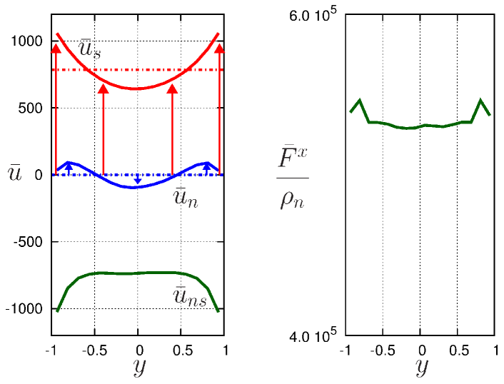
Figure 2: (Color online). (left): coarse–grained profiles of superfluid velocity $\overline{u}_{s}$ (solid red line), normal fluid velocity $\overline{u}_{n}$ (solid blue line) and velocity difference $\overline{u}_{ns}=\overline{u}_{n}-\overline{u}_{s}$ (solid green line) at $t=T_{f}$. Red and blue dot–dashed lines indicate the initial laminar velocity profiles of the superfluid and the normal fluid, respectively; (right): coarse–grained profile of the streamwise component of the mutual friction force $\overline{F}^{x}/\rho_{n}\,$ at $t=T_{f}$.

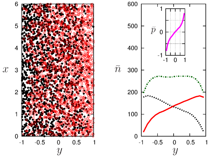
Figure 3: (Color online). (left): vortex distribution at $t=T_{f}$, red empty (black filled) circles indicate positive (negative) vortices; (right): coarse–grained profiles of positive vortex density $\overline{n}^{+}$ (solid red line), negative vortex density $\overline{n}^{-}$ (dashed black line) and total vortex density $\overline{n}$ (dot–dashed green line) at $t=T_{f}$. In the inset, we report the corresponding coarse–grained profile of the polarization magnitude $\overline{p}$ (solid magenta line).

IV Conclusions

In conclusion, we have performed self-consistent numerical simulations of the coupled normal fluid-superfluid motion in a pure superflow channel, with values of the vortex-line density typical of recent experiments Babuin et al. (2012). The main features of our model are that it is dynamically self-consistent (the normal fluid affects the superfluid and viceversa) unlike the traditional approach of Schwarz, and that it takes into account the presence of channel’s boundaries. The main approximation of our model is that it is two-dimensional (as in many studies of classical channel flows). Nevertheless, we think that this model captures the essential physical features of the superflow problem: firstly, the model worked well when applied to counterflow experiments Galantucci et al. (2015); Marakov et al. (2015); secondly, in the superflow problem, it predicts the observed almost constant vortex density profile Varga et al. (2015).

Our main prediction is that the normal fluid executes a large-scale circulation - see Fig. 1 (right). The prediction can be tested experimentally employing Particle-Tracking-Velocimetry Visualization techniques Bewley et al. (2006); La Mantia et al. (2013); La Mantia and Skrbek (2014). We know Poole et al. (2005) that at any instant a tracer particle is either free (in which case it is dragged along by the normal fluid) or trapped in a vortex line (which, in first approximation, moves with the applied superflow). Therefore, in near-wall regions of the channel we should observe that all particles move in the same direction, whereas the central region of the channel should contain particles moving in both directions. The effect is schematically shown in Fig. 4.

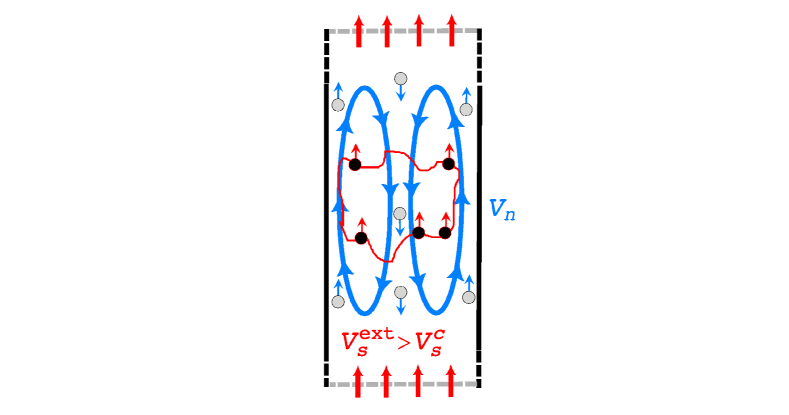
Figure 4: (Color online). As in Fig. 1 (right) but with tracer particles, which are either free (light-grey circles) or trapped in vortices (black circles).

Experimental verification of this effect should strengthen our general understanding of superfluid hydrodynamics and of the dynamics of tracer particles in helium II. It should also open the way for a better understanding of the onset, steady-state and decaying state of quantum turbulence. Tough et al. (1981); Babuin et al. (2015a)