Virtual Element Method for Second Order Elliptic Eigenvalue Problems

Abstract

We study the virtual element (VEM) approximation of elliptic eigenvalue problems. The main result of the paper states that VEM provides an optimal order approximation of the eigenmodes. A wide set of numerical tests confirm the theoretical analysis.

1 Introduction

The Virtual Element Method (VEM) is a brand new approximation technique introduced in [8] which has been applied to several problems. In its abstract formulation the method is a generalization of the conforming finite element method which allows, nevertheless, the use of general polygonal and polyhedral meshes without having to integrate complex non-polynomial functions on the elements.

The Virtual Element Method has been developed successfully for a large range of problems: the linear elasticity problems, both for the compressible and the nearly incompressible case [9, 34], a stream and a non-conforming formulation of VEMs for the Stokes problem [3, 30], the non-linear elastic and inelastic deformation problems, mainly focusing on a small deformation regime [17], the Darcy problem in mixed form [26], the plate bending problem [27], the Steklov eigenvalue problem [36], the general second order elliptic problems in primal [14] and mixed form [11], the Cahn-Hilliard equation [4], the Helmholtz problem [39], the discrete fracture network simulations [22, 21], the time-dependent diffusion problems [42, 41] and the Stokes problem [18]. In [5, 29] the authors present a non-conforming Virtual Element Space. A posteriori error estimates are studied in [20, 28, 37]. $H(div)$ and $H(curl)$ VEM and VEM with arbitrary regularity are presented in [7] and [19], respectively. In [15] the VEM $hp$ version is analyzed. Finally, in [13, 12] the authors introduce the last version of Virtual Element spaces, the Serendipity VEM spaces that, in analogy with the Serendipity FEMs, allows to reduce the number of degrees of freedom.

In this paper we study the Virtual Element Method applied to elliptic eigenvalue problems. As a model problem we consider the Laplace eigenvalue problem. Nevertheless the analysis generalizes straightforward to the case of more general second order elliptic eigenvalue problems. The discretization of the problem requires the introduction of two discrete bilinear forms, one being the approximated grad-grad form and the other being a discrete version of the $L^{2}$–inner product. The latter one is built using the techniques of [2]. In particular, we consider both a non-stabilized form and a stabilized one, and we study the convergence properties of the corresponding discrete formulations. It is shown that the Virtual Element Method provides optimal convergence rates both for the eigenfunctions and the eigenvalues.
The paper is organized as follows. In Section 2, we set up the model eigenproblem, while in Section 3 we recall the definition of the bi-dimensional and three-dimensional Virtual Element Spaces. In Section 4 we introduce the virtual element formulation of the problem, and in Section 5 we recall some fundamental results for the spectral approximation of compact operators. In Section 6 we prove the main results of the paper, which consist in the a optimal priori error estimates for the VEM approximation of general elliptic eigenvalue problems. We discuss the implementation details in Section 7 and show the behaviour of the method for a set of numerical examples. We finally draw the conclusions in Section 8.

2 Setting of the problem

We are interested in the problem of computing the eigenvalues of the Laplace operator, namely
find $\lambda\in\mathbb{R}$ such that there exists $u$, with $\|u\|_{0}=1$ satisfying

$$\left\{\begin{array}[]{ll}-\Delta u=\lambda u&\text{in }\Omega\\ u=0&\text{on }\Gamma,\end{array}\right.$$ (1)

where $\Omega\subset\mathbb{R}^{n}\ (n=2,3)$ is a bounded polygonal/polyhedral domain with Lipschitz boundary $\Gamma$.

For ease of exposition, we focus on the case of Dirichlet boundary conditions. The extension to other boundary conditions are analogous.

The variational formulation of problem (1) reads:
find $\lambda\in\mathbb{R}$ such that there exists $u\in V$, with $\|u\|_{0}=1$ satisfying

$$a(u,v)=\lambda b(u,v)\quad\forall v\in V,$$ (2)

where $V=H^{1}_{0}(\Omega)$, $a(u,v)=\int_{\Omega}\nabla u\cdot\nabla v$, and $b(\cdot,\cdot)$ denotes the $L^{2}$-inner product.
It is well-know that the eigenvalues of problem (2) form a positive increasing divergent sequence, and that the corresponding eigenfunctions are an orthonormal basis of $V$ with respect both to the $L^{2}$-inner product and to the scalar product associated with the bilinear form $a(\cdot,\cdot)$.
Due to regularity results [1], there exists a constant $r>1/2$ depending on $\Omega$, such that the solution $u$ belongs to the space $H^{1+r}(\Omega)$. It can be proved that $r$ is at least one if $\Omega$ is a convex domain, while $r$ is at least $\pi/\omega-\varepsilon$ for any $\varepsilon>0$ for a non–convex domain, being $\omega<2\pi$ the maximum interior angle of $\Omega$.

We will also need the source problem associated with the eigenvalue problem (2): given $f\in L^{2}(\Omega)$, find $u^{s}\in V$ such that

$$a(u^{s},v)=b(f,v)\quad\forall v\in V.$$ (3)

Throughout the paper, we will make use of the following notation. We will denote by $|\cdot|_{s,\omega}$ and $\|\cdot\|_{s,\omega}$ the seminorm and the norm in the Sobolev space $H^{s}(\omega)$, respectively, while $(\cdot,\cdot)_{\omega}$ will denote le $L^{2}$-inner product over the domain $\omega$. Moreover, if $\omega=\Omega$, the subscript $\omega$ may be omitted. For a positive integer $k$, $\mathbb{P}_{k}(\omega)$ will denote the space of polynomials on $\omega$ of degree at most $k$. Finally, $a^{\omega}(\cdot,\cdot)$ and $b^{\omega}(\cdot,\cdot)$ will denote respectively the restriction of the form $a(\cdot,\cdot)$ and $b(\cdot,\cdot)$ on $\omega$.

3 Virtual Element Spaces

In this section, we briefly recall the definition of the Virtual Element Spaces. We present separately the the bi-dimensional and the three-dimensional case.

3.1 Bi-dimensional case

Let $\{\mathcal{T}_{h}\}_{h}$ be a sequence of decompositions of $\Omega$ into polygons $P$, and let $\mathcal{E}_{h}$ denote the set of edges $e$ of $\mathcal{T}_{h}$. For every element $P$, we denote by $|P|$ its area and by $h_{P}$ its diameter. Similarly, for each edge $e$, $|e|$ or, equivalentely, $h_{e}$ will denote its length. Depending on the context, $\partial P$ may denote the boundary of element $P$ or the set of the element edges. As usual, the mesh size $h$ is the maximum diameter of the elements $P$ in $\mathcal{T}_{h}$.
In accordance with [8], we assume the following mesh regularity condition: there exist a positive constant $\gamma$, independent of $h$, such that each element $P\in\mathcal{T}_{h}$ is star-shaped with respect to a ball of radius greater than $\gamma h_{P}$, and for every element $P$, and for every edge $e\subset\partial P$, $h_{e}\geq\gamma h_{P}$.

Following [8, 2], for every integer $k\geq 1$ and for every element $P\in\mathcal{T}_{h}$ we define

$$\tilde{V}_{h}^{k}(P):=\{v\in C^{0}(\partial P):v|_{e}\in\mathbb{P}_{k}(e)\ \forall e\subset\partial P,\Delta v\in\mathbb{P}_{k}(P)\}.$$

For each $v$ in $\tilde{V}_{h}^{k}(P)$, we consider the following linear operators $\mathbf{D^{2D}}$ split into three sets:

• $\mathbf{D_{1}^{2D}}$: the values $v(V_{i})$ at the vertices $V_{i}$ of $P$,

• $\mathbf{D_{2}^{2D}}$: the scaled edge moments up to order $k-2$

  $$\dfrac{1}{|e|}\displaystyle{\int_{e}}v\,m\,\text{d}s,\quad\forall m\in\mathcal{M}_{k-2}(e),\quad\text{on each edge $e$ of $P$,}$$

• $\mathbf{D_{3}^{2D}}$: the scaled element moments up to order $k-2$

  $$\dfrac{1}{|P|}\displaystyle{\int_{P}}v\,m\,\text{d}\mathbf{x},\quad\forall m\in\mathcal{M}_{k-2}(P),$$

  
  

where $\mathcal{M}_{k-2}(\omega)$ denotes the set of scaled monomials on $\omega$

$$\mathcal{M}_{k-2}(\omega)=\Big{\{}\Big{(}\dfrac{\mathbf{x}-\mathbf{x}_{\omega}}{h_{\omega}}\Big{)}^{\mathbf{s}},|\mathbf{s}|\leq k-2\Big{\}}$$

being $\mathbf{x}_{\omega}$ the barycenter of $\omega$, and where we set $\mathcal{M}_{-1}(\omega)=\emptyset$.

Remark 3.1.

It can be proved that each scaled monomial in $\mathcal{M}_{k}(\omega)$, and also the linear operators $\mathbf{D^{2D}}$, scales like $1$ (cf. [10] Remark 1.1., and Remark 2.5.)

Remark 3.2.

The linear operators $\mathbf{D_{3}^{2D}}$ allows to exactly compute the $L^{2}(P)$-projection of any function in $\tilde{V}_{h}^{k}(P)$ onto the local space of piecewise polynomial of degrees at most $k-2$. Indeed, given a function $v\in\tilde{V}_{h}^{k}(P)$, the $L^{2}(P)$-projection of $v$ is defined as the unique element $\Pi^{P}_{k-2}v\in\mathbb{P}_{k-2}(P)$ such that

$$\int_{P}(\Pi_{k-2}^{P}v)\,p\,\text{d}\mathbf{x}=\int_{P}v\,p\,\text{d}\mathbf{x}\quad\text{forall }p\in\mathcal{M}_{k-2}(P).$$ (4)

Notice that  (4) is a linear system with right hand side given by the $\mathbf{D_{3}^{2D}}(v)$.

We observe that, instead, the linear operators $\mathbf{D_{3}^{2D}}$ are not enough to compute the projection onto the space of piecewise polynomial of degree $k$ .

From the linear operators $\mathbf{D^{2D}}$, on each element $P$ we can construct and exactly compute a projection operator $\Pi_{k}^{\nabla}:\tilde{V}_{h}^{k}(P)\rightarrow\mathbb{P}_{k}(P)$ defined as follows:

$$a^{P}(\Pi_{k}^{\nabla}v-v,p)=0\quad\forall p\in\mathbb{P}_{k}(P)$$ (5)

and

$$\int_{\partial P}(\Pi_{k}^{\nabla}v-v)\text{d}s=0\quad\text{for }k=1$$ (6)

or

$$\int_{P}(\Pi^{\nabla}_{k}v-v)\text{d}\mathbf{x}=0\quad\text{for }k\geq 2.$$ (7)

We observe that this operator is well-defined also for functions in $H^{1}(P)$, but in this case it is not exactly computable. On the other hand, for all $v\in\tilde{V}_{h}^{k}$, $\Pi_{k}^{\nabla}v$ can be computed only in terms of $\mathbf{D^{2D}}(v)$.

The local virtual space is then defined as

$$V_{h}^{k}(P):=\Big{\{}v\in\tilde{V}_{h}^{k}(P):\int_{P}v\,p\,\text{d}{\bf{x}}=\int_{P}(\Pi_{k}^{\nabla}v)p\,\text{d}{\bf{x}}\ \forall p\in(\mathbb{P}_{k}/\mathbb{P}_{k-2}(P))\Big{\}},$$ (8)

where $(\mathbb{P}_{k}/\mathbb{P}_{k-2}(P))$ denotes the space of polynomials in $\mathbb{P}_{k}(P)$ $L^{2}$–orthogonal to all polynomials in $\mathbb{P}_{k-2}(P)$.
We recall that, by construction, the local space $V_{h}^{k}(P)$ enjoys the following fundamental properties (see [2]):

• $\mathbf{(P1)}$ the space $\mathbb{P}_{k}(P)\subset V_{h}^{k}(P)$. This property will guarantee the optimal order of approximation

• $\mathbf{(P2)}$ the set of linear operators $\mathbf{D^{2D}}$ constitute a set of degrees of freedom (DoFs) for the space $V_{h}^{k}(P)$

• $\mathbf{(P3)}$ since $V_{h}^{k}(P)\subset\tilde{V}_{h}^{k}(P)$, the operator $\Pi_{k}^{\nabla}$ is well-defined on $V_{h}^{k}(P)$ and it is still computable in terms of the degrees of freedom

• $\mathbf{(P4)}$ the standard $L^{2}$-projection operator $\Pi^{0}_{k}:V_{h}^{k}(P)\rightarrow\mathbb{P}_{k}(P)$ is computable only in terms of the degrees of freedom

• $\mathbf{(P5)}$ for all $v\in V_{h}^{k}(P)$ the vectorvalued function $\Pi^{0}_{k-1}\nabla v_{h}$ can be explicitly computed from the degrees of freedom, see [14].

The global bi-dimensional discrete space is hence defined in the finite element way as

$$V_{h}^{k,2\rm{D}}=\{v\in V:v|{{}_{P}}\in V_{h}^{k}(P)\quad\forall P\in\mathcal{T}_{h}\}.$$

3.2 Three-dimensional case

The aim of this section is to briefly present the extension of the Virtual Element spaces to the three-dimensional case, recalling from [2] the core idea of the three-dimensional VEM.

Let $\{\mathcal{T}_{h}\}_{h}$ be a sequence of decompositions of $\Omega$ into general polyhedral elements $P$. We assume that for all $h$, each element $P\in\mathcal{T}_{h}$ fulfils the following assumptions: there exists a uniform positive constant $\gamma$ such that $P$ is star-shaped with respect to a sphere of radius greater than $\gamma\,h_{P}$, and every face $f$ of $P$ is star-shaped with respect to a ball of radius greater than $\gamma\,h_{f}$, and for every face $f$ of $P$ and for every edge $e$ of $f$, it holds that $h_{e}\geq\gamma\,h_{f}\geq\gamma^{2}\,h_{P}$, where $h_{f}$ (resp. $h_{e}$) denotes the diameter of the face $f$ (resp. the length of the edge $e$).

Let $P$ in $\mathcal{T}_{h}$. We start by defining the virtual local-boundary space, observing that each face $f\in\partial P$ is a polygon. Let us define the following space

$$\mathcal{B}_{h}^{k}(\partial P):=\{v\in C^{0}(\partial P):v|_{f}\in V_{h}^{k,\rm{2D}}(f)\ \forall f\subset\partial P\}.$$ (9)

The above space is made of functions that on each face are two-dimensional virtual functions, that glue continuously across edges. Once the boundary space is defined, the steps to follow in order to define the local virtual space on $P$ become very similar to the two dimensional case. We first introduce a preliminary local virtual element space on $P$

$$\tilde{V}_{h}^{k}(P):=\{v\in H^{1}(P):v|_{\partial P}\in\mathcal{B}_{h}^{k}(\partial P)\ ,\Delta v\in\mathbb{P}_{k}(P)\}.$$

Therefore, extending to the polyhedra the definition $\eqref{eq:virtual2d}$, we can define the local virtual space

$$V_{h}^{k}(P):=\Big{\{}v\in\tilde{V}_{h}^{k}(P):\int_{P}v\,p\,\text{d}{\bf{x}}=\int_{P}(\Pi_{k}^{\nabla}v)p\,\text{d}{\bf{x}}\ \forall p\in(\mathbb{P}_{k}/\mathbb{P}_{k-2}(P))\Big{\}},$$ (10)

Now the degrees of freedom for the space $V_{h}^{k}(P)$ are the obvious three-dimensional counterpart of the DoFs of the bi-dimensional case. Let us define the linear operators $\mathbf{D^{3D}}$ split into three sets:

• $\mathbf{D_{1}^{3D}}$: the values $v(V_{i})$ at the vertices $V_{i}$ of $P$,

• $\mathbf{D_{2}^{3D}}$: the scaled edge moments up to order $k-2$

  $$\dfrac{1}{|e|}\displaystyle{\int_{e}}v\,m\,\text{d}s,\quad\forall m\in\mathcal{M}_{k-2}(e),\quad\text{on each edge $e$ of $\partial P$,}$$

• $\mathbf{D_{3}^{3D}}$: the scaled face moments up to order $k-2$

  $$\dfrac{1}{|f|}\displaystyle{\int_{f}}v\,m\,\text{d}\mathbf{x},\quad\forall m\in\mathcal{M}_{k-2}(f),\quad\text{on each face $f$ of $\partial P$,}$$

• $\mathbf{D_{4}^{3D}}$: the scaled element moments up to order $k-2$

  $$\dfrac{1}{|P|}\displaystyle{\int_{K}}v\,m\,\text{d}\mathbf{x},\quad\forall m\in\mathcal{M}_{k-2}(P).$$

From [2] we have that the three-dimensional space $V_{h}^{k}(P)$ matches the three-dimensional counterpart of the properties $(\mathbf{P1})$, $(\mathbf{P2})$, $(\mathbf{P3})$, $(\mathbf{P4})$, $(\mathbf{P5})$.

Finally, the three-dimensional global virtual space $V_{h}^{k,\rm{3D}}$ is defined by using a standard assembly procedure as in finite elements

$$V_{h}^{k,3\rm{D}}=\{v\in V:v|{{}_{P}}\in V_{h}^{k}(P)\quad\forall P\in\mathcal{T}_{h}\}.$$

4 Virtual Element discretization

This section is devoted to the virtual element discretization of the source and the eigenvalue problem. We underline that the analysis holds both in the two dimensional and the three dimensional case. Therefore, from now on, we do not make any distinction between the spaces in two and three dimensions, and we simply denote by $V_{h}^{k}$ the global VEM space of order $k$.

The Virtual Element discretization of source problem (3) reads

$$\begin{cases}\text{find }u_{h}^{s}\in V_{h}^{k}\text{ such that}\\ a_{h}(u_{h}^{s},v_{h})=\langle f_{h},v_{h}\rangle\quad\forall v_{h}\in V_{h}^{k},\\ \end{cases}$$ (11)

where $\langle\cdot,\cdot\rangle$ denotes the duality pairing in $V_{h}^{k}$, and $f_{h}\in(V_{h}^{k})^{\prime}$. In particular,

$$\langle f_{h},v_{h}\rangle=\sum_{P\in\mathcal{T}_{h}}(\Pi^{0}_{k}f,v_{h})_{P}.$$

The discrete bilinear form $a_{h}(\cdot,\cdot)$ splits as

$$a_{h}(u_{h},v_{h})=\displaystyle{\sum_{P\in\mathcal{T}_{h}}}a_{h}^{P}(u_{h},v_{h}).$$ (12)

with

$$a_{h}^{P}(u_{h},v_{h})=a^{P}(\Pi_{k}^{\nabla}u_{h},\Pi^{\nabla}_{k}v_{h})+S^{P}\Big{(}(I-\Pi_{k}^{\nabla})u_{h},(I-\Pi_{k}^{\nabla})v_{h}\Big{)}.$$ (13)

where $S^{P}(\cdot,\cdot)$ denotes any symmetric positive definite bilinear form on the element $P$ such that there exist two uniform positive constants $c_{0}$ and $c_{1}$ such that

$$c_{0}a^{P}(v,v)\leq S^{P}(v,v)\leq c_{1}a^{P}(v,v)\quad\forall v\in V_{h}^{k}(P){\text{ with }}\Pi^{\nabla}_{k}v=0.$$

Remark 4.1.

The above requirement means that the form $S^{P}(\cdot,\cdot)$ scales as $a^{P}(\cdot,\cdot)$, namely $S^{P}(\cdot,\cdot)\simeq h_{P}^{n-2}$, with $n=2$ in the bi-dimensional case and $n=3$ in the three-dimensional one.

The choice of the discrete form $a_{h}(\cdot,\cdot)$ is driven by the need to satisfy the k-consistency and $stability$ properties, $i.e.$

• $k$-consistency: for all $v\in V_{h}^{k}$ and for all $p\in\mathbb{P}_{k}(P)$ it holds

  $$a_{h}^{P}(v,p)=a^{P}(v,p)$$

• stability: there exists two positive constants $\alpha_{*},\ \alpha^{*}$, independent of $h$ and of $P$, such that

  $$\alpha_{*}a^{P}(v,v)\leq a_{h}^{P}(v,v)\leq\alpha^{*}a^{P}(v,v)\quad\forall v\in V_{h}^{k}.$$

In particular, the first term in (13) ensures $k$–$consistency$, while the second one stability.

The following interpolation and approximation properties hold [28, 25].

Theorem 4.1.

There exists a constant $C$, depending only on the polynomial degree $k$ and the shape regurality $\gamma$, such that for every $s$ with $2\leq s\leq k+1$, for every $h$, for all $P\in\mathcal{T}_{h}$, and for every $w\in H^{s}(\Omega)$ there exists a $w_{I}\in V_{h}^{k}$ such that

$$\|w-w_{I}\|_{0,P}+h_{P}|w-w_{I}|_{1,P}\leq Ch_{P}^{s}|w|_{s,P}.$$ (14)

Theorem 4.2.

There exists a constant $C$, depending only on the polynomial degree $k$ and the shape regurality $\gamma$, such that for every $s$ with $1\leq s\leq k+1$ and for every $w\in H^{s}(\Omega)$ there exists a $w_{\pi}\in\mathbb{P}_{k}(P)$ such that

$$\|w-w_{\pi}\|_{0,P}+h_{P}|w-w_{\pi}|_{1,P}\leq Ch_{P}^{s}|w|_{s,P}.$$ (15)

In [2] it has been proved that the discrete problem (11) is well-posed and that the following optimal a priori error estimate holds.

Theorem 4.3.

Let $u$ be the solution of problem (3) and $u_{h}\in V_{h}^{k}$ be the solution of the discrete problem (11), then for every approximation $u_{I}\in V_{h}^{k}$ of u and for every approximation $u_{\pi}$ of u that is piecewise in $\mathbb{P}_{k}$ it holds

$$|u-u_{h}|_{1}\leq C(|u-u_{I}|_{1}+|u-u_{\pi}|_{1,h}+\mathcal{F}_{h}),$$ (16)

where $C$ is a positive constant depending only on $\alpha_{*}$ and $\alpha^{*}$, and for every h, $\mathcal{F}_{h}(\equiv\|f-f_{h}\|_{V^{\prime}_{h}})$ is the smallest constant such that

$$b(f,v_{h})-<f_{h},v_{h}>\leq\mathcal{F}_{h}|v_{h}|_{1}\quad\forall v_{h}\in V_{h}^{k}.$$

Remark 4.2.

We observe that the same result holds also for general linear second order elliptic problems, provided the form $a(\cdot,\cdot)$ is choosen as in  (33). We refer to [14] for an exaustive analysis.

Remark 4.3.

The interpolation and the approximation estimates in Theorems 4.1 and 4.2, the definition of $<f_{h},v>$, and the stability of the continuous source problem yield that, for $f\in L^{2}(\Omega)$, the a priori error estimate in Theorem 4.3 becomes

$$|u-u_{h}|_{1}\leq C(h^{t}|u|_{1+t}+h\|f\|_{0})\leq Ch^{t}\|f||_{0},$$ (17)

where $t=\min\{k,r\}$, being $k$ the polynomial degree and $r$ the regularity index of the solution $u$.

We are now ready to write the VEM approximation of problem (2):
find $\lambda_{h}\in\mathbb{R}$ such that there exists $u_{h}\in V_{h}^{k}$, with $\|u_{h}\|_{0}=1$ satisfying

$$a_{h}(u_{h},v_{h})=\lambda_{h}b_{h}(u_{h},v_{h})\quad\forall v_{h}\in V_{h}^{k},$$ (18)

where $b_{h}(\cdot,\cdot)=\sum_{P\in\mathcal{T}_{h}}b_{h}^{P}(\cdot,\cdot)$ is a symmetric bilinear forms defined on $V_{h}^{k}\times V_{h}^{k}$.
Two possible choices for the discrete form $b_{h}(\cdot,\cdot)$ are available. The first one is inspired by the virtual approximation of the load term in the source problem (11) and reads as follows:

$$b_{h}^{P}(u_{h},v_{h})=\int_{P}\Pi^{0}_{k}u_{h}\Pi^{0}_{k}v_{h}\,\text{d}\mathbf{x}.$$ (19)

The second possible choice consists in considering a discrete bilinear form $\tilde{b}_{h}(\cdot,\cdot)$ which enjoys not only the $k$–$consistency$ property, but also the $stability$ one. In this case, as done for the discrete form $a_{h}(\cdot,\cdot)$, we define

$$\tilde{b}_{h}^{P}(u_{h},v_{h})=\int_{P}\Pi^{0}_{k}u_{h}\Pi^{0}_{k}v_{h}\,\text{d}\mathbf{x}+\tilde{S}^{P}\Big{(}(I-\Pi_{k}^{0})u_{h},(I-\Pi_{k}^{0})v_{h}\Big{)},$$ (20)

where $\tilde{S}^{P}$ is any positive definite bilinear form on the element $P$ such that there exist two uniform positive constants $\tilde{c}_{0}$ and $\tilde{c}_{1}$ such that

$$\tilde{c}_{0}\,b^{P}(v,v)\leq\tilde{S}^{P}(v,v)\leq\tilde{c}_{1}\,b^{P}(v,v)\quad\forall v\in V_{h}^{k}(P)\text{ with }\Pi_{k}^{0}v=0.$$

Remark 4.4.

In analogy with the condition on the form $S^{P}(\cdot,\cdot)$, we require that the form $\tilde{S}^{P}(\cdot,\cdot)$ scales like $b^{P}(\cdot,\cdot)$, that is $\tilde{S}^{P}(\cdot,\cdot)\simeq h^{n}$, with $n=2$, and $n=3$ in the bi-dimensional and in the three-dimensional case, respectively.

Remark 4.5.

In the definition of the discrete bilinear forms $b_{h}(\cdot,\cdot)$ and $\tilde{b}_{h}(\cdot,\cdot)$, we project onto the space $\mathbb{P}_{k}(P)$ since it has been numerically observed that this gives more accurate results. For sure, this choice does not provide a better convergence rate, due to the k-consistency property.

The second VEM approximation of problem  (2) then reads as
find $\tilde{\lambda}_{h}\in\mathbb{R}$ such that there exists $\tilde{u}_{h}\in V_{h}^{k}$, with $\|\tilde{u}_{h}\|_{0}=1$ satisfying

$$a_{h}(\tilde{u}_{h},v_{h})=\tilde{\lambda}_{h}\tilde{b}_{h}(\tilde{u}_{h},v_{h})\quad\forall v_{h}\in V_{h}^{k}.$$ (21)

In what follows, we will also need the discrete source problem corresponding to the second discrete formulation  (21), which reads as:

$$\begin{cases}\text{find }\tilde{u}_{h}^{s}\in V_{h}^{k}\text{ such that}:\\ a_{h}(\tilde{u}_{h}^{s},v_{h})=\tilde{b}_{h}(f,v_{h})\quad\forall v_{h}\in V_{h}^{k}.\\ \end{cases}$$ (22)

The well–posedness of the discrete formulation  (22) stems from that of the discrete formulation  (11), since the bilinear form $a_{h}(\cdot,\cdot)$ is coercive (due to the stability property).

Summarizing, we consider two different discrete approximation of problems  (2) and  (3), with at the right hand side a non–stabilized bilinear form and a stablized one, respectively.

5 Spectral approximation for compact operators

In this section, we briefly recall some spectral approximation results that can be deduced from [6, 23, 35]. For more general results, we refer to the original papers.

Before stating the spectral approximation results, we introduce a natural compact operator associated with problem (2) and its discrete counterpart and we recall their connection with the eigenmode convergence.

Let $T\in\mathcal{L}(L^{2}(\Omega))$ be the solution operator associated with problem (2), namely $T:L^{2}(\Omega)\rightarrow L^{2}(\Omega)$ is defined by

$$\left\{\begin{array}[]{l}Tf\in V{\text{ such that}}\\ a(Tf,v)=b(f,v)\quad\forall v\in V.\end{array}\right.$$

Operator $T$ is self-adjoint and positive definite. Moreover, operator $T$ is also compact due to the compact embedding of $H^{1}(\Omega)$ into $L^{2}(\Omega)$.

Similarly, let $T_{h}\in\mathcal{L}(L^{2}(\Omega))$ be the discrete solution operator associated with problem (11) defined as

$$\left\{\begin{array}[]{l}T_{h}f\in V{\text{ such that}}\\ a_{h}(T_{h}f,v_{h})=b_{h}(f_{h},v_{h})\quad\forall v_{h}\in V_{h}^{k}.\end{array}\right.$$

Analougosly, the discrete solution operator $\tilde{T}_{h}\in\mathcal{L}(L^{2}(\Omega))$ associated with problem (22) is defined as

$$\left\{\begin{array}[]{l}\tilde{T}_{h}f\in V{\text{ such that}}\\ a_{h}(\tilde{T}_{h}f,v_{h})=\tilde{b}_{h}(f,v_{h})\quad\forall v_{h}\in V_{h}^{k}.\end{array}\right.$$

Operators $T_{h}$ and $\tilde{T}_{h}$ are self-adjoint and compact since their ranges are finite dimensional.
Finally, the eigensolutions of the continuous and the discrete problems (2) and (18) are respectively related to the eigenmodes of operators $T$ and $T_{h}$ in the sense that the corresponding eigenvalues are inverse of each other and their eigenspaces coincide. By virtue of this correspondence, the convergence analysis can be derived from the spectral approximation theory for compact operators.
Since similar considerations hold for the eigenmodes of operators $T$ and $\tilde{T}_{h}$, in the following we present only the results relative to operators $T$ and $T_{h}$.

A sufficient condition for the correct spectral approximation of a compact operator $T$ is the uniform convergence to $T$ of the family of discrete operators $\{T_{h}\}_{h}$ [6, 23]:

$$\|T-T_{h}\|_{\mathcal{L}(L^{2}(\Omega))}\to 0,\quad\text{as }h\to 0,$$ (23)

or, equivalentely,

$$\|Tf-T_{h}f\|_{0}\leq C\rho(h)\|f\|_{0}\quad\forall f\in L^{2}(\Omega),$$ (24)

with $\rho(h)$ tending to zero as $h$ goes to zero.

We remark that  (23), besides the convergence of the eigenmodes, contains also the information that no spurious eigenvalues pollute the spectrum. In fact,

1. each continuous eigenvalue is approximated by a number of discrete eigenvalues (counted with their multiplicity) that corresponds exactly to its multiplicity;

2. each discrete eigenvalue approximates a continuous eigenvalue.

Since operator $T$ is compact and self-adjoint, condition (23) is also necessary for the correct spectral approximation; see [24]. Regarding the rate of convergence of eigenvalues and eigenvectors, we refer to [32, 33].

A simple way to estimate the norm of the difference $T-T_{h}$ is to use a priori error estimates.

6 Convergence analysis of the method

In this section we study the convergence of the discrete eigenmodes provided by the VEM approximation to the continuous ones. We will consider the non–stabilized discrete formulation  (18) and the stabilized one  (21) separately.

6.1 Convergence analysis for the first formulation

In the case of the first VEM approximation of problem  (2), which corresponds to the choice of a non–stabilized $b_{h}(\cdot,\cdot)$ form, the uniform convergence of the sequence of operators ${T_{h}}$ to $T$ directly stems from the a priori error estimates in Remark  (4.3). The optimal rate of convergence of the eigenfunctions and the double rate of convergence of the eigenvalues can then be proved following the arguments in [38], Sections 4.

The following theorem ensures the convergence of eigenmodes.

Theorem 6.1.

The family of operators $T_{h}$ associated with problem  (11) converges uniformly to the operator $T$ associated with problem  (3), that is,

$$\|T-T_{h}\|_{\mathcal{L}(L^{2}(\Omega))}\to 0\ for\ h\to 0.$$ (25)

Let $\lambda$ be an eigenvalue of problem  (2), with multiplicity $m$, and denote the corresponding eigenspace by $\mathcal{E}_{\lambda}$. Then exactly $m$ discrete eigenvalues $\lambda_{1,h},\cdots,\lambda_{m,h}$, which are repeated according to their respective multiplicities, converge to $\lambda$. Moreover, let $\mathcal{E}_{\lambda,h}$ be the direct sum of the eigenspaces corresponding to the eigenvalues $\lambda_{1,h},\cdots,\lambda_{m,h}$. Then, there exists a positive number $h_{0}$ such that for $h\leq h_{0}$ the following inequalities are true:

$$\begin{split}&|\lambda-\lambda_{i,h}|\leq Ch^{2t}\quad\forall i=1,\cdots,m,\\ &\hat{\delta}(\mathcal{E}_{\lambda},\mathcal{E}_{\lambda,h})\leq Ch^{t}\|f||_{0},\end{split}$$ (26)

where the non-negative constant C is independent of $h,\ t=\min\{k,r\},$ being $k$ the order of the method and $r$ the regurality index of the eigenfunction, and $\hat{\delta}(\mathcal{E}_{\lambda},\mathcal{E}_{\lambda,h})$ denotes the gap between $\mathcal{E}_{\lambda}$ and $\mathcal{E}_{\lambda,h}$.

Proof.

The uniform convergence of $T_{h}$ to $T$ directly stems from the a priori error estimate in Remark  (4.3). Indeed, denoting by $u^{s}$ and $u_{h}^{s}$, respectively, the solutions of the continuous and discrete source problems  (3) and  (11) corresponding to $f\in L^{2}(\Omega)$, it holds

$$\|T-T_{h}\|_{\mathcal{L}(L^{2}(\Omega))}=\sup_{f\in L^{2}(\Omega)}\dfrac{\|Tf-T_{h}f\|_{0}}{\|f\|_{0}}=\sup_{f\in L^{2}(\Omega)}\dfrac{\|u^{s}-u_{h}^{s}\|_{0}}{\|f\|_{0}}\leq Ch^{l},$$

with $l=\min\{t,1\}$, being $t=\min\{k,r\}$. The eigenmodes convergence  (26) can then be proved following step by step the lines of the proof of Theorems 4.2. and 4.3. in [38], substituting the projector $\Pi^{\Delta_{K}}$ with $\Pi^{0}_{k}$. ∎

6.2 Convergence analysis for the second formulation

The convergence analysis of the second discrete formulation of problem  (2), corresponding to the choice of the stabilized form $\tilde{b}_{h}(\cdot,\cdot)$, is more involved. In this case, we resort to the abstract theory of the spectral approximation for non-compact operators by Descloux, Nassif, and Rappaz (see [32, 33]).

We recall the main convergence theorem stated in [33].

Theorem 6.2.

Assume that the following two conditions are satisfied:

$$\textrm{\bf{(1):}}\ \|(T-\tilde{T}_{h})_{|V^{k}_{h}}\|_{\mathcal{L}(L^{2}(\Omega))}\to 0\quad{\textrm{\bf(2):}}\ \lim_{h\to 0}\inf_{v_{h}\in V^{k}_{h}}\|v-v_{h}\|_{V}=0\ \forall v\in V.$$

Then the eigenmodes convergence holds.

Theorem 6.3.

The following two conditions hold true.

$$\textrm{\bf{(1):}}\ \|(T-\tilde{T}_{h})_{|V^{k}_{h}}\|_{\mathcal{L}(L^{2}(\Omega))}\to 0\quad{\textrm{\bf(2):}}\ \lim_{h\to 0}\inf_{v_{h}\in V^{k}_{h}}\|v-v_{h}\|_{V}=0\ \forall v\in V.$$ (27)

Proof.

Property (2) directly stems from the approximation properties of the virtual element space (Theorem 4.2). On the other hand, property ${\bf{(1)}}$ can be proved as follows.

$$\|(T-\tilde{T}_{h})|_{V^{k}_{h}}\|_{\mathcal{L}(L^{2}(\Omega))}\leq\|(T-T_{h})|_{V^{k}_{h}}\|_{\mathcal{L}(L^{2}(\Omega))}+\|(T_{h}-\tilde{T}_{h})|_{V^{k}_{h}}\|_{\mathcal{L}(L^{2}(\Omega))}.$$

By Theorem  (6.1), the first terms goes to zero. We are left to prove that the second term goes to zero as well. To this end, we proceed as follows:

$$\|(T_{h}-\tilde{T}_{h})|_{V^{k}_{h}}\|_{\mathcal{L}(L^{2}(\Omega))}=\sup_{g_{h}\in V_{h}^{k}}\dfrac{\|T_{h}g_{h}-\tilde{T}_{h}g_{h}\|_{0}}{\|g_{h}\|_{0}}=\sup_{g_{h}\in V_{h}^{k}}\dfrac{\|u_{h}^{s}-\tilde{u}_{h}^{s}\|_{0}}{\|g_{h}\|_{0}},$$ (28)

where $u_{h}^{s}$ and $\tilde{u}_{h}^{s}$ denote, respectively, the solutions of the discrete source problems  (11) and  (22) corresponding to $g_{h}$.
Let $\delta_{h}=\tilde{u}_{h}^{s}-u^{s}_{h}$. It holds

$$\begin{array}[]{lll}|\delta_{h}|_{1}^{2}&\leq\dfrac{1}{\alpha_{*}}\displaystyle{\sum_{P\in\mathcal{T}_{h}}}a_{h}^{P}(\delta_{h},\delta_{h})&(\text{stability of }a_{h}^{P}(\cdot,\cdot))\\ &=\dfrac{1}{\alpha_{*}}\displaystyle{\sum_{P\in\mathcal{T}_{h}}}\tilde{S}^{P}\Big{(}(I-\Pi^{0}_{k})g_{h},(I-\Pi^{0}_{k})\delta_{h}\Big{)}&\text{(discrete source problems\leavevmode\nobreak\ \leavevmode\nobreak\ (\ref{eq:discreteSource}) and\leavevmode\nobreak\ \leavevmode\nobreak\ (\ref{eq:discreteSource2}))}\\ &\leq\dfrac{\tilde{c}_{1}}{\alpha_{*}}\displaystyle{\sum_{P\in\mathcal{T}_{h}}}\|(I-\Pi^{0}_{k})g_{h}\|_{0,P}\|(I-\Pi^{0}_{k})\delta_{h}\|_{0,P}&\text{(stability of $\tilde{S}^{P}(\cdot,\cdot)$)}\\ &\leq C\,h\|g_{h}\|_{0}\,|\delta_{h}|_{1}&\text{(stability of $\Pi^{0}_{k}$ and projection error)}\end{array}\vskip 6.0pt plus 2.0pt minus 2.0pt$$

and hence

$$|\delta_{h}|_{1}\leq C\,h\,\|g_{h}\|_{0}.$$ (29)

Taking into account the Poincaré inequality and estimate  (29), we obtain

$$\|\delta_{h}\|_{0}\leq C_{p}|\delta_{h}|_{1}\leq C\,h\,\|g_{h}\|_{0},$$

with $C_{p}$ denoting the Poincaré constant. We conclude the proof observing that

$$\dfrac{\|\delta_{h}\|_{0}}{\|g_{h}\|_{0}}\leq C\,h\quad forall\ g_{h}\in V_{h}^{k},$$

which gives the uniform convergence (1) in  (27). ∎

We end this section stating the convergence theorem for the second discrete approximation of problem  (2).

Theorem 6.4.

The family of operators $\tilde{T}_{h}$ associated with problem  (22) converges uniformly to the operator $T$ associated with problem  (3), that is,

$$\|T-\tilde{T}_{h}\|_{\mathcal{L}(L^{2}(\Omega))}\to 0\ for\ h\to 0.$$

Let $\lambda$ be an eigenvalue of problem  (2), with multiplicity $m$, and denote the corresponding eigenspace by $\mathcal{E}_{\lambda}$. Then exactly $m$ discrete eigenvalues $\tilde{\lambda}_{1,h},\cdots,\tilde{\lambda}_{m,h}$, which are repeated according to their respective multiplicities, converge to $\tilde{\lambda}$. Moreover, let $\mathcal{E}_{\tilde{\lambda},h}$ be the direct sum of the eigenspaces corresponding to the eigenvalues $\tilde{\lambda}_{1,h},\cdots,\tilde{\lambda}_{m,h}$. Then, there exists a positive number $h_{0}$ such that for $h\leq h_{0}$ the following inequalities are true:

$$\begin{array}[]{l}|\tilde{\lambda}-\tilde{\lambda}_{i,h}|\leq Ch^{2t}\quad\forall i=1,\cdots,m,\\ \hat{\delta}(\mathcal{E}_{\tilde{\lambda}},\mathcal{E}_{\tilde{\lambda},h})\leq Ch^{t},\end{array}$$

where the non-negative constant C is independent of $h,\ t=\min\{k,r\},$ being $k$ the order of the method and $r$ the regurality index of the eigenfunction, and $\hat{\delta}(\mathcal{E}_{\tilde{\lambda}},\mathcal{E}_{\tilde{\lambda},h})$ denotes the gap between $\mathcal{E}_{\tilde{\lambda}}$ and $\mathcal{E}_{\tilde{\lambda},h}$.

Proof.

The uniform convergence of $\tilde{T}_{h}$ to $T$ is a direct consequence of Theorems 6.2 and 6.3. Finally, as for the analysis of the non stabilized formulation, eigenmodes convergence can be proved following the same arguments as in Theorem 4.2. and 4.3. in [38]. ∎

7 Numerical tests

In this section we present four numerical experiments to test the performance of the virtual element methodfor the bi-dimensional case, in particular we confirm the a priori bounds on the error of the eigenvalue approximation provided by Theorem 6.1 and Theorem 6.4. We consider the error quantities:

$$\epsilon_{h,\lambda}:=|\lambda-\lambda_{h}|.$$ (30)

We briefly sketch two possible constructions of the stabilizing bilinear forms $S^{P}(\cdot,\cdot)$ and $\tilde{S}^{P}(\cdot,\cdot)$ in (13) and (20), respectively. The first choice follows a standard VEM technique (cf. [8, 10]), the second one is a new diagonal recipe for the stabilization introduced lately in [16]. Let us denote with $\bar{\mathbf{v}}_{h}$, $\bar{\mathbf{w}}_{h}\in{\mathbb{R}}^{N_{P}}$ the vectors containing the values of the $N_{P}$ local degrees of freedom associated to $v_{h},w_{h}\in V_{h}^{k}(P)$. Then, we set

• scalar stabilization:

  $$S^{P}(v_{h},w_{h})=\sigma_{P}\,\bar{\mathbf{v}}_{h}^{T}\bar{\mathbf{w}}_{h}\qquad\text{and}\qquad\tilde{S}^{P}(v_{h},w_{h}):=\tau_{P}\,h_{P}^{2}\,\bar{\mathbf{v}}_{h}^{T}\bar{\mathbf{w}}_{h}$$ (31)

  where the stability parameters $\sigma_{P}$ and $\tau_{P}$ are two positive $h$-independent constants. When non clearly mentioned, in the numerical tests we choose $\sigma_{P}$ as the mean value of the eigenvalues of the matrix stemming from the consistency term $a^{P}\left({\Pi}_{k}^{\nabla}\cdot,\,{\Pi}_{k}^{\nabla}\cdot\right)$ for the grad-grad form (see (13)). In the same way we pick $\tau_{P}$ as the mean value of the eigenvalues of the matrix resulting from the term $\frac{1}{h_{P}^{2}}(\Pi^{0}_{k}\cdot,\,\Pi^{0}_{k}\cdot)_{P}$ for the mass matrix (see (20)).

• diagonal stabilization:

  $$S^{P}(v_{h},w_{h})=\bar{\mathbf{v}}_{h}^{T}\,D_{P}\,\bar{\mathbf{w}}_{h}\qquad\text{and}\qquad\tilde{S}^{P}(v_{h},w_{h}):=\bar{\mathbf{v}}_{h}^{T}\,\widetilde{D}_{P}\,\bar{\mathbf{w}}_{h}.$$ (32)

  where $D_{P}$ and $\widetilde{D}_{P}$ are two diagonal matrices defined by [16]

  $$(D_{P})_{i,i}=\max\left\{1,\,a^{P}\left({\Pi}_{k}^{\nabla}\phi_{i},\,{\Pi}_{k}^{\nabla}\phi_{i}\right)_{P}\right\}\qquad i=1,\dots,N_{P}$$

  $$(\widetilde{D}_{P})_{i,i}=\max\left\{h^{2}_{P},\,\left({\Pi}_{k}^{0}\phi_{i},\,{\Pi}_{k}^{0}\phi_{i}\right)_{P}\right\}\qquad i=1,\dots,N_{P}$$

  where $\phi_{i}$ denotes the $i$-th basis function.

Using standard scaling arguments, in accordance with Remark  (4.1) and Remark  (4.4), we notice that both stabilizations yield the correct scale for $S^{P}(\cdot,\cdot)$ and $\tilde{S}^{P}(\cdot,\cdot)$.

Test 7.1.

In the first test we consider the standard eigenvalue problem with homogeneous Dirichlet boundary conditions.

Regarding the computational domain, in the test we take the square domain $\Omega=(0,1)^{2}$, which is partitioned using the following sequences of polygonal meshes:

• $\{\mathcal{V}_{h}\}_{h}$: sequence of Voronoi meshes with $h=1/8,1/16,1/32,1/64$,

• $\{\mathcal{T}_{h}\}_{h}$: sequence of triangular meshes with $h=1/4,1/8,1/16,1/32$,

• $\{\mathcal{Q}_{h}\}_{h}$: sequence of square meshes with $h=1/8,1/16,1/32,1/64$,

• $\{\mathcal{W}_{h}\}_{h}$: sequence of WEB-like meshes with $h=1/8,1/16,1/32,1/64$.

An example of the adopted meshes is shown in Figure 1.

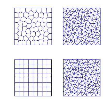
Figure 1: Test 7.1. Example of polygonal meshes: $\mathcal{V}_{1/8}$, $\mathcal{T}_{1/8}$, $\mathcal{Q}_{1/8}$, $\mathcal{W}_{1/8}$.

For the generation of the Voronoi meshes we used the code Polymesher [40]. The WEB-like meshes are composed by hexagons, generated starting from the triangular meshes $\{\mathcal{T}_{h}\}_{h}$ and randomly displacing the midpoint of each (non boundary) edge.
It is well known that the eigenvalues of the problem are given by

$$\lambda=\pi^{2}(n^{2}+m^{2})\qquad for\ n,m\in\mathbb{N},\ with\ n,m\neq 0.$$

We consider the VEM approximation problem (21) stemming from the stabilized bilinear form $\tilde{b}_{h}(\cdot,\cdot)$ where we use the stabilization (31) with the above mentioned selections of the stabilization parameters. We consider the polynomial degree of accuracy $k=1,2,3,4$ and we study the convergence of the errors $\epsilon_{h,\lambda}$ with respect to $h$ for the first six eigenvalues.

In Figures 2-5, we display the results for the sequence of Voronoi meshes $\mathcal{V}_{h}$, the sequence of meshes $\mathcal{T}_{h}$, $\mathcal{Q}_{h}$, and $\mathcal{W}_{h}$, respecitvely.

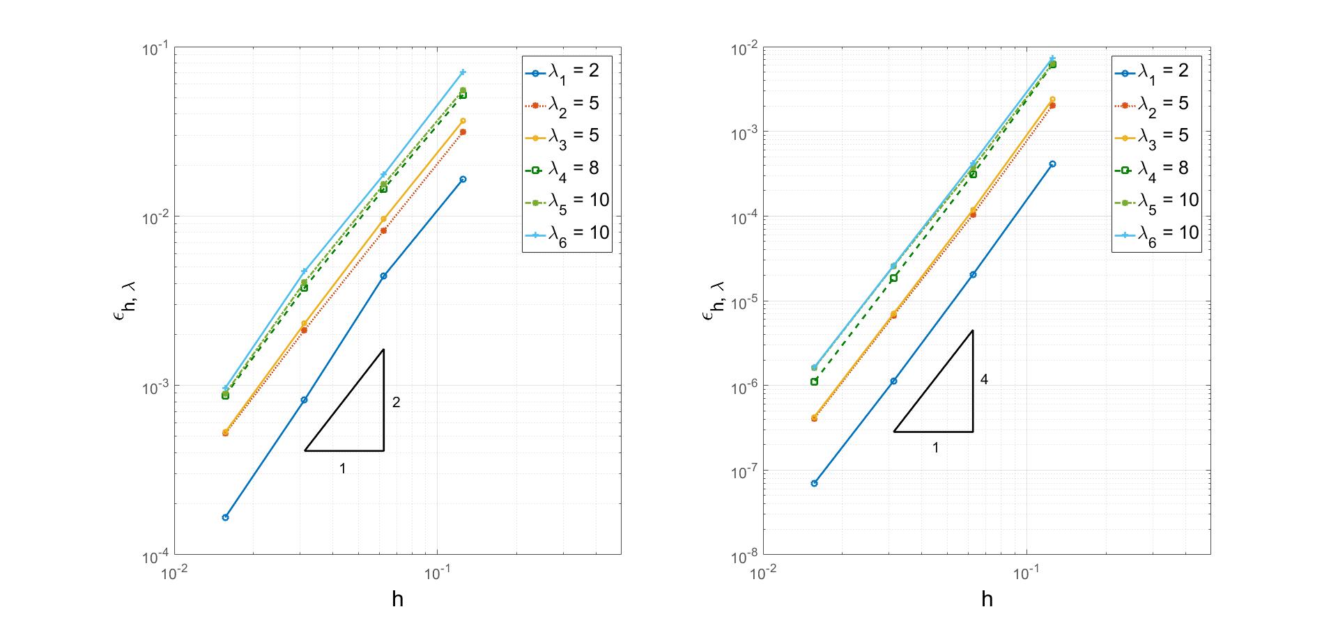
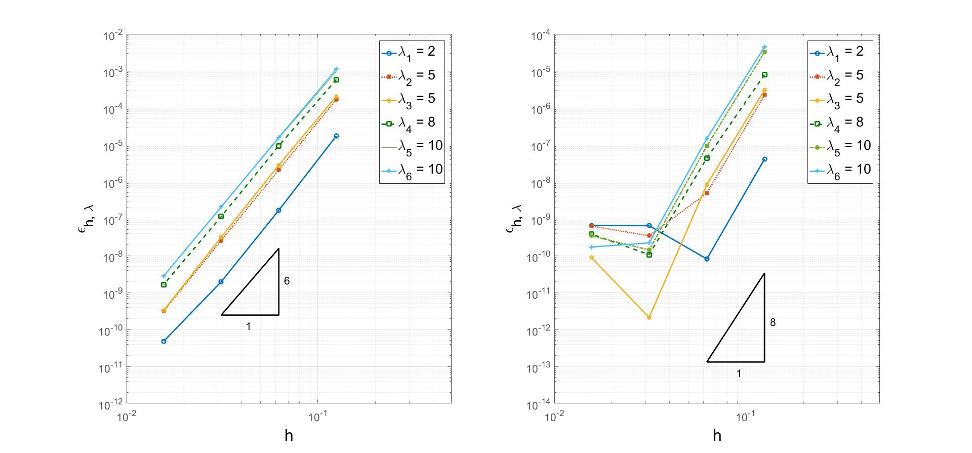
Figure 2: Test 7.1. Convergence plot for the eigenvalues for the sequence of meshes $\mathcal{V}_{h}$ with $k=1,2,3,4$.

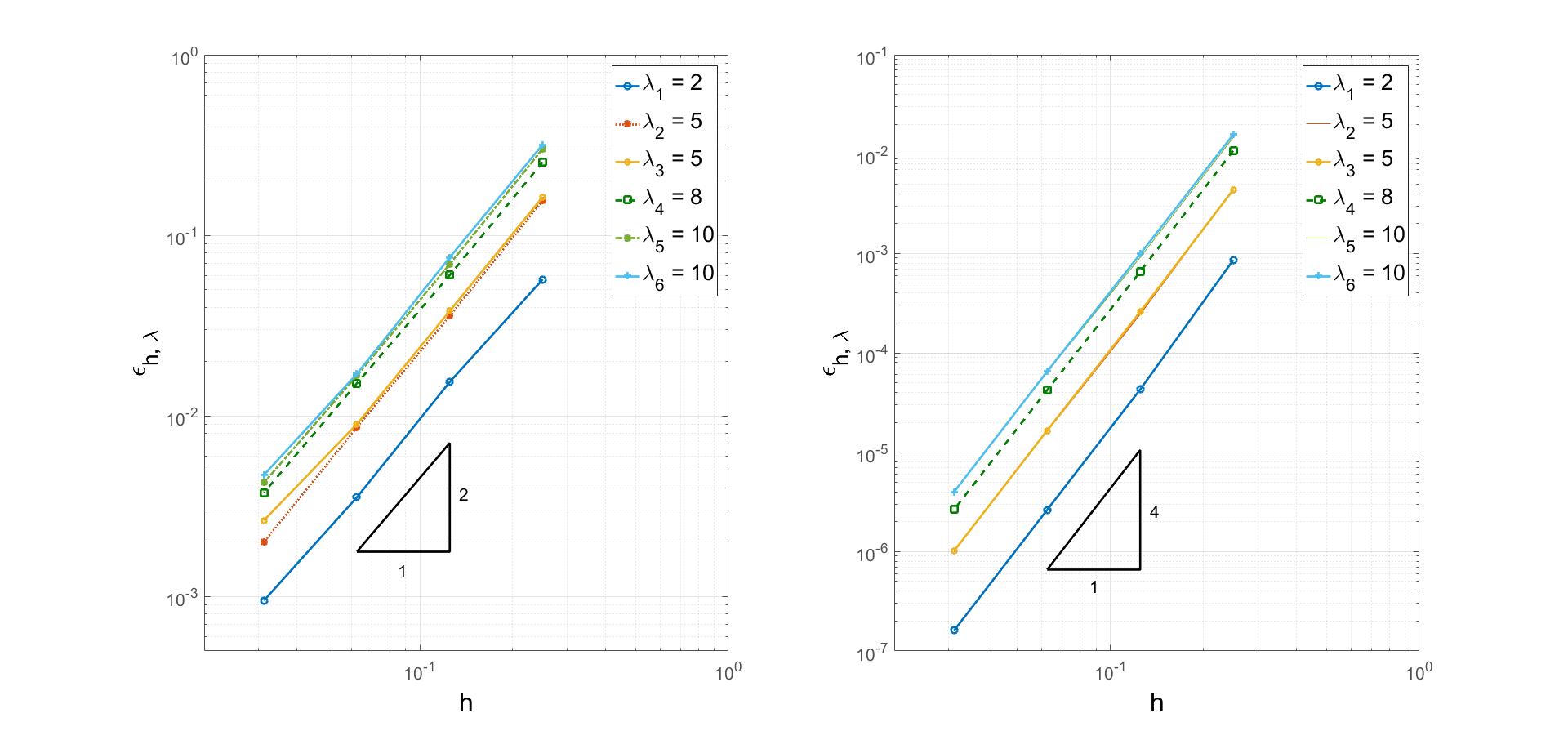
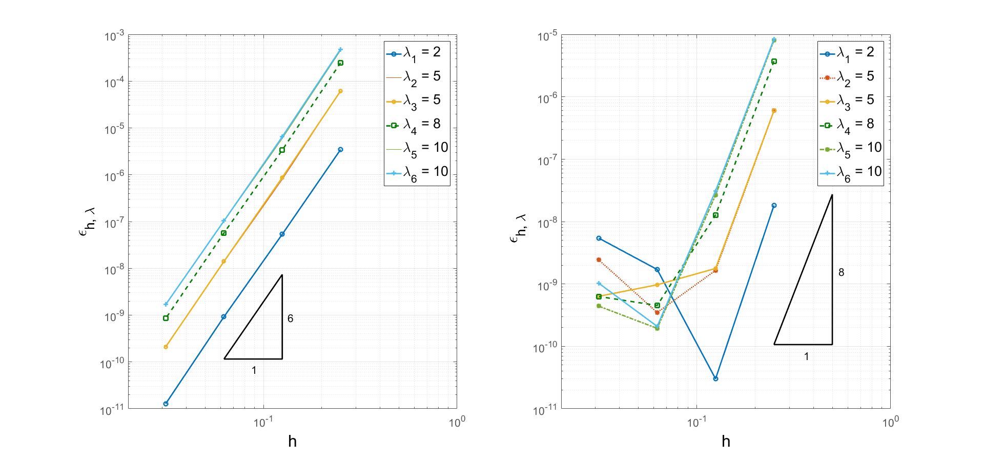
Figure 3: Test 7.1. Convergence plot for the eigenvalues for the sequence of meshes $\mathcal{T}_{h}$ with $k=1,2,3,4$.

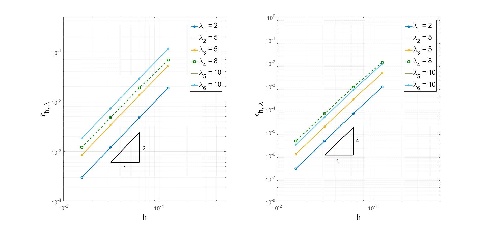
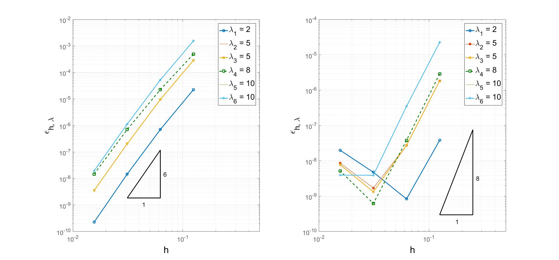
Figure 4: Test 7.1. Convergence plot for the eigenvalues for the sequence of meshes $\mathcal{Q}_{h}$ with $k=1,2,3,4$.

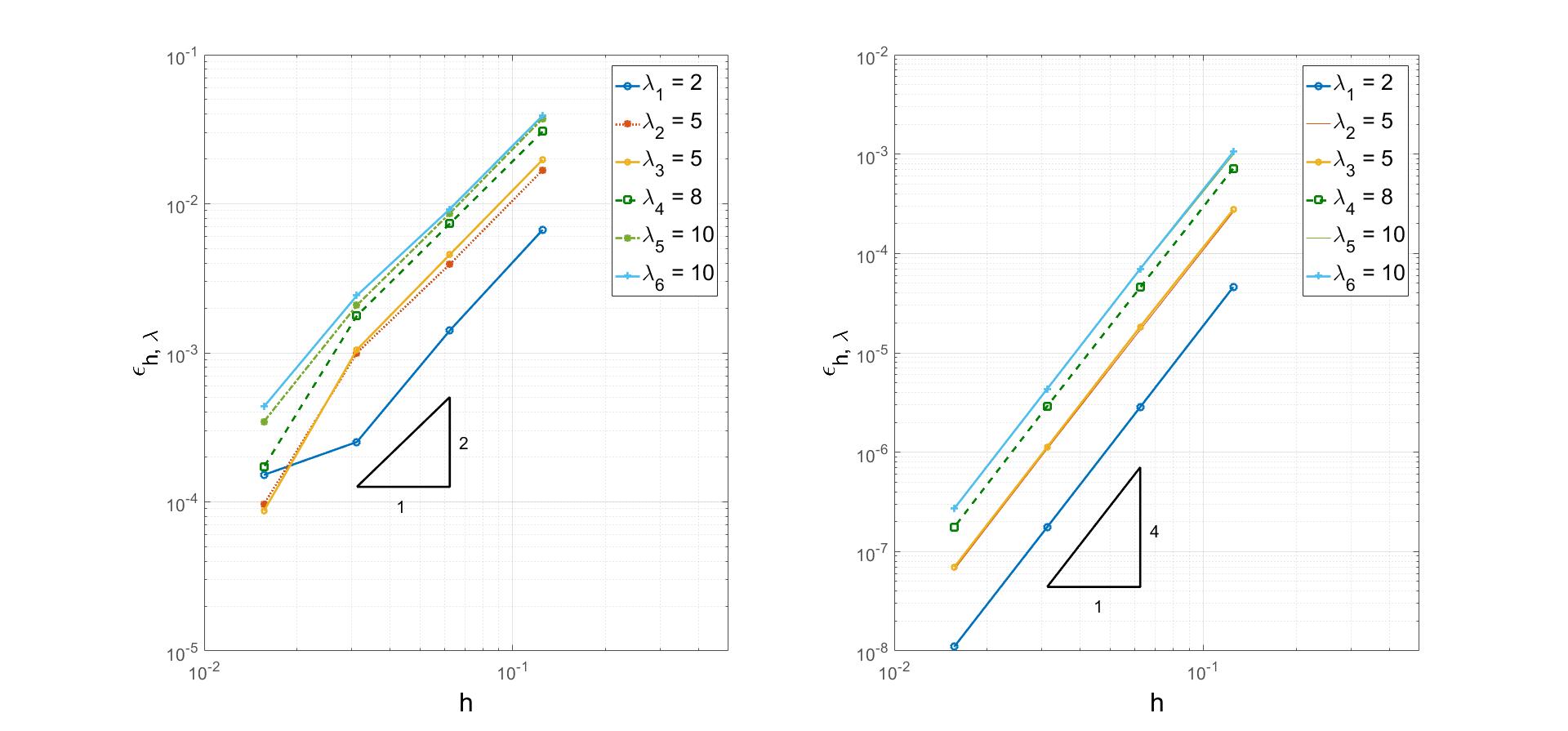
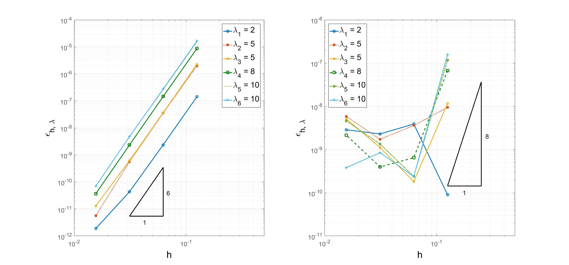
Figure 5: Test 7.1. Convergence plot for the eigenvalues for the sequence of meshes $\mathcal{W}_{h}$ with $k=1,2,3,4$.

We notice that for $k=1,2,3$ the theoretical predictions of Section 6.2 and Theorem 6.4 are confirmed for all the adopted meshes (noticed that the eigenfunctions are analytical). Whereas for $k=4$, the errors are close to the machine precision, but for small values of $h$ they become larger. This fact is natural and stems from the conditioning of the matrices involved in the computation of the VEM solution. Indeed, as in standard FEM, their condition numbers become larger when we consider higher VEM approximation degrees. The choice of the diagonal stabilization (32), cures this problem, see Figure 6: for small values of the mesh size $h$ we have errors close to the machine precision.

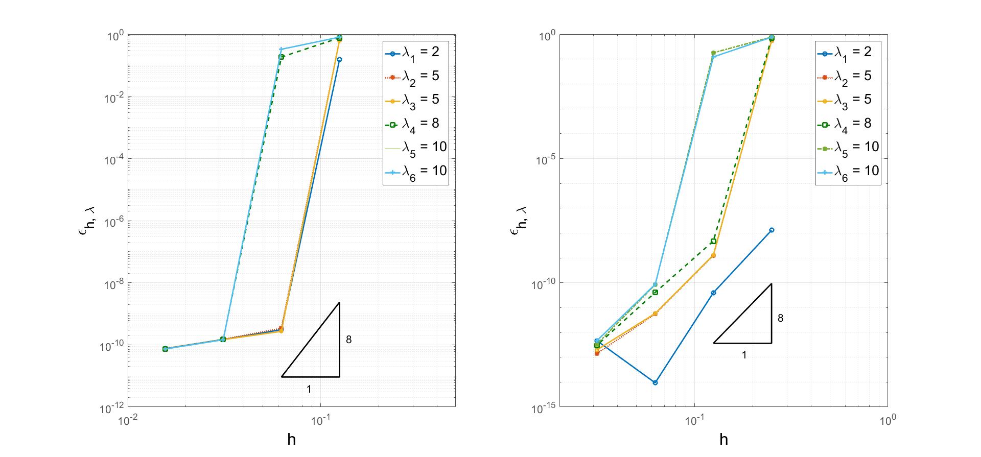
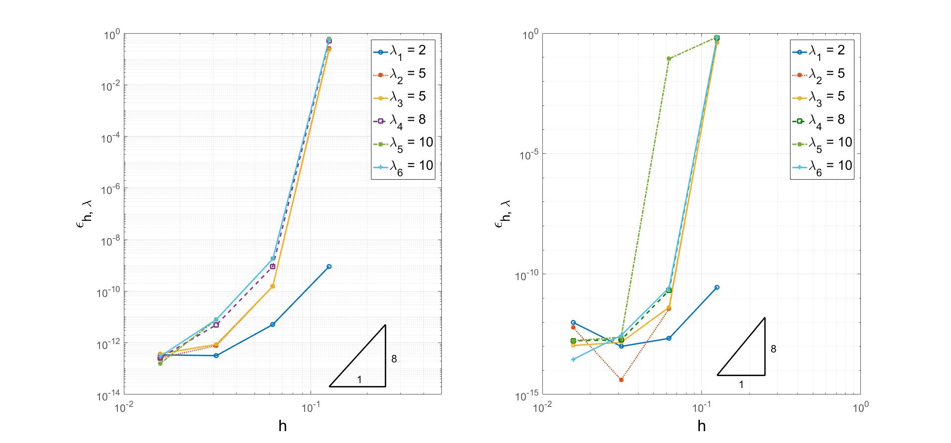
Figure 6: Test 7.1. Convergence plots for the eigenvalues for the sequence of meshes $\mathcal{V}_{h}$, $\mathcal{T}_{h}$, $\mathcal{Q}_{h}$, $\mathcal{W}_{h}$ with $k=4$ and diagonal stabilization (32).

Test 7.2.

We consider the same eigenvalue problem of Test 7.1 and we study the performance of the VEM discretization by comparing the non stabilized virtual method (18) with the stabilized one (21) with the stabilizations above introduced (cf. (31) and (32)). We use the polygonal decompositions listed above and polynomial degree of accuracy $k=1$ and $k=4$. In Table 1, 2, 3, 4 we show respectively the results for the sequences of meshes $\mathcal{V}_{h}$, $\mathcal{T}_{h}$, $\mathcal{Q}_{h}$ and $\mathcal{W}_{h}$ for the lowest degree $k=1$.

We notice that the matrices stemming from the non stabilized bilinear forms are not positive definite therefore we can not use the MATLAB routine eigs for sparse matrices. We overcome this problem by using for $k=1$ the MATLAB routine eig for full matrices. Whereas for $k=4$ we approximate the non stabilized bilinear forms by considering the stabilizations $\tilde{S}^{P}(\cdot,\cdot)$ in (31) with $\tau^{P}=1e-16$.

Moreover, we observe that the stabilized method (with both stabilizations) and the non stabilized method exhibit almost identical errors for the low order $k=1$, at least for this example and with the adopted meshes. For $k=4$, as observed above, the diagonal stabilization shows for small values of $h$ better performances.

	h	$\lambda_{1}=2\pi^{2}$	$\lambda_{2}=5\pi^{2}$	$\lambda_{4}=8\pi^{2}$	$\lambda_{5}=10\pi^{2}$
scalar	$1/8$	$1.65354e-2$	$3.65029e-2$	$5.19575e-2$	$7.10714e-2$
	$1/16$	$4.41849e-3$	$9.57783e-3$	$1.44610e-2$	$1.75766e-2$
	$1/32$	$8.20606e-4$	$2.32037e-3$	$3.76823e-3$	$4.71461e-3$
	$1/64$	$1.66238e-4$	$5.28919e-4$	$8.72219e-4$	$9.64257e-4$
diagonal	$1/8$	$1.24793e-2$	$1.31338e-2$	$2.71426e-1$	$3.95806e-1$
	$1/16$	$4.37700e-3$	$8.84813e-3$	$1.17396e-2$	$1.40754e-2$
	$1/32$	$8.64749e-4$	$2.39206e-3$	$3.79681e-3$	$4.74322e-3$
	$1/64$	$1.80022e-4$	$5.61628e-4$	$9.21153e-4$	$1.02400e-3$
non stab	$1/8$	$1.76616e-2$	$4.09826e-2$	$6.38367e-2$	$8.48765e-2$
	$1/16$	$4.61104e-3$	$1.02615e-2$	$1.55774e-2$	$1.92623e-2$
	$1/32$	$8.78350e-4$	$2.46463e-3$	$4.00339e-3$	$5.03841e-3$
	$1/64$	$1.80805e-4$	$5.66302e-4$	$9.34035e-4$	$1.04229e-3$

Table 1: Test 7.2. $\epsilon_{h,\lambda}$ for the sequence of meshes $\mathcal{V}_{h}$ with $k=1$ using stabilized form and non stabilized bilinear form (cf. (21) and (18)).

	h	$\lambda_{1}=2\pi^{2}$	$\lambda_{2}=5\pi^{2}$	$\lambda_{4}=8\pi^{2}$	$\lambda_{5}=10\pi^{2}$
scalar	$1/4$	$5.70169e-2$	$1.63047e-1$	$2.54353e-1$	$3.17892e-1$
	$1/8$	$1.54372e-2$	$3.81409e-2$	$6.02252e-2$	$7.55284e-2$
	$1/16$	$3.54381e-3$	$9.00524e-3$	$1.51584e-2$	$1.71163e-2$
	$1/32$	$9.51096e-4$	$2.64316e-3$	$3.76702e-3$	$4.71650e-3$
diagonal	$1/4$	$5.70169e-2$	$1.63047e-1$	$2.54353e-1$	$3.17892e-1$
	$1/8$	$1.54372e-2$	$3.81409e-2$	$6.02252e-2$	$7.55284e-2$
	$1/16$	$3.54381e-3$	$9.00524e-3$	$1.51584e-2$	$1.71163e-2$
	$1/32$	$9.51096e-4$	$2.64316e-3$	$3.76702e-3$	$4.71650e-3$
non stab	$1/4$	$5.70169e-2$	$1.63047e-1$	$2.54353e-1$	$3.17892e-1$
	$1/8$	$1.54372e-2$	$3.81409e-2$	$6.02252e-2$	$7.55284e-2$
	$1/16$	$3.54381e-3$	$9.00524e-3$	$1.51584e-2$	$1.71163e-2$
	$1/32$	$9.51096e-4$	$2.64316e-3$	$3.76702e-3$	$4.71650e-3$

Table 2: Test 7.2. $\epsilon_{h,\lambda}$ for the sequence of meshes $\mathcal{T}_{h}$ with $k=1$ using stabilized and non stabilized bilinear form (cf. (21) and (18)).

	h	$\lambda_{1}=2\pi^{2}$	$\lambda_{2}=5\pi^{2}$	$\lambda_{4}=8\pi^{2}$	$\lambda_{5}=10\pi^{2}$
scalar	$1/8$	$1.88180e-2$	$5.24872e-2$	$6.83463e-2$	$1.14922e-1$
	$1/16$	$4.79185e-3$	$1.34179e-2$	$1.88180e-2$	$2.92254e-2$
	$1/32$	$1.20310e-3$	$3.36892e-3$	$4.79185e-3$	$7.30994e-3$
	$1/64$	$3.01091e-4$	$8.43074e-4$	$1.20310e-3$	$1.82733e-3$
diagonal	$1/8$	$1.34980e-2$	$3.00644e-2$	$1.31356e-1$	$2.29494e-1$
	$1/16$	$4.46838e-3$	$1.21017e-2$	$1.34980e-2$	$2.61752e-2$
	$1/32$	$1.18304e-3$	$3.28834e-3$	$4.46838e-3$	$7.12721e-3$
	$1/64$	$2.99840e-4$	$8.38065e-4$	$1.18304e-3$	$1.81604e-3$
non stab	$1/8$	$1.96813e-2$	$5.61954e-2$	$8.40240e-2$	$1.24337e-1$
	$1/16$	$4.84403e-3$	$1.36304e-2$	$1.96812e-2$	$2.97190e-2$
	$1/32$	$1.20633e-3$	$3.38191e-3$	$4.84400e-3$	$7.33940e-3$
	$1/64$	$3.01292e-4$	$8.43879e-4$	$1.20632e-3$	$1.82915e-3$

Table 3: Test 7.2. $\epsilon_{h,\lambda}$ for the sequence of meshes $\mathcal{Q}_{h}$ with $k=1$ using stabilized and non stabilized bilinear form (cf. (21) and (18)).

	h	$\lambda_{1}=2\pi^{2}$	$\lambda_{2}=5\pi^{2}$	$\lambda_{4}=8\pi^{2}$	$\lambda_{5}=10\pi^{2}$
scalar	$1/8$	$6.69124e-3$	$1.97714e-2$	$3.05479e-2$	$3.91016e-2$
	$1/16$	$1.41184e-3$	$4.55875e-3$	$7.34674e-3$	$9.20778e-3$
	$1/32$	$2.52359e-4$	$1.04890e-3$	$1.77164e-3$	$2.42393e-3$
	$1/64$	$1.51786e-4$	$8.71580e-5$	$1.71693e-4$	$4.35676e-4$
diagonal	$1/8$	$5.41188e-3$	$1.40607e-2$	$1.70178e-2$	$1.73017e-2$
	$1/16$	$1.19325e-3$	$3.91139e-3$	$6.05178e-3$	$7.56699e-3$
	$1/32$	$2.07297e-4$	$9.27293e-4$	$1.56408e-3$	$2.16149e-3$
	$1/64$	$1.62207e-4$	$6.16087e-5$	$1.28674e-4$	$3.81062e-4$
non stab	$1/8$	$6.06830e-3$	$1.83072e-2$	$2.85770e-2$	$3.71010e-2$
	$1/16$	$1.23021e-3$	$4.12929e-3$	$6.68713e-3$	$8.43576e-3$
	$1/32$	$2.09025e-4$	$9.37654e-3$	$1.59110e-3$	$2.20261e-3$
	$1/64$	$1.62237e-4$	$6.14193e-5$	$1.28187e-4$	$3.80246e-4$

Table 4: Test 7.2. $\epsilon_{h,\lambda}$ for the sequence of meshes $\mathcal{W}_{h}$ with $k=1$ using stabilized and non stabilized bilinear form (cf. (21) and (18)).

	h	$\lambda_{1}=2\pi^{2}$	$\lambda_{2}=5\pi^{2}$	$\lambda_{4}=8\pi^{2}$	$\lambda_{5}=10\pi^{2}$
scalar	$1/8$	$4.08694e-08$	$3.03255e-06$	$7.85639e-06$	$4.42827e-05$
	$1/16$	$8.10132e-11$	$8.32945e-09$	$4.36448e-08$	$1.47462e-07$
	$1/32$	$6.45147e-10$	$2.10939e-12$	$1.06202e-10$	$2.21067e-10$
	$1/64$	$6.54068e-10$	$8.81773e-11$	$3.81458e-10$	$1.70565e-10$
diagonal	$1/8$	$1.50768e-01$	$6.34515e-01$	$7.65639e-01$	$8.05257e-01$
	$1/16$	$3.09080e-10$	$2.72011e-10$	$1.83621e-01$	$3.27562e-01$
	$1/32$	$1.48304e-10$	$1.47156e-10$	$1.50437e-10$	$1.45682e-10$
	$1/64$	$7.55412e-11$	$7.34704e-11$	$7.29845e-11$	$7.36543e-11$
non stab	$1/8$	$4.09387e-08$	$3.04614e-06$	$7.91452e-06$	$4.46984e-05$
	$1/16$	$8.09754e-11$	$8.34021e-09$	$4.37285e-08$	$1.47462e-07$
	$1/32$	$6.44920e-10$	$1.28349e-12$	$1.05962e-10$	$2.22278e-10$
	$1/64$	$6.54187e-10$	$8.82860e-11$	$3.81741e-10$	$1.70739e-10$

Table 5: Test 7.2. $\epsilon_{h,\lambda}$ for the sequence of meshes $\mathcal{V}_{h}$ with $k=4$ using stabilized and non stabilized bilinear form (cf. (21) and (18)).

	h	$\lambda_{1}=2\pi^{2}$	$\lambda_{2}=5\pi^{2}$	$\lambda_{4}=8\pi^{2}$	$\lambda_{5}=10\pi^{2}$
scalar	$1/4$	$1.81535e-08$	$5.97563e-07$	$3.71995e-06$	$8.31271e-06$
	$1/8$	$3.01783e-11$	$1.77195e-09$	$1.27304e-08$	$3.09954e-08$
	$1/16$	$1.70546e-09$	$9.69266e-10$	$4.52175e-10$	$2.09013e-10$
	$1/32$	$5.42087e-09$	$6.33818e-10$	$6.29748e-10$	$1.02642e-09$
diagonal	$1/4$	$1.29083e-08$	$5.43812e-01$	$7.14882e-01$	$7.59974e-01$
	$1/8$	$3.97711e-11$	$1.30016e-09$	$4.74659e-09$	$1.22090e-01$
	$1/16$	$9.35909e-15$	$5.81516e-12$	$4.05619e-11$	$8.57591e-11$
	$1/32$	$4.62015e-13$	$1.97548e-13$	$3.04890e-13$	$4.64787e-13$
non stab	$1/4$	$1.81674e-08$	$5.97558e-07$	$3.71998e-06$	$8.31282e-06$
	$1/8$	$3.16576e-11$	$1.77308e-09$	$1.27284e-08$	$3.09934e-08$
	$1/16$	$1.70289e-09$	$9.67242e-10$	$4.51765e-10$	$2.07578e-10$
	$1/32$	$5.41948e-09$	$6.33574e-10$	$6.30034e-10$	$1.02564e-09$

Table 6: Test 7.2. $\epsilon_{h,\lambda}$ for the sequence of meshes $\mathcal{T}_{h}$ with $k=4$ using stabilized and non stabilized bilinear form (cf. (21) and (18)).

	h	$\lambda_{1}=2\pi^{2}$	$\lambda_{2}=5\pi^{2}$	$\lambda_{4}=8\pi^{2}$	$\lambda_{5}=10\pi^{2}$
scalar	$1/8$	$3.81184e-08$	$1.84365e-06$	$2.90250e-06$	$2.25968e-05$
	$1/16$	$8.34788e-10$	$2.72448e-08$	$3.80267e-08$	$3.49035e-07$
	$1/32$	$4.75842e-09$	$1.33322e-09$	$6.22220e-10$	$3.91731e-09$
	$1/64$	$1.99260e-08$	$7.75128e-09$	$5.20401e-09$	$3.93187e-09$
diagonal	$1/8$	$9.12570e-10$	$2.24086e-01$	$5.15054e-01$	$5.83981e-01$
	$1/16$	$5.13094e-12$	$1.54985e-10$	$9.12586e-10$	$1.80273e-09$
	$1/32$	$3.20728e-13$	$8.71979e-13$	$5.02799e-12$	$8.12758e-12$
	$1/64$	$3.42866e-13$	$3.75371e-13$	$2.60074e-13$	$2.95603e-13$
non stab	$1/8$	$3.81202e-08$	$1.84390e-06$	$2.90262e-06$	$2.26029e-05$
	$1/16$	$8.34530e-10$	$2.72483e-08$	$3.80285e-08$	$3.49125e-07$
	$1/32$	$4.75887e-09$	$1.33338e-09$	$6.22323e-10$	$3.91791e-09$
	$1/64$	$1.99268e-08$	$7.75217e-09$	$5.20491e-09$	$3.93284e-09$

Table 7: Test 7.2. $\epsilon_{h,\lambda}$ for the sequence of meshes $\mathcal{Q}_{h}$ with $k=4$ using stabilized and non stabilized bilinear form (cf. (21) and (18)).

	h	$\lambda_{1}=2\pi^{2}$	$\lambda_{2}=5\pi^{2}$	$\lambda_{4}=8\pi^{2}$	$\lambda_{5}=10\pi^{2}$
scalar	$1/8$	$8.97772e-11$	$1.15946e-08$	$6.67721e-08$	$1.55547e-07$
	$1/16$	$3.88976e-09$	$1.81961e-10$	$6.45283e-10$	$2.37503e-10$
	$1/32$	$2.29197e-09$	$1.10633e-09$	$3.96093e-10$	$8.44730e-10$
	$1/64$	$2.86708e-09$	$5.13913e-09$	$2.15705e-09$	$3.80039e-10$
diagonal	$1/8$	$2.85391e-11$	$4.01092e-01$	$6.25071e-01$	$6.71266e-01$
	$1/16$	$2.13639e-13$	$4.20180e-12$	$2.11403e-11$	$2.73006e-11$
	$1/32$	$9.95303e-14$	$1.45713e-13$	$1.83942e-13$	$2.82788e-13$
	$1/64$	$9.81984e-13$	$1.08277e-13$	$1.69903e-13$	$2.86532e-14$
non stab	$1/8$	$9.63542e-11$	$1.16189e-08$	$6.70782e-08$	$1.56541e-07$
	$1/16$	$3.85156e-09$	$2.89697e-10$	$5.72624e-10$	$2.81162e-10$
	$1/32$	$2.31192e-09$	$1.08736e-09$	$3.66330e-10$	$8.35562e-10$
	$1/64$	$2.86720e-09$	$5.13207e-09$	$2.14902e-09$	$3.75120e-10$

Table 8: Test 7.2. $\epsilon_{h,\lambda}$ for the sequence of meshes $\mathcal{W}_{h}$ with $k=4$ using stabilized and non stabilized bilinear form (cf. (21) and (18)).

We can observe that the results in the tables confirm the theoretical rates of convergence stated in Section 6.1 and 6.2. In Table 2 we observe that the errors, as expected, are identical for the three cases. Indeed for the triangular meshes $\mathcal{T}_{h}$ the virtual space $V_{h}^{1}(T)$ corresponds to the space of linear polynomials, then

$$S^{T}\Big{(}(I-\Pi_{1}^{\nabla})u_{h},(I-\Pi_{1}^{\nabla})v_{h}\Big{)}=\tilde{S}^{T}\Big{(}(I-\Pi_{1}^{0})u_{h},(I-\Pi_{1}^{0})v_{h}\Big{)}=0$$

for all $u_{h},v_{h}\in V_{h}^{1}(T)$, therefore the non stabilized method (18) and the stabilized method (21) are equivalent.

Finally, we test the robustness of the method with respect to the stabilization parameter $\tau_{P}$ in (31). In Figure 7 we plot the first four eigenvalues obtained by using the method (21) with $k=1$ for the sequence of Voronoi meshes $\mathcal{V}_{h}$ in Test 7.1 as a function of stabilization parameter $\tau_{P}$.

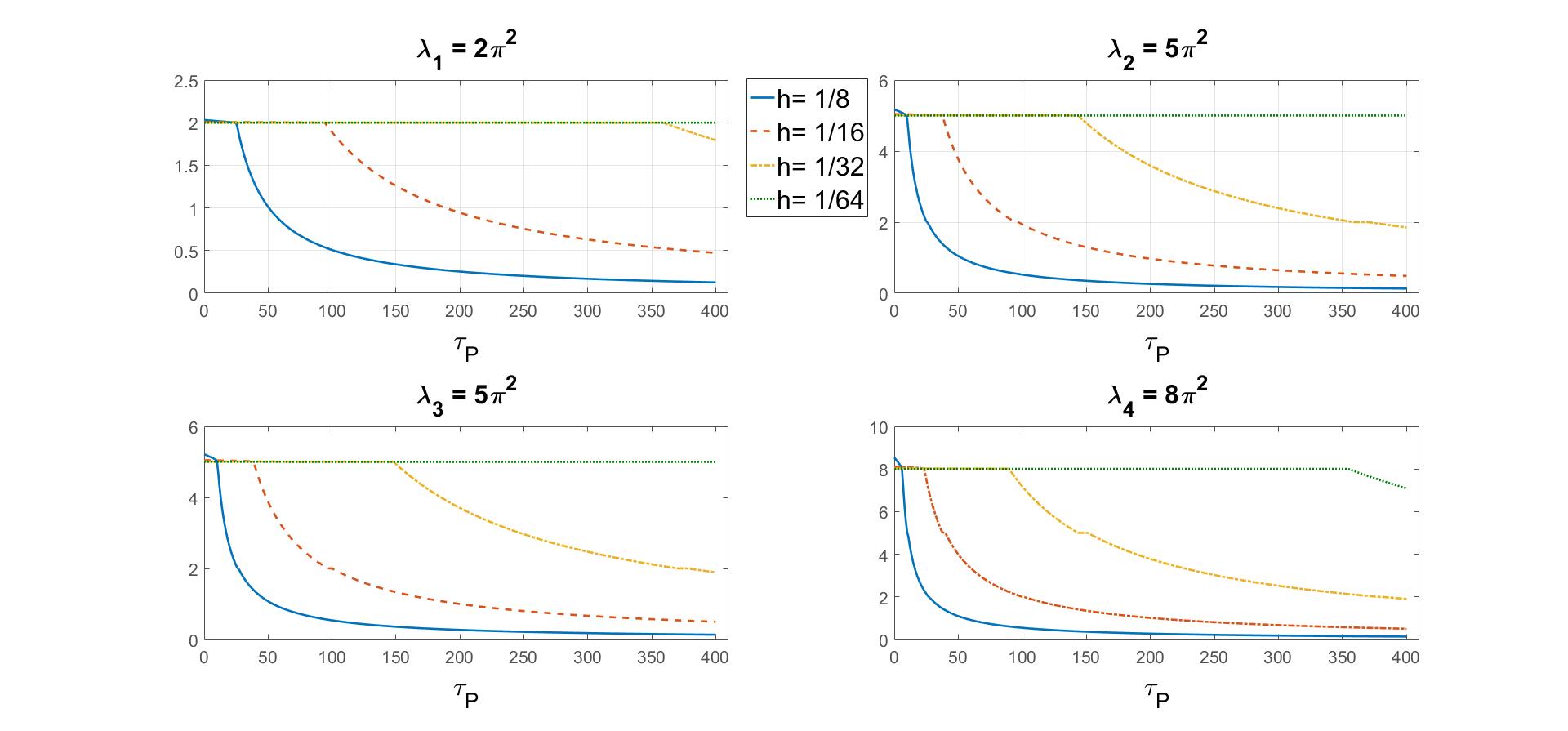
Figure 7: Test 7.2. First four eigenvalues as a function of the stabilization parameter $\tau_{P}$ (on the abscissas axis).

We observe that the method is robust with respect to the stabilization parameter $\tau_{P}$. For reasonable values of $\tau_{P}$ and for small enough values of the mesh size $h$, the numerical eigenvalues are not effected by the selection of the stabilization parameter. Moreover, as expected, the “critical parameter”, i.e. the minimum value $\tau_{P}$ for which the associated method fails, goes like $h^{-2}$.

Test 7.3.

This test problem, as the following one, is taken from the benchmark singular solution set in [31]. We consider the square domain $\Omega=(-1,1)^{2}$ splitted into two subdomains $\Omega_{\delta}$ and $\Omega_{1}$ (see the left plot in Figure 8), and we study the eigenvalue problem on the square with Neumann homogeneous boundary conditions and discontinuous diffusivity.

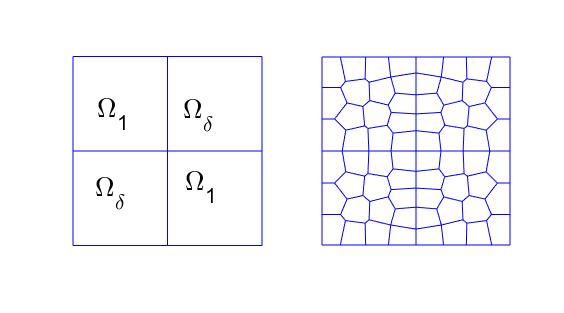
Figure 8: Test 7.3. Left plot: subdivision of $\Omega$ into the subdomains $\Omega_{\delta}$ and $\Omega_{1}$. Right plot: Example of locally Voronoi decomposition of $\Omega$.

In this test we consider the continuous bilinear form

$$a_{\mathbb{K}}^{P}(u,v):=\int_{P}\mathbb{K}\nabla u\cdot\nabla v\,{\rm d}\bf{x}$$

whose virtual approximation (see [14]) is given by

$$a_{h,\mathbb{K}}^{P}(u_{h},v_{h})=\int_{P}\mathbb{K}\Pi_{k-1}^{0}\nabla u_{h}\cdot\Pi_{k-1}^{0}\nabla v_{h}\,{\rm d}{\bf{x}}+S^{P}\Big{(}(I-\Pi_{k}^{\nabla})u_{h},(I-\Pi_{k}^{\nabla})v_{h}\Big{)}$$ (33)

to be used in place of $a_{h}^{P}(u_{h},v_{h})$ (cf. (13)) in Problem (22). We take $\mathbb{K}_{|\Omega_{1}}=I$ and $\mathbb{K}_{|\Omega_{\delta}}=\delta I$ with four different values of $\delta$, namely $\delta=0.50,0.10,0.01,1e-8$.

We apply the Virtual Element method (21) with the scalar stabilization (31) using a sequence of Voronoi meshes with mesh diameter $h=1/2,1/4,1/8,1/16$ (see the right plot in Figure 8 for an example of the adopted meshes). We show the plot of the convergence for the first and second computed eigenvalues in Figures 9 and 10. We compute the errors $\epsilon_{h,\lambda}$ by comparing our results with the values given in [31].

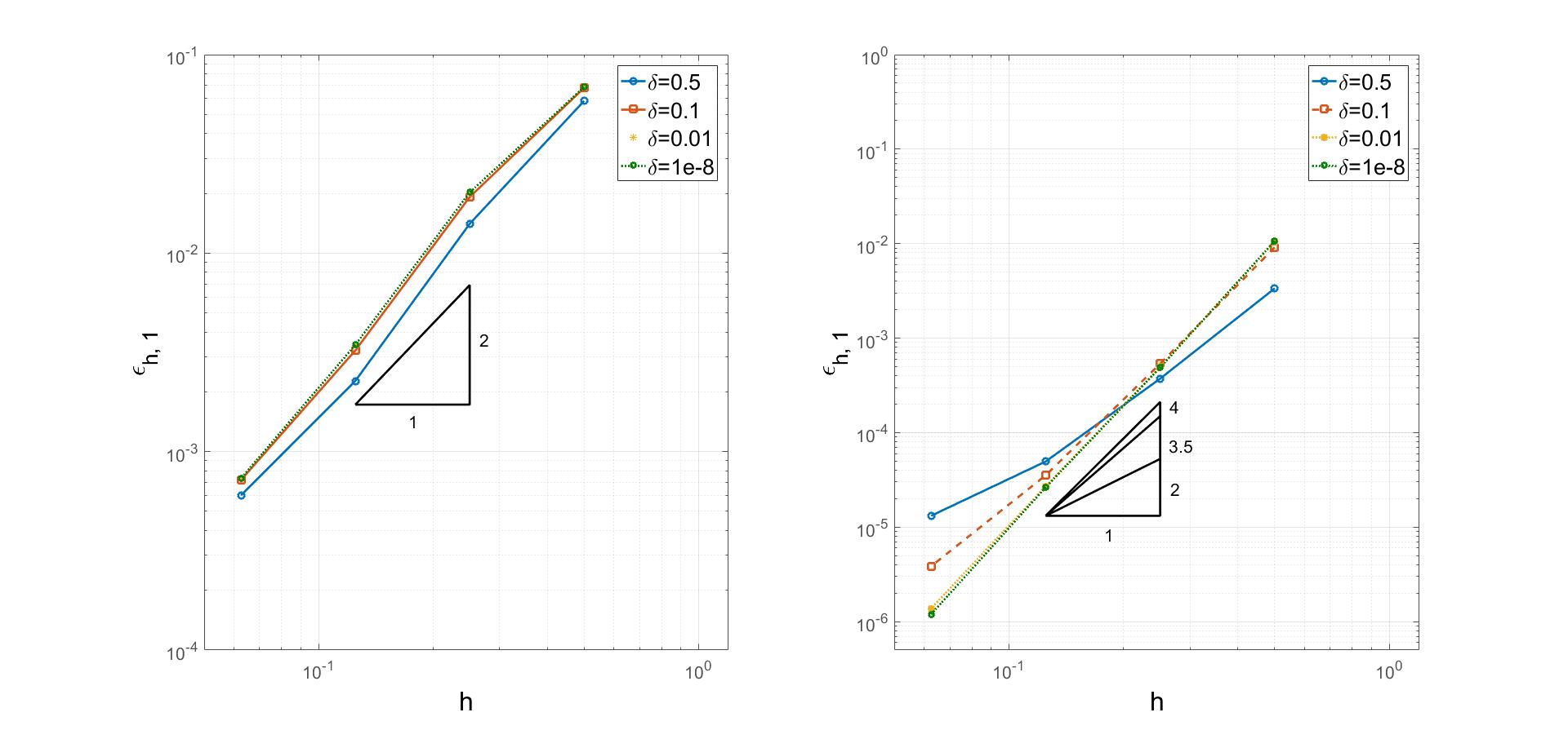
Figure 9: Test 7.3. Convergence plots for the first eigenvalue and different values of the diffusivity. Left plot: $k=1$. Right plot: $k=2$.

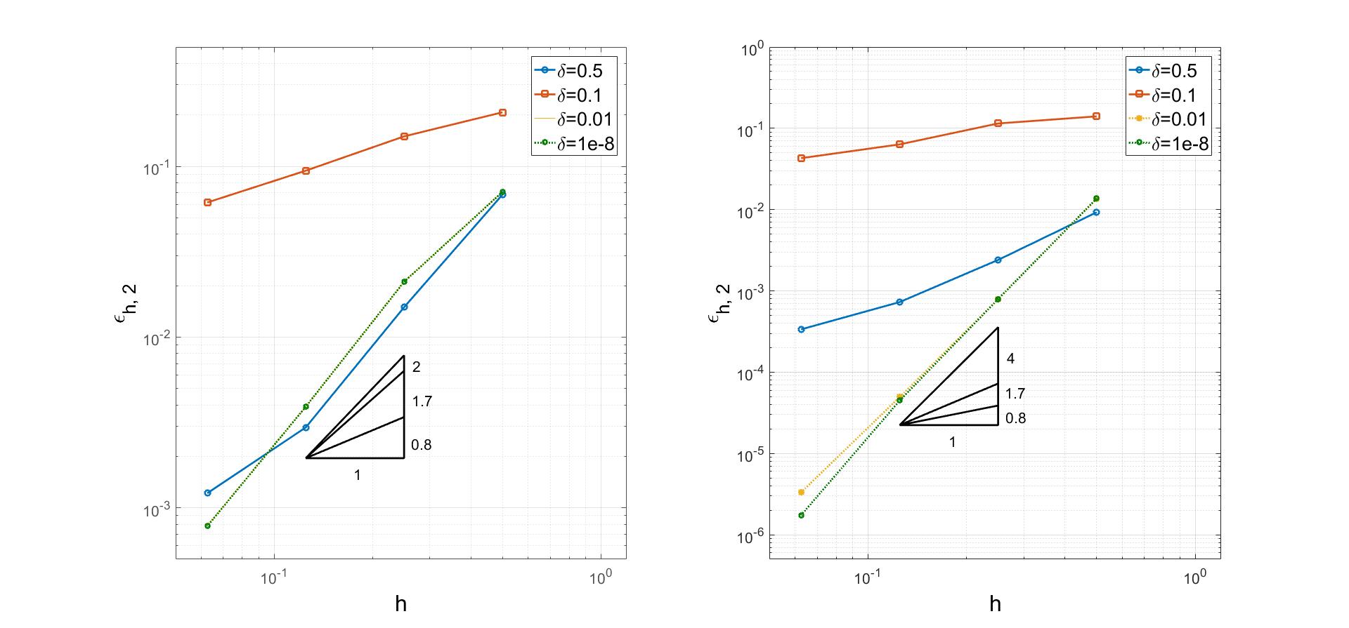
Figure 10: Test 7.3. Convergence plots for the second eigenvalue and different values of the diffusivity. Left plot: $k=1$. Right plot: $k=2$.

We can observe, in accordance with Theorem 6.4, different rates of convergence that are determined by the polynomail order of the method and by the regularity of the corresponding exact eigenfunctions [31]. Taking this into account, the method is overall optimal, and thus stable with respect to discontinuities in the diffusivity tensor.

Test 7.4.

In the last test we solve the eigenvalue problem with Neumann boundary conditions on the non-convex L-shaped domain $\Omega=\Omega_{big}\setminus\Omega_{small}$, where $\Omega_{big}$ is the square $(-1,1)^{2}$ and $\Omega_{small}$ is the square $(0,1)\times(-1,0)$. Also this test problem is taken from the benchmark singular solution set [31]. We apply the Virtual Element method (21) with the scalar stabilization (31). We use the sequence of Voronoi decomposition of the domain $\Omega$ in Figure 11. The convergence results relative to the first and the third eigenvalues are shown in Figure 12. For the first eigenvalue we observe a lower rate of convergence due to the fact that the corresponding eigenfunction is in $H^{1+r}$, with $r=2/3-\varepsilon$ for any $\varepsilon>0$ (see [31]), while the third eigenfunction is analytical therefore we obtain the optimal order of convergence. The error slopes validate the predicted convergence rates stated in Section 6.2, and confirm the optimality of the method also on non-convex domains.

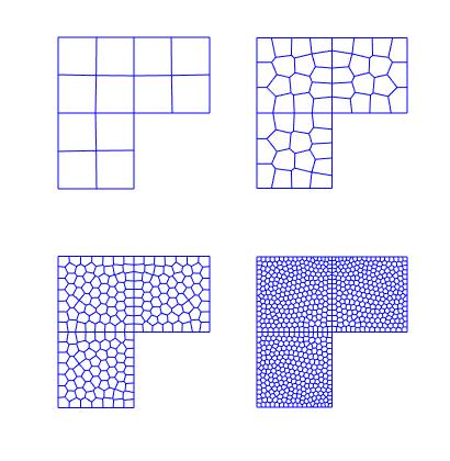
Figure 11: Test 7.4. Adopted family of meshes for the L-shaped domain $\Omega$.

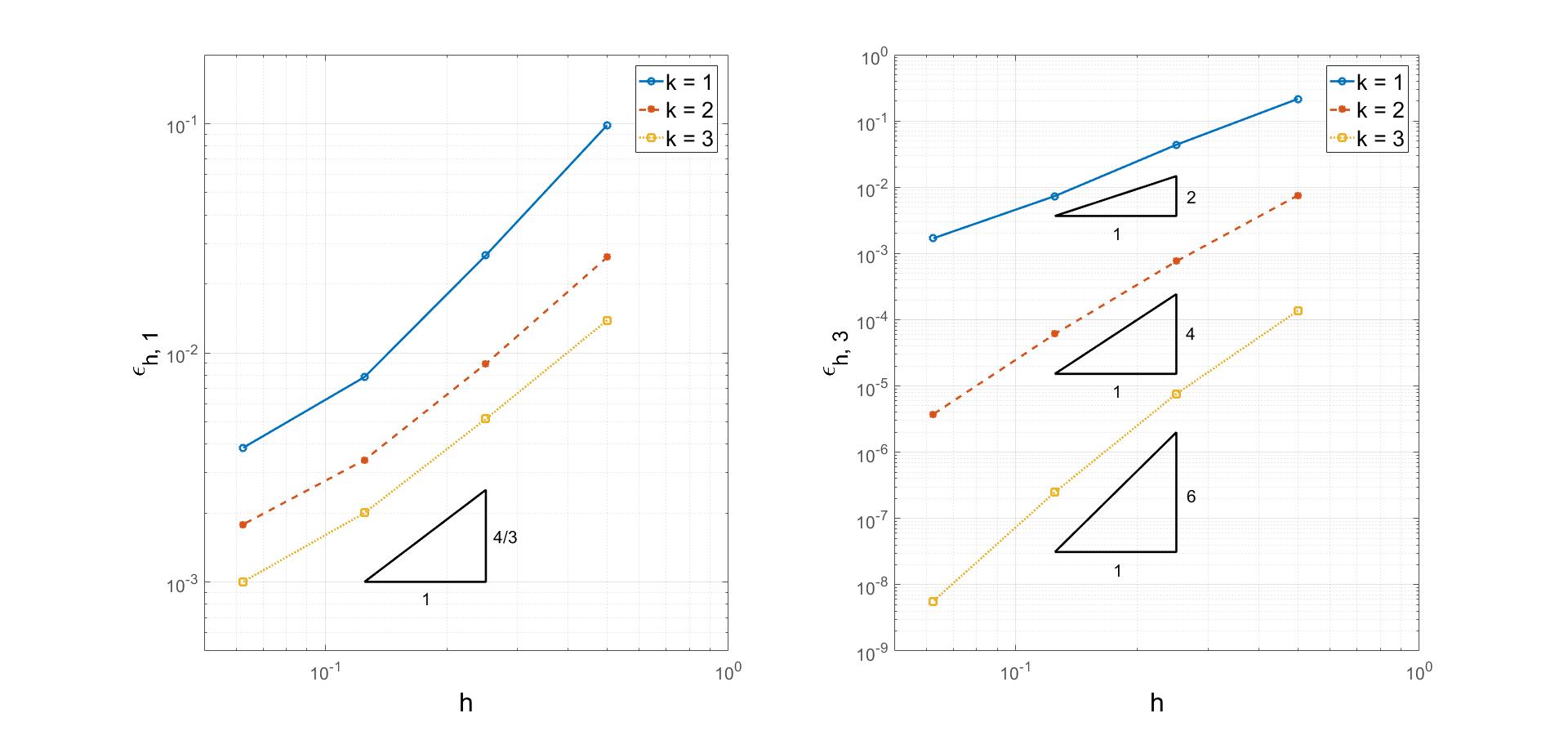
Figure 12: Test 7.4. Convergence plot for the eigenvalues for the L-shaped domain for the sequence of meshes in Figure 11 and $k=1,2,3$. Left plot: first eigenvalue. Right plot: third eigenvalue.

8 Conclusions

We have analyzed the VEM approximation of elliptic eigenvalue problems. We proved the method is of optimal order both in the approximation of the eigenfunctions and of the eigenvalues. A wide set of numerical test confirm the theoretical results. Further development consists in studying the VEM approximation of eigenvalue problems in mixed form, a posteriori error estimates and convergence of adaptive VEM for eigenvalue problems.

References

- [1] S. Agmon. Lectures on elliptic boundary value problems. Prepared for publication by B. Frank Jones, Jr. with the assistance of George W. Batten, Jr. Van Nostrand Mathematical Studies, No. 2. D. Van Nostrand Co., Inc., Princeton, N.J.-Toronto-London, 1965.
- [2] B. Ahmad, A. Alsaedi, F. Brezzi, L. D. Marini, and A. Russo. Equivalent projectors for virtual element methods. Comput. Math. Appl., 66(3):376–391, 2013.
- [3] P. F. Antonietti, L. Beirão da Veiga, D. Mora, and M. Verani. A stream virtual element formulation of the Stokes problem on polygonal meshes. SIAM J. Numer. Anal., 52(1):386–404, 2014.
- [4] P. F. Antonietti, L. Beirão Da Veiga, S. Scacchi, and M. Verani. A Virtual Element method for the Cahn-Hilliard equation with polygonal meshes. SIAM J. Numer. Anal., 54(1):34–56, 2016.
- [5] B. Ayuso de Dios, K. Lipnikov, and G. Manzini. The nonconforming virtual element method. ESAIM Math. Model. Numer. Anal., 50(3), 2016.
- [6] I. Babuška and J. Osborn. Eigenvalue problems. In Handbook of numerical analysis, Vol. II, Handb. Numer. Anal., II, pages 641–787. North-Holland, Amsterdam, 1991.
- [7] L. Beirão da Veiga, F. Brezzi, L. D. Marini, and A. Russo. and -conforming virtual element methods. Numer. Math., 133(2):303–332, 2016.
- [8] L. Beirão da Veiga, F. Brezzi, A. Cangiani, G. Manzini, L. D. Marini, and A. Russo. Basic principles of virtual element methods. Math. Models Methods Appl. Sci., 23(1):199–214, 2013.
- [9] L. Beirão da Veiga, F. Brezzi, and L. D. Marini. Virtual elements for linear elasticity problems. SIAM J. Numer. Anal., 51(2):794–812, 2013.
- [10] L. Beirão da Veiga, F. Brezzi, L. D. Marini, and A. Russo. The hitchhiker’s guide to the virtual element method. Math. Models Methods Appl. Sci., 24(8):1541–1573, 2014.
- [11] L. Beirão Da Veiga, F. Brezzi, L. D. Marini, and A. Russo. Mixed Virtual Element Methods for general second order elliptic problems on polygonal meshes. ESAIM Math. Model. Numer. Anal., 50(3):727–747, 2016.
- [12] L. Beirão Da Veiga, F. Brezzi, L. D. Marini, and A. Russo. Serendipity Face and Edge VEM spaces. RendLincei, 28(1):143?–180, 2016.
- [13] L. Beirão Da Veiga, F. Brezzi, L. D. Marini, and A. Russo. Serendipity Nodal VEM spaces. Comput. & Fluids, 141:2–12, 2016.
- [14] L. Beirão da Veiga, F. Brezzi, L. D. Marini, and A. Russo. Virtual Element Method for general second-order elliptic problems on polygonal meshes. Math. Models Methods Appl. Sci., 26(4):729–750, 2016.
- [15] L. Beirão da Veiga, A. Chernov, L. Mascotto, and A. Russo. Basic principles of virtual elements on quasiuniform meshes. Math. Models Methods Appl. Sci., 26(8):1567–1598, 2016.
- [16] L. Beirão Da Veiga, F. Dassi, and A. Russo. High-order Virtual Element Method on polyhedral meshes. arXiv preprint arXiv:1703.02882, 2017.
- [17] L. Beirão da Veiga, C. Lovadina, and D. Mora. A Virtual Element Method for elastic and inelastic problems on polytope meshes. Comput. Methods Appl. Mech. Engrg., 295:327–346, 2015.
- [18] L. Beirão Da Veiga, C. Lovadina, and G. Vacca. Divergence free virtual elements for the Stokes problem on polygonal meshes. ESAIM Math. Model. Numer. Anal., 51(2):509–535, 2017.
- [19] L. Beirão da Veiga and G. Manzini. A virtual element method with arbitrary regularity. IMA J. Numer. Anal., 34(2):759–781, 2014.
- [20] L. Beirão da Veiga and G. Manzini. Residual a posteriori error estimation for the virtual element method for elliptic problems. ESAIM Math. Model. Numer. Anal., 49(2):577–599, 2015.
- [21] M. F. Benedetto, S. Berrone, A. Borio, S. Pieraccini, and S. Scialò. A hybrid mortar virtual element method for discrete fracture network simulations. J. Comput. Phys., 306:148–166, 2016.
- [22] M. F. Benedetto, S. Berrone, S. Pieraccini, and S. Scialò. The virtual element method for discrete fracture network simulations. Comput. Methods Appl. Mech. Engrg., 280:135–156, 2014.
- [23] D. Boffi. Finite element approximation of eigenvalue problems. Acta Numer., 19:1–120, 2010.
- [24] D. Boffi, F. Brezzi, and L. Gastaldi. On the problem of spurious eigenvalues in the approximation of linear elliptic problems in mixed form. Math. Comp., 69(229):121–140, 2000.
- [25] S. C. Brenner and L. R. Scott. The mathematical theory of finite element methods, volume 15 of Texts in Applied Mathematics. Springer, New York, third edition, 2008.
- [26] F. Brezzi, Richard S. Falk, and L. D. Marini. Basic principles of mixed virtual element methods. ESAIM Math. Model. Numer. Anal., 48(4):1227–1240, 2014.
- [27] F. Brezzi and L. D. Marini. Virtual element methods for plate bending problems. Comput. Methods Appl. Mech. Engrg., 253:455–462, 2013.
- [28] A. Cangiani, E. H. Georgoulis, T. Pryer, and O. J. Sutton. A posteriori error estimates for the virtual element method. arXiv preprint arXiv:1603.05855, 2016.
- [29] A. Cangiani, G. Manzini, and O. J. Sutton. Conforming and nonconforming virtual element methods for elliptic problems. arXiv preprint arXiv:1507.03543, 2015.
- [30] Andrea Cangiani, Vitaliy Gyrya, and Gianmarco Manzini. The nonconforming virtual element method for the Stokes equations. SIAM J. Numer. Anal., 54(6):3411–3435, 2016.
- [31] M. Dauge. Benchmark computations for maxwell equations for the approximation of highly singular solutions. URL http://perso. univ-rennes1. fr/monique. dauge/benchmax. html, 2004.
- [32] J. Descloux, N. Nassif, and J. Rappaz. On spectral approximation. I. The problem of convergence. RAIRO Anal. Numér., 12(2):97–112, iii, 1978.
- [33] J. Descloux, N. Nassif, and J. Rappaz. On spectral approximation. II. Error estimates for the Galerkin method. RAIRO Anal. Numér., 12(2):113–119, iii, 1978.
- [34] A. L. Gain, C. Talischi, and G. H. Paulino. On the virtual element method for three-dimensional linear elasticity problems on arbitrary polyhedral meshes. Comput. Methods Appl. Mech. Engrg., 282:132–160, 2014.
- [35] T. Kato. Perturbation theory for linear operators. Springer-Verlag, Berlin, second edition, 1976.
- [36] D. Mora, G. Rivera, and R. Rodríguez. A virtual element method for the steklov eigenvalue problem. Math. Models Methods Appl. Sci., 25(08):1421–1445, 2015.
- [37] D. Mora, G. Rivera, and R. Rodríguez. A posteriori error estimates for a virtual elements method for the steklov eigenvalue problem. arXiv preprint arXiv: 1609.07154, 2016.
- [38] D. Mora, G. Rivera, and I. Velásquez. A virtual element method for the vibration problem of kirchhoff plates. arXiv preprint arXiv:1703.04187, 2017.
- [39] I. Perugia, P. Pietra, and A. Russo. A Plane Wave Virtual Element Method for the Helmholtz Problem. ESAIM Math. Model. Numer. Anal., 50(3):783–808, 2016.
- [40] C. Talischi, G. H. Paulino, A. Pereira, and I. F.M . Menezes. Polymesher: a general-purpose mesh generator for polygonal elements written in matlab. Struct. Multidisc Optimiz., 45(3):309–328, 2012.
- [41] G. Vacca. Virtual element methods for hyperbolic problems on polygonal meshes. Comput. Math. Appl., 2016.
- [42] G. Vacca and L. Beirão Da Veiga. Virtual element methods for parabolic problems on polygonal meshes. Numer. Methods Partial Differential Equations, 31(6):2110–2134, 2015.