Radiative striped wind model for gamma-ray bursts

Abstract

In this paper we revisit the striped wind model in which the wind is accelerated by magnetic reconnection. In our treatment, radiation is included as an independent component, and two scenarios are considered. In the first one, radiation cannot stream efficiently through the reconnection layer, while the second scenario assumes that radiation is homogeneous in the striped wind. We show how these two assumptions affect the dynamics. In particular, we find that the asymptotic radial evolution of the Lorentz factor is not strongly modified whether radiation can stream through the reconnection layer or not. On the other hand, we show that the width, density and temperature of the reconnection layer are strongly dependent on these assumptions. We then apply the model to the gamma-ray burst context and find that photons cannot diffuse efficiently through the reconnection layer below radius $r_{\rm D}^{\Delta}\sim 10^{10.5}$ cm, which is about an order of magnitude below the photospheric radius. Above $r_{\rm D}^{\Delta}$, the dynamics asymptotes to the solution of the scenario in which radiation can stream through the reconnection layer. As a result, the density of the current sheet increases sharply, providing efficient photon production by the Bremsstrahlung process which could have profound influence on the emerging spectrum. This effect might provide a solution to the soft photon problem in GRBs.

1 Introduction

The solution to the compactness problem of gamma-ray bursts (GRBs) requires the emitting plasma to expand at ultra-relativistic speed, with a Lorentz factor $\Gamma\geq 100$ (for reviews see e.g. Piran (1999); Mészáros (2006), and more recently Kumar & Zhang (2015); Pe’er (2015)). The acceleration can be provided either by the thermal pressure if magnetic fields are sub-dominant, $U_{\rm B}\ll U_{\rm\gamma}$ (this is the classical “fireball” model; see Paczynski, 1986, 1990; Rees & Meszaros, 1992, 1994; Piran et al., 1993), or at the expence of magnetic energy, if $U_{\rm B}\gg U_{\rm\gamma}$ (Spruit et al., 2001; Lyutikov, 2006; Narayan et al., 2007; Tchekhovskoy et al., 2008; Komissarov et al., 2009; McKinney & Uzdensky, 2012). In addition, the high efficiency of GRB prompt phase (Cenko et al., 2011) implies that the plasma should be an efficient emitter during and/or after its acceleration. This requires the plasma energy to be dissipated, either via shocks (Rees & Meszaros, 1992, 1994; Daigne & Mochkovitch, 1998) or in magnetic reconnection (Usov, 1992; Thompson, 1994; Drenkhahn & Spruit, 2002).

The question of magnetization in GRB outflows is still open. The initially suggested non-magnetized models face several difficulties. These include: (1) the low efficiency energy output by the central engine through neutrino annihilation (Di Matteo et al., 2002; Song et al., 2015); (2) the low efficiency of kinetic energy dissipation by shocks (Kobayashi et al., 1997; Panaitescu et al., 1999); and (3) if the energy is dissipated in shocks, the difficulty of the synchrotron process to account for steep and narrow spectra (Ghisellini et al., 2000; Axelsson & Borgonovo, 2015). On the contrary, Poynting-flux models do not suffer from these problems. In particular, kinetic energy does not need to be dissipated, provided that magnetic energy can be converted to radiation, for instance through magnetic reconnection. In addition, the rotational energy of a black-hole can be efficiently tapped by the Blandford-Znajeck mechanisms (Blandford & Znajek, 1977), resulting in a Poynting flux dominated outflow. This mechanism is thought to play a central role in the physics of active galactic nuclei (AGN) (Begelman et al., 1984; Wilson & Colbert, 1995), and accreting systems such as X-ray emitting binaries (XRBs) (Narayan et al., 2007; Tchekhovskoy et al., 2008; Komissarov et al., 2009; Tchekhovskoy et al., 2010; McKinney & Uzdensky, 2012).

There are two different mechanisms which could operate in accelerating Poynting-flux jets to relativistic velocities, depending on the topology of the magnetic field lines. First, the acceleration can be powered by the expansion of the magnetic field lines, provided that particles are attached to the field lines. This expansion follows the amplification of the magnetic field and twist of the lines by the rotation of the central black-hole (Tchekhovskoy et al., 2008, 2010). Second, the acceleration of GRB jets might be powered by reconnection of the magnetic field lines (Thompson, 1994; Lyubarsky & Kirk, 2001; Spruit et al., 2001; Drenkhahn & Spruit, 2002), similar to pulsar wind nebulae (Coroniti, 1990). A fast rotating neutron star having rotational axis misaligned with its dipolar moment naturally produces a striped wind above the light cylinder, consisting of cold regions with alternating magnetic field separated by hot current sheets. Furthermore, striped winds may also be produced by black holes (Spruit et al., 2001). Such a wind is accelerated by the reconnection of magnetic field lines with opposite polarity. Early models of the striped wind were developed for pulsars and more specifically for the Crab nebula (Michel, 1971; Coroniti, 1990; Michel, 1994; Lyubarsky & Kirk, 2001), and scaled to GRB physics by Drenkhahn & Spruit (2002); Drenkhahn (2002); Giannios (2006) and Giannios (2012).

Although the dynamics of the striped wind model have been studied by several authors over the years, possible effects of radiation have not been addressed yet. This could be of particular importance in the context of GRBs, since a GRB central engine is expected to be heavily loaded with baryons, implying that the striped wind is initially optically thick, as opposed to the pulsars case. Therefore, the photons emitted inside the hot current sheet (or reconnection layer) are coupled to the flow until their escape at the photosphere. The properties of these photons will therefore be manifested as they emerge from the photosphere (Goodman, 1986; Paczynski, 1986; Abramowicz et al., 1991).

An observed photospheric signal within the framework of the striped wind model is expected to differ from signals expected within the framework of existing photospheric models, due to the fact that this model naturally possesses a non-homogeneous density profile. It may therefore suggest a natural solution to reconcile efficient photon production in the dense current sheets together with ultra-relativistic motion. Indeed, photopheric models rely on dissipation of energy below the photosphere to account for the soft low-energy spectral slopes and the high efficiency of the prompt phase (Cenko et al., 2011). However, the observed spectral peak at the energy of only a few hundred keV implies efficient photon production at intermediate distances $10^{9}-10^{10}$ cm, and the Lorentz factor of the outflow should not exceed $\sim$10 in this zone (Beloborodov, 2013; Vurm et al., 2013).

Furthermore, considering radiation as an independent fluid component allows to study its effects on the dynamics, on the acceleration rate, and on the evolution of the wind internal structure (Coroniti, 1990; Lyubarsky & Kirk, 2001). In the context of GRBs, this had never been done before. Previous works by Spruit et al. (2001), Drenkhahn & Spruit (2002), and Drenkhahn (2002) studied the dynamics of the plasma in the striped wind model, neglecting its internal structure. Drenkhahn & Spruit (2002) included radiative losses in their numerical treatment, assuming that (1) the internal energy is uniform in the striped wind, and (2) the emissivity is constant, equal to an arbitrary value. The goal of this paper is to bridge this gap by studying how the dynamics and the internal striped wind structure are modified by the existence of a strongly coupled radiation field, as is expected below the photosphere.

In the paper, we study two limiting cases for the distribution of radiation in the striped wind. Radiation can either (1) be confined to the current sheet (hereafter case I) or (2) fill the full outflow (hereafter case II). We show that acceleration proceeds at a similar rate in both cases. In particular, the Lorentz factor increases proportionally to the radius as $\Gamma\propto r^{1/3}$, as was first found by Drenkhahn & Spruit (2002). In addition, we find that the proportionality coefficient is weakly dependent on the radiation distribution, with only $\sim 5\%$ difference between the two scenarios, independent of any parameters characterizing GRB outflows. On the other hand, we show that the internal structure of the wind is very different in these limiting cases. The current sheets width and density are respectively much thinner and higher when radiation is assumed to stream through the current sheets into the magnetized (cold) region, because in this case, the magnetic pressure is balanced only by the gas pressure in the sheet whereas the gas temperature remains relatively low being in equilibrium with the radiation. We compute the rate of photon diffusion and find that the heat produced by magnetic reconnection remains confined in the current sheet up to the radius $r_{\rm D}\sim 10^{10.5}\rm~{}cm$, smaller than the photospheric radius. Above $r_{\rm D}$, the heat can be transported and distributed in the magnetized region. Therefore the flow is in the regime I below $r_{\rm D}$ and in the regime II above this radius. We show that due to the high plasma density in the current sheet in the regime II, the radiation is efficiently thermalized via the Bremsstrahlung emission/absorption, which could have profound effect on the emergent spectrum.

The paper is organised as follow. In section 2, a description of the striped wind with its governing equations is given. Then, section 3 presents the asymptotic solution to the governing equations. Section 4 deals with the rates of photon diffusion and of photon production mechanisms. The implications of our work on the physics of GRBs are discussed in section 5, and the conclusion follows. As the complete derivation of the equations is cumbersome and not required to obtain a clear physical picture, it is presented in the appendix.

2 Basic properties of the model

2.1 Parameters of the striped wind

In the collapsar scenario (Woosley, 1993; Woosley & Heger, 2006), a magnetar or a rotating black-hole is naturally expected to form in the center of a GRB progenitor. It will produce a striped wind (Thompson, 1994; Spruit et al., 2001), provided that the central region is highly magnetized. Below the light-cylinder, defined by its radius $r_{L}=c/\Omega$, with $c$ the speed of light and $\Omega$ the angular velocity of the neutron star, the field lines are closed and the plasma is in co-rotation with the neutron star (Michel, 1969). However, above the light-cylinder, the field lines must be open (Goldreich & Julian, 1969). In the aligned rotator case, current sheets are formed in the dipolar equatorial plane (which is also the spin equatorial plane) above $r_{L}$, as this plane separates regions with different magnetic polarity. Indeed, the open field lines on each side of the equatorial plane are attached to a different pole of the central neutron star.

In the case of an oblique rotator, the current sheet is not steady. At the spin equator, the polarity of the magnetic field alternates (Michel, 1971; Coroniti, 1990; Spitkovsky, 2006). Therefore, above the light-cylinder the wind can be described by regions with nearly toroidal magnetic field of alternating polarity, separated by thin non-magnetized current sheets (Michel, 1971). The length-scale $l_{0}$ on which the polarity alternates is comparable to the rotation period of the neutron star times the speed of the plasma above the light-cylinder, which is nearly $c$, therefore $l_{0}\sim 2\pi c/\Omega=2\pi r_{L}$. The relative strength of the toroidal magnetic field of alternating polarity depends on the obliquity between the spin axis and the magnetic moment. The strength is roughly equal for an obliquity of 90^∘, the only situation considered in this paper.

As a result of the current sheet oscillations at the spin equator, the outflow is composed of two regions, as shown in Figure 1. The first is the current sheet, in which the reconnection of the magnetic field lines takes place. This region is non magnetized, hot, and is characterized by high comoving density, denoted here by $n_{1}^{{}^{\prime}}$ (here and below, $X^{\prime}$ represent quantities measured in the comoving frame). Being hot, the pressure in this region is dominated by its thermal component. We normalize the width of the current sheet, $l_{\rm cs}$ relative to the alternating field width $l_{0}$ by writing $\Delta=l_{\rm cs}/l_{0}$. Typically, $\Delta\ll 1$, which can intuitively be understood as this region is compressed by the magnetic pressure of its neighbouring regions and is therefore much narrower than the magnetized regions. The second region is the magnetized region, which is characterized by comoving density $n_{2}^{\prime}$. This density is lower than the comoving density in the current sheet, $n_{2}^{{}^{\prime}}<n_{1}^{{}^{\prime}}$. The pressure in this region is dominated by its magnetic component, ${\mathcal{B}^{{}^{\prime}}}^{2}/(8\pi)$.

Photons are emitted within the hot, dense reconnection layer. Up to the photospheric radius, which is typically at $\sim 10^{11.5}$ cm (see Section 4.1 below), GRB outflows are optically thick. However, due to the narrowness of the reconnection layer, it is possible that photons diffuse into the magnetized region at radii much smaller than that. These photons thus transfer energy and entropy from the hot current sheet and redistribute them inside the colder magnetized region. The diffusion of photons between the different layers below the photosphere may therefore have a significant impact on the dynamics and on the internal wind structure. In order to study these energy and entropy transfers, we consider the radiation field as an explicit independent fluid component.

At radii much smaller than the photospheric radius, as considered in this work, the photon and particle fields are strongly coupled. We thus assume instantaneous redistribution of heat and entropy between photons and particles in the different regimes. This implies that the photon and gas in each regime assume similar temperature (in the general case, clearly $T_{1}^{\prime}\neq T_{2}^{\prime}$).

In describing the dynamics, we consider efficient acceleration due to magnetic reconnection that begins at radius $r_{0}\raisebox{-1.29167pt}{\mbox{$\stackrel{{\scriptstyle>}}{{{}_{\sim}}}\,$}}r_{L}$. As a boundary condition, we assumed that at $r_{0}$ the current sheet width is very small, $\Delta_{0}\sim 0$. The outflow is accelerated at the expense of the magnetic energy, which is dissipated by reconnection in the current sheets. As the magnetic pressure drops, the current sheet width increases, eventually filling the full outflow when all the magnetic energy was dissipated and converted to heat and bulk velocity.

Close to the light-cylinder, the structure of the magnetic field is not well-known. However, the flow is stretched in the transverse direction so that far beyond the light cylinder, the field becomes predominantly toroidal and the current sheets are perpendicular to the flow velocity. If the field is not dissipated, it varies as $B\propto\varpi^{-1}$, where $\varpi$ is the cylindrical radius of the flow (the striped wind forms by oscillations of the current sheet at the spin equator). Assuming for simplicity that the flow is radial, one can write

$$\mathcal{B}(r)=\mathcal{B}_{0}\frac{r_{0}}{r},$$ (1)

where $\mathcal{B}_{0}$ is the magnetic field at $r_{0}$. At the light-cylinder, the luminosity $L$ (per steradians) is assumed to be dominated by its Poynting flux component,

$$L\approx L_{\rm pf}=\frac{cr_{0}^{2}\mathcal{B}_{0}^{2}}{4\pi}.$$ (2)

The initial magnetization of the outflow, $\sigma_{0}$ is defined as the ratio of the Poynting flux luminosity (which is equal to the total luminosity at $r_{0}$), to the kinetic-energy flux at $r_{0}$

$$\sigma_{0}=\frac{L}{m_{p}c^{3}n_{0}^{{}^{\prime}}r_{0}^{2}\Gamma_{0}^{2}}=\frac{\mathcal{B}_{0}^{2}}{4\pi m_{p}c^{2}n_{0}^{{}^{\prime}}\Gamma_{0}^{2}},$$ (3)

where $\Gamma_{0}$ and $n_{0}^{{}^{\prime}}$ are the Lorentz factor of the outflow and the comoving density at $r_{0}$, and $m_{p}$ is the mass of a proton.

Figure 1: Details of the small length-scale structure of the striped wind: magnetized regions (in blue) of alternating polarity are separated by dense current sheets (in red). Both the pressure and the entropy have contributions from the gas and from the radiation: $p_{i}=p_{i,\rm g}+p_{i,\rm rad}$ and $h_{i}^{{}^{\prime}}=h_{i,\rm g}^{{}^{\prime}}+h_{i,\rm rad}^{{}^{\prime}}$.

2.2 Governing equations of the striped wind

The striped wind can be described by two separate length-scales. First, the nearly periodicity of the magnetic pattern defines the short length-scale, comparable to $l_{0}$. It describes the polarity change of the magnetic field and the current sheets, which consist of the internal structure of the striped wind. Second, the reconnection sheet growth (corresponding to the characteristic magnetic field decay length) defines a second length-scale

$$R=r/r_{L}\gg 1,$$ (4)

much larger than the first one. This second length scale characterizes the plasma expansion.

The hydrodynamical quantities of both the current sheet and the magnetized region do not vary significantly over the short length-scale, corresponding to one period of the striped wind internal structure. In order to obtain the set of equations describing the parameter evolution on the large length-scale $R$, we therefore average the conservation equations over the short length-scale. Our treatment is therefore analogue to treatment of one full period of the striped wind as a single fluid element (with internal structure). While we provide here the basic set of equations, we give the full details of the derivation of the relativistic radiation MHD equations in Appendix A, while the two scales expansion used to obtain the equations solved below is fully described in Appendix B. Application to the striped wind is given in Appendix C.

We assume that ideal MHD conditions hold in the magnetized region. The flux freezing condition is a direct consequence of the Faraday equation and of the continuity equation (see the derivation of Equation 90 in Appendix B). On the large length-scale $R$, it reads:

$$\frac{\partial}{\partial R}\left(\frac{\mathcal{B}^{{}^{\prime}}}{Rn_{2}^{{}^{\prime}}}\right)=0,$$ (5)

where $\mathcal{B}^{{}^{\prime}}=\mathcal{B}/\Gamma$ is the comoving magnetic field, which decays only over the slow time-scale.

The averaged over the striped period continuity equation becomes

$$\frac{\partial}{\partial R}\left(\Gamma\beta R^{2}(\Delta n_{1}^{{}^{\prime}}+(1-\Delta)n_{2}^{{}^{\prime}})\right)=0,$$ (6)

where $\beta=(1-\Gamma^{-2})^{1/2}$ is the normalized outflow speed. The averaged energy-flux equation reads

$$\frac{\partial}{\partial R}\left(\beta\Gamma^{2}R^{2}\left(h_{1}^{{}^{\prime}}\Delta+(1-\Delta)\left(h_{2}^{{}^{\prime}}+\frac{{\mathcal{B}^{{}^{\prime}}}^{2}}{4\pi}\right)\right)\right)=0,$$ (7)

where $h_{i}^{{}^{\prime}}=\epsilon^{{}^{\prime}}_{i}+p_{i}$ is the total enthalpy, including the contribution from the gas and from the radiation $h_{i}^{{}^{\prime}}=h_{i,\rm g}^{{}^{\prime}}+h_{i,\rm rad}^{{}^{\prime}}$. Here, $\epsilon_{i}^{{}^{\prime}}=\epsilon^{{}^{\prime}}_{i,\rm rad}+\epsilon^{{}^{\prime}}_{i,\rm g}$ is the internal energy density, including both the internal energy density of the radiation and of the gas. The entropy equation is given by (angular brackets mean averaging over le stripe wind)

$$\frac{\langle h^{{}^{\prime}}\rangle}{R^{2}}\frac{\partial}{\partial R}\left(\beta\Gamma R^{2}\right)+\beta\Gamma\frac{\partial}{\partial R}\left(\langle\epsilon^{{}^{\prime}}\rangle\right)+\frac{1}{4\pi R}\big{\langle}\mathcal{B}^{{}^{\prime}}\frac{\partial}{\partial R}\left(\beta\Gamma R\mathcal{B}^{{}^{\prime}}\right)\big{\rangle}=0.$$ (8)

The set of magneto-hydrodynamical equations is completed by the perfect gas law $p_{i,\rm g}=k_{\rm B}T_{i}^{{}^{\prime}}n_{i}^{{}^{\prime}}$ where $k_{\rm B}$ is the Boltzmann constant, by the relativistic equation of state for radiation $\epsilon_{i,\rm rad}^{{}^{\prime}}=3p_{\rm rad}$ and by an equation of state for the gas

$$p_{i,\rm g}=(\hat{\gamma}-1)(\epsilon^{{}^{\prime}}_{i,\rm g}-n^{{}^{\prime}}_{i}mc^{2}),$$ (9)

where $\hat{\gamma}$ is the adiabatic index. The temperature in the flow is non-relativistic, as can be checked a posteriori (maybe with the exception of very small radii which are of no interest here). Therefore we could use $\hat{\gamma}$=5/3. The index $i=1,2$ describes the two regions (current sheet and magnetized regions).

Finally, a prescription for the magnetic dissipation is required to close the system. In Coroniti (1990) and Lyubarsky & Kirk (2001), the reconnection layer width is set to be two times the Larmor radius of an electron in the reconnection layer. Instead in this paper, we chose to assume that the reconnection rate is constant with the radius and is equal to a fraction $\epsilon$ of the Alfvén velocity, roughly equal to $c$ in highly magnetized outflows. Following Drenkhahn (2002) and Drenkhahn & Spruit (2002), the reconnection rate is parametrized as

$$\frac{\partial}{\partial R}\left(\beta\Gamma R\mathcal{B}^{{}^{\prime}}\right)=-A\frac{R\mathcal{B}^{{}^{\prime}}}{\Gamma}$$ (10)

where $A=(\epsilon\Omega)r_{\rm L}/(2\pi c)=\epsilon/(2\pi)$ is a constant. We further motivate this choice and discuss its impact on our results in the discussion section.

3 Solution to the conservation equations during the accelerating phase.

The full solutions to the above set of equations could be obtained only numerically (see sect. 3.3). However, one can find analytical asymptotics for the intermediate zone, where the flow is already significantly accelerated, $\Gamma\gg\Gamma_{0}$ but still remains Pointing dominated, $\sigma\equiv B^{2}/4\pi m_{p}n^{{}^{\prime}}c^{2}\Gamma^{2}\gg 1$. The last condition implies $\Delta\ll 1$. Equations 6 - 10 are written in terms of the normalized expansion radius $R\equiv r/r_{L}$. We consider the acceleration to effectively begin at normalized radius $R_{0}=r_{0}/r_{L}$, where the outflow’s Lorentz factor is $\Gamma_{0}$, the comoving magnetic field is $\mathcal{B}_{0}^{{}^{\prime}}$, and the width of the current sheet is $\Delta_{0}=0$. The density at $R_{0}$ is $n_{2}^{{}^{\prime}}=n_{0}^{{}^{\prime}}$ and the enthalpy is $h_{0}^{{}^{\prime}}=m_{p}c^{2}n_{0}^{{}^{\prime}}$ (initially cold plasma).

The continuity Equation 6 and energy-flux Equation 7 take the form

$$\beta\Gamma R^{2}(n_{1}^{{}^{\prime}}\Delta+(1-\Delta)n_{2}^{{}^{\prime}}) =\beta_{0}\Gamma_{0}R_{0}^{2}n_{0}^{{}^{\prime}},$$ (11)

$$\beta\Gamma^{2}R^{2}\left[h_{1}^{{}^{\prime}}\Delta+(1-\Delta)\left(h_{2}^{{}^{\prime}}+\frac{\mathcal{B^{{}^{\prime}}}^{2}}{4\pi}\right)\right] =\beta_{0}\Gamma_{0}^{2}R_{0}^{2}\left(\frac{\mathcal{B^{{}^{\prime}}}_{0}^{2}}{4\pi}+m_{p}c^{2}n_{0}^{{}^{\prime}}\right).$$ (12)

The flux freezing condition (Equation 5) is simplified as

$$\frac{\mathcal{B^{{}^{\prime}}}}{Rn_{2}^{{}^{\prime}}}=\frac{\mathcal{B}_{0}^{{}^{\prime}}}{R_{0}n_{0}^{{}^{\prime}}},$$ (13)

and it is used to eliminate $\mathcal{B}^{{}^{\prime}}$ from the two previous equations.

The complete derivation of the equations for $\Delta$ and $\sigma$ in the first order approximation is somewhat technical, and presents only a minor physical insight. Therefore, it is fully presented in Appendix D, while in this section we provide the main results and their physical interpretation. In the zeroth order approximation in the small quantities $\Delta$, $\sigma^{-1}$ and $\Gamma^{-2}$, the set of equations becomes degenerate. Therefore, in order to obtain a solution, one needs to solve the equations to first order in these quantities. Instead of working with equations containing both the zeroth and the first order terms, we manipulated them such that we eliminated the zeroth order terms, which yields a simple equation 119

$$\Delta\left(2\frac{n^{\prime}_{1}}{n^{\prime}_{2}}-\frac{3}{2}-\frac{(\epsilon_{1}^{{}^{\prime}}-\epsilon_{2}^{{}^{\prime}})\Gamma}{\Gamma_{\rm max}m_{p}c^{2}n^{\prime}_{2}}\right)=\frac{h_{2}^{{}^{\prime}}\Gamma}{\Gamma_{\rm max}m_{p}c^{2}n^{\prime}_{2}},$$ (14)

where $\Gamma_{\rm max}=\Gamma_{0}\sigma_{0}$ is the maximum Lorentz factor that can be achieved, if all the magnetic energy is converted to bulk kinetic energy. In this equation, the right-hand side is small as $\Gamma/\Gamma_{\rm max}$ whereas the left-hand side is small as $\Delta$.

This equation may be supplemented by the zeroth order continuity equation

$$R^{2}\Gamma n^{\prime}_{2}=R_{0}^{2}\Gamma_{0}n^{\prime}_{0}.$$ (15)

In the derivation of Equation 14, it is explicitly assumed that the outflow reached radius $R$ that is much larger than the fast magnetosonic radius $R_{\rm fms}$. The fast magnetosonic radius corresponds to the radius at which the outflow speed equals the speed of the fast magnetosonic wave, which is given by $\beta_{\rm fms}^{2}=(h^{{}^{\prime}}s^{2}+{\mathcal{B}^{{}^{\prime}}}^{2}/(4\pi))/(h^{{}^{\prime}}+{\mathcal{B}^{{}^{\prime}}}^{2}/(4\pi))$, where $s=\sqrt{dp/d\epsilon}$ is the sound speed. At radii $R\gg R_{\rm fms}$, one finds $\Gamma\gg\Gamma_{\rm max}^{1/3}$. This can be easily understood in the highly magnetized regime. Using the flux freezing condition and the zeroth order continuity equation, the Lorentz factor of the fast magnetosonic wave is given by $\Gamma_{\rm fms}^{2}\equiv 1/(1-\beta_{\rm fms}^{2})=(1+{\mathcal{B}^{{}^{\prime}}}^{2}/(4\pi h^{{}^{\prime}}))/(1-s^{2})\sim(9/8){\mathcal{B}^{{}^{\prime}}}^{2}/(4\pi n^{{}^{\prime}}_{2}m_{p}c^{2})\sim\sigma_{0}\Gamma_{0}/\Gamma$, where we explicitly assumed $s^{2}=1/3$. Since $\Gamma$ increases with radius while $\Gamma_{\rm fms}$ decreases with radius, at radii $R\gg R_{\rm fms}$ one finds $\Gamma\gg\Gamma_{\rm fms}$, and the condition $\Gamma^{2}\gg\Gamma_{\rm fms}^{2}$ can be written as $\Gamma^{3}\gg\Gamma_{\rm max}$.

The reconnection rate (Equation 10) and the entropy equation admit the forms

$$\frac{\partial}{\partial R}\left(\Delta\left(\frac{n_{1}^{{}^{\prime}}}{n_{2}^{{}^{\prime}}}-1\right)\right)=\frac{A}{\Gamma^{2}},$$ (16)

and

$$\frac{p_{1}\Delta+(1-\Delta)p_{2}}{m_{p}c^{2}n_{2}^{{}^{\prime}}R^{2}}\frac{\partial}{\partial R}\left(\beta\Gamma R^{2}\right)+\frac{1}{m_{p}c^{2}n_{2}^{{}^{\prime}}R^{2}}\frac{\partial}{\partial R}\left(\beta\Gamma R^{2}(\epsilon_{1}^{{}^{\prime}}\Delta+(1-\Delta)\epsilon_{2}^{{}^{\prime}}\right)$$

$$=c\Gamma_{\rm max}\frac{\partial}{\partial R}\left(\Delta\left(\frac{n_{1}^{{}^{\prime}}}{n_{2}^{{}^{\prime}}}-\frac{1}{2}\right)\right),~{}~{}~{}~{}~{}~{}~{}~{}~{}~{}~{}~{}~{}~{}$$ (17)

(see Equations 122 – 125 in Appendix D).

In deriving Equations 14 – 17, there was no need to explicitly introduce the radiation field. Radiation affects the dynamics by contributing to the entropy $h^{{}^{\prime}}$, energy density $\epsilon^{{}^{\prime}}$ and pressure $p$. Therefore, in order to solve these equations, one must assume a priori how radiation is distributed in the outflow. We studied two limiting cases. First, we assume that radiation can not diffuse through the current sheet, and second, we consider the scenario in which the energy and entropy carried by the photons are fully redistributed in the two regions. We present the full solution to the equations in Appendix E. Here, we briefly present the key results. In section 4 below, we discuss the validity of these two limiting cases for parameter regions characterizing GRB outflows.

3.1 Case I: the heat remains in the reconnection layer

If photons can not diffuse efficiently through the reconnection layer, the heat produced by the reconnection remains in the current sheet. The magnetized region remains cold, $p_{2}\ll{\mathcal{B}^{{}^{\prime}}}^{2}/(4\pi)$ and $\epsilon^{{}^{\prime}}_{2}=m_{p}c^{2}n_{2}^{{}^{\prime}}$. In this case the current sheet is hot, $\epsilon_{1}^{{}^{\prime}}=3p_{1}+m_{p}c^{2}n_{1}^{{}^{\prime}}\sim 3p_{1}$, where $p_{1}$ is dominated by the radiation (the adiabatic index is $\hat{\gamma}=4/3$).

The conservation equations admit the form (see Equations 126 – 129 in Appendix E)

$$\frac{\Gamma}{\Gamma_{\rm max}} =\Delta\left(2\frac{n_{1}^{{}^{\prime}}}{n_{2}^{{}^{\prime}}}-3\right),$$ (18)

$$\frac{\partial}{\partial R}\left(\frac{\Gamma}{\Gamma_{\rm max}}+\Delta\right) =\frac{2A}{\Gamma^{2}},$$ (19)

$$2\frac{\partial}{\partial R}\left(\Delta\right)-\frac{\Delta}{\Gamma}\frac{\partial}{\partial R}\left(\Gamma\right)+\frac{\Delta}{R} =\frac{\partial}{\partial R}\left(\frac{n_{1}^{{}^{\prime}}\Delta}{n_{2}^{{}^{\prime}}}\right).$$ (20)

These equations are satisfied by the ansatz $\gamma\propto\Delta\propto R^{1/3}$ and $n_{1}^{{}^{\prime}}/n_{2}^{{}^{\prime}}=const$. Substituting and looking for the coefficients, the solution is

$$\Gamma =\left(5A\Gamma_{\rm max}R\right)^{\frac{1}{3}},$$ (21)

$$\Delta =\left(\frac{AR}{25\Gamma_{\rm max}^{2}}\right)^{\frac{1}{3}},$$ (22)

$$\frac{n_{1}^{{}^{\prime}}}{n_{2}^{{}^{\prime}}} =4.$$ (23)

In order to obtain analytical expressions for the radial evolution of the rest of the physical quantities, it is convenient to define a radius $R_{0,{\rm I}}$ as the radius at which the asymptotic solution of the Lorentz factor (given in Equation 21) is equal to the initial Lorentz factor, $\Gamma_{0}$. We interpret this radius as the radius at which efficient acceleration by magnetic reconnection begins (the subscript I represents case I - the heat remains in the reconnection layer). Similarly, we define $R_{c,{\rm I}}$ as the radius at which the entire magnetic energy is exhausted by reconnection, and interpret this radius as marking the end of the acceleration phase, which is the beginning of the coasting phase. From Equation 21 it follows immediately that $R_{0,{\rm I}}=\Gamma_{0}^{3}/(5A\Gamma_{\rm max})$ and $R_{\rm c,{\rm I}}=\Gamma_{\rm max}^{2}/(5A)$.

Using the first order continuity Equation 111 combined with Equation 23, the radial evolution of the density in the magnetized (cold) region in the range $R_{0,{\rm I}}...R_{\rm c,{\rm I}}$ is given by

$$n_{2}^{{}^{\prime}}=\frac{\Gamma_{0}R_{0,{\rm I}}^{2}n_{0}^{{}^{\prime}}}{(5A\Gamma_{\rm max})^{\frac{1}{3}}R^{\frac{7}{3}}\left[1+3\left(\frac{AR}{25\Gamma_{\rm max}^{2}}\right)^{\frac{1}{3}}\right]}\sim\frac{\Gamma_{0}R_{0,{\rm I}}^{2}n_{0}^{{}^{\prime}}}{(5A\Gamma_{\rm max})^{\frac{1}{3}}R^{\frac{7}{3}}},$$ (24)

The radial evolution of the comoving magnetic field is obtained using the flux freezing condition (Equation 13),

$$\mathcal{B}^{{}^{\prime}}=\frac{\mathcal{B}_{0}^{{}^{\prime}}}{R_{0,{\rm I}}n_{0}^{{}^{\prime}}}\times R\times\frac{\Gamma_{0}R_{0,{\rm I}}^{2}n_{0}^{{}^{\prime}}}{(5A\Gamma_{\rm max})^{\frac{1}{3}}R^{\frac{7}{3}}\left[1+3\left(\frac{AR}{25\Gamma_{\rm max}^{2}}\right)^{\frac{1}{3}}\right]}\sim\frac{\Gamma_{0}R_{0,{\rm I}}\mathcal{B}_{0}^{{}^{\prime}}}{(5A\Gamma_{\rm max})^{\frac{1}{3}}R^{\frac{4}{3}}}.$$ (25)

Finally, the comoving temperature of the current sheet is obtained by assuming that the internal energy density is dominated by radiation. Then, the pressure balance condition is written as

$$k_{\rm B}T^{{}^{\prime}}_{1}n_{1}^{{}^{\prime}}+\frac{a_{\rm th}{T^{{}^{\prime}}_{1}}^{4}}{3}\sim\frac{a_{\rm th}{T^{{}^{\prime}}_{1}}^{4}}{3}=\frac{\mathcal{B^{{}^{\prime}}}^{2}}{8\pi}.$$ (26)

Therefore, $T^{{}^{\prime}}_{1}=(3\mathcal{B^{{}^{\prime}}}^{2}/(8\pi a_{\rm th}))^{1/4}$. Here, $a_{\rm th}=4\sigma_{\rm SB}/c$ is the radiation constant, and $\sigma_{\rm SB}$ is the Stefan-Boltzmann constant.

3.2 Case II: the heat is redistributed by radiation in the magnetized region

In the limiting case II, the heat is assumed to be redistributed in the magnetized region by radiation, which fills the striped wind with energy density $\epsilon_{\rm rad}^{{}^{\prime}}$. This case represents a scenario in which the optical depth of the outflow is large, while the width of the current sheet is small enough to enable photons to diffuse into the magnetized region. In this scenario, we can approximate the temperatures both inside and outside current sheets to be equal, $T_{1}^{{}^{\prime}}=T_{2}^{{}^{\prime}}=T^{{}^{\prime}}$, and non-relativistic $k_{\rm B}T_{i}^{{}^{\prime}}\ll m_{e}c^{2}$, where $m_{e}$ is the mass of an electron. Hence, the energy densities and pressure in both regions are given by $\epsilon_{1,2}^{{}^{\prime}}=\epsilon^{{}^{\prime}}_{\rm rad}+n_{1,2}^{{}^{\prime}}k_{\rm B}T^{{}^{\prime}}+m_{p}c^{2}n_{1,2}^{{}^{\prime}}$, and $p_{1,2}=n_{1,2}^{{}^{\prime}}k_{\rm B}T^{{}^{\prime}}+(1/3)\epsilon_{\rm rad}^{{}^{\prime}}$. In the magnetized region, the magnetic pressure dominates the gas and radiation pressure ${\mathcal{B}^{{}^{\prime}}}^{2}/(8\pi)\gg p_{2}$. We expect the density inside the current sheet to be very large, $n_{1}^{{}^{\prime}}\gg n_{2}^{{}^{\prime}}$, in order to balance the magnetic pressure $n_{1}^{{}^{\prime}}k_{\rm B}T^{{}^{\prime}}={\mathcal{B}^{{}^{\prime}}}^{2}/(8\pi)$. In addition, it can be checked a posteriori that radiation dominates the thermal energy density. Therefore, $\epsilon_{1,2}^{{}^{\prime}}=\epsilon^{{}^{\prime}}_{\rm rad}+m_{p}c^{2}n_{1,2}^{{}^{\prime}}$.

The conservation Equations (14 – 17) are simplified to

$$\left(1+\frac{4\epsilon_{\rm rad}^{{}^{\prime}}}{3m_{p}c^{2}n_{2}^{{}^{\prime}}}\right)\frac{\Gamma}{\Gamma_{\rm max}} =\frac{2n_{1}^{{}^{\prime}}\Delta}{n_{2}^{{}^{\prime}}},$$ (27)

$$\frac{\partial}{\partial R}\left(\frac{n_{1}^{{}^{\prime}}\Delta}{n_{2}^{{}^{\prime}}}\right) =\frac{A}{\Gamma^{2}},$$ (28)

$$\frac{\partial}{\partial R}\left(\frac{\epsilon_{\rm rad}^{{}^{\prime}}}{m_{p}n_{2}^{{}^{\prime}}}\right)+\frac{1}{3}\frac{\epsilon_{\rm rad}}{m_{p}n_{2}^{{}^{\prime}}}\frac{1}{\Gamma R}\frac{\partial}{\partial R}\left(\Gamma R^{2}\right) =\frac{\Gamma_{\rm max}}{\Gamma}\frac{\partial}{\partial R}\left(\frac{n_{1}^{{}^{\prime}}\Delta}{n_{2}^{{}^{\prime}}}\right).$$ (29)

These equations are satisfied by the ansatz $\Gamma\propto n_{1}^{{}^{\prime}}\Delta/n_{2}^{{}^{\prime}}\propto R^{1/3}$, and $\epsilon_{\rm rad}^{{}^{\prime}}/(m_{p}c^{2}n_{2}^{{}^{\prime}})=const.$ Substituting and looking for the coefficients, the solution is

$$\Gamma =\left(\frac{30}{7}A\Gamma_{\rm max}R\right)^{\frac{1}{3}},$$ (30)

$$\frac{\Delta n_{1}^{{}^{\prime}}}{n_{2}^{{}^{\prime}}} =\left(\frac{147AR}{100\Gamma_{\rm max}^{2}}\right)^{\frac{1}{3}},$$ (31)

$$\frac{\epsilon_{\rm rad}^{{}^{\prime}}}{m_{p}c^{2}n_{2}^{{}^{\prime}}} =\frac{3}{10}.$$ (32)

Comparing Equations 21 and 30, one finds that difference in the asymptotic Lorentz factor between the two limiting cases I and II is very small, and is only $(35/30)^{1/3}-1\sim 5.3$%, independent on the wind parameters. This result is unexpected, and somewhat counter-intuitive.

In analogy to the discussion that followed Equation 23, we define the limiting radii $R_{0,{\rm II}}$ and $R_{\rm c,{\rm II}}$. From Equation 30, we find $R_{0,{\rm II}}=7\Gamma_{0}^{3}/(30A\Gamma_{\rm max})$ and $R_{\rm c,{\rm II}}=7\Gamma_{\rm max}^{2}/(30A)$. In deriving an analytical expression for the radial evolution of $n_{2}^{{}^{\prime}}$ as well as the other hydrodynamical quantities between $R_{0,{\rm II}}$ and $R_{\rm c,{\rm II}}$, we use the zeroth order continuity equation $\beta\Gamma R^{2}n_{2}^{{}^{\prime}}=\beta_{0}\Gamma_{0}R_{0}^{2}n_{0}^{{}^{\prime}}$ to obtain

$$n_{2}^{{}^{\prime}}=\frac{\Gamma_{0}}{\Gamma}\frac{R_{0,{\rm II}}^{2}}{R^{2}}n_{0}^{{}^{\prime}}.$$ (33)

Using the flux freezing condition (Equation 13), the radial evolution of the comoving magnetic field can be obtained:

$$\mathcal{B}^{{}^{\prime}}=\frac{\Gamma_{0}}{\Gamma}\frac{R_{0,{\rm II}}}{R}\mathcal{B}_{0}^{{}^{\prime}}.$$ (34)

The comoving temperature is found by using Equation 32 and the expression for $n_{2}^{{}^{\prime}}$

$$T^{{}^{\prime}}=\left(\frac{\epsilon_{\rm R}^{{}^{\prime}}}{a_{\rm th}}\right)^{\frac{1}{4}}=\left(\frac{3}{10a}m_{p}c^{2}n_{0}^{{}^{\prime}}\Gamma_{0}R_{0,{\rm II}}^{2}\right)^{\frac{1}{4}}\left(\frac{1}{\Gamma R^{2}}\right)^{\frac{1}{4}}.$$ (35)

The pressure balance condition allows to obtain $n_{1}^{{}^{\prime}}$

$$n_{1}^{{}^{\prime}}=\frac{\Gamma_{0}^{2}R_{0,{\rm II}}^{2}\mathcal{B^{{}^{\prime}}}^{2}_{0}}{8\pi k_{B}\left[\frac{3}{10a}m_{p}c^{2}n_{0}^{{}^{\prime}}\Gamma_{0}R_{0,{\rm II}}^{2}\right]^{\frac{1}{4}}}\frac{1}{\Gamma(\Gamma R^{2})^{\frac{3}{4}}},$$ (36)

and the evolution of the current sheet width $\Delta$ is calculated using Equations 31, 33 and 36 to be

$$\Delta=\frac{n_{0}^{{}^{\prime}}}{\Gamma_{0}\mathcal{B^{{}^{\prime}}}_{0}^{2}}8\pi k_{B}\left[\frac{3}{10a}m_{p}c^{2}n_{0}^{{}^{\prime}}\Gamma_{0}R_{0,{\rm II}}^{2}\right]^{\frac{1}{4}}\frac{\Gamma^{\frac{3}{4}}}{R^{\frac{1}{2}}}\left(\frac{147AR}{100\Gamma_{\rm max}^{2}}\right)^{\frac{1}{3}}.$$ (37)

Using the scaling laws derived above for $\Gamma$, we find that the current sheet width grows as $\Delta\propto R^{1/12}$, much slower than in case I. This further implies that the density ratio $n_{1}^{\prime}/n_{2}^{\prime}$ increases with radius, as $n_{1}^{\prime}/n_{2}^{\prime}\propto R^{1/4}$. At least qualitatively, this increase in the density ratio with radius can be understood as following from the requirement of pressure balance in both sides of the current sheet, and the fact that energy and entropy constantly “leaks” outside of the reconnection layer by photon diffusion.

3.3 Numerical integration

In this section, we obtain full numerical solution to the conservation equations. We present in Figure 2 the radial evolution of $\Gamma$, $n_{1}^{{}^{\prime}}/n_{2}^{{}^{\prime}}$, $\Delta$ and $T^{{}^{\prime}}$ for cases I and II, together with the asymptotic solutions derived above. In solving the equations, we chose fiducial parameters $r_{0}=r_{L}=10^{6}$ cm, $\sigma_{0}=100$, $\Gamma_{0}=10$ and $\epsilon=0.1$, corresponding to $(\epsilon\Omega)_{3}=3$. With these parameters, the maximum Lorentz factor is $\Gamma_{\rm max}=\Gamma_{0}\sigma_{0}=1000$.

Figure 2 clearly shows that the flow is very well described by our asymptotic solution in the intermediate zone and that the solution is not sensitive to uncertainties in the initial conditions, in particular to the exact initial values of $\Delta_{0}$, $T_{0}$ and $r_{0}$. In other words, the flow at $r\gg r_{0}$ is fully described by $\Gamma_{\rm max}=\sigma_{0}\Gamma_{0}$ and $(\epsilon\Omega)$ only, provided that the thermal energy is initially much smaller than the magnetic energy as well as the rest mass energy density.

The top panel a) of Figure 2 displays the radial evolution of the Lorentz factor for cases I and II. For clarity, only the asymptote given by Equation 21 is presented. After an initial coasting period, the outflow accelerates with the Lorentz factor increasing proportionally to $R^{1/3}$, in very good agreement with the asymptotic solutions. At larger radii, after all the magnetic energy is exhausted, the outflow coasts. It is clearly seen that the Lorentz factor is not strongly influenced by the assumption on the evolution of the radiation field.

The width of the current sheet $\Delta=l_{\rm cs}/l_{0}$ is shown in the second panel b) of Figure 2. We find a good agreement with the asymptote for case I, given by Equation 22. In case II, small deviations between the numerical solution and the asymptote given by Equation 37 is seen, which can be explained by the use of zeroth order approximation of the continuity equation. As expected, when the current sheet is not supported by the radiation pressure, its width is smaller by several order of magnitude while its density is larger by several order of magnitude relative to case I.

The third panel c) of Figure 2 represents the ratio of the density in the current sheet to that inside the magnetized region, $n_{1}^{\prime}/n_{2}^{\prime}$. The agreement with the asymptotes derived in the previous section is very good. In case I, the magnetic pressure is supported by the thermal energy in the current sheet. As a result, its density does not need to be much larger than that in the magnetized region, and the ratio stays constant. On the other hand, when heat and entropy of the current sheet can be redistributed by photon diffusion and scattering, the magnetic pressure is supported by the thermal pressure of the particles, implying a very large density in the current sheet.

Finally, the radial evolution of the current sheet comoving temperature (which is equal to that of the whole outflow in case II) is displayed in the fourth panel d) of Figure 2. In both cases the temperature decreases; and, with the exception of the initial stage, remains non-relativistic. Once again the agreements with the asymptotes derived in the previous section are very good.

To further illustrate that the evolution is solely sensitive to the values of $\Gamma_{\rm max}$ and $(\epsilon\Omega)$, Figure 3 shows the radial evolution of the Lorentz factor in case II for several values $\Gamma_{0}$, but same $\Gamma_{\rm max}=\sigma_{0}\Gamma_{0}$, showing that the solutions approach the same asymptotic evolution provided that $\Gamma_{\rm max}$ is the same. Similar results hold for the other quantities.

In the next section, we study a posteriori the validity of the assumptions made in deriving cases I and II equations, and their applicability to the GRB environment.

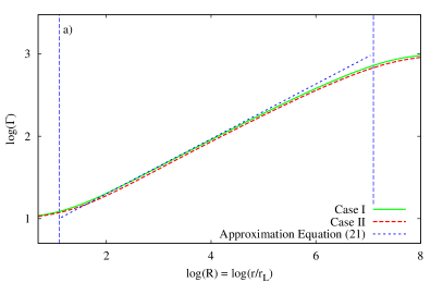
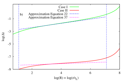
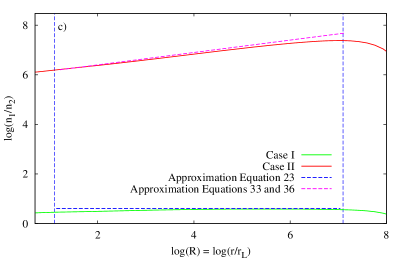
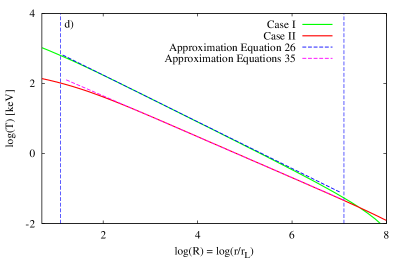
Figure 2: From top left to bottom right, radial evolution of the Lorentz factor $\Gamma$, of the current sheet width $\Delta$, of the ratio of densities $n_{1}^{{}^{\prime}}/n_{2}^{{}^{\prime}}$, and of the temperature $T^{{}^{\prime}}$. The blue and purple dashed lines represent the approximations derived in Section 3. Finally, the vertical blue dashed lines represent $R_{0,\rm I}$ and $R_{\rm c,\rm I}$. For clarity, we do not display the corresponding value for case II as they are respectively close to $R_{0,\rm I}$ and $R_{\rm c,\rm I}$.

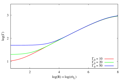
Figure 3: Radial evolution of the Lorentz factor for initial conditions $\Gamma_{0}=10,20,50$ and same $\Gamma_{\rm max}$ in case II. After a transition corresponding to adjustments from the initial conditions, all evolutions follow the asymptote given by Equation 30.

4 Transitions radii in the striped wind scenario

4.1 The photospheric radius

The derivations presented above are valid as long as the radiation and matter are strongly coupled, namely below the photosphere. In calculating the photospheric radius, one can use the general expression of the optical depth for a photon emitted at radius $r$ on the line of sight first derived by Abramowicz et al. (1991),

$$\tau(r)=\sigma_{\rm T}\int_{R}^{\infty}\Gamma n^{{}^{\prime}}(1-\beta)ds.$$ (38)

Here, $\sigma_{\rm T}$ is the Thompson cross-section, and the integration is performed over the photon path. In deriving the analytical expression below, we assume that the photospheric radius is below the coasting radius, namely $r_{\rm ph}/r_{L}<R_{\rm c,I,II}$. As we show below, this is the case for parameters characterizing GRB outflow. The contribution of the current sheet to the total opacity can be neglected since only a small fraction of the matter is contained in the current sheet during the accelerating phase. Using first order expansion $(1-\beta)\simeq 1/(2\Gamma^{2})$ one finds

$$\tau(r)=\sigma_{T}\frac{\Gamma_{0}R_{0,i}^{2}n_{0,i}^{{}^{\prime}}}{2\mathcal{A}_{i}}\frac{3}{5r^{\frac{5}{3}}},$$ (39)

where the index $i={\rm I,II}$ for the two cases considered above. Furthermore, in case I, $\mathcal{A}_{i}\equiv\mathcal{A}_{\rm I}=(5A\Gamma_{\rm max})^{\frac{2}{3}}$, while in case II, $\mathcal{A}_{i}\equiv\mathcal{A}_{\rm II}=\left(30A\Gamma_{\rm max}/7\right)^{\frac{2}{3}}$. The photospheric radius is, by definition, the radius at which $\tau(r_{\rm ph})=1$, from which one finds

$$r_{\rm ph} =\left[\frac{3\sigma_{\rm T}\Gamma_{0}R_{0,i}^{2}n_{0,i}^{{}^{\prime}}}{10\mathcal{A}_{i}}\right]^{\frac{3}{5}}=\left\{\begin{array}[]{l l}6.8\times 10^{11}~{}L_{52}^{\frac{3}{5}}(\epsilon\Omega)_{3}^{-\frac{2}{5}}\Gamma_{\rm max,3}^{-1}{\rm~{}cm}&{\rm case~{}I,}\\ 7.0\times 10^{11}~{}L_{52}^{\frac{3}{5}}(\epsilon\Omega)_{3}^{-\frac{2}{5}}\Gamma_{\rm max,3}^{-1}{\rm~{}cm}&{\rm case~{}II}.\end{array}\right.$$ (42)

Here and below, $X=10^{n}X_{n}$ in cgs units. We thus conclude that the difference between the photospheric radii is small, as it is mainly due to the difference in the Lorentz factor. Since the parametric dependence is the same in both cases, we drop the distinction between case I and case II when referring to the photospheric radius from here on. In addition, the photospheric radius is almost two orders of magnitude smaller than the coasting radius for the fiducial parameters of our model.

4.2 Transition between the regimes I and II

We considered the flow in two cases: (I) the radiation is locked in the current sheet and (II) the radiation escapes freely the current sheet filling the whole space. Applying our results to GRBs, we now check when our assumptions are valid.

In case I, the key assumption is that photons remain in the current sheet. It requires that the rate of diffusion through the current sheet be small. This condition ceases to be fulfilled at the radius $r_{\rm D,I}^{\Delta}$ above which radius, diffusion through the current sheet is efficient. When Compton scattering dominates, the diffusion time through the current sheet is given by

$$t_{\rm D}^{\Delta}=\frac{\sigma_{T}n_{1}^{{}^{\prime}}(\Gamma\Delta l_{0})^{2}}{2c},$$ (43)

while the diffusion time through the magnetized region is obtained by replacing $\Delta$ by $1-\Delta$. Equating the diffusion time to the expansion time $t_{\rm exp}=r/\Gamma c$ gives for the current sheet

$$r_{\rm D,I}^{\Delta} =6.05\times 10^{10}~{}L_{52}^{\frac{3}{5}}(\epsilon\Omega)_{3}^{\frac{4}{5}}l_{0,7}^{\frac{6}{5}}\Gamma_{\rm max,3}^{-1}{\rm~{}cm}.$$ (44)

Above $r_{\rm D,I}^{\Delta}$, energy leaves the current sheet, taking away heat and entropy, which are (partially) redistributed in the magnetized region by Compton scattering, since $r_{\rm D,I}^{\Delta}<r_{\rm ph}$.

Case II is defined by two conditions. First, it is assumed that the energy deposited by reconnection in the current sheet can be redistributed in the magnetized region. It implies that diffusion through the current sheet is efficient. Second, the temperature in the current sheet and in the magnetized region are assumed to be similar $T_{1}^{{}^{\prime}}\sim T_{2}^{{}^{\prime}}$, such that the pressure balance condition is satisfied by the gas pressure rather than the radiation pressure. We point out that in practice because energy is continuously deposited by reconnection in the current sheet, the average temperature of the current sheet $\bar{T}_{1}^{{}^{\prime}}$ is always larger than the average temperature in the magnetized region $\bar{T}_{2}^{{}^{\prime}}$, as long as the opacity of the current sheet be larger than the unity. Still for $T_{1}^{{}^{\prime}}\gtrapprox T_{2}^{{}^{\prime}}$ at the boundary of the current sheet, $\Delta p_{\rm g}\gg\Delta p_{\rm rad}$, and the conditions for case II are satisfied.

In the regime II, the plasma density in the current sheet is so high that the free-free absorption/emission becomes important. Using the Rosseland mean for free-free emission $\alpha_{\rm R}^{\rm ff}$, given by Equation 5.20 of Rybicki & Lightman (1979), the ratio of free-free opacity to photon scattering opacity is given by

$$\frac{\alpha_{\rm R}^{\rm ff}}{\sigma_{T}n_{e}^{{}^{\prime}}}=0.24~{}\Gamma_{\rm max,3}^{\frac{5}{6}}(\epsilon\Omega)_{3}^{-\frac{7}{24}}r^{-\frac{1}{24}}L_{52}^{-\frac{1}{8}}.$$ (45)

One sees that the free-free opacity remains less than the scattering opacity, the photon diffusion time is determined by the Thomson scattering. However, free-free absorption/emission efficiently thermalized radiation provided the condition

$$\sqrt{\alpha^{\rm ff}_{\rm R}\sigma_{T}n^{\prime}_{e}}\Delta\Gamma l_{0}>1,$$ (46)

is fulfilled (Shakura, 1972). Substituting the parameters of the flow, one finds that the radiation from the current sheet is thermalized up to the distance

$$r^{\Delta}_{\rm ff,II}=2.2\times 10^{11}L_{52}^{\frac{5}{9}}(\epsilon\Omega)_{3}^{\frac{1}{9}}l_{0,7}^{\frac{16}{27}}\Gamma_{\rm max,3}^{-\frac{20}{27}}{\rm~{}cm}.$$ (47)

In the context of GRB, this might have profound effects on the emitted spectrum at the photosphere. In particular, it has the potential of solving the soft photon problem (see section 5.2 below). A detailed analysis of photon production and Comptonization below the photosphere in the striped wind scenario is out of the scope of the current paper, but it will be presented in a future publication.

Above this radius, the condition for case II, namely efficient energy diffusion through the current sheet is satisfied. We mention that for equal average temperatures, $\bar{T}_{1}^{{}^{\prime}}\sim\bar{T}_{2}^{{}^{\prime}}$, one also needs to require efficient diffusion through the magnetized region. This condition is satisfied above the radius

$$r_{\rm D,II}^{1-\Delta}=8.0\times 10^{11}~{}L_{52}^{\frac{3}{7}}l_{0,7}^{\frac{6}{7}}(\epsilon\Omega)^{\frac{2}{7}}\Gamma_{\rm max,3}^{-\frac{1}{7}}{\rm~{}cm}$$ (48)

obtained by using Equation 43 with $\Delta\rightarrow 1-\Delta$. We point out that $r_{\rm D,II}^{1-\Delta}>r_{\rm ph}$, above which Compton scattering ceases. Therefore, the energy is never fully homogenized in the magnetized region.

In the above computations, we presented two limiting cases: case I in which the radiation is locked in the current sheet, and case II, in which radiation can stream efficiently through the current sheet. At the formation of the reconnection layer, radiation is always trapped inside of it. Below the diffusion radius $r_{\rm D,I}^{\Delta}$, given by Equation 44, radiation remains in the current sheet. Therefore, the dynamics follows the limiting case I until this radius.

Only at radii $r>r_{\rm D,I}^{\Delta}$, energy can diffuse through the reconnection layer, and the contribution of radiation to the pressure balance condition decreases. As a result, the current sheet shrinks and its density increases. At $r_{\rm D,I}^{\Delta}$, the opacity of the current sheet is larger than the unity for parameters characterizing limiting case II. It implies that the average temperature of the current sheet $\bar{T}_{1}^{{}^{\prime}}$ is larger than the temperature of the magnetized region $\bar{T}_{2}^{{}^{\prime}}$ at these radii. Yet, because the temperature is weakly dependent on the optical depth, with $T^{{}^{\prime}}\propto\tau^{1/4}$, one could expect that the dynamics will not be significantly modified. Moreover, as it was shown above, the radiation energy density within the magnetized region remains inhomogeneous, contrary to the assumptions of the case II. This means that our case II may be considered as an idealized limiting case. But taking into account that the dynamics of the flow is nearly the same on the limiting cases I and II, one can be sure that it remains the same even in the intermediate case.

5 Discussion

5.1 Dynamics

We find that the acceleration of the outflow is very similar in limiting cases I and II. The radial evolution of the Lorentz factor is mostly due to our choice of reconnection rate, given by Equation 10. It constitutes the main assumption of our work. As already pointed out, when studying pulsar wind nebulae, Coroniti (1990) and Lyubarsky & Kirk (2001) parametrize the width of the reconnection layer $\Delta$ by its proportionality with the Larmor radius, such that $\Delta\Gamma l_{0}=\kappa k_{\rm B}T^{{}^{\prime}}_{1}/(e\mathcal{B}^{{}^{\prime}})$, where $\kappa$ is a constant in the order of the unity. The main difference with the GRB scenario is the important baryon load expected from the progenitor, see e.g. Levinson & Eichler (2003). In fact, reconnection happens when the charge density in the current sheet cannot sustain the required current (Usov, 1975), which in the context of GRBs happens only at very large radius.

The micro-physical details of reconnection happen on the length-scale of few tens of plasma skin depth (Sironi & Spitkovsky, 2014). Comparing the comoving sheet width and the plasma skin depth $\Lambda$ of the current sheet at the photosphere, we find for case II:

$$l_{\rm cs}=\Delta l_{0}\Gamma =66~{}L_{52}^{\frac{1}{2}}l_{0,7}(\epsilon\Omega)_{3}^{\frac{3}{4}}\Gamma_{\rm max,3}^{-\frac{7}{4}}{~{}~{}\rm cm,}$$ (49)

$$\Lambda=\frac{c}{\sqrt{\frac{4\pi n^{{}^{\prime}}_{1}e^{2}}{m_{p}}}} =2.2\times 10^{-4}~{}L_{52}^{\frac{1}{4}}\Gamma_{\rm max,3}^{-\frac{7}{8}}(\epsilon\Omega)_{3}^{-\frac{1}{8}}{~{}~{}\rm cm.}$$ (50)

It is readily checked that $l_{\rm cs}\gg\Lambda$ at every radii. A similar result holds for case I as well. This result therefore implies that the evolution of the striped wind is described by a macro-physical rather than micro-physical process.

Spruit et al. (2001) postulated the reconnection rate as given by Equation 10, assuming that the alternating magnetic field annihilates with a rate close to $\sim 0.1$ of the Alfvén speed, which is comparable to the speed of light in highly magnetized outflows. Later, Lyubarsky (2010) justified this assumption by showing that the reconnection is triggered by the self-sustained Kruskal-Schwarzschild instability. This instability makes the plasma “drips out” of current sheets as a result of its own acceleration, favouring the field reconnection and maintaining the plasma acceleration, hence the self-sustained characteristic of the instability. In the context of GRBs, reconnection is therefore the result of a macro-physical MHD instability.

The MHD instabilities will eventually destroy the striped wind. This process was studied by Zrake (2016) in the context of pulsar winds under the guise of force-free electrodynamics. In this work, it was found that the plasma instabilities become dominant once the causal contact is established between the stripes, which happens after a comoving fast magnetosonic time. The characteristic radius at which this happens, $r_{\rm tur}$, can be calculated by comparing the comoving expansion time $r/(\Gamma c)$ to the crossing time of a stripe by a fast magnetosonic wave, $\Gamma l_{0}/(\beta_{\rm fms}c)$, where $\beta_{\rm fms}$ is the speed of the fast magnetosonic wave, associated with the Lorentz factor $\Gamma_{\rm fms}=(\sigma_{0}\Gamma_{0}/\Gamma)^{1/2}$. Assuming $\beta_{\rm fms}\sim 1$ and case I, one obtains ${r_{\rm tur}=7.1\times 10^{11}l_{0,7}^{3}(\epsilon\Omega)_{3}^{2}\Gamma_{\rm max,3}^{2}}$cm, close to the photospheric radius. Note the very strong dependence on the parameters, and especially on $l_{0}$. The turbulence is fully established and developed after a time four times longer than it takes the fast magnetosonic wave to cross one stripe (Zrake, 2016). It corresponds to the radius $r=4.5\times 10^{13}l_{0,7}^{3}(\epsilon\Omega)_{3}^{2}\Gamma_{\rm max,3}^{2}$cm.

Finally, we note that if all the magnetic energy were to be transformed to kinetic energy, the maximum Lorentz factor achieved by the outflow would be $\Gamma_{\rm max}=\sigma_{0}\Gamma_{0}$. However, under the assumption of high radiative efficiency, Drenkhahn & Spruit (2002) explained that a large fraction of the total energy is carried away by radiation, substantially reducing the final Lorentz factor. It was recently shown by Pe’er (2016) that up to half of the total energy can be emitted, reducing the final Lorentz factor down to $\Gamma_{\rm max}/2$. In this paper, we discarded this effect as we were interested in the solution below the photosphere, where coupling between the radiation and particles is efficient, as required by our assumptions. A detailed description of the spectrum emitting at the photosphere and at larger radii will be given in a future work.

5.2 Implications for the prompt emission of GRBs

The observed MeV peak energy in the spectrum of the prompt GRB emission can be attributed to thermalization processes inside the photosphere of the outflow (Eichler & Levinson, 2000; Mészáros & Rees, 2000; Rees & Mészáros, 2005; Thompson et al., 2007; Beloborodov, 2013; Vurm et al., 2013). This requires models of sub-photospheric dissipation to be able to produce photons efficiently. Indeed, in a scenario in which photons cannot be produced and if dissipation occurs, the photons already present in the outflow would share the dissipated energy. As their average comoving energy is strongly increased, the observed spectral peak energy is shifted to large values. Assuming a luminosity-peak energy correlation, also referred to as Yonetoku correlation (Yonetoku et al., 2004), Beloborodov (2013) and Vurm et al. (2013) found that the Lorentz factor of GRBs can not be larger than $\sim 10$ at the dissipation radius. This analysis is based on photon production processes, necessary to achieve thermalization and regulate the energy of the thermal peak. This result holds independently of both the content (baryonic, magnetic and thermal) and of the acceleration mechanism of the plasma, still unknown and highly debated (Zhang & Pe’er, 2009; Bromberg et al., 2015; Bégué & Pe’er, 2015).

Referring to the striped wind scenario, Vurm et al. (2013) also considered the Bremsstrahlung rate when the plasma is clumped, i.e. when over-dense regions exist. Indeed, because Bremsstrahlung depends on the density square, compressed regions could play an important role in producing photons. Yet, they had to assume the fraction of energy carried by Poynting flux. They further estimated the compression ratio to be around $10^{6}$ by satisfying the pressure balance condition with the gas pressure. In this paper, we consistently obtained the compression ratio, based on first principle MHD, and find that it agrees with the estimate of Vurm et al. (2013) for case II.

In case I, the compression ratio is small, being only 4. Therefore, the Bremsstrahlung process is not expected to be much more efficient than if no matter clumping was present. Using the same procedure as in Vurm et al. (2013) and Beloborodov (2013), we find that Bremsstrahlung freezes out at radius

$$\bar{r}_{\rm ff,I}^{\Delta} =8.0\times 10^{8}~{}\left(\frac{\bar{A}}{15}\right)^{\frac{3}{5}}L_{52}^{\frac{27}{40}}\Gamma_{\rm max,3}^{-\frac{29}{20}}(\epsilon\Omega)_{3}^{-\frac{1}{4}}~{}\text{cm,}$$ (51)

where $\bar{A}$ depends weakly on the temperature and is found to be nearly constant (Bégué & Pe’er, 2015). This result is compatible with that of Vurm et al. (2013) and Beloborodov (2013). We note that in this situation, the outflow is unable to sustain the thermalization of the plasma as photons cannot be created (unless the outflow remains relatively slow with $\Gamma\sim 10$ at radius $r\sim 10^{10}$cm). Therefore, the emission of such an outflow is characteristic of the photon starvation scenario discussed in Bégué & Pe’er (2015).

In case II however, the compression ratio is very large $\sim 10^{6}$ (as required by the pressure balance condition). As a result, Bremsstrahlung photon production is efficient at least up to $r_{\rm ff,II}^{\Delta}$ given by 47, which implies that the radiation from the current sheet be thermalized almost up to the photosphere.

6 Conclusion

In this paper, we presented a detailed analysis of the effects of radiation on the striped wind model. In the context of GRBs, this is required as the wind is initially optically thick due to the large baryon load. Previous studies of the dynamics of the striped wind model in the context of GRBs (Drenkhahn & Spruit, 2002; Drenkhahn, 2002) discarded the internal structure of the wind, preventing to study how radiation effects the dynamics of the plasma and its internal structure.

We presented an analytic asymptotic solution to the relativistic magneto-hydrodynamics equations by employing the short-wavelength approximation initially developed in Lyubarsky & Kirk (2001). The solution depends on whether or not radiation can diffuse through the current sheet. Yet, the difference in the evolution of the Lorentz factor between the two limiting scenarios is small, and only the current sheet width and density are substantially modified.

We explained that case I is initially relevant for wind parameters compatible with GRB physics. Above $r_{\rm D,I}^{\Delta}$, photons in the current sheet diffuse into the magnetized region. As a result, the radiation pressure of the current sheet drops, implying a decrease of its width, while its density increases to compensate for the magnetic pressure. Once this happens, the dynamics transitions to the case II scenario. The rate of photon production by the free-free process increases, implying that the current sheet be thermalized up to $\sim 10^{11}$cm, slightly smaller than the photosphere. This effect could provide a solution to the soft photon problem in GRBs.

To conclude, our results pave the way for studies dedicated to the effects of radiation on the dynamical evolution of a striped wind.

Appendix A Relativistic radiative MHD equations of the striped wind

The relativistic radiation hydrodynamics equations in spherical coordinates are given by e.g. Park (2004). In this appendix, the expressions are directly specialised to spherical symmetry, namely $\partial/\partial\theta=\partial/\partial\phi=0$. In the context of the striped wind, the stress energy tensor can be divided into its matter and field components, $T=T_{\rm g}+T_{\rm M}$. The stress energy tensor of an ideal gas is $T_{g}^{\mu\nu}=h_{\rm g}U^{\mu}U^{\nu}+p_{\rm g}g^{\mu\nu}$. Here, $U^{\mu}=(\Gamma,\Gamma v,0,0)$ is the 4-velocity, $\Gamma$ and $v$ are the Lorentz factor of the flow and the speed, $p_{\rm g}$ is the gas pressure, $h_{\rm g}=\epsilon_{\rm g}+p_{\rm g}$ is the proper gas enthalpy, and its proper energy density is $\epsilon_{\rm g}$. Finally, $g^{\mu\nu}$ is the Minkowski metric tensor.

The electro-magnetic component of the plasma is described by the electro-magnetic stress-energy tensor $T_{\rm M}^{\alpha\beta}=(1/4\pi)(F^{\alpha\gamma}F^{\beta}_{~{}\gamma}-(1/4)g^{\alpha\beta}F_{\gamma\nu}F^{\gamma\nu})$, where $F^{\alpha\beta}$ is the Maxwell field tensor. In the context of the striped wind, far from the light-cylinder $r_{\rm L}$, the laboratory frame magnetic field is toroidal $\vec{\mathcal{B}}=\mathcal{B}(r,t)\vec{\phi}$. It implies that the laboratory frame electric field and current density are $\vec{\mathcal{E}}=\mathcal{E}(r,t)\vec{\theta}$ and $\vec{j}=j(r,t)\vec{\theta}$. The only non-null components of the Maxwell tensor are $F^{02}=r\mathcal{E}$, $F^{12}=-r\mathcal{B}$, $F^{20}=-r\mathcal{E}$ and $F^{21}=r\mathcal{B}$.

The radiation stress energy tensor is $R^{\mu\nu}=\iint I(\vec{n},\nu)n^{\mu}n^{\nu}d\nu d\Omega$, where $I$ is the specific intensity of photons of frequency $\nu$ moving in the direction $\vec{n}$. We further assume that radiation is isotropic in the comoving frame. It implies that all the only non-vanishing components of $R^{\mu\nu}$ are on the diagonal, when it is expressed in the comoving frame. In addition, ${\rm diag}(R^{\mu\nu})=(\epsilon_{\rm rad}^{{}^{\prime}},P^{{}^{\prime}}_{\rm rr},P^{{}^{\prime}}_{\theta\theta},P^{{}^{\prime}}_{\phi\phi})$ where $\epsilon_{\rm rad}^{{}^{\prime}}$ is the comoving energy density in radiation, and $P^{{}^{\prime}}_{\rm rr}=P^{{}^{\prime}}_{\theta\theta}=P^{{}^{\prime}}_{\phi\phi}=\epsilon_{\rm rad}^{{}^{\prime}}/3$.

The number density conservation $(nU^{\alpha})_{;\alpha}$ becomes

$$\frac{\partial}{\partial t}(\Gamma n^{{}^{\prime}})+\frac{1}{r^{2}}\frac{\partial}{\partial r}(r^{2}n^{{}^{\prime}}v\Gamma)=0.$$ (52)

By noting $G^{\mu}$ the radiation 4-force density, further assuming that there is no external force, the Bianci identity for the radiation on the one hand and matter plus magnetic component on the other hand can be separated. It comes

$$T^{\mu\nu}_{~{}~{};\nu} =G^{\mu} \text{matter and electromagnetic field},$$ (53)

$$R^{\mu\nu}_{~{}~{};\nu} =-G^{\mu}$$ radiation. (54)

The energy equation is the zeroth component of the divergence of the stress energy tensor

$$\frac{\partial}{\partial t}\left(T^{00}\right)+\frac{1}{r^{2}}\frac{\partial}{\partial R}\left(r^{2}T^{01}\right)=G^{0},$$ (55)

where $G^{0}$ is the zeroth component of the radiation four-force. With $T^{00}_{\rm M}=(\mathcal{E}^{2}+\mathcal{B}^{2})/(8\pi)$ and $T_{\rm M}^{01}=c\mathcal{E}\mathcal{B}/(4\pi)$, the energy equation reduces to

$$\frac{\partial}{\partial t}\left(h_{\rm g}^{{}^{\prime}}\Gamma^{2}-p_{\rm g}\right)+\frac{1}{r^{2}}\frac{\partial}{\partial r}\left(r^{2}v\Gamma^{2}h_{\rm g}^{{}^{\prime}}\right)+\frac{\partial}{\partial t}\left(\frac{\mathcal{E}^{2}+\mathcal{B}^{2}}{8\pi}\right)+\frac{1}{r^{2}}\frac{\partial}{\partial r}\left(r^{2}\frac{\mathcal{EB}c}{4\pi}\right)=G^{0}.$$ (56)

The entropy equation is obtained by projecting Equation 53 along $U_{\mu}$ and by using ${T^{\mu\nu}_{M~{};\nu}=-F^{\mu}_{~{}l}J^{l}}$, where $J=(cqn,0,j,0)^{\rm T}$ is the four-current. The equation can be simplified to:

$$-n^{{}^{\prime}}\Gamma\frac{\partial}{\partial t}\left(\frac{h^{{}^{\prime}}_{\rm g}}{n^{{}^{\prime}}}\right)-n^{{}^{\prime}}\Gamma v\frac{\partial}{\partial r}\left(\frac{h^{{}^{\prime}}_{\rm g}}{n^{{}^{\prime}}}\right)+\Gamma\frac{\partial}{\partial t}\left(p_{\rm g}\right)+\Gamma v\frac{\partial}{\partial r}\left(p_{\rm g}\right)=j\Gamma(\mathcal{E}-\frac{v}{c}\mathcal{B})-\Gamma G^{\rm 0}+\Gamma vG^{\rm 1},$$ (57)

where we used Equation 52 to simplify the terms in $r^{2}$. In the absence of radiation ($G^{0}=G^{1}=0$), when specializing to the equation of state $p_{g}=(\hat{\gamma}-1)(\epsilon_{g}-n^{{}^{\prime}}mc^{2})$, where $\hat{\gamma}$ is the adiabatic index of the gas and $c$ the speed of light, one recovers the entropy equation A4 of Lyubarsky & Kirk (2001):

$$\frac{1}{\hat{\gamma}-1}\left[\frac{\text{d}}{\text{d}t}p_{\rm g}-\frac{\hat{\gamma}p_{\rm g}}{n^{{}^{\prime}}}\frac{\text{d}}{\text{d}t}n^{{}^{\prime}}\right] =j(\mathcal{E}-\frac{v}{c}\mathcal{B}),$$ (58)

where the convective derivative is

$$\frac{\text{d}}{\text{d}t}=\frac{\partial}{\partial t}+v\frac{\partial}{\partial r}.$$ (59)

We now turn to express the conservation equation for the radiation. In the laboratory frame the radiation stress energy tensor becomes

$$R^{\mu\nu}=\left(\begin{tabular}[]{cccc}$\hbox{}\epsilon_{\rm rad}=\frac{4}{3}\Gamma^{2}\epsilon_{\rm rad}^{{}^{\prime}}-\frac{\epsilon_{\rm rad}^{{}^{\prime}}}{3}$&$F^{\rm r}=\frac{4}{3}\Gamma^{2}v\epsilon_{\rm rad}^{{}^{\prime}}$&$0$&$0$\\ $\hbox{}F^{\rm r}$&$P_{\rm rr}=\left(\frac{4}{3}\Gamma^{2}-1\right)\epsilon_{\rm rad}^{{}^{\prime}}$&$0$&$0$\\ $\hbox{}0$&$0$&$P_{\rm\theta\theta}=P^{{}^{\prime}}_{\rm\theta\theta}$&$0$\\ $\hbox{}0$&0&0&$P_{\rm\phi\phi}=P_{\rm\phi\phi}^{{}^{\prime}}$\end{tabular}\right).$$ (64)

The radiation energy equation is obtained by taking the zeroth component of the divergence of the radiation stress energy tensor

$$\frac{\partial}{\partial t}\left(\epsilon_{\rm rad}\right)+\frac{1}{r^{2}}\frac{\partial}{\partial r}\left(r^{2}F^{\rm r}\right)=-G^{0},$$ (65)

while the radiation momentum equation is obtained from the first component of the divergence of the radiation stress energy tensor

$$\frac{\partial}{\partial t}\left(F^{\rm r}\right)+\frac{\partial}{\partial r}\left(P_{\rm rr}\right)+\frac{8}{3}(\Gamma^{2}-1)\frac{\epsilon_{\rm rad}^{{}^{\prime}}}{r}=-G^{1}.$$ (66)

These two equations give the expression of the radiation four-force appearing in Equations 56 and 57.

The system is completed by Maxwell’s equations. Ampere’s law reads

$$\frac{1}{r}\frac{\partial}{\partial r}\left(r\mathcal{B}\right)+\frac{1}{c}\frac{\partial}{\partial t}\left(\mathcal{E}\right)+\frac{4\pi}{c}j=0.$$ (67)

Faraday’s law is

$$\frac{1}{r}\frac{\partial}{\partial r}\left(r\mathcal{E}\right)+\frac{1}{c}\frac{\partial}{\partial t}\left(\mathcal{B}\right)=0,$$ (68)

and Ohm’s law

$$j=\sigma_{c}\gamma\left(\mathcal{E}-\frac{v}{c}\mathcal{B}\right).$$ (69)

Here $\sigma_{\rm c}$ is the conductivity of the plasma. The system is closed by the ideal gas law and an equation of state:

$$p_{\rm g} =k_{\rm B}n^{{}^{\prime}}T^{{}^{\prime}},$$ (70)

$$p_{\rm g} =(\hat{\gamma}-1)(\epsilon_{g}-n^{{}^{\prime}}mc^{2}).$$ (71)

Appendix B Perturbative approach to the MHD equations: decomposition into fast and slow variables

Here, we follow similar steps to the mathematical derivation of Lyubarsky & Kirk (2001). The problem at hand naturally possesses two time scales. On the one hand, the rotation period of the pulsar defines the fast time-scale $t_{\rm f}=2\pi/\Omega$. We further assume that at a distance of a few light-cylinder radii from the central compact object, the pattern of the wind (which consists of the current sheet and the magnetized region) is stationary. The speed of the flow does not change within one pattern, while magnetic field, density, pressure and radiation vary internally (between the hot and cold layers). The system can therefore be thought as an entropy wave comoving with the fluid. This wave evolves on a slow time scale corresponding to the expansion time of the wind $t_{\rm s}\sim 2\pi r/(r_{L}\Omega)$. Following Lyubarsky & Kirk (2001), the procedure we follow is (1) transform the problem to the slow and fast independent variables, (2) expand the parameters, (3) solve for the zeroth order equations, (4) solve the first order equations requiring that the secular terms they contain vanish.

We first define the phase (over one pattern)

$$\Phi=\Omega\left[t-\int_{0}^{r}\frac{dr^{{}^{\prime}}}{v_{w}(r^{{}^{\prime}})}\right],$$ (72)

where $v_{w}(r)$ is the speed of the pattern, which will be determined later. Then, the coordinates of the problem are changed from $(r,t)$ to $(R,\Phi)$ where $R=\epsilon r/r_{L}$, with $\epsilon\ll 1$ and $R\sim 1$. The Jacobian of the transformation is

$$\mathcal{J}=\left(\begin{tabular}[]{cc}$\hbox{}\frac{\partial}{\partial t}\left(\Phi\right)=\Omega$&$\frac{\partial}{\partial t}\left(R\right)=0$\\ $\hbox{}\frac{\partial}{\partial r}\left(\Phi\right)=-\frac{\Omega}{v_{\omega}}$&$\frac{\partial}{\partial r}\left(R\right)=\frac{\epsilon}{r_{L}}$\end{tabular}\right).$$ (75)

The continuity equation in the new set of coordinates is

$$\frac{\partial}{\partial\Phi}\left(\Gamma n^{{}^{\prime}}\right)-\frac{1}{v_{w}}\frac{\partial}{\partial\Phi}\left(\Gamma\beta n^{{}^{\prime}}\right)+\frac{\epsilon}{cR^{2}}\frac{\partial}{\partial R}\left(R^{2}\Gamma vn^{{}^{\prime}}\right)=0,$$ (76)

where the definition of the light-cylinder was used, $r_{\rm L}=c/\Omega$. The energy equation 55 gets the form

$$\Omega\frac{\partial}{\partial\Phi}\left(T^{00}+\epsilon_{\rm rad}\right)+\frac{1}{R^{2}}\frac{\epsilon}{r_{L}}\frac{\partial}{\partial R}\left(R^{2}(T^{01}+F^{r})\right)-\frac{\Omega}{v_{w}}\frac{\partial}{\partial\Phi}\left(T^{01}+F^{r}\right)=0,$$ (77)

where Equation 65 was used to express $G^{0}$. Transforming the entropy Equation 57 is more cumbersome, and after long but simple substitution algebra, it becomes

$$~{}~{}\left[\hat{\gamma}p_{\rm g}+(\hat{\gamma}-1)h_{\rm rad}^{{}^{\prime}}\right]\frac{\partial}{\partial\Phi}\left(\Gamma\right)+\Gamma\frac{\partial}{\partial\Phi}\left(p_{\rm g}+\frac{3}{4}(\hat{\gamma}-1)h_{\rm rad}^{{}^{\prime}}\right)-\frac{\hat{\gamma}p_{\rm g}+(\hat{\gamma}-1)h_{\rm rad}^{{}^{\prime}}}{v_{w}}\frac{\partial}{\partial\Phi}\left(v\Gamma\right)$$

$$- ~{}~{}\frac{\Gamma v}{v_{w}}\frac{\partial}{\partial\Phi}\left(p_{\rm g}+\frac{3}{4}(\hat{\gamma}-1)h_{\rm rad}^{{}^{\prime}}\right)+\frac{\epsilon}{cR^{2}}\left[\hat{\gamma}p_{\rm g}+(\hat{\gamma}-1)h_{\rm rad}^{{}^{\prime}}\right]\frac{\partial}{\partial R}\left(R^{2}\Gamma v\right)$$

$$+ ~{}~{}\frac{\epsilon\Gamma v}{c}\frac{\partial}{\partial R}\left(p_{\rm g}+\frac{3}{4}(\hat{\gamma}-1)h_{\rm rad}^{{}^{\prime}}\right)=\frac{\hat{\gamma}-1}{\Omega}\Gamma(\mathcal{E}-\frac{v}{c}\mathcal{B})j,$$ (78)

where the radiation enthalpy $h_{\rm rad}^{{}^{\prime}}=4\epsilon_{\rm rad}^{{}^{\prime}}/3$. Finally, the Ampere’s and Faraday’s equation becomes

$$\frac{\partial}{\partial\Phi}\left(\mathcal{E}\right)-\frac{c}{v_{w}}\frac{\partial}{\partial\Phi}\left(\mathcal{B}\right)+\frac{\epsilon}{R}\frac{\partial}{\partial R}\left(R\mathcal{B}\right)+\frac{4\pi}{\Omega}j =0,$$ (79)

$$\frac{\partial}{\partial\Phi}\left(\mathcal{B}\right)-\frac{c}{v_{\omega}}\frac{\partial}{\partial\Phi}\left(\mathcal{E}\right)+\frac{\epsilon}{R}\frac{\partial}{\partial R}\left(R\mathcal{E}\right) =0.$$ (80)

In order to simplify the equations, we introduce $\beta=v/c$ and $\beta_{\omega}=v_{\omega}/c$. We further expand all the quantities to the first order in $\epsilon$ such that for a quantity $\mathcal{X}$, we write ${\mathcal{X}=\mathcal{X}_{0}(\Phi,R)+\epsilon\mathcal{X}_{1}(\Phi,R)}$. Since an entropy wave is considered, we have $\partial\beta_{0}/\partial\Phi=0$.

Expanding the continuity equation in $\epsilon$, the zeroth order gives $\beta_{\omega}=\beta_{0}(R)$. Therefore, using Ampere and Faraday equations gives

$$\frac{\partial}{\partial\Phi}\left(\mathcal{B}_{0}\right) =\frac{4\pi\Gamma_{0}^{2}\beta_{0}}{\Omega}j_{0}.$$ (81)

Faraday Equation 80 implies that $\mathcal{E}_{0}-\beta_{0}\mathcal{B}_{0}$ is independent of $\Phi$. In the region where the assumption of ideal MHD holds, Ohm’s law imposes

$$\mathcal{E}_{0} =\beta_{0}\mathcal{B}_{0}.$$ (82)

At the zeroth order in $\epsilon$, the energy Equation 77 simplifies to

$$\frac{\partial}{\partial\Phi}\left(p_{\rm g,0}+\frac{\mathcal{B}_{0}^{2}}{8\pi\Gamma_{0}^{2}}+\frac{\epsilon_{\rm rad,0}^{{}^{\prime}}}{3}\right)=0$$ (83)

which is the pressure balance condition of the current sheet. In addition, it is immediately checked that the entropy equation is satisfied at the zeroth order in $\epsilon$.

In order to describe the internal structure, one needs to consider the first order in $\epsilon$. In this order, the continuity equation becomes

$$\frac{\Gamma_{0}}{\beta_{0}}\frac{\partial}{\partial\Phi}\left(\beta_{1}n_{0}^{{}^{\prime}}\right)=\frac{1}{R^{2}}\frac{\partial}{\partial\Phi}\left(R^{2}\Gamma_{0}\beta_{0}n_{0}^{{}^{\prime}}\right),$$ (84)

and the two Maxwell equations

$$\frac{\partial}{\partial\Phi}\left(\mathcal{E}_{1}-\frac{\mathcal{B}_{1}}{\beta_{0}}\right) =-\frac{1}{R}\frac{\partial}{\partial\Phi}\left(R\mathcal{B}_{0}\right)-\frac{4\pi}{\Omega}j_{1},$$ (85)

$$\frac{\partial}{\partial\Phi}\left(\mathcal{B}_{1}-\frac{\mathcal{E}_{1}}{\beta_{0}}\right) =-\frac{1}{R}\frac{\partial}{\partial\Phi}\left(R\beta_{0}\mathcal{B}_{0}\right).$$ (86)

Ohm’s law reads

$$j_{1}=\sigma_{\rm c}[\Gamma_{1}(\mathcal{E}_{0}-\beta_{0}\mathcal{B}_{0})+\Gamma_{0}(\mathcal{E}_{1}-\beta_{0}\mathcal{B}_{1})-\Gamma_{0}\beta_{1}\mathcal{B}_{0}].$$ (87)

The first term is null according to the zeroth order Ohm’s law together with the assumption of ideal MHD. One therefore obtains

$$\mathcal{E}_{1}=\beta_{0}\mathcal{B}_{1}+\beta_{1}\mathcal{B}_{0}.$$ (88)

Using Equation 88 in the Faraday Equation 86 leads to

$$\frac{\partial}{\partial\Phi}\left(\frac{\beta_{1}}{\beta_{0}}\mathcal{B}_{0}\right)=\frac{1}{R}\frac{\partial}{\partial R}\left(R\beta_{0}\mathcal{B}_{0}\right).$$ (89)

Dividing both sides of this last equation by $R^{2}\beta_{0}\Gamma_{0}n_{0}^{{}^{\prime}}$, multiplying both sides of Equation 84 by $\mathcal{B}_{0}/(\beta_{0}R^{3}{n_{0}^{{}^{\prime}}}^{2}\Gamma_{0}^{2})$, and taking the difference between them leads to the flux freezing condition after simple algebra

$$\frac{\partial}{\partial R}\left(\frac{\mathcal{B}_{0}}{R\Gamma_{0}n_{0}^{{}^{\prime}}}\right)=0.$$ (90)

An implicit assumption made in the derivation of this equation is that the density and the magnetic field do not depend on $\Phi$ outside of the current sheet, as is the case for the striped wind considered here.

The energy Equation 77 becomes

$$\frac{\partial}{\partial\Phi}\left(p_{\rm g,1}+(\epsilon_{\rm g,0}-p_{\rm g,1})\Gamma_{0}^{2}\frac{\beta_{1}}{\beta_{0}}+\frac{\mathcal{B}_{0}\mathcal{E}_{1}}{4\pi\beta_{0}\Gamma_{0}^{2}}-\epsilon_{\rm rad,1}+\frac{F_{1}^{\rm r}}{\beta_{0}}\right)=\frac{1}{R^{2}}\frac{\partial}{\partial R}\left(R^{2}\left\{(\epsilon_{\rm g,0}+p_{\rm g,0})\Gamma_{0}^{2}\beta_{0}+\frac{\mathcal{E}_{0}\mathcal{B}_{0}}{4\pi}+F_{0}^{\rm r}\right\}\right)$$ (91)

Equations 84 and 91 which represent conservation of particles and energy can be viewed as generalization of Equations A23 to A26 of Lyubarsky & Kirk (2001), when radiation terms are included.

The first order entropy Equation 78 can be further simplified by writing the pressure balance condition given by Equation 83 as

$$\frac{\partial}{\partial\Phi}\left(p_{\rm g,0}+\frac{\epsilon_{\rm rad,0}^{{}^{\prime}}}{3}\right)=-\frac{B_{0}}{4\pi\Gamma_{0}^{2}}\frac{\partial}{\partial\Phi}\left(B_{0}\right).$$ (92)

Using this equation, the entropy Equation 78 in first order of $\epsilon$ obtains the form

$$\frac{\hat{\gamma}p_{\rm g,0}+(\hat{\gamma}-1)\frac{4}{3}\epsilon_{\rm rad,0}^{{}^{\prime}}}{R^{2}}\frac{\partial}{\partial R}\left(R^{2}\Gamma_{0}\beta_{0}\right)+\Gamma_{0}\beta_{0}\frac{\partial}{\partial R}\left(p_{\rm g,0}+(\hat{\gamma}-1)\epsilon_{\rm rad,0}^{{}^{\prime}}\right)$$

$$~{}~{}~{}~{}~{}=\frac{(\hat{\gamma}-1)(\mathcal{E}_{1}-\beta_{0}\mathcal{B}_{1})}{4\pi\Gamma_{0}\beta_{0}}\frac{\partial}{\partial\Phi}\left(\mathcal{B}_{0}\right)+\frac{\Gamma_{0}}{\beta_{0}}\frac{\partial}{\partial\Phi}\left(\beta_{1}(\hat{\gamma}p_{\rm g,0}+\frac{4}{3}(\hat{\gamma}-1)\epsilon_{\rm rad,0}^{{}^{\prime}})\right)$$ (93)

In order to avoid the divergence of the first order terms, integration of the equations over one period of the fast variable should be null. Imposing these regularity conditions is enough to determine the slow variation of all the parameters. The final set of equations reads

$$\frac{\partial}{\partial R}\left(R^{2}\Gamma_{0}\beta_{0}\int_{0}^{2\pi}n_{0}^{{}^{\prime}}d\Phi\right)=0$$ (94)

$$\frac{\partial}{\partial R}\left(R^{2}\Gamma_{0}^{2}\beta_{0}\int_{0}^{2\pi}\left((\epsilon_{\rm g,0}+p_{\rm g,0})+\frac{\mathcal{B}_{0}^{2}}{4\pi\Gamma_{0}^{2}}+\frac{F_{0}^{\rm r}}{\Gamma_{0}^{2}\beta_{0}}\right)d\Phi\right)=0$$ (95)

$$\int_{0}^{2\pi}\frac{\hat{\gamma}p_{\rm g,0}+(\hat{\gamma}-1)\frac{4}{3}\epsilon_{\rm rad,0}^{{}^{\prime}}}{R^{2}}\frac{\partial}{\partial R}\left(R^{2}\Gamma_{0}\beta_{0}\right)d\Phi+\Gamma_{0}\beta_{0}\frac{\partial}{\partial R}\left(\int_{0}^{2\pi}p_{\rm g,0}+(\hat{\gamma}-1)\epsilon_{\rm rad,0}^{{}^{\prime}}d\Phi\right)$$

$$~{}~{}~{}~{}~{}~{}~{}~{}~{}~{}~{}~{}~{}=-\frac{\hat{\gamma}-1}{4\pi\Gamma_{0}R}\int_{0}^{2\pi}\mathcal{B}_{0}\frac{\partial}{\partial R}\left(R\beta_{0}\mathcal{B}_{0}\right)d\Phi,$$ (96)

where the right-hand side of the last equation is obtained by integration by parts and using Maxwell’s equations. Note that these equations contain only zeroth order terms and must be satisfied to ensure convergence of higher order terms. Finally, dividing both sides of Equation 96 by $\hat{\gamma}-1$, leads to Equation 8, after recognizing the expression for the total enthalpy (gas and radiation). We note that Equation 95 can also be simplified by recognizing the expression of the total enthalpy.

Appendix C Application to the striped wind model

Within the framework of the striped wind model, Equations 94, 95 and 96 can be further simplified. Since these equations contain only zeroth order terms, we can omit the subscript 0. Instead, we add subscripts 1 and 2 to refer to the current sheet and the magnetized region respectively. Since the magnetic field changes polarity in between the current sheets, it is best to described the wind using 4 distinct regions such that:

$$\left\{\begin{aligned} n^{{}^{\prime}}&=n_{1}^{{}^{\prime}}(R)\\ p_{\rm g}&=p_{1}(R)\\ \mathcal{B}&=0\\ \epsilon_{\rm rad}^{{}^{\prime}}&=\epsilon_{\rm rad,1}^{{}^{\prime}}(R)\\ h^{{}^{\prime}}&=h^{{}^{\prime}}_{\rm g,1}+h^{{}^{\prime}}_{\rm rad,1}\end{aligned}\right\}\text{for $0<\Phi<\pi\Delta(R)$ and $\pi<\Phi<\pi[1+\Delta(R)]$}$$ (97)

which represents the two current sheets. The two magnetized regions are described by

$$\left\{\begin{aligned} n^{{}^{\prime}}&=n_{2}^{{}^{\prime}}(R)\\ p_{\rm g}&=p_{2}(R)\\ \mathcal{B}&=\mathcal{B}(R)\\ \epsilon_{\rm rad}^{{}^{\prime}}&=\epsilon_{\rm rad,2}^{{}^{\prime}}(R)\\ h^{{}^{\prime}}&=h^{{}^{\prime}}_{\rm g,2}+h^{{}^{\prime}}_{\rm rad,2}\end{aligned}\right\}\text{for $\pi\Delta(R)<\Phi<\pi$}$$ (98)

$$\left\{\begin{aligned} n^{{}^{\prime}}&=n_{2}^{{}^{\prime}}(R)\\ p_{\rm g}&=p_{2}(R)\\ \mathcal{B}&=-\mathcal{B}(R)\\ \epsilon_{\rm rad}^{{}^{\prime}}&=\epsilon_{\rm rad,2}^{{}^{\prime}}(R)\\ h^{{}^{\prime}}&=h^{{}^{\prime}}_{\rm g,2}+h^{{}^{\prime}}_{\rm rad,2}\end{aligned}\right\}\text{for $\pi[1+\Delta(R)]<\Phi<2\pi$}$$ (99)

Integration of the continuity Equation 94 over $\Phi$ can be directly performed using $\frac{\partial}{\partial\Phi}\left(\beta\right)=0$,

$$\frac{\partial}{\partial R}\left(R^{2}\Gamma\beta\left\{(1-\Delta)n_{2}^{{}^{\prime}}+\Delta n_{1}^{{}^{\prime}}\right\}\right)=0,$$ (100)

which is Equation 6 in the main text. Similarly, the energy Equation 95 becomes

$$\frac{\partial}{\partial R}\left(R^{2}\Gamma^{2}\beta\left\{(1-\Delta)\left(h_{2}^{{}^{\prime}}+\frac{{\mathcal{B}^{{}^{\prime}}}^{2}}{4\pi}\right)+\Delta h_{1}^{{}^{\prime}}\right\}\right)=0,$$ (101)

and the entropy Equation 96 is immediately reduced to Equation 8.

In order to obtain the numerical solution, we solved the equations of continuity 100, energy 101 and entropy 96. These are combined with the flux-freezing condition $\frac{\partial}{\partial R}\left(\frac{{\mathcal{B}^{{}^{\prime}}}}{Rn_{2}^{{}^{\prime}}}\right)=0$, as well as the assumption of steady reconnection rate (Equation 9 in the main text),

$$\frac{\partial}{\partial R}\left(\beta\Gamma R{\mathcal{B}}^{{}^{\prime}}\right)=-A\frac{R\mathcal{B}^{{}^{\prime}}}{\Gamma}.$$

In case I, the energy and entropy equations obtain the form

$$\frac{\partial}{\partial R}\left(R^{2}\beta\Gamma^{2}\left(m_{p}c^{2}(n_{1}^{{}^{\prime}}\Delta+(1-\Delta)n_{2}^{{}^{\prime}})+\frac{1+\Delta}{4\pi}{\mathcal{B}^{{}^{\prime}}}^{2}\right)\right)=0,$$ (102)

$$\frac{4}{R^{2}}\Delta{\mathcal{B}^{{}^{\prime}}}^{2}\frac{\partial}{\partial R}\left(R^{2}\Gamma\beta\right)+3\Gamma\beta\frac{\partial}{\partial R}\left(\Delta{\mathcal{B}^{{}^{\prime}}}^{2}\right)+\frac{\beta}{\Gamma}\frac{\partial}{\partial R}\left(\Gamma^{2}(1-\Delta){\mathcal{B}^{{}^{\prime}}}^{2}\right)+$$

$$~{}~{}~{}~{}~{}~{}~{}~{}~{}~{}~{}~{}+\frac{2\Gamma(1-\Delta){\mathcal{B}^{{}^{\prime}}}^{2}}{R}\frac{\partial}{\partial R}\left(\beta R\right)=0,$$ (103)

where we made use of the pressure balance condition, $p_{1}={\mathcal{B}^{{}^{\prime}}}^{2}/(8\pi)$. For case II, $\hat{\gamma}=5/3$ and the energy and entropy equations become

$$\frac{\partial}{\partial R}\left(R^{2}\Gamma^{2}\beta\left\{m_{p}c^{2}(\Delta n_{1}^{{}^{\prime}}+(1-\Delta)n_{2}^{{}^{\prime}})+\frac{5}{2}k_{\rm B}n_{2}^{{}^{\prime}}T^{{}^{\prime}}+\frac{4}{3}a_{\rm th}{T^{{}^{\prime}}}^{4}+\left(2+\frac{1}{2}\Delta\right)\frac{{\mathcal{B}^{{}^{\prime}}}^{2}}{8\pi}\right\}\right)=0,$$ (104)

$$\frac{4\pi}{R^{2}}\left[5k_{\rm B}n_{2}^{{}^{\prime}}T^{{}^{\prime}}+\frac{8}{3}a_{\rm th}{T^{{}^{\prime}}}^{4}+\frac{5}{2}\Delta\frac{{\mathcal{B}^{{}^{\prime}}}^{2}}{4\pi}\right]\frac{\partial}{\partial R}\left(R^{2}\Gamma\beta\right)+3\pi\Gamma\beta\frac{\partial}{\partial R}\left(4k_{\rm B}n_{2}^{{}^{\prime}}T^{{}^{\prime}}+\frac{16}{3}a_{\rm th}{T^{{}^{\prime}}}^{4}+\Delta\frac{{\mathcal{B}^{{}^{\prime}}}^{2}}{\pi}\right)+$$

$$~{}~{}~{}~{}~{}~{}~{}~{}~{}~{}~{}~{}+\frac{\beta}{\Gamma}\frac{\partial}{\partial R}\left(\Gamma^{2}(1-\Delta){\mathcal{B}^{{}^{\prime}}}^{2}\right)+\frac{2\Gamma(1-\Delta){\mathcal{B}^{{}^{\prime}}}^{2}}{R}\frac{\partial}{\partial R}\left(\beta R\right)=0.$$ (105)

In addition in this case, pressure balance condition gives

$$T^{{}^{\prime}}=\frac{{\mathcal{B}^{{}^{\prime}}}^{2}}{8\pi k_{B}(n_{1}^{{}^{\prime}}-n_{2}^{{}^{\prime}})}.$$ (106)

Appendix D Expansion of MHD equations to first order in $\Delta$, $\sigma^{-1}$ and $\Gamma^{-1}$

The assumptions $\Delta\ll 1$ , $\sigma\equiv\mathcal{B^{{}^{\prime}}}^{2}/(4\pi n^{{}^{\prime}}m_{p}c^{2})\gg 1$ and $\Gamma\gg 1$ lead to a degeneracy. Therefore, in order to obtain analytical solutions to the set of MHD equations, one needs to consider their first order expansion in $\Delta$, $\sigma^{-1}$ and $\Gamma^{-1}$. This can be directly seen since in the zeroth approximation with respect to the small parameters $\Delta$, $\sigma^{-1}$ and $\Gamma^{-1}$ the continuity Equation 6, the energy Equation 7 and the flux freezing condition Equation 5 become

$$R^{2}\Gamma n_{2}^{{}^{\prime}} =R^{2}_{0}\Gamma_{0}n^{{}^{\prime}}_{0},$$ (107)

$$\Gamma^{2}R^{2}\mathcal{B^{{}^{\prime}}}^{2} =\Gamma_{0}^{2}R_{0}^{2}{\mathcal{B}_{0}^{{}^{\prime}}}^{2},$$ (108)

$$\frac{\mathcal{B^{{}^{\prime}}}}{Rn_{2}^{{}^{\prime}}} =\frac{\mathcal{B}_{0}^{{}^{\prime}}}{R_{0}n_{0}^{{}^{\prime}}}.$$ (109)

This set of equations is degenerated because if one divide Equation 108 by Equation 109 squared, one gets Equation 107 squared.

First order expansion in $\Delta$ and $\sigma$ of the continuity Equation 11 leads to

$$\beta\Gamma R^{2}n_{2}^{{}^{\prime}}-\beta_{0}\Gamma_{0}R_{0}^{2}n_{0}^{{}^{\prime}}=\beta\Gamma\Delta R^{2}n_{2}^{{}^{\prime}}\left(1-\frac{n_{1}^{{}^{\prime}}}{n_{2}^{{}^{\prime}}}\right).$$ (110)

Because the right-hand side of the equation is of order $\mathcal{O}(\Delta)$, the zeroth order of the continuity equation, given by $\Gamma R^{2}n_{2}^{{}^{\prime}}=\Gamma_{0}R_{0}^{2}n_{0}^{{}^{\prime}}$, can safely be used to give

$$\beta\Gamma R^{2}n_{2}^{{}^{\prime}}-\beta_{0}\Gamma_{0}R_{0}^{2}n_{0}^{{}^{\prime}}=\beta_{0}\Gamma_{0}\Delta R_{0}^{2}n_{0}^{{}^{\prime}}\left(1-\frac{n_{1}^{{}^{\prime}}}{n_{2}^{{}^{\prime}}}\right).$$ (111)

Using Equation 13 from the main text, the energy Equation 12 is expended to get

$$\frac{\mathcal{B^{{}^{\prime}}}^{2}_{0}}{4\pi}\frac{\beta\Gamma^{2}R^{4}{n_{2}^{{}^{\prime}}}^{2}-\beta_{0}\Gamma_{0}^{2}R_{0}^{4}{n_{0}^{{}^{\prime}}}^{2}}{R_{0}^{2}n_{0}^{2}}=c\left[\Delta\left(h_{2}^{{}^{\prime}}-h_{1}^{{}^{\prime}}+\frac{\mathcal{B^{{}^{\prime}}}^{2}}{4\pi}\right)-h_{2}^{{}^{\prime}}\right]\Gamma^{2}R^{2}+m_{p}c^{3}n_{0}^{{}^{\prime}}\Gamma_{0}^{2}R_{0}^{2}.$$ (112)

Using Equation 111, the expression on the left-hand side of Equation 112 may be expressed via small quantities

$$\frac{\beta\Gamma^{2}R^{4}{n_{2}^{{}^{\prime}}}^{2}-\beta_{0}\Gamma_{0}^{2}R_{0}^{4}{n_{0}^{{}^{\prime}}}^{2}}{R_{0}^{2}{n_{0}^{{}^{\prime}}}^{2}} =\frac{\beta^{2}\Gamma^{2}R^{4}{n_{2}^{{}^{\prime}}}^{2}-\beta_{0}^{2}\Gamma_{0}^{2}R_{0}^{4}{n_{0}^{{}^{\prime}}}^{2}}{cR_{0}^{2}{n_{0}^{{}^{\prime}}}^{2}}+\frac{cR^{4}{n_{2}^{{}^{\prime}}}^{2}}{2R_{0}^{2}{n_{0}^{{}^{\prime}}}^{2}}-\frac{cR_{0}^{2}}{2}$$

$$=\frac{2\Gamma_{0}(\beta\Gamma R^{2}{n_{2}^{{}^{\prime}}}-\beta_{0}\Gamma_{0}R_{0}^{2}n_{0}^{{}^{\prime}})}{n_{0}^{{}^{\prime}}}+\frac{cR^{2}_{0}}{2}\left(\frac{\Gamma_{0}^{2}}{\Gamma^{2}}-1\right)$$

$$=cR_{0}^{2}\Gamma_{0}^{2}\left[2\Delta\left(1-\frac{n_{1}^{{}^{\prime}}}{n_{2}^{{}^{\prime}}}\right)+\frac{1}{2\Gamma^{2}}-\frac{1}{2\Gamma_{0}^{2}}\right].$$ (113)

Therefore, the energy Equation 112 is written in a form containing only small quantities

$$2\Delta\left(1-\frac{n_{1}^{{}^{\prime}}}{n_{2}^{{}^{\prime}}}\right)+\left[h_{2}^{{}^{\prime}}-\Delta\left(h_{2}^{{}^{\prime}}-h_{1}^{{}^{\prime}}+\frac{\mathcal{B^{{}^{\prime}}}^{2}}{4\pi}\right)\right]\frac{\Gamma^{2}R^{2}}{\Gamma_{0}^{2}R_{0}^{2}}\frac{4\pi}{\mathcal{B^{{}^{\prime}}}_{0}^{2}}+\frac{1}{2\Gamma^{2}}=\frac{1}{\sigma_{0}}+\frac{1}{2\Gamma_{0}^{2}}.$$ (114)

Using the zeroth order continuity Equation, $\Gamma R^{2}n_{2}^{{}^{\prime}}=\Gamma_{0}R_{0}^{2}n_{0}^{{}^{\prime}}$ and the flux freezing condition (Equation 13), one can write

$$\frac{\Gamma^{2}R^{2}}{\Gamma_{0}^{2}R_{0}^{2}}\frac{4\pi}{\mathcal{B^{{}^{\prime}}}_{0}^{2}}=\frac{\Gamma}{\Gamma_{\rm max}m_{p}c^{2}n_{2}^{{}^{\prime}}},$$ (115)

where $\Gamma_{\rm max}=\sigma_{0}\Gamma_{0}$ is the maximum achievable Lorentz factor.

The reconnection layer is in hydrostatic equilibrium,

$$p_{1}=p_{2}+\frac{\mathcal{B^{{}^{\prime}}}^{2}}{8\pi}$$ (116)

where $p_{1}$ and $p_{2}$ are the total (gas and radiation) pressure respectively in the current sheet and in the magnetized part. One therefore finds

$$h_{1}^{{}^{\prime}}-h_{2}^{{}^{\prime}}-\frac{\mathcal{B}^{\prime 2}}{4\pi}=\epsilon_{1}^{{}^{\prime}}-\epsilon_{2}^{{}^{\prime}}-\frac{\mathcal{B}^{\prime 2}}{8\pi}.$$ (117)

Substituting this, as well as Equation 115, into Equation 114 yields

$$\Delta\left(2-2\frac{n^{\prime}_{1}}{n^{\prime}_{2}}+\frac{(\epsilon_{1}^{{}^{\prime}}-\epsilon_{2}^{{}^{\prime}})\Gamma}{\Gamma_{\rm max}m_{p}c^{2}n^{\prime}_{2}}-\frac{1}{2}\frac{\Gamma^{2}R^{2}\mathcal{B}^{\prime 2}}{\Gamma^{2}_{0}R^{2}_{0}\mathcal{B}_{0}^{\prime 2}}\right)+\frac{h_{2}^{{}^{\prime}}\Gamma}{\Gamma_{\rm max}m_{p}c^{2}n^{\prime}_{2}}=\frac{1}{\sigma_{0}}+\frac{1}{2\Gamma_{0}^{2}}-\frac{1}{2\Gamma^{2}}.$$ (118)

It follows from Equation 108 that the last term in the brackets is unity. Moreover, beyond the fast magnetosonic point, one can neglect the terms in the right-hand side as compared with the second term in the left-hand side. Therefore the energy equation obtains the final form

$$\Delta\left(2\frac{n^{\prime}_{1}}{n^{\prime}_{2}}-\frac{3}{2}-\frac{(\epsilon_{1}^{{}^{\prime}}-\epsilon_{2}^{{}^{\prime}})\Gamma}{\Gamma_{\rm max}m_{p}c^{2}n^{\prime}_{2}}\right)=\frac{h_{2}^{{}^{\prime}}\Gamma}{\Gamma_{\rm max}m_{p}c^{2}n^{\prime}_{2}}$$ (119)

The equation describing the reconnection rate can be written to first order in $\Delta$ as follows. We first use the flux-freezing condition (Equation 13) to write Equation 10 as

$$\frac{\partial}{\partial R}\left(\beta\Gamma R^{2}{n_{2}^{{}^{\prime}}}\right)=-A\frac{R^{2}n_{2}^{{}^{\prime}}}{\Gamma}.$$ (120)

The left-hand side vanishes when using the zeroth order continuity equation. Therefore, one uses the first order continuity equation in the left-hand side and the zeroth order continuity equation in the right-hand side. The reconnection rate Equation 120 becomes

$$\frac{\partial}{\partial R}\left(\Delta\left(\frac{n_{1}^{{}^{\prime}}}{n_{2}^{{}^{\prime}}}-1\right)\right)=\frac{A}{\Gamma^{2}}.$$ (121)

The entropy Equation 8, is written as

$$\langle p\rangle\frac{\partial}{\partial R}\left(\beta\Gamma R^{2}\right)+\frac{\partial}{\partial R}\left(\langle\epsilon^{{}^{\prime}}\rangle\beta\Gamma R^{2}\right)=-\frac{R}{4\pi}\big{\langle}\mathcal{B^{{}^{\prime}}}\frac{\partial}{\partial R}\left(\beta\Gamma R\mathcal{B^{{}^{\prime}}}\right)\big{\rangle}.$$ (122)

The averaging in the right-hand side should be performed with care due to discontinuity of the magnetic field at the boundary of the current sheet:

$$\big{\langle}\mathcal{B^{{}^{\prime}}}\frac{\partial}{\partial R}\left(\beta\Gamma R\mathcal{B^{{}^{\prime}}}\right)\big{\rangle} =\langle\mathcal{B^{{}^{\prime}}}^{2}\rangle\frac{\partial}{\partial R}\left(\beta\Gamma R\right)+\frac{\beta\Gamma R}{2}\frac{\partial}{\partial R}\left(\langle\mathcal{B^{{}^{\prime}}}^{2}\rangle\right)$$

$$=(1-\Delta)\mathcal{B^{{}^{\prime}}}^{2}\frac{\partial}{\partial R}\left(\beta\Gamma R\right)+\frac{\beta\Gamma R}{2}\frac{\partial}{\partial R}\left((1-\Delta)\mathcal{B^{{}^{\prime}}}^{2}\right)$$

$$=\mathcal{B^{{}^{\prime}}}\frac{\partial}{\partial R}\left(\beta\Gamma R\mathcal{B^{{}^{\prime}}}\right)-\Delta\mathcal{B^{{}^{\prime}}}\frac{\partial}{\partial R}\left(R\Gamma\mathcal{B^{{}^{\prime}}}\right)-\frac{1}{2}R\Gamma\mathcal{B}^{2}\frac{\partial}{\partial R}\left(\Delta\right).$$ (123)

This expression is further simplified by using the flux freezing condition (Equation 13) and the first order continuity Equation 111. After some algebra, one gets

$$\big{\langle}\mathcal{B^{{}^{\prime}}}\frac{\partial}{\partial R}\left(\beta\Gamma R\mathcal{B^{{}^{\prime}}}\right)\big{\rangle}=4\pi\Gamma_{\rm max}m_{p}c^{3}n_{2}^{{}^{\prime}}R\frac{\partial}{\partial R}\left(\Delta\left(\frac{1}{2}-\frac{n_{1}^{{}^{\prime}}}{n_{2}^{{}^{\prime}}}\right)\right).$$ (124)

Using this results in the entropy equation (122) gives its final expression,

$$\frac{p_{1}\Delta+(1-\Delta)p_{2}}{m_{p}c^{2}n_{2}^{{}^{\prime}}R^{2}}\frac{\partial}{\partial R}\left(\beta\Gamma R^{2}\right)+\frac{1}{m_{p}c^{2}n_{2}^{{}^{\prime}}R^{2}}\frac{\partial}{\partial R}\left(\beta\Gamma R^{2}(\epsilon_{1}^{{}^{\prime}}\Delta+(1-\Delta)\epsilon_{2}^{{}^{\prime}}\right)$$

$$=c\Gamma_{\rm max}\frac{\partial}{\partial R}\left(\Delta\left(\frac{n_{1}^{{}^{\prime}}}{n_{2}^{{}^{\prime}}}-\frac{1}{2}\right)\right).~{}~{}~{}~{}~{}~{}~{}~{}~{}~{}~{}~{}~{}~{}$$ (125)

Appendix E Analytical solutions to the MHD equations in the first order approximation

E.1 Case I: the heat remains in the reconnection layer

If the heat released by magnetic reconnection remains in the current sheet, then the magnetized region is cold and one has $p_{2}=0$ and $\epsilon^{{}^{\prime}}_{2}=m_{p}c^{2}n_{2}^{{}^{\prime}}$. It also implies that in the current sheet, the thermal energy and the pressure are dominated by the radiation so that $\epsilon_{1}^{{}^{\prime}}=3p_{1}+m_{p}c^{2}n_{1}^{{}^{\prime}}$. The pressure balance condition becomes

$$p_{1}=\frac{\mathcal{B^{{}^{\prime}}}^{2}}{8\pi}=\frac{\sigma_{0}R^{2}{n_{2}^{{}^{\prime}}}^{2}m_{p}c^{2}}{2R_{0}^{2}n_{0}^{{}^{\prime}}}.$$ (126)

In this case,

$$\epsilon_{1}-\epsilon_{2}=3p_{1}+m_{p}c^{2}(n^{\prime}_{1}-n^{\prime}_{2})=\frac{3}{2}\frac{\sigma_{0}R^{2}n^{\prime 2}_{2}m_{p}c^{2}}{R_{0}^{2}n^{\prime}_{0}}+m_{p}c^{2}(n^{\prime}_{1}-n^{\prime}_{2}).$$ (127)

In addition, the heat balance Equation 17 can be simplified to

$$\frac{2\sigma_{0}\Delta n_{2}^{{}^{\prime}}}{R_{0}^{2}n_{0}^{{}^{\prime}}}\frac{\partial}{\partial R}\left(\Gamma R^{2}\right)+\frac{\Gamma}{n_{2}^{{}^{\prime}}}\frac{\partial}{\partial R}\left(\frac{3}{2}\Delta\sigma_{0}\frac{R^{2}{n_{2}^{{}^{\prime}}}^{2}}{R_{0}^{2}n_{0}^{{}^{\prime}}}\right)=\Gamma_{\rm max}\frac{\partial}{\partial R}\left(\Delta\left(\frac{n_{1}^{{}^{\prime}}}{n_{2}^{{}^{\prime}}}-\frac{1}{2}\right)\right),$$ (128)

The system of equations to be solved is composed of the energy Equation 14, the reconnection rate Equation 16 and the heat balance condition Equation 128. The system can be simplified to

$$\frac{\Gamma}{\Gamma_{\rm max}} =\Delta\left(2\frac{n_{1}^{{}^{\prime}}}{n_{2}^{{}^{\prime}}}-3\right),$$ (129)

$$\frac{\partial}{\partial R}\left(\frac{\Gamma}{\Gamma_{\rm max}}+\Delta\right) =\frac{2A}{\Gamma^{2}},$$ (130)

$$2\frac{\partial}{\partial R}\left(\Delta\right)-\frac{\Delta}{\Gamma}\frac{\partial}{\partial R}\left(\Gamma\right)+\frac{\Delta}{R} =\frac{\partial}{\partial R}\left(\frac{n_{1}^{{}^{\prime}}\Delta}{n_{2}^{{}^{\prime}}}\right),$$ (131)

where the last equation was obtained by using the zeroth order continuity Equation in Equation 128 to eliminate $n_{2}^{{}^{\prime}}$. These equations are satisfied by the ansatz $\gamma\propto\Delta\propto R^{1/3}$. Substituting and looking for the coefficients, we obtain Equations 21, 22 and 23.

E.2 Case II: the heat is redistributed in the magnetized region

In case II, the heat is assumed to be redistributed in the magnetized region by radiation, which fills the striped wind with energy density $\epsilon_{\rm rad}^{{}^{\prime}}$ and the temperature both inside and outside the sheets remains non-relativistic $k_{\rm B}T^{{}^{\prime}}\ll m_{e}c^{2}$. As a result, one can write $\epsilon_{1,2}^{{}^{\prime}}=\epsilon^{{}^{\prime}}_{\rm rad}+m_{p}c^{2}n_{1,2}^{{}^{\prime}}$, $p_{1}=n_{1}^{{}^{\prime}}k_{\rm B}T^{{}^{\prime}}+(1/3)\epsilon_{\rm rad}^{{}^{\prime}}$ and $p_{2}=(1/3)\epsilon_{\rm rad}^{{}^{\prime}}$. Therefore, the heat balance Equation 17 can be written as

$$\frac{1}{R^{2}}\left(\frac{\epsilon_{\rm rad}^{{}^{\prime}}}{3m_{p}c^{2}n_{2}^{{}^{\prime}}}+\Delta\frac{n_{1}^{{}^{\prime}}}{n_{2}^{{}^{\prime}}}\frac{k_{\rm B}T^{{}^{\prime}}}{m_{p}c}\right)\frac{\partial}{\partial R}\left(\Gamma R^{2}\right)+\frac{1}{m_{p}c^{2}n_{2}^{{}^{\prime}}R^{2}}\frac{\partial}{\partial R}\left(\epsilon_{\rm rad}^{{}^{\prime}}\Gamma R^{2}\right)=\Gamma_{\rm max}\frac{\partial}{\partial R}\left(\Delta\left(\frac{n_{1}^{{}^{\prime}}}{n_{2}^{{}^{\prime}}}-\frac{1}{2}\right)\right).$$ (132)

The density in the current sheet should be very large to balance the magnetic pressure, and therefore $n_{1}^{{}^{\prime}}\gg n_{2}^{{}^{\prime}}$. Therefore, one can neglect the second term in the brackets of the left hand side of the energy Equation 119. The last term in the brackets is reduced to

$$\frac{(\epsilon_{1}^{{}^{\prime}}-\epsilon_{2}^{{}^{\prime}})\Gamma}{\Gamma_{\rm max}m_{p}c^{2}n^{\prime}_{2}}=\left(\frac{n^{\prime}_{1}}{n^{\prime}_{2}}-1\right)\frac{\Gamma}{\Gamma_{\rm max}}\approx\frac{n^{\prime}_{1}}{n^{\prime}_{2}}\frac{\Gamma}{\Gamma_{\rm max}}.$$ (133)

In the asymptotic region $\Gamma_{0}\ll\Gamma\ll\Gamma_{\rm max}$ this term could also be neglected. Under these conditions, the energy flux Equation 14, the reconnection rate Equation 16, and the heat balance condition Equation 132 are simplified to

$$\left(1+\frac{4\epsilon_{\rm rad}^{{}^{\prime}}}{3m_{p}c^{2}n_{2}^{{}^{\prime}}}\right)\frac{\Gamma}{\Gamma_{\rm max}} =\frac{2n_{1}^{{}^{\prime}}\Delta}{n_{2}^{{}^{\prime}}},$$ (134)

$$\frac{\partial}{\partial R}\left(\frac{n_{1}^{{}^{\prime}}\Delta}{n_{2}^{{}^{\prime}}}\right) =\frac{A}{\Gamma^{2}},$$ (135)

$$\frac{\partial}{\partial R}\left(\frac{\epsilon_{\rm rad}^{{}^{\prime}}}{m_{p}n_{2}^{{}^{\prime}}}\right)+\frac{1}{3}\frac{\epsilon_{\rm rad}^{{}^{\prime}}}{m_{p}n_{2}^{{}^{\prime}}}\frac{1}{\Gamma R}\frac{\partial}{\partial R}\left(\Gamma R^{2}\right) =\frac{\Gamma_{\rm max}}{\Gamma}\frac{\partial}{\partial R}\left(\frac{n_{1}^{{}^{\prime}}\Delta}{n_{2}^{{}^{\prime}}}\right).$$ (136)

These equations have the solution given by Equations 30, 31 and 32.

References

- Abramowicz et al. (1991) Abramowicz, M. A., Novikov, I. D., & Paczynski, B. 1991, ApJ, 369, 175
- Axelsson & Borgonovo (2015) Axelsson, M., & Borgonovo, L. 2015, MNRAS, 447, 3150
- Begelman et al. (1984) Begelman, M. C., Blandford, R. D., & Rees, M. J. 1984, Reviews of Modern Physics, 56, 255
- Bégué & Pe’er (2015) Bégué, D., & Pe’er, A. 2015, ApJ, 802, 134
- Beloborodov (2013) Beloborodov, A. M. 2013, ApJ, 764, 157
- Blandford & Znajek (1977) Blandford, R. D., & Znajek, R. L. 1977, MNRAS, 179, 433
- Bromberg et al. (2015) Bromberg, O., Granot, J., & Piran, T. 2015, MNRAS, 450, 1077
- Cenko et al. (2011) Cenko, S. B., Frail, D. A., Harrison, F. A., et al. 2011, ApJ, 732, 29
- Coroniti (1990) Coroniti, F. V. 1990, ApJ, 349, 538
- Daigne & Mochkovitch (1998) Daigne, F., & Mochkovitch, R. 1998, MNRAS, 296, 275
- Di Matteo et al. (2002) Di Matteo, T., Perna, R., & Narayan, R. 2002, ApJ, 579, 706
- Drenkhahn (2002) Drenkhahn, G. 2002, A&A, 387, 714
- Drenkhahn & Spruit (2002) Drenkhahn, G., & Spruit, H. C. 2002, A&A, 391, 1141
- Eichler & Levinson (2000) Eichler, D., & Levinson, A. 2000, ApJ, 529, 146
- Ghisellini et al. (2000) Ghisellini, G., Celotti, A., & Lazzati, D. 2000, MNRAS, 313, L1
- Giannios (2006) Giannios, D. 2006, A&A, 457, 763
- Giannios (2012) —. 2012, MNRAS, 422, 3092
- Goldreich & Julian (1969) Goldreich, P., & Julian, W. H. 1969, ApJ, 157, 869
- Goodman (1986) Goodman, J. 1986, ApJ, 308, L47
- Kobayashi et al. (1997) Kobayashi, S., Piran, T., & Sari, R. 1997, ApJ, 490, 92
- Komissarov et al. (2009) Komissarov, S. S., Vlahakis, N., Königl, A., & Barkov, M. V. 2009, MNRAS, 394, 1182
- Kumar & Zhang (2015) Kumar, P., & Zhang, B. 2015, Phys. Rep., 561, 1
- Levinson & Eichler (2003) Levinson, A., & Eichler, D. 2003, ApJ, 594, L19
- Lyubarsky (2010) Lyubarsky, Y. 2010, ApJ, 725, L234
- Lyubarsky & Kirk (2001) Lyubarsky, Y., & Kirk, J. G. 2001, ApJ, 547, 437
- Lyutikov (2006) Lyutikov, M. 2006, New Journal of Physics, 8, 119
- McKinney & Uzdensky (2012) McKinney, J. C., & Uzdensky, D. A. 2012, MNRAS, 419, 573
- Mészáros (2006) Mészáros, P. 2006, Reports on Progress in Physics, 69, 2259
- Mészáros & Rees (2000) Mészáros, P., & Rees, M. J. 2000, ApJ, 530, 292
- Michel (1969) Michel, F. C. 1969, ApJ, 158, 727
- Michel (1971) —. 1971, Comments on Astrophysics and Space Physics, 3, 80
- Michel (1994) —. 1994, ApJ, 431, 397
- Narayan et al. (2007) Narayan, R., McKinney, J. C., & Farmer, A. J. 2007, MNRAS, 375, 548
- Paczynski (1986) Paczynski, B. 1986, ApJ, 308, L43
- Paczynski (1990) —. 1990, ApJ, 363, 218
- Panaitescu et al. (1999) Panaitescu, A., Spada, M., & Mészáros, P. 1999, ApJ, 522, L105
- Park (2004) Park, M.-G. 2004, Journal of the Korean Physical Society, 45, 1531
- Pe’er (2015) Pe’er, A. 2015, Advances in Astronomy, 2015, 907321
- Pe’er (2016) —. 2016, ArXiv e-prints, arXiv:1604.06590
- Piran (1999) Piran, T. 1999, Phys. Rep., 314, 575
- Piran et al. (1993) Piran, T., Shemi, A., & Narayan, R. 1993, MNRAS, 263, 861
- Rees & Meszaros (1992) Rees, M. J., & Meszaros, P. 1992, MNRAS, 258, 41P
- Rees & Meszaros (1994) —. 1994, ApJ, 430, L93
- Rees & Mészáros (2005) Rees, M. J., & Mészáros, P. 2005, ApJ, 628, 847
- Rybicki & Lightman (1979) Rybicki, G. B., & Lightman, A. P. 1979, Radiative processes in astrophysics
- Shakura (1972) Shakura, N. I. 1972, Soviet Ast., 16, 532
- Sironi & Spitkovsky (2014) Sironi, L., & Spitkovsky, A. 2014, ApJ, 783, L21
- Song et al. (2015) Song, C.-Y., Liu, T., Gu, W.-M., et al. 2015, ApJ, 815, 54
- Spitkovsky (2006) Spitkovsky, A. 2006, ApJ, 648, L51
- Spruit et al. (2001) Spruit, H. C., Daigne, F., & Drenkhahn, G. 2001, A&A, 369, 694
- Tchekhovskoy et al. (2008) Tchekhovskoy, A., McKinney, J. C., & Narayan, R. 2008, MNRAS, 388, 551
- Tchekhovskoy et al. (2010) Tchekhovskoy, A., Narayan, R., & McKinney, J. C. 2010, New Astron., 15, 749
- Thompson (1994) Thompson, C. 1994, MNRAS, 270, 480
- Thompson et al. (2007) Thompson, C., Mészáros, P., & Rees, M. J. 2007, ApJ, 666, 1012
- Usov (1975) Usov, V. V. 1975, Ap&SS, 32, 375
- Usov (1992) —. 1992, Nature, 357, 472
- Vurm et al. (2013) Vurm, I., Lyubarsky, Y., & Piran, T. 2013, ApJ, 764, 143
- Wilson & Colbert (1995) Wilson, A. S., & Colbert, E. J. M. 1995, ApJ, 438, 62
- Woosley (1993) Woosley, S. E. 1993, ApJ, 405, 273
- Woosley & Heger (2006) Woosley, S. E., & Heger, A. 2006, ApJ, 637, 914
- Yonetoku et al. (2004) Yonetoku, D., Murakami, T., Nakamura, T., et al. 2004, ApJ, 609, 935
- Zhang & Pe’er (2009) Zhang, B., & Pe’er, A. 2009, ApJ, 700, L65
- Zrake (2016) Zrake, J. 2016, ApJ, 823, 39