An analytic halo approach to the bispectrum of galaxies in redshift space

Abstract

We present an analytic formula for the galaxy bispectrum in redshift space on the basis of the halo approach description with the halo occupation distribution of central galaxies and satellite galaxies. This work is an extension of a previous work on the galaxy power spectrum, which illuminated the significant contribution of satellite galaxies to the higher multipole spectrum through the non-linear redshift space distortions of their random motions. Behaviors of the multipoles of the bispectrum are compared with results of numerical simulations assuming a halo occupation distribution of the LOWZ sample of the SDSS-III BOSS survey. Also presented are analytic approximate formulas for the multipoles of the bispectrum, which is useful to understanding their characteristic properties. We demonstrate that the Fingers of God effect is quite important for the higher multipoles of the bispectrum in redshift space, depending on the halo occupation distribution parameters.

I Introduction

The three-point correlation function and the bispectrum are the simplest quantities that characterize the non-Gaussian properties of clustering. Results from the Planck satellite have shown that the primordial perturbations are almost Gaussian Planckresults , but non-Gaussian properties in the density perturbations arise in the course of nonlinear evolution of the clustering of matter and galaxies under the effect of gravity BS1 ; BS2 ; BS3 ; IBispec1 ; IBispec2 . Thus, the galaxy bispectrum is a fundamental tool for characterizing non-Gaussian properties of galaxy distributions (for a review, see, e.g., Scoccimarro2000 ). A precise galaxy bispectrum was recently measured in the Sloan Digital Sky Survey (SDSS) III baryon oscillation spectroscopic survey (BOSS) galaxies distribution, and the usefulness for constraining cosmological parameters was demonstrated HGilMarin1 ; HGilMarin2 . There are many theoretical works on bispectra including redshift space distortions (e.g., scoccimarro1999 ). The bispectrum in modified gravity theories has also been investigated in Refs. Shirata ; Koyama ; Barreia ; Emilio1 ; Emilio2 ; Takushima1 ; Takushima2 ; IBispec3 . In general, however, it is difficult to construct a theoretical model for galaxy bispectra that fits observational bispectra at small scales, even in the framework of Newtonian gravity. We challenge this problem to construct an analytic model for the galaxy bispectrum in redshift space, considering not only monopoles but also higher multipoles of bispectra, which reflects the redshift space distortions more significantly.

In a previous work HikageYamamoto , it was demonstrated that the halo approach is quite useful to explain the multipole power spectra in redshift space of SDSS luminous red galaxies (LRGs), in which the halo occupation distribution (HOD) of central galaxies and satellite galaxies plays an important role. One halo term in particular makes quite a large contribution to the higher multipole spectra at large wavenumbers $k>0.2h^{-1}$Mpc. This discovery provides useful applications of the higher multipoles spectrum in the quasi-linear and nonlinear regimes Hikage ; Kanemaru . As an extension of our previous work HikageYamamoto , we develop an analytic formula for the galaxy bispectrum on the basis of the halo approach with the HOD of central and satellite galaxies. In Ref. smith2008 , the authors presented an analytic model of the bispectrum of galaxies in redshift space with the halo approach. However, our work utilizes a framework with central galaxies and satellite galaxies, which plays a crucial role in the theoretical formula. In particular, we show that satellite galaxies are essential to accurately describe the multipoles of bispectrum in redshift space.

This paper is organized as follows. In section 2, we first review the bispectrum in the standard perturbation theory as well as the halo approach description of galaxy clustering, which are the basis of our theoretical model of the bispectrum. Then, in section 3, the multipoles of the bispectrum and the reduced bispectrum are introduced. The characteristic behaviors of the multipoles of the reduced bispectrum are demonstrated by adopting the HOD of the SDSS-II LRG sample and the SDSS-III BOSS low redshift (LOWZ) sample. The multipole bispectrum is compared with the result of numerical simulations by adopting the same HOD of the SDSS-III BOSS LOWZ sample. Analytic approximate formulas for the multipoles of the bispectrum are presented in section 4, which is useful to understand their characteristic properties. Section 5 is devoted to summary and conclusions. The Appendix lists analytic formulas that are useful for the multipoles of bispectrum in redshift space.

II Derivation of the theoretical formula

II.1 Bispectrum in the standard perturbation theory

We start with reviewing the bispectrum in redshift space in the standard cosmological perturbation theory scoccimarro1999 , which is useful as an introduction to the bispectrum. The fluid equations in an expanding universe are given by

$$\dot{\delta}(t,{\bm{x}})+{1\over a}\partial_{i}[(1+\delta(t,{\bm{x}}))v^{i}(t,{\bm{x}})]=0,$$ (2.1)

$$\dot{v}^{i}(t,{\bm{x}})+{\dot{a}\over a}v^{i}(t,{\bm{x}})+{1\over a}v^{j}(t,{\bm{x}})\partial_{j}v^{i}(t,{\bm{x}})=-{1\over a}\partial_{i}\psi(t,{\bm{x}}),$$ (2.2)

with the cosmological Poisson equation

$$\triangle\psi(t,{\bm{x}})=4\pi Ga^{2}\bar{\rho}_{m}\delta,$$ (2.3)

where $\delta(t,\bm{x})$ and $v^{i}(t,\bm{x})$ are the density contrast and the velocity field respectively, $\psi$ is the gravitational potential, $a$ is the scale factor, the dot denotes the differentiation with respect to the cosmic time $t$, ${\bm{x}}$ is the comoging coordinate, and $\bar{\rho}_{m}$ is the background matter density. The spatially flat Friedmann equation is

$$H^{2}={\dot{a}^{2}\over a^{2}}={8\pi G\over 3}\bar{\rho}_{m}+{\Lambda\over 3},$$ (2.4)

where $\Lambda$ is the cosmological constant. Using the Hubble parameter $H$, the cosmological Poisson equation is written as $\triangle\psi(t,{\bm{x}})={3\over 2}a^{2}H^{2}\Omega_{m}\delta$, where $\Omega_{m}$ is the density parameter at the present epoch.

As we consider only scalar mode perturbations, by introducing the Fourier expansion for $\delta$ and $\theta(=\nabla_{i}v^{i}/aH)$,

$$\delta(t,{\bm{x}})={1\over(2\pi)^{3}}\int d^{3}p\delta(t,{\bm{p}})e^{i{\bm{p}}\cdot{\bm{x}}},$$ (2.5)

$$v^{i}(t,{\bm{x}})={1\over(2\pi)^{3}}\int d^{3}p{-ip^{i}\over p^{2}}aH\theta(t,{\bm{p}})e^{i{\bm{p}}\cdot{\bm{x}}},$$ (2.6)

the fluid equations reduce to

$${1\over H}\dot{\delta}(t,{\bm{p}})+\theta(t,{\bm{p}})=-{1\over(2\pi)^{3}}\int d^{3}k_{1}\int d^{3}k_{2}\delta^{(3)}_{D}({\bm{k}}_{1}+{\bm{k}}_{2}-{\bm{p}})\left(1+{{\bm{k}}_{1}\cdot{\bm{k}}_{2}\over k_{2}^{2}}\right)\delta(t,{\bm{k}}_{1})\theta(t,{\bm{k}}_{2}),$$ (2.7)

$${1\over H}\dot{\theta}(t,{\bm{p}})+{1\over 2}\theta(t,{\bm{p}})-{p^{2}\over a^{2}H^{2}}\psi(t,{\bm{p}})$$

$$\hskip 2.84544pt=-{1\over(2\pi)^{3}}\int d^{3}k_{1}\int d^{3}k_{2}\delta^{(3)}_{D}({\bm{k}}_{1}+{\bm{k}}_{2}-{\bm{p}})\left({({\bm{k}}_{1}\cdot{\bm{k}}_{2})|{\bm{k}}_{1}+{\bm{k}}_{2}|^{2}\over 2k_{1}^{2}k_{2}^{2}}\right)\theta(t,{\bm{k}}_{1})\theta(t,{\bm{k}}_{2}),$$ (2.8)

where $\delta_{D}^{(3)}({\bm{k}}_{1}+{\bm{k}}_{2}-{\bm{p}})$ denotes the Dirac’s delta function. Following the standard cosmological perturbation theory, we find the solution in the expanded form (see e.g., Refs. Takushima1 ; Takushima2 ),

$$\delta(t,{\bm{p}})=D_{1}(t)\delta_{L}({\bm{p}})+D_{1}^{2}(t)\left({\cal W}_{\alpha}({\bm{p}})-{2\over 7}\lambda(t){\cal W}_{\gamma}({\bm{p}})\right)+\cdots,$$ (2.9)

$$\theta(t,{\bm{p}})=-f(t)\left[D_{1}(t)\delta_{L}({\bm{p}})+D_{1}^{2}(t)\left({\cal W}_{\alpha}({\bm{p}})-{4\over 7}\lambda_{\theta}(t){\cal W}_{\gamma}({\bm{p}})\right)+\cdots\right],$$ (2.10)

where $D_{1}(t)$ and is the linear growth factor, $f(t)=d\ln D_{1}(t)/d\ln a(t)$ is the linear growth rate, and $\delta_{L}({\bm{p}})$ describes the linear density perturbations, which obeys the Gaussian random distribution with

$$\langle\delta_{L}({\bm{k}}_{1})\delta_{L}({\bm{k}}_{2})\rangle=P_{m}(k_{1})\delta^{(3)}_{D}({\bm{k}}_{1}+{\bm{k}}_{2}),$$ (2.11)

where $P_{m}(k)$ is the matter power spectrum. Here ${\cal W}_{\alpha}({\bm{p}})$ and ${\cal W}_{\gamma}({\bm{p}})$ are defined as

$${\cal W}_{\alpha}({\bm{p}})={1\over(2\pi)^{3}}\int d{\bm{k}}_{1}\int d{\bm{k}}_{2}\delta_{D}^{(3)}({\bm{k}}_{1}+{\bm{k}}_{2}-{\bm{p}})\alpha^{(s)}({\bm{k}}_{1},{\bm{k}}_{2})\delta_{L}({\bm{k}}_{1})\delta_{L}({\bm{k}}_{2}),$$ (2.12)

$${\cal W}_{\alpha}({\bm{p}})={1\over(2\pi)^{3}}\int d{\bm{k}}_{1}\int d{\bm{k}}_{2}\delta_{D}^{(3)}({\bm{k}}_{1}+{\bm{k}}_{2}-{\bm{p}})\gamma({\bm{k}}_{1},{\bm{k}}_{2})\delta_{L}({\bm{k}}_{1})\delta_{L}({\bm{k}}_{2}),$$ (2.13)

with

$$\alpha^{(s)}({\bm{k}}_{1},{\bm{k}}_{2})=1+{{\bm{k}}_{1}\cdot{\bm{k}}_{2}(k_{1}^{2}+k_{2}^{2})\over 2k_{1}^{2}k_{2}^{2}},$$ (2.14)

$$\gamma({\bm{k}}_{1},{\bm{k}}_{2})=1-{({\bm{k}}_{1}\cdot{\bm{k}}_{2})^{2}\over k_{1}^{2}k_{2}^{2}},$$ (2.15)

$\lambda(t)$ and $\lambda_{\theta}(t)$ are also defined as

$$\lambda(t)={7\over 2D_{1}^{2}(t)}\int_{0}^{t}dt^{\prime}{D_{2}(t)D_{1}(t^{\prime})-D_{1}(t)D_{2}(t^{\prime})\over D_{1}(t^{\prime})\dot{D}_{2}(t^{\prime})-\dot{D}_{1}(t^{\prime})D_{2}(t^{\prime})}D_{1}^{2}(t^{\prime})f^{2}(t^{\prime})H^{2}(t^{\prime}),$$ (2.16)

$$\lambda_{\theta}(t)=\lambda(t)+{\dot{\lambda}(t)\over 2f(t)H(t)},$$ (2.17)

where $D_{2}(t)$ is the decaying mode solution. Note that $\lambda(t)$ and $\lambda_{\theta}(t)$ reduce to one in the limit of the Einstein de Sitter universe (see also SS ; JB ). In the present paper, we adopt an approximation $\lambda(t)=\lambda_{\theta}(t)=1$, whose validity is shown in Refs.Goroff ; Takushima1 ; Takushima2 , then, we write the solution up to the second order as,

$$\delta(t,{\bm{p}})=D_{1}(t)\delta_{L}({\bm{p}})+{D_{1}^{2}(t)\over(2\pi)^{3}}\int d{\bm{k}}_{1}\int d{\bm{k}}_{2}\delta_{D}^{(3)}({\bm{k}}_{1}+{\bm{k}}_{2}-{\bm{p}})F_{2}({\bm{k}}_{1},{\bm{k}}_{2})\delta_{L}({\bm{k}}_{1})\delta_{L}({\bm{k}}_{2})+\cdots,$$ (2.18)

$$\theta(t,{\bm{p}})=-f(t)\left[D_{1}(t)\delta_{L}({\bm{p}})+{D_{1}^{2}(t)\over(2\pi)^{3}}\int d{\bm{k}}_{1}\int d{\bm{k}}_{2}\delta_{D}^{(3)}({\bm{k}}_{1}+{\bm{k}}_{2}-{\bm{p}})G_{2}({\bm{k}}_{1},{\bm{k}}_{2})\delta_{L}({\bm{k}}_{1})\delta_{L}({\bm{k}}_{2})+\cdots\right],$$ (2.19)

where we defined

$$F_{2}({\bm{k}}_{1},{\bm{k}}_{2})=\alpha^{(s)}({\bm{k}}_{1},{\bm{k}}_{2})-{2\over 7}\gamma({\bm{k}}_{1},{\bm{k}}_{2}),$$ (2.20)

$$G_{2}({\bm{k}}_{1},{\bm{k}}_{2})=\alpha^{(s)}({\bm{k}}_{1},{\bm{k}}_{2})-{4\over 7}\gamma({\bm{k}}_{1},{\bm{k}}_{2}).$$ (2.21)

Now we consider the density contrast in the redshift space, and define

$$u^{i}=-{v^{i}\over aHf},$$ (2.22)

$${\bm{s}}={\bm{x}}-{\bm{\gamma}}f(\bm{\gamma}\cdot\bm{u}),$$ (2.23)

where ${\bm{s}}$ denotes the coordinates in the redshift space, ${\bm{\gamma}}$ is the line of sight direction. Hereafter, we write the linear growth rate as $f=d\ln D_{1}(a)/d\ln a$. The Fourier coefficient of the density contrast in redshift space $\delta^{s}(t,{\bm{s}})$ is defined by

$$\delta^{s}(t,{\bm{p}}) = \int{d^{3}s\over(2\pi)^{3}}\delta^{s}(t,{\bm{s}})e^{-i{\bm{p}}\cdot{\bm{s}}}$$ (2.24)

$$= \int{d^{3}x\over(2\pi)^{3}}e^{-i{\bm{p}}\cdot{\bm{x}}}\left(\delta(t,{\bm{x}})+f\bm{\gamma}\cdot\bm{\nabla}(\bm{\gamma}\cdot\bm{u})\right)e^{if(\bm{\gamma}\cdot\bm{u})(\bm{\gamma}\cdot\bm{p})}.$$

By using the expansion,

$$e^{if(\bm{\gamma}\cdot\bm{u})(\bm{\gamma}\cdot\bm{p})} = \sum_{n=0}{\bigl{(}if(\bm{\gamma}\cdot\bm{u})(\bm{\gamma}\cdot\bm{p})\bigr{)}^{n}\over n!},$$ (2.25)

up to the second order of perturbations, we have

$$\delta^{s}(t,{\bm{p}})=\delta(t,{\bm{p}})-f\mu^{2}\theta(t,{\bm{p}})-\int d^{3}k_{1}\int d^{3}k_{2}\delta^{(3)}_{D}({\bm{k}}_{1}+{\bm{k}}_{2}-{\bm{p}})(\delta(t,{\bm{k}}_{1})+f\mu_{1}^{2}\theta(t,{\bm{k}}_{1}))f\mu p{\mu_{2}\over k_{2}}\theta(t,{\bm{k}}_{2}),$$ (2.26)

where we define

$$\mu={{\bm{\gamma}}\cdot{\bm{p}}\over p},$$ (2.27)

$$\mu_{i}={{\bm{\gamma}}\cdot{\bm{k}}_{i}\over k_{i}}.$$ (2.28)

By assuming that the galaxy density contrast $\delta_{g}(t,\bm{x})$ is related to the matter density contrast $\delta(t,\bm{x})$ as

$$\delta_{g}(t,{\bm{x}}) = b\delta(t,{\bm{x}})+{b_{2}\over 2}\delta^{2}(t,{\bm{x}}),$$ (2.29)

where $b$ and $b_{2}$ are the constants, the Fourier coefficient of the galaxy density contrast in redshift space is written as

$$\delta_{g}^{s}(t,{\bm{p}}) = b\delta(t,{\bm{p}})-f\mu^{2}\theta(t,{\bm{p}})-{1\over(2\pi)^{3}}\int d^{3}k_{1}\int d^{3}k_{2}\delta^{(3)}_{D}({\bm{k}}_{1}+{\bm{k}}_{2}-{\bm{p}})(b\delta(t,{\bm{k}}_{1})+f\mu_{1}^{2}\theta(t,{\bm{k}}_{1}))f\mu p{\mu_{2}\over k_{2}}\theta(t,{\bm{k}}_{2})$$ (2.30)

$$+{1\over(2\pi)^{3}}\int d^{3}k_{1}\int d^{3}k_{2}\delta^{(3)}_{D}({\bm{k}}_{1}+{\bm{k}}_{2}-{\bm{p}}){b_{2}\over 2}\delta(t,{\bm{k}}_{1})\delta(t,{\bm{k}}_{2}).$$

Using the expressions up to the second order of perturbations,

$$\delta(t,{\bm{p}})=D_{1}(t)\delta_{L}({\bm{p}})+{{D_{1}^{2}(t)}\over(2\pi)^{3}}\int d^{3}k_{1}\int d^{3}k_{2}\delta^{(3)}_{D}({\bm{k}}_{1}+{\bm{k}}_{2}-{\bm{p}})F_{2}({\bm{k}}_{1},{\bm{k}}_{2})\delta_{L}({\bm{k}}_{1})\delta_{L}({\bm{k}}_{2}),$$ (2.31)

$$\theta(t,{\bm{p}})=-D_{1}(t)\delta_{L}({\bm{p}})-{{D_{1}^{2}(t)}\over(2\pi)^{3}}\int d^{3}k_{1}\int d^{3}k_{2}\delta^{(3)}_{D}({\bm{k}}_{1}+{\bm{k}}_{2}-{\bm{p}})G_{2}({\bm{k}}_{1},{\bm{k}}_{2})\delta_{L}({\bm{k}}_{1})\delta_{L}({\bm{k}}_{2}),$$ (2.32)

the galaxy density contrast in redshift space is

$$\delta_{g}^{s}(t,{\bm{p}})=b\biggl{(}D_{1}(t)\delta_{L}({\bm{p}})+{{D_{1}^{2}(t)}\over(2\pi)^{3}}\int d^{3}k_{1}\int d^{3}k_{2}\delta^{(3)}_{D}({\bm{k}}_{1}+{\bm{k}}_{2}-{\bm{p}})F_{2}({\bm{k}}_{1},{\bm{k}}_{2})\delta_{L}({\bm{k}}_{1})\delta_{L}({\bm{k}}_{2})\biggr{)}$$

$$~{}~{}~{}~{}~{}~{}+f\mu^{2}\biggl{(}D_{1}(t)\delta_{L}({\bm{p}})+{{D_{1}^{2}(t)}\over(2\pi)^{3}}\int d^{3}k_{1}\int d^{3}k_{2}\delta^{(3)}_{D}({\bm{k}}_{1}+{\bm{k}}_{2}-{\bm{p}})G_{2}({\bm{k}}_{1},{\bm{k}}_{2})\delta_{L}({\bm{k}}_{1})\delta_{L}({\bm{k}}_{2})\biggr{)}$$

$$~{}~{}~{}~{}~{}~{}+{{D_{1}^{2}(t)}\over(2\pi)^{3}}\int d^{3}k_{1}\int d^{3}k_{2}\delta^{(3)}_{D}({\bm{k}}_{1}+{\bm{k}}_{2}-{\bm{p}})(b\delta_{L}({\bm{k}}_{1})+f\mu_{1}^{2}\delta_{L}({\bm{k}}_{1}))f\mu p{\mu_{2}\over k_{2}}\delta_{L}({\bm{k}}_{2})$$

$$~{}~{}~{}~{}~{}~{}+{{D_{1}^{2}(t)}\over(2\pi)^{3}}\int d^{3}k_{1}\int d^{3}k_{2}\delta^{(3)}_{D}({\bm{k}}_{1}+{\bm{k}}_{2}-{\bm{p}}){b_{2}\over 2}\delta_{L}({\bm{k}}_{1})\delta_{L}({\bm{k}}_{2}).$$ (2.33)

Next we compute the three-point clustering statistics. With the use of the relation

$$\langle\delta_{L}({\bm{p}}_{1})\delta_{L}({\bm{p}}_{2})\delta_{L}({\bm{p}}_{3})\delta_{L}({\bm{p}}_{4})\rangle=\langle\delta_{L}({\bm{p}}_{1})\delta_{L}({\bm{p}}_{2})\rangle\langle\delta_{L}({\bm{p}}_{3})\delta_{L}({\bm{p}}_{4})\rangle+\langle\delta_{L}({\bm{p}}_{1})\delta_{L}({\bm{p}}_{3})\rangle\langle\delta_{L}({\bm{p}}_{2})\delta_{L}({\bm{p}}_{4})\rangle$$

$$~{}~{}~{}~{}~{}~{}~{}~{}~{}~{}~{}~{}~{}~{}~{}~{}~{}~{}~{}~{}~{}~{}~{}~{}~{}~{}~{}~{}~{}~{}~{}~{}~{}~{}~{}~{}~{}~{}+\langle\delta_{L}({\bm{p}}_{1})\delta_{L}({\bm{p}}_{4})\rangle\langle\delta_{L}({\bm{p}}_{2})\delta_{L}({\bm{p}}_{3})\rangle$$ (2.34)

and Eq. (2.11), we have

$$\langle\delta_{g}^{s}(t,{\bm{k}}_{1})\delta_{g}^{s}(t,{\bm{k}}_{2})\delta_{g}^{s}(t,{\bm{k}}_{3})\rangle=(2\pi)^{3}\delta^{(3)}_{D}({\bm{k}}_{1}+{\bm{k}}_{2}+{\bm{k}}_{3})D_{1}^{4}(t)B({\bm{k}}_{1},{\bm{k}}_{2},{\bm{k}}_{3})$$ (2.35)

where we defined

$$B({\bm{k}}_{1},{\bm{k}}_{2},{\bm{k}}_{3})=2Z_{1}({\bm{k}}_{1})Z_{1}({\bm{k}}_{2})Z_{2}({\bm{k}}_{1},{\bm{k}}_{2})P_{m}(k_{1})P_{m}(k_{2})+2~{}{\rm cyclic~{}terms},$$ (2.36)

and

$$Z_{1}({\bm{k}})=b+f\mu^{2},$$ (2.37)

$$Z_{2}({\bm{k}}_{1},{\bm{k}}_{2})=bF_{2}({\bm{k}}_{1},{\bm{k}}_{2})+f\mu_{12}^{2}G_{2}({\bm{k}}_{1},{\bm{k}}_{2})+{b_{2}\over 2}+{f\mu_{12}k_{12}\over 2}\left({\mu_{2}\over k_{2}}(b+f\mu_{1}^{2})+{\mu_{1}\over k_{1}}(b+f\mu_{2}^{2})\right),$$ (2.38)

and $\mu={\bm{k}}\cdot\bm{\gamma}/k$, $\mu_{i}={\bm{k}}_{i}\cdot\bm{\gamma}/k_{i}$, $k_{i}=|{\bm{k}}_{i}|$, $\mu_{12}=({\bm{k}}_{1}+{\bm{k}}_{2})\cdot\bm{\gamma}/k_{12}$, and $k_{12}=|{\bm{k}}_{1}+{\bm{k}}_{2}|$. We may also rewrite (2.20) and (2.21) as

$$F_{2}({\bm{k}}_{i},{\bm{k}}_{j})={5\over 7}+{x_{ij}\over 2}\left({k_{i}\over k_{j}}+{k_{j}\over k_{i}}\right)+{2x_{ij}^{2}\over 7},$$ (2.39)

$$G_{2}({\bm{k}}_{i},{\bm{k}}_{j})={3\over 7}+{x_{ij}\over 2}\left({k_{i}\over k_{j}}+{k_{j}\over k_{i}}\right)+{4x_{ij}^{2}\over 7},$$ (2.40)

where we use the notation $x_{ij}=\cos\theta_{ij}={\bm{k}}_{i}\cdot{\bm{k}}_{j}/k_{i}k_{j}$.

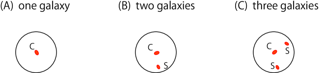
Figure 1: Case analysis of galaxy distribution in halos. (A) Case where one galaxy in a halo is a central galaxy in one halo. (B) Case where two galaxies in a halo are a pair of a central galaxy and a satellite galaxy in one halo. (C) Case where three galaxies in a halo are a combination of a central galaxy and two satellite galaxies in one halo.

II.2 Halo approach

The halo approach is useful to describe distributions of dark matter as well as distributions of galaxies from large to small scales White ; Seljak ; Scoccimarro2001 ; CooraySheth2002 . In this approach, all dark matter and galaxies are associated with virialized dark matter halos. The basic quantities of this approach are the dark matter density profile of a halo $\rho(r)$ and the halo mass function $dn/dM$.

In the present paper, we assume the Navarro–Frenk–White (NFW) density profile NFWprofile ,

$$\rho(r)={\rho_{s}\over r/r_{s}(1+r/r_{s})^{2}},$$ (2.41)

where the characteristic density $\rho_{s}$ and characteristic scale $r_{s}$ are fitting parameters. The virial mass of a halo within the virial radius $r_{\rm vir}$, which is related to the concentration parameter $c$ by $c=r_{\rm vir}/r_{s}$, is defined such that the averaged density within the radius is $\Delta_{\rm vir}$ times of the mean matter density $\bar{\rho}_{m}(z)$. Then, the virial mass $M_{\rm vir}$ is written as

$$M_{\rm vir}=4\pi\int_{0}^{r_{\rm vir}}drr^{2}\rho(r)=4\pi\rho_{s}r_{s}^{3}\left(\ln(1+r/r_{s})-{r/r_{s}\over 1+r/r_{s}}\right)={4\pi\over 3}r_{\rm vir}^{3}\Delta_{\rm vir}(z)\bar{\rho}_{m}(z),$$ (2.42)

where we adopt $\Delta_{\rm vir}=265$ at $z=0.3$. We use $M_{\rm vir}$ as the mass of halos. Then, we introduce the Fourier transform of the truncated NFW profile (see Scoccimarro2001 ; CooraySheth2002 ),

$$\tilde{u}_{\rm NFW}(k;M) = {\int_{r\leq r_{\rm vir}}d^{3}x\rho(r)e^{-i{\bm{k}}\cdot{\bm{x}}}\over\int_{r\leq r_{\rm vir}}d^{3}x\rho(r)}$$

$$= {4\pi\rho_{s}r_{s}^{3}\over M}\biggl{\{}\sin(kr_{s})\left[Si([1+c]kr_{s})-Si(kr_{s})\right]\ -{\sin ckr_{s}\over(1+c)kr_{s}}+\cos(kr_{s})\left[Ci([1+c]kr_{s})-Ci(kr_{s})\right]\biggr{\}},$$

where $C_{i}(x)$ and $S_{i}(x)$ are defined by

$$C_{i}(x)=-\int_{x}^{\infty}{\cos t\over t}dt,~{}~{}~{}~{}~{}~{}S_{i}(x)=\int_{0}^{x}{\sin t\over t}dt.~{}~{}~{}~{}~{}~{}$$ (2.44)

Because we are interested in the distribution of galaxies, we introduce the halo occupation distribution $N_{\rm HOD}(M)$, which describes the average number of galaxies inside a halo with mass $M$. In our approach, we introduce a description with central and satellite galaxies. Central galaxies reside at the centers of halos, while satellite galaxies reside in off-center regions of halos with large random velocities. We use the following form of the HOD with central galaxies and satellite galaxies Zheng2005 ,

$$N_{\rm HOD}(M)=\langle N_{\rm cen}\rangle(1+\langle N_{\rm sat}\rangle),$$ (2.45)

$$\langle N_{\rm cen}\rangle=\frac{1}{2}\left[1+{\rm erf}\left(\frac{\log_{10}(M)-\log_{10}(M_{\rm min})}{\sigma_{\log M}}\right)\right],$$ (2.46)

$$\langle N_{\rm sat}\rangle=\left(\frac{M-M_{\rm cut}}{M_{1}}\right)^{\alpha},$$ (2.47)

where ${\rm erf}(x)$ is the error function. We adopt the HOD parameters listed in Table I for the SDSS LRG catalog ReidSpergel and for the SDSS-III BOSS LOWZ catalog Parejko . Assuming that the number of groups with $N_{\rm sat}$ satellites follows the Poisson distribution Kravtsov2004 , the averaged satellite–satellite pair number $\langle N_{\rm sat}(N_{\rm sat}-1)\rangle$ per halo goes to $\langle N_{\rm cen}\rangle\langle N_{\rm sat}\rangle^{2}$. A deviation from the Poisson distribution for smaller halos could be influential for estimating the second and third moments of the galaxy distribution within a halo. We have checked the effect by introducing the formulas $\langle N_{\rm sat}(N_{\rm sat}-1)\rangle=\alpha^{2}(M)\langle N_{\rm sat}\rangle^{2}$ and $\langle N_{\rm sat}(N_{\rm sat}-1)(N_{\rm sat}-2)\rangle=\alpha^{3}(M)\langle N_{\rm sat}\rangle^{3}$ with $\alpha(M)$ defined in Refs. Scranton2002 ; TakadaJain ; Scoccimarro2001a

$$\alpha(M)=\left\{\begin{array}[]{ll}1&~{}{\rm for}~{}M\geq 10^{13}h^{-1}M_{\odot},\\ \ln\sqrt{M/10^{11}h^{-1}M_{\odot}}&~{}{\rm for}~{}M<10^{13}h^{-1}M_{\odot}.\\ \end{array}\right.$$ (2.50)

However, this effect does not alter our results because the halo mass of the galaxy samples adopted in the present work is large.

	LRG	LOWZ
$M_{\rm min}$	$5.7\times 10^{13}h^{-1}M_{\odot}$	$1.5\times 10^{13}h^{-1}M_{\odot}$
$\sigma_{\log M}$	0.7	0.45
$M_{\rm cut}$	$3.5\times 10^{13}h^{-1}M_{\odot}$	$1.4\times 10^{13}h^{-1}M_{\odot}$
$M_{1}$	$3.5\times 10^{14}h^{-1}M_{\odot}$	$1.3\times 10^{14}h^{-1}M_{\odot}$
$\alpha$	$1$	$1.38$

Table 1: HOD parameters for the LRG samples ReidSpergel and the LOWZ sample Parejko .

We assume that the distribution of satellite galaxies follows the NFW profile, and that the Fourier transform of the truncated NFW profile (LABEL:tuNFW) represents the power spectrum of the one-halo term. These assumptions do not alter our results. We assume that the satellite galaxies have internal random velocities following a Gaussian distribution specified by the one-dimensional velocity dispersion HikageYamamoto ; Kanemaru ; ReidSpergel ; LokasMamon ,

$$\sigma_{v,{\rm off}}(M)=\left({GM\over 2r_{\rm vir}}\right)^{1/2}.$$ (2.51)

These random motions cause the Fingers of God (FoG) effect, which changes the distribution of satellite galaxies in redshift space. Assuming that satellite motions in a halo are uncorrelated with each other, then the Fourier transform of the distribution of the satellite galaxies in redshift space is obtained (e.g., HikageYamamoto ) as

$$\widetilde{u}(\bm{k},M) = \tilde{u}_{\rm NFW}(k;M)\exp\left[-\frac{\sigma_{v,{\rm off}}^{2}(M)k^{2}\mu^{2}}{2a^{2}H^{2}(z)}\right].$$ (2.52)

The other key quantity of the halo-approach description is the halo mass function $dn/dM$, which is the number density of halos with mass $M$ per unit volume and per unit mass. For the halo mass function, we adopt the fitting formula in Refs. ShethTormen1999 ; ShethTormen2002 ; Parkinson2007

$$M{dn\over dM}={\bar{\rho}_{m}\over M}{d\ln\sigma_{R}^{-1}\over d\ln M}f(\sigma_{R})$$ (2.53)

with

$$f(\sigma_{R})=0.322\sqrt{2\times 0.707\over\pi}\left[1+\left({1\over 0.707\nu^{2}}\right)^{0.3}\right]{\nu}\exp\left(-{0.707\nu^{2}\over 2}\right),$$ (2.54)

and $\nu=\delta_{c}/\sigma(R)$, where $\sigma_{R}$ is the root mean square fluctuation in spheres containing mass $M$ at the initial time, which is extrapolated to the redshift $z$ using linear theory, $\delta_{c}$ is the critical value of the initial overdensity which is required for collapse, and $\delta_{c}=1.686$ is adopted.

For the linear bias $b(M)$, we adopt the halo bias of the fitting function,

$$b(M)=1-{\nu^{a}\over\nu^{a}+\delta_{c}^{a}}+0.183\nu^{b}+0.265\nu^{c}$$ (2.55)

with $a=0.132$, $b=1.5$ and $c=2.4$, which was calibrated using N-body simulations Tinker .

The power spectrum in the halo approach is given by a combination of the one-halo term and the two-halo term (see HikageYamamoto ),

$$P_{g}(t,\bm{k})=P_{g,1h}(t,{\bm{k}})+P_{g,2h}(t,{\bm{k}}).$$ (2.56)

The one-halo term is given by

$$P_{g,1h}(t,{\bm{k}})={1\over{\bar{n}}^{2}}\int dM{dn\over dM}\left[2\left<N_{c}\right>\left<N_{s}\right>\widetilde{u}({\bm{k}},M)+\left<N_{s}(N_{s}-1)\right>\widetilde{u}^{2}({\bm{k}},M)\right],$$ (2.57)

where $\bar{n}$ is the mean number density of galaxies given by

$$\bar{n}=\int dM{dn\over dM}N_{\rm HOD}(M),$$ (2.58)

while the two-halo term is given by

$$P_{g,2h}(t,{\bm{k}})={1\over{\bar{n}}^{2}}\prod_{i=1}^{2}\left[\int dM_{i}{dn\over dM_{i}}\left<N_{c}\right>\left\{1+\left<N_{s}\right>\widetilde{u}({\bm{k}},M)\right\}(b(M_{i})+f\mu^{2})\right]P_{m}(t,k),$$ (2.59)

where $P_{m}(t,k)$ is the matter power spectrum at the time $t$, for which we use the nonlinear fitting formula for the matter power spectrum NFWprofile . We also use the fitting formula of the linear growth rate $f={d\log D_{1}(a)/d\log a}=[\Omega_{m}(a)]^{\gamma}$, where $\Omega_{m}(a)$ is the matter density parameter at the scale factor $a=a(t)$ and $\gamma=0.55$.

The one-halo term of the power spectrum (2.57) represents the contribution from a pair of galaxies in one halo, as is shown in panel (B) of Fig. 1. The two-halo term (2.59) represents the contribution from a pair of galaxies in two different halos, as are obtained by combinations of the galaxies in each panel of Fig. 1.

In Ref. HikageYamamoto , using the SDSS LRG sample, the authors demonstrated that satellite galaxies make a significant contribution to the multipole power spectrum even when their fraction is small, where the multipole galaxy power spectrum of $P_{g}(t,\bm{k})$ is defined by

$$P^{\ell}(t,k)=\int_{-1}^{+1}d\mu P_{g}(t,{\bm{k}}){\cal L}_{\ell}(\mu),$$ (2.60)

using the Legendre polynomial ${\cal L}_{\ell}(\mu)$ with $\mu=\bm{\gamma}\cdot\bm{k}/k$. The one-halo term, describing the FoG effect of satellite galaxies, makes the dominant contribution to the higher multipole spectra with $\ell\geq 2$. It is also demonstrated that small-scale information of the higher multipole spectrum is useful for calibrating the satellite FoG effect and testing gravity theory on halo scales Kanemaru and dramatically improves the measurement of the cosmic growth rate Hikage .

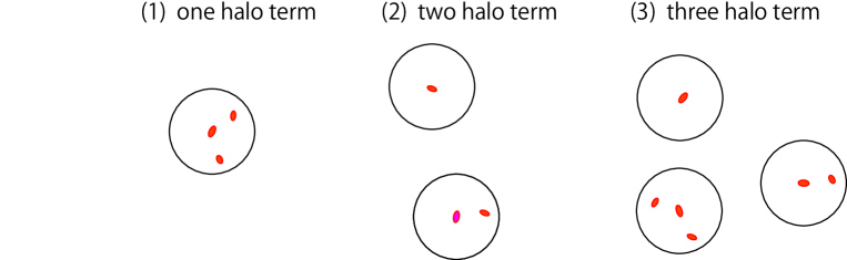
Figure 2: Contributions of a (1) one-halo term, (2) two-halo term, and (3) three-halo term to the bispectrum. (1) A one-halo term represents the contribution from three galaxies in one halo. (2) A two-halo term represents the contribution from the combination of two halos with one galaxy and two galaxies in each halo. (3) A three-halo term represents the contribution from three halos with each galaxy.

III Bispectrum in the halo approach

Figure 3: Definition of variables for the bispectrum (see also Table II).

Variables	Meaning
$k_{i}$	Magnitude of the wavenumber vector $\bm{k}_{i}$
$\hat{\bm{k}}_{i}$	Unit vector of the wavenumber vector $\bm{k}_{i}$
$\mu_{i}(=\hat{\bm{k}}_{i}\cdot\bm{\gamma})$	Cosine of the angle between $\bm{k}_{i}$ and the line of sight direction $\bm{\gamma}$
$\mu(=\mu_{1})$	Cosine of the angle ($\omega$) between $\bm{k}_{1}$ and the line of sight direction $\bm{\gamma}$
$\theta_{12}(=\theta)$	Angle between $\bm{k}_{1}$ and $\bm{k}_{2}$
$\omega$	Angle between $\bm{k}_{1}$ and the line of sight direction $\bm{\gamma}$
$\phi$	Azimuthal angle of the line of sight direction $\bm{\gamma}$ around $\bm{k}_{1}$

Table 2: Definition of the variables for the bispectrum (see also Figure 3). The bispectrum is the function of the five variables, $k_{1}$, $k_{2}$, $\theta$, $\omega$, and $\phi$.

III.1 Variables for the bispectrum in redshift space

The bispectrum with the halo approach is investigated in Ref. smith2008 . In the present paper, as a generalization of a previous work smith2008 , we present an analytic expression for the bispectrum applying the halo approach with the HOD description with central galaxies and satellite galaxies. We focus on the bispectrum $B_{g}(t,\bm{k}_{1},\bm{k}_{2},\bm{k}_{3})$, which is defined by

$$\left\langle\delta(t,\bm{k}_{1})\delta(t,\bm{k}_{3})\delta(t,\bm{k}_{3})\right\rangle=(2\pi)^{3}\delta_{D}^{(3)}(\bm{k}_{1}+\bm{k}_{2}+\bm{k}_{3})B_{g}(t,\bm{k}_{1},\bm{k}_{2},\bm{k}_{3}).$$ (3.61)

Thus the bispectrum $B_{g}(t,\bm{k}_{1},\bm{k}_{2},\bm{k}_{3})$ implicitly assumes ${\bm{k}}_{1}+{\bm{k}}_{2}+{\bm{k}}_{3}=0$. Since we have the constraint ${\bm{k}}_{1}+{\bm{k}}_{2}+{\bm{k}}_{3}=0$, the bispectrum is described by the five parameters, $k_{1}$, $k_{2}$, $\cos\theta_{12}(={{\bm{k}}}_{1}\cdot{\bm{k}}_{2}/k_{1}k_{2})$, $\mu(=\cos\omega)$, and $\phi$, as variables of the bispectrum, with which we write the vectors

$${\bm{k}}_{1}=(0,0,k_{1}),$$ (3.62)

$${\bm{k}}_{2}=(0,k_{2}\sin\theta_{12},k_{2}\cos\theta_{12}),$$ (3.63)

$${\bm{k}}_{3}=(0,-k_{2}\sin\theta_{12},-k_{1}-k_{2}\cos\theta_{12}),$$ (3.64)

$${\bm{\gamma}}=(\sin\omega\cos\phi,\sin\omega\sin\phi,\cos\omega).$$ (3.65)

For the configuration of the variables, see Fig. 3 and Table II. Then, we can write $\mu_{i}$ as

$$\mu_{1}={\hat{\bm{k}}}_{1}\cdot{\bm{\gamma}}=\cos\omega=\mu,$$ (3.66)

$$\mu_{2}={\hat{\bm{k}}}_{2}\cdot{\bm{\gamma}}=\sin\theta_{12}\sin\omega\sin\phi+\cos\theta_{12}\cos\omega=\sin\theta_{12}\sqrt{1-\mu^{2}}\sin\phi+\cos\theta_{12}\mu,$$ (3.67)

$$\mu_{3}=-{k_{1}\over k_{3}}\mu_{1}-{k_{2}\over k_{3}}\mu_{2},$$ (3.68)

with ${k}_{3}^{2}=(k_{2}\sin\theta_{12})^{2}+(k_{1}+k_{2}\cos\theta_{12})^{2}$. Hereafter, we use the notation $\theta=\theta_{12}$.

III.2 Expression for the bispectrum in redshift space

The bispectrum in the halo approach consists of the one-halo term $B_{g,1h}$, the two-halo term $B_{g,2h}$, and the three-halo term $B_{g,3h}$ as

$$B_{g}(t,\bm{k}_{1},\bm{k}_{2},\bm{k}_{3})=B_{g,1h}(t,{\bm{k}}_{1},{\bm{k}}_{2},{\bm{k}}_{3})+B_{g,2h}(t,{\bm{k}}_{1},{\bm{k}}_{2},{\bm{k}}_{3})+B_{g,3h}(t,{\bm{k}}_{1},{\bm{k}}_{2},{\bm{k}}_{3}),$$ (3.69)

which are written as

$$B_{g,1h}(t,{\bm{k}}_{1},{\bm{k}}_{2},{\bm{k}}_{3}) = {1\over\bar{n}^{3}}\int dM{dn(M)\over dM}\biggl{[}\left<N_{c}\right>\left<N_{s}(N_{s}-1)\right>\left(\widetilde{u}({\bm{k}}_{1},M)\widetilde{u}({\bm{k}}_{2},M)+2~{}{\rm cyclic~{}terms}\right)$$ (3.70)

$$+\left<N_{s}(N_{s}-1)(N_{s}-2)\right>\widetilde{u}({\bm{k}}_{1},M)\widetilde{u}({\bm{k}}_{2},M)\widetilde{u}({\bm{k}}_{3},M)\biggr{]},$$

$$B_{g,2h}(t,{\bm{k}}_{1},{\bm{k}}_{2},{\bm{k}}_{3}) = {1\over\bar{n}^{3}}\int dM_{1}{dn(M_{1})\over dM_{1}}\biggl{[}\left<N_{c}\right>\left<N_{s}\right>\left(\widetilde{u}({\bm{k}}_{1},M_{1})+\widetilde{u}({\bm{k}}_{2},M_{1})\right)+\left<N_{s}(N_{s}-1)\right>\widetilde{u}({\bm{k}}_{1},M_{1})\widetilde{u}({\bm{k}}_{2},M_{1})\biggr{]}$$ (3.71)

$$\times\int dM_{2}{dn(M_{2})\over dM_{2}}\left(\left<N_{c}\right>+\left<N_{c}\right>\left<N_{s}\right>\widetilde{u}({\bm{k}}_{3},M_{2})\right)P_{2h}(t,{\bm{k}}_{3},M_{1},M_{2})+2~{}{\rm cyclic~{}terms},$$

$$B_{g,3h}(t,{\bm{k}}_{1},{\bm{k}}_{2},{\bm{k}}_{3}) = {1\over\bar{n}^{3}}\int\prod_{i=1}^{3}\left[dM_{i}{dn(M_{i})\over dM_{i}}\left<N_{c}\right>\left(1+\left<N_{s}\right>\widetilde{u}({\bm{k}}_{i},M_{i})\right)\right]P_{3h}(t,{\bm{k}}_{1},{\bm{k}}_{2},{\bm{k}}_{3},M_{1},M_{2},M_{3}),$$ (3.72)

where we define

$$P_{2h}(t,{\bm{k}}_{3},M_{1},M_{2})=(b(M_{1})+\mu_{3}^{2}f)(b(M_{2})+\mu_{3}^{2}f)P_{m}^{\rm NL}(t,k_{3}),$$ (3.73)

$$P_{3h}(t,{\bm{k}}_{1},{\bm{k}}_{2},{\bm{k}}_{3},M_{1},M_{2},M_{3})=2P_{m}(t,k_{1})P_{m}(t,k_{2})Z_{1}({\bm{k}}_{1},M_{1})Z_{1}({\bm{k}}_{2},M_{2})Z_{2}({\bm{k}}_{1},{\bm{k}}_{2},M_{3})+2~{}{\rm cyclic~{}terms}$$ (3.74)

with

$$Z_{1}({\bm{k}}_{1},M_{1})=b(M_{1})+f\mu_{1}^{2},$$ (3.75)

$$Z_{1}({\bm{k}}_{2},M_{2})=b(M_{2})+f\mu_{2}^{2},$$ (3.76)

$$Z_{2}({\bm{k}}_{1},{\bm{k}}_{2},M_{3})=b(M_{3})F_{2}({\bm{k}}_{1},{\bm{k}}_{2})+{b_{2}(M_{3})\over 2}+f\mu_{12}^{2}G_{2}({\bm{k}}_{1},{\bm{k}}_{2})$$

$$~{}~{}~{}~{}~{}~{}~{}~{}~{}~{}~{}~{}~{}+{1\over 2}f\mu_{12}k_{12}\left\{{\mu_{1}\over k_{1}}\left(b(M_{3})+f\mu_{2}^{2}\right)+{\mu_{2}\over k_{2}}\left(b(M_{3})+f\mu_{1}^{2}\right)\right\},$$ (3.77)

$\mu_{12}=({\bm{k}}_{1}+{\bm{k}}_{2})\cdot{\bm{\gamma}}/k_{12}$, and $k_{12}=|{\bm{k}}_{1}+{\bm{k}}_{2}|$. The directional cosine between the vector ${\bm{k}}_{j}$ and the line-of-sight direction is $\mu_{j}={\bm{k}}_{j}\cdot{{\bm{\gamma}}}/k_{j}$. Hereafter, we set $b_{2}=0$ unless otherwise stated explicitly.

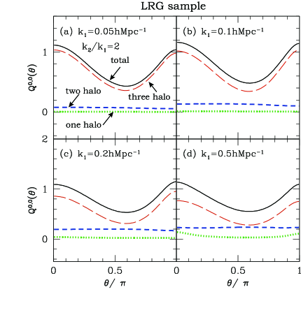
Figure 4: Left figure shows $Q^{0,0}(\theta)$ with the LRG sample by fixing (a) $k_{1}=0.05$, (b) $k_{1}=0.1$, (c) $k_{1}=0.2$, and (d) $k_{1}=0.5$ in the unit $h$/Mpc, and $k_{2}/k_{1}=2$. In each panel the (green) dotted curve is the one-halo term contribution, the (blue) short-dashed curve is the two-halo term contribution, the (red) long-dashed curve is the three-halo term contribution, and the (black) solid curve is the total combination. The right figure shows the same as the left figure but for the LOWZ sample.

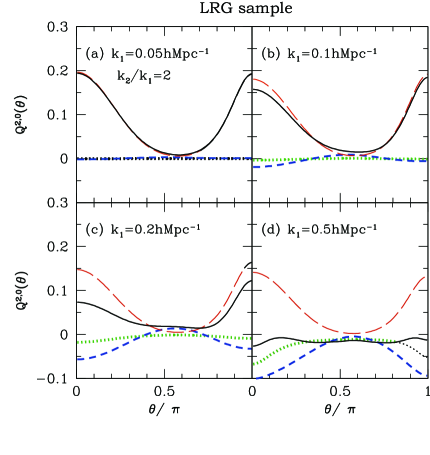
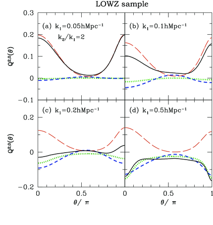
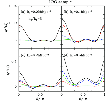
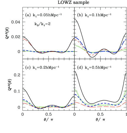
Figure 5: Same as Fig. 4, but for $Q^{2,0}(\theta)$.

Figure 6: Same as Fig. 4, but for $Q^{4,0}(\theta)$.

We introduce the multipole of the bispectrum scoccimarro1999 ; scoccimarro2015 ,

$$B^{\ell,0}(k_{1},k_{2},{\theta}) = {1\over 4\pi}\int_{0}^{2\pi}d\phi\int_{-1}^{+1}d\cos\omega B_{g}(t,k_{1},k_{2},{\theta},\omega,\phi){\cal L}_{\ell}(\cos\omega),$$ (3.78)

where ${\cal L}_{\ell}(\mu)$ is the Legendre polynomial. Then, we define the multipoles of the reduced bispectrum as

$$Q^{\ell,0}(k_{1},k_{2},{\theta})={B^{\ell,0}(k_{1},k_{2},{\theta})\over P^{0}(t,k_{1})P^{0}(t,k_{2})+P^{0}(t,k_{2})P^{0}(t,k_{3})+P^{0}(t,k_{3})P^{0}(t,k_{1})},$$ (3.79)

where $P^{0}(t,k_{i})$ is the monopole spectrum of the galaxy power spectrum $P_{g}(t,\bm{k}_{i})$, which is defined by Eq. (2.56). Because $B_{g}(t,k_{1},k_{2},\theta,\omega,\phi)$ consists of the one-halo term, the two-halo term, and the three-halo term, $B^{\ell,0}(k_{1},k_{2},\theta)$ and $Q^{\ell,0}(k_{1},k_{2},{\theta})$ are written as the sum of the corresponding three components,

$$B^{\ell,0}(k_{1},k_{2},\theta)=B_{1h}^{\ell,0}(k_{1},k_{2},\theta)+B_{2h}^{\ell,0}(k_{1},k_{2},\theta)+B_{3h}^{\ell,0}(k_{1},k_{2},\theta)$$ (3.80)

and

$$Q^{\ell,0}(k_{1},k_{2},\theta)=Q_{1h}^{\ell,0}(k_{1},k_{2},\theta)+Q_{2h}^{\ell,0}(k_{1},k_{2},\theta)+Q_{3h}^{\ell,0}(k_{1},k_{2},\theta).$$ (3.81)

III.3 Behaviors of the multipoles of the bispectrum

III.3.1 Monopole of the bispectrum $Q^{0,0}(k_{1},k_{2},{\theta})$

Figure 4 shows the monopole $Q^{0,0}(k_{1},k_{2},{\theta})$ as a function of $\theta(=\theta_{12})$, where $k_{1}$ and $k_{2}(=2k_{1})$ are fixed as shown in each panel. Here the left panels adopt the HOD parameters of the SDSS-II LRG sample, while the right panels adopt those of the SDSS-III BOSS LOWZ sample. $Q^{0,0}_{1h}(k_{1},k_{2},\theta)$ does not make a significant contribution to $Q^{0,0}(k_{1},k_{2},\theta)$ at scales of $k<0.1~{}h$/Mpc, but it makes non-negligible contribution at scales of $k>0.1~{}h$/Mpc. $Q^{0,0}_{2h}(k_{1},k_{2},\theta)$ makes significant contribution to $Q^{0,0}(k_{1},k_{2},\theta)$, which is almost constant as a function of $\theta$ for $k<0.5~{}h$/Mpc.

III.3.2 Higher multipoles of the bispectrum $Q^{2,0}(k_{1},k_{2},{\theta})$ and $Q^{4,0}(k_{1},k_{2},{\theta})$

Figures 6 and 6 show the same as Fig. 4 but for $Q^{2,0}(k_{1},k_{2},{\theta})$ and $Q^{4,0}(k_{1},k_{2},{\theta})$, respectively. One can recognize the following features from these figures: For the higher multipoles $Q^{\ell,0}(k_{1},k_{2},\theta)$ with $\ell=2$ and $4$, the one-halo term and the two-halo term make a significant contribution for $k\lower 2.15277pt\hbox{$\;\buildrel>\over{\sim}\;$}0.1~{}h$/Mpc. The contribution from the one-halo term and the two-halo term to the multipole bispectrum is more significant in the LOWZ sample than that in the LRG sample.

Figure 7: Comparison of $Q^{\ell,0}(\theta)$ between our theoretical model and numerical simulations adopting the HOD of the LOWZ sample. The top panels, the middle panels, and the bottom panels show $Q^{0,0}$, $Q^{2,0}$ and $Q^{4,0}$ as functions of $\theta$. The wave number $k_{1}/[h{\rm Mpc}^{-1}]$ is fixed as $0.05$, $0.1$, $0.2$ and $0.3$, from left to right, while the ratio of $k_{1}$ to $k_{2}$ is fixed equally as $k_{2}/k_{1}=2$. In each panel, the solid curve is our theoretical model, while the dash–dotted curve is the same except for setting $\sigma_{v,{\rm off}}=0$. The meaning of $\sigma_{v,{\rm off}}=0$ is that the random velocity of the satellite galaxy is neglected, thus the FoG effect is neglected. The data with error bars are the results from mock catalogs from numerical simulations. The thick (green) data points and thin (red) data points respectively correspond to the cases in the presence and absence of $\sigma_{v,{\rm off}}$, corresponding to the solid curve and the dash–dotted curve. All values in the bottom left two panels are multiplied by a factor of $5$.

III.3.3 Comparison with the results of mock catalogs

For comparison with our analytic model, we construct simulated samples assuming the HOD of the SDSS-III BOSS LOWZ sample. We run 10 realizations of N-body simulations at the side length of $1h^{-1}$Gpc with the number of mass particles set as 800³ (mass for each particle set as $1.3\times 10^{11}h^{-1}M_{\odot}$) using Gadget-2 code (Springel05, ). The softening length is set to be $50h^{-1}$kpc. The initial mass distribution is Gaussian starting from $z=49$ generated by the 2LPT code of (Crocce06, ). We adopt a flat $\Lambda$CDM cosmology with the following parameters: $\Omega_{b}=0.046$, $\Omega_{m}=0.273$, $n_{s}=0.963$, $h=0.704$, $\tau=0.089$, and $\sigma_{8}=0.809$. The halo is identified with the friends-of-friends algorithm with a linking length of 0.2. The minimum number of mass particles is 10, corresponding to the mass of $1.3\times 10^{12}h^{-1}M_{\odot}$. When comparing with our theoretical model, we add this cut of minimum mass in the integration of mass. The central and satellite galaxies are assigned to each halo to follow the HOD of BOSS LOWZ sample. The position and velocity of each central galaxy are given as the arithmetic mean of all particles in the halo. The position and velocity of satellites are defined as those of randomly-selected mass particles. We confirmed that the mass resolution of our simulation is sufficient for the following comparison with our theoretical model. The data points with error bars in each panel of Fig. 7 are the results of the numerical simulations. The error bars represent 1-sigma dispersion of $10$ simulation results divided by $\sqrt{10}$, which roughly corresponds to the sample variance for $10({\rm Gpc}/h)^{3}$ volume data. The binning widths of $k_{1},k_{2}$ and $\theta$ are set to be $0.01h/$Mpc, $0.02h/$Mpc and $\pi/12$, respectively.

Figure 7 shows a comparison between our analytic model of the multipoles of the reduced bispectrum and results of numerical simulations at various wave numbers of $k_{1}(=k_{2}/2)$ (see the caption of Fig. 7). Here we adopt the HOD of the SDSS-III BOSS LOWZ sample. In each panel of this figure, the solid curve is the analytic model, while the data points with the thick (green) error bars are from the numerical simulations. The dash-dotted curve is the analytic model prediction but with settings such that the random velocity of the satellite galaxies is zero, i.e., $\sigma_{v,{\rm off}}=0$. The data points with the thin (red) error bars are the results of the numerical simulation assuming that satellite galaxies have the same velocities as those of the central galaxy in the halos, corresponding to the theoretical curve with setting $\sigma_{v,{\rm off}}=0$. Figure 7 shows that our theoretical model well explains the characteristic behavior of the bispectrum from the numerical simulations, though some differences arise for the cases with larger wavenumbers at a quantitative level. However, the behaviors of the simulations are reproduced at a qualitative level.

IV Approximate formula

We have found that the characteristic behaviors of the multipoles of the bispectrum can be explained by our analytic model. Further, we derive analytic approximate formulas for the multipoles of the bispectrum, which will be useful to understand the physical properties and the origin of the characteristic behaviors of the multipoles of the bispectrum.

According to the case of the multipole power spectrum HikageYamamoto , we assume the following approximate formulas for the one-halo term, the two-halo term, and the three-halo term,

$$B_{g,1h}(t,{\bm{k}}_{1},{\bm{k}}_{2},{\bm{k}}_{3}) \simeq {f_{s}^{2}\over\bar{n}^{2}}\left(\widetilde{u}({\bm{k}}_{1})\widetilde{u}({\bm{k}}_{2})+\widetilde{u}({\bm{k}}_{2})\widetilde{u}({\bm{k}}_{3})+\widetilde{u}({\bm{k}}_{3})\widetilde{u}({\bm{k}}_{1})\right),$$ (4.82)

$$B_{g,2h}(t,{\bm{k}}_{1},{\bm{k}}_{2},{\bm{k}}_{3}) \simeq {f_{s}\over\bar{n}}\left(\widetilde{u}({\bm{k}}_{1})+\widetilde{u}({\bm{k}}_{2})\right)(\bar{b}+\mu_{3}^{2}f)^{2}P_{m}(k_{3})+2~{}{\rm cyclic~{}terms},$$ (4.83)

$$B_{g,3h}(t,{\bm{k}}_{1},{\bm{k}}_{2},{\bm{k}}_{3}) \simeq 2P_{m}(t,k_{1})P_{m}(t,k_{2})(\bar{b}+\mu_{1}^{2}f)(\bar{b}+\mu_{2}^{2}f)\Bigl{[}\bar{b}F_{2}({\bm{k}}_{1},{\bm{k}}_{2})+f\mu_{3}^{2}G_{2}({\bm{k}}_{1},{\bm{k}}_{2})+{\bar{b}_{2}\over 2}$$ (4.84)

$$-{1\over 2}f\mu_{3}k_{3}\Bigl{(}{\mu_{1}\over k_{1}}(\bar{b}+f\mu_{2}^{2})+{\mu_{2}\over k_{2}}(\bar{b}+f\mu_{1}^{2})\Bigr{)}\Bigr{]}+2~{}{\rm cyclic~{}terms},$$

where we use the approximate formula

$$\widetilde{u}({\bm{k}_{i}})\simeq\exp\left[-\frac{\overline{\sigma}_{v,{\rm off}}^{2}k_{i}^{2}\mu^{2}}{2a^{2}H^{2}(z)}\right]=\exp\left[-{\lambda_{v,{\rm off}}^{2}k_{i}^{2}\mu^{2}}\right]$$ (4.85)

for $i=1,2$ and $3$, $\bar{b}$, and $\overline{\sigma}_{v,{\rm off}}$ are averaged values of the bias and the random velocity of satellite galaxies over the halo mass, and $f_{s}$ is the satellite fraction. Here we introduce the characteristic length scale, associated with the random motions by

$$\lambda_{v{\rm,off}}^{2}=\frac{\overline{\sigma}_{v,{\rm off}}^{2}}{2a^{2}H^{2}(z)},$$ (4.86)

and we include $\bar{b}_{2}$ as an averaged value of the bias parameter $b_{2}$.

IV.1 One-halo term

Following the definition of (3.78) and (3.80), by expanding the formulas by the power of $\lambda_{v,{\rm off}}^{2}$, we have the following approximate formulas for the contribution from the one-halo term

$$B_{1h}^{0,0}(k_{1},k_{2},\theta) \simeq {f_{s}^{2}\over\bar{n}^{2}}\left[3-{4\over 3}\left(k_{1}^{2}+k_{2}^{2}+k_{1}k_{2}\cos{\theta}\right){\lambda_{v,{\rm off}}^{2}}\right],$$ (4.87)

$$B_{1h}^{2,0}(k_{1},k_{2},\theta) \simeq -{2\over 15}{f_{s}^{2}\over\bar{n}^{2}}\left(4k_{1}^{2}+k_{2}^{2}(1+3\cos 2{\theta})+4k_{1}k_{2}\cos{\theta}\right){\lambda_{v,{\rm off}}^{2}},$$ (4.88)

$$B_{1h}^{4,0}(k_{1},k_{2},\theta) = {\cal O}\left({f_{s}^{2}\over\bar{n}^{2}}\left({k^{2}\lambda_{v,{\rm off}}^{2}}\right)^{2}\right).$$ (4.89)

Thus, the contribution from the one-halo term to the multipole bispectrum is on the order of $f_{s}^{2}/\bar{n}^{2}$. The dominant term in the monopole $B_{1h}^{0,0}$ is constant $3f_{s}^{2}/\bar{n}^{2}$ for $k^{2}\lambda_{v,{\rm off}}^{2}\ll 1$ from (4.87), however, $k$ and $\theta$ dependence arises for $k^{2}\lambda_{v,{\rm off}}^{2}\lower 2.15277pt\hbox{$\;\buildrel>\over{\sim}\;$}1$. The order of higher multiple bispectrum $B^{\ell,0}_{{1h}}$ is roughly ${\cal O}((f_{s}^{2}/\bar{n}^{2})(k\lambda_{v,{\rm off}})^{\ell})$ for $\ell=2$ and $4$.

Thus, one can roughly write the approximate formulas for term contribution to the multiple bispectrum as

$$B_{1h}^{0,0}(k_{1},k_{2},\theta)\sim\left({f_{s}\over\bar{n}}\right)^{2}\left(3-{\cal O}(k^{2}\lambda_{v,{\rm off}}^{2})\right),$$ (4.90)

$$B_{1h}^{2,0}(k_{1},k_{2},\theta)\sim\left({f_{s}\over\bar{n}}\right)^{2}{\cal O}\left(k^{2}\lambda_{v,{\rm off}}^{2}\right),$$ (4.91)

$$B_{1h}^{4,0}(k_{1},k_{2},\theta)\sim\left({f_{s}\over\bar{n}}\right)^{2}{\cal O}\left(k^{4}\lambda_{v,{\rm off}}^{4}\right).$$ (4.92)

IV.2 Two-halo term

Similarly, one can derive the contribution from the two halo term to the monopole bispectrum and the quadrupole bispectrum as

$$B_{2h}^{0,0}(k_{1},k_{2},\theta)\simeq{f_{s}\over\bar{n}}\Bigl{[}\Bigl{(}2\bar{b}^{2}+{4bf\over 3}+{2f^{2}\over 5}\Bigr{)}(P_{m}(k_{1})+P_{m}(k_{2})+P_{m}(k_{3}))$$

$$~{}~{}~{}~{}+{\lambda_{v,{\rm off}}^{2}\over 105}\Bigl{\{}{P_{m}(k_{1})}\Bigl{(}-(35b^{2}+42bf+15f^{2})k_{1}^{2}-2(35\bar{b}^{2}+28\bar{b}f+9f^{2})k_{2}^{2}-2(35\bar{b}^{2}+42\bar{b}f+15f^{2})k_{1}k_{2}\cos{\theta}$$

$$~{}~{}~{}~{}-4f(7\bar{b}+3f)k_{2}^{2}\cos 2{\theta}\Bigr{)}+{P_{m}(k_{2})}\Bigl{(}-2(35\bar{b}^{2}+28\bar{b}f+9f^{2})k_{1}^{2}-(35\bar{b}^{2}+42\bar{b}f+15f^{2})k_{2}^{2}-2(35\bar{b}^{2}+42\bar{b}f$$

$$~{}~{}~{}~{}+15f^{2})k_{1}k_{2}\cos{\theta}-4f(7\bar{b}+3f)k_{1}^{2}\cos 2{\theta}\Bigr{)}-{P_{m}(k_{3})\over k_{1}^{2}+k_{2}^{2}+2k_{1}k_{2}\cos{\theta}}\Bigl{(}35\bar{b}^{2}(k_{1}^{2}+k_{2}^{2})^{2}+14\bar{b}f(3k_{1}^{4}+4k_{1}^{2}k_{2}^{2}$$

$$~{}~{}~{}~{}+3k_{2}^{4})+3f^{2}(5k_{1}^{4}+6k_{1}^{2}k_{2}^{2}+5k_{2}^{4})+2k_{1}k_{2}\cos{\theta}(35\bar{b}^{2}+42\bar{b}f+15f^{2})(k_{1}^{2}+k_{2}^{2})+2f(7\bar{b}+3f)k_{1}k_{2}\cos 2{\theta}\Bigr{)}\Bigr{\}}\Bigr{]},$$

(4.93)

$$B_{2h}^{2,0}(k_{1},k_{2},\theta)\simeq{f_{s}\over 210\bar{n}}\Bigl{[}{16f(7\bar{b}+3f)}P_{m}(k_{1})+{4f(7\bar{b}+3f)}(1+3\cos 2{\theta})P_{m}(k_{2})$$

$$~{}~{}~{}~{}+{4f(7\bar{b}+3f)(4k_{1}^{2}+k_{2}^{2}+8k_{1}k_{2}\cos{\theta}+3k_{2}^{2}\cos 2{\theta})\over k_{1}^{2}+k_{2}^{2}+2k_{1}k_{2}\cos{\theta}}P_{m}(k_{3})+{\lambda_{v,{\rm off}}^{2}}\Bigl{\{}{2P_{m}(k_{1})}\Bigl{(}-2(\bar{b}+f)(7\bar{b}+5f)k_{1}^{2}$$

$$~{}~{}~{}~{}-(7\bar{b}^{2}+26\bar{b}f+11f^{2})k_{2}^{2}-4(\bar{b}+f)(7\bar{b}+5f)k_{1}k_{2}\cos{\theta}-(21\bar{b}^{2}+22\bar{b}f+9f)k_{2}^{2}\cos 2{\theta}\Bigr{)}$$

$$~{}~{}~{}~{}+{P_{m}(k_{2})}\Bigl{(}-2(28\bar{b}^{2}+26\bar{b}f+9f^{2})k_{1}^{2}-(\bar{b}+f)(7\bar{b}+5f)k_{2}^{2}-2(28\bar{b}^{2}+39\bar{b}f+15f^{2})k_{1}k_{2}\cos{\theta}$$

$$~{}~{}~{}~{}-(4f(11\bar{b}+5f)k_{1}^{2}+3(\bar{b}+f)(7\bar{b}+5f)k_{2}^{2})\cos 2{\theta}-2fk_{1}((9\bar{b}+5f)k_{2}\cos 3{\theta}+fk_{1}\cos 4{\theta})\Bigr{)}$$

$$~{}~{}~{}~{}-{P_{m}(k_{3})\over(k_{1}^{2}+k_{2}^{2}+2k_{1}k_{2}\cos{\theta})^{2}}\Bigl{(}4(\bar{b}+f)(7\bar{b}+5f)k_{1}^{6}+7(\bar{b}+f)(17\bar{b}+11f)k_{1}^{4}k_{2}^{2}+(77\bar{b}^{2}+142\bar{b}f$$

$$~{}~{}~{}~{}+63f^{2})k_{1}^{2}k_{2}^{4}+(\bar{b}+f)(7\bar{b}+5f)k_{2}^{6}+2k_{1}k_{2}\Bigl{\{}8(\bar{b}+f)(7\bar{b}+5f)k_{1}^{4}+(91\bar{b}^{2}+161\bar{b}f+66f^{2})k_{1}^{2}k_{2}^{2}$$

$$~{}~{}~{}~{}+(35\bar{b}^{2}+69\bar{b}f+30f^{2})k_{2}^{4}\Bigr{\}}\cos{\theta}+k_{2}^{2}\Bigl{\{}7(\bar{b}+f)(11\bar{b}+9f)k_{1}^{4}+2(49\bar{b}^{2}+88\bar{b}f+35f^{2})k_{1}^{2}k_{2}^{2}$$

$$~{}~{}~{}~{}+3(\bar{b}+f)(7\bar{b}+5f)k_{2}^{4}\Bigr{\}}\cos 2{\theta}+2k_{1}k_{2}^{3}\Bigl{\{}(21\bar{b}^{2}+31\bar{b}f+14f^{2})k_{1}^{2}+(21\bar{b}^{2}+27\bar{b}f+10f^{2})k_{2}^{2}\Bigr{\}}\cos 3{\theta}$$

$$~{}~{}~{}~{}+(21\bar{b}^{2}+18\bar{b}f+7f^{2})k_{1}^{2}k_{2}^{4}\cos 4{\theta}\Bigr{)}\Bigr{\}}\Bigr{]}.$$ (4.94)

Thus, the contribution of the two-halo term to the multipole bispectrum is in proportion to $f_{s}/\bar{n}$. The dominant term in the monopole bispectrum from the two-halo term is roughly on the order of $2(f_{s}/\bar{n})(P_{g}^{0}(k_{1})+P_{g}^{0}(k_{2})+P_{g}^{0}(k_{3}))$ for $k^{2}\lambda_{v,{\rm off}}^{2}\ll 1$, where $P_{g}^{0}(k)$ is the monopole galaxy power spectrum in linear theory, defined by

$$P_{g}^{\ell}(k)={1\over 2}\int_{-1}^{+1}d\mu\left(\bar{b}+f\mu^{2}\right)^{2}P_{m}(k){\cal L}_{\ell}(\mu)$$ (4.95)

with $\ell=0$. Explicitly, we write

$$P_{g}^{0}(k)=\left(\bar{b}^{2}+{2\bar{b}f\over 3}+{f^{2}\over 5}\right)P_{m}(k),$$ (4.96)

$$P_{g}^{2}(k)=\left({4\bar{b}f\over 15}+{4f^{2}\over 35}\right)P_{m}(k),$$ (4.97)

for $\ell=0$ and $2$. Similarly, the dominant terms of the quadrupole bispectrum $B_{2h}^{2,0}$ from the two-halo term contribution are $(f_{s}/\bar{n})P^{2}_{g}(k_{i})$ for $k^{2}\lambda_{v,{\rm off}}^{2}\ll 1$. However, other contributions depending on $k$ and $\theta$ significantly emerge for $k^{2}\lambda_{v,{\rm off}}^{2}\lower 2.15277pt\hbox{$\;\buildrel>\over{\sim}\;$}1$. These properties are common to $B_{2h}^{4,0}(k_{1},k_{2},\theta)$. For the higher multipoles, $B_{2h}^{\ell,0}(k_{1},k_{2},\theta)$ with $\ell\geq 2$, the contributions of the terms in proportion to $\lambda_{\rm off}^{2\ell}$ are important.

In summary, the two-halo term contribution to the multipole bispectrum is more important than that of the one-halo term, and can be roughly expressed as

$$B_{2h}^{\ell,0}(k_{1},k_{2},\theta)\sim\left({2f_{s}\over\bar{n}}\right)\left({\cal O}(P^{\ell}_{g}(k_{1})+P^{\ell}_{g}(k_{2})+P^{\ell}_{g}(k_{3}))-{\cal O}(P_{g}(k)k^{2}\lambda^{2}_{v,{\rm off}})\right)$$ (4.98)

for $\ell=0$ and $2$.

IV.3 Three-halo term

For an analytic description, we complete this section by presenting the analytic formula for the multipole bispectrum from the three-halo terms, which can be written as

$$B_{3h}^{\ell,0}(k_{1},k_{2},\theta)=C^{\ell}_{12}P_{m}(k_{1})P_{m}(k_{2})+C^{\ell}_{23}P_{m}(k_{2})P_{m}(k_{3})+C^{\ell}_{31}P_{m}(k_{3})P_{m}(k_{1}),$$ (4.99)

where $C^{\ell}_{12}$, $C^{\ell}_{23}$ and $C^{\ell}_{31}$ are listed in the Appendix.

The mathematical formulas of this section and those of the appendix are derived using Mathematica. The source Mathematica programs for the derivation are included in the source file uploaded at the site arXiv.org (Ref. YamamotoNanHikage ).

IV.4 Discussions

We find that $B_{1h}^{0,0}(k_{1},k_{2},\theta)$ and $B_{2h}^{0,0}(k_{1},k_{2},\theta)$ are symmetric with respect to the exchange of wavenumbers between $k_{1}$ and $k_{2}$. However, the higher multipoles $B_{1h}^{\ell,0}(k_{1},k_{2},\theta)$ and $B_{2h}^{\ell,0}(k_{1},k_{2},\theta)$ with $\ell\geq 2$ do not show the symmetric property.

In the above expressions, (4.87) and (4.93), the contribution to the monopole bispectrum from the one-halo term and from the two-halo term, respectively, the dominant terms in the limit $k^{2}\lambda_{v,{\rm off}}^{2}\ll 1$ are positive and almost constant as functions of $\theta$. On the other hand, for $k^{2}\lambda_{v,{\rm off}}^{2}\lower 2.15277pt\hbox{$\;\buildrel>\over{\sim}\;$}1$, they depend on $k$ and $\theta$. These properties explain the characteristic behaviors of their contribution to the monopole bispectrum in Fig. 4.

From the expression (4.88), the contribution to the quadrupole bispectrum from the one-halo term, we read that the one-halo term contribution to the quadrupole bispectrum is negative. We also find that the expression (4.94), the contribution to the quadrupole bispectrum from the two-halo term, is positive in the limit $k^{2}\lambda_{v,{\rm off}}^{2}\ll 1$, but the terms in proportion to $\lambda_{v,{\rm off}}^{2}$ are negative. This can be easily checked for $\theta=0$. The latter terms explain the behaviors of the quadrupole bispectrum for $k\lower 2.15277pt\hbox{$\;\buildrel>\over{\sim}\;$}0.1$ in Fig. 6. Thus, the FoG effect is important for the higher multiple bispectrum.

V Summary and Conclusions

In summary, we have developed an analytic model of the redshift space bispectrum based on the halo approach with the HOD with central and satellite galaxies. We have demonstrated characteristic behaviors of the multipoles of the bispectrum depending on the HOD parameters of galaxy samples. In particular, the contribution from the two-halo term to the multipole bispectrum is important at the scales $k\lower 2.15277pt\hbox{$\;\buildrel>\over{\sim}\;$}0.1h$/Mpc. The one-halo term makes a non-negligible contribution to $Q^{\ell,0}$ at the scales $k\lower 2.15277pt\hbox{$\;\buildrel>\over{\sim}\;$}0.1h$/Mpc. The influences from the one-halo term and the two-halo term are more significant for the higher multipole bispectrum $Q^{\ell,0}$ with $\ell\geq 2$.

Based on our analytic approach, we have derived the approximate formulas for the multipoles of the bispectrum. Summarizing the results in section 4, we can write the one-halo term contribution to the multiple bispectrum, Eqs. (4.90), (4.91), and (4.92). In the SDSS-II LRG sample and SDSS-III BOSS LOWZ sample, the satellite fraction is small, $5$% and $11$%, respectively, and the number of halos containing more than three galaxies is small. Therefore, the one-halo term contribution is smaller than the two-halo term contribution. In general, the two-halo term contribution to the multipole bispectrum is more important, and can be roughly expressed by Eq. (4.98) for the monopole and the quadrupole. The two-halo term contribution to the monopole bispectrum, $B_{2h}^{0,0}$, makes a positive and constant contribution, but the two-halo term contribution to the quadrupole bispectrum, $B_{2h}^{2,0}$, take a significant negative value, where the terms in proportion to $\lambda_{v,{\rm off}}^{2}$ are important. For the hexadecapole bispectrum, the terms in proportion to $\lambda_{v,{\rm off}}^{4}$ make a significant contribution. The one-halo term and the two-halo term make quite significant contributions to the quadrupole bispectrum on the scales $k\lower 2.15277pt\hbox{$\;\buildrel>\over{\sim}\;$}0.1~{}h$/Mpc. These observations are useful to explain the numerical results of our theoretical model as well as those from numerical simulations in section 3.

Thus, we have found that our model well describes the simulated bispectrum, including the FoG effect. The disagreement between the model expectations and the simulated results, however, increases as the scale goes nonlinear. One of the reasons for this disagreement comes from the approximation of the halo clustering terms $P_{2h}$ (3.73) and $P_{3h}$ (3.74) with linear Kaiser formulas. We expect that the agreement would improve by directly using the simulated results of these terms instead of the Kaiser approximation. We leave this to work in the near future.

In our analysis, we adopted the fitting formula for the halo mass function (2.54) and for the bias model (2.55). We may use other formula for the bias, e.g., in Ref. ShethMoTormen2001 , and for the halo mass function e.g., in Refs. Jenkins ; Tinker2008 . We checked how our results depend on the models the bias and the halo mass function. Our conclusions of the present paper are not altered qualitatively, however, the results depend on the models for the bias and the halo mass function, at a quantitative level. The modification is not so significant but it cannot be negligible, especially for the higher bispectrum $Q^{\ell,0}$ with $\ell\geq 2$. The results suggest that the uncertainties of these properties cause difficulties in precisely predicting the bispectrum. Conversely, the information of about the bias, the mass function, and the galaxy-halo connection are included in the bispectrum of galaxies, therefore, the validity of their models might be investigated through the observational measurements.

$$C^{0}_{12}={1\over 4410k_{1}k_{2}(k_{1}^{2}+k_{2}^{2}+2k_{1}k_{2}\cos{\theta})}\bigl{[}3\bigl{\{}210\bar{b}^{2}(19\bar{b}+7\bar{b}_{2})+70\bar{b}(\bar{b}(55+21\bar{b})+14\bar{b}_{2})f$$

$$~{}~{}+49(\bar{b}(39+46\bar{b})+4\bar{b}_{2})f^{2}+3(131+448\bar{b})f^{3}+308f^{4}\bigr{\}}k_{1}k_{2}(k_{1}^{2}+k_{2}^{2})+2\bigl{\{}21(35\bar{b}^{3}(3+f)$$

$$~{}~{}+14\bar{b}f^{2}(4+3f)+21\bar{b}^{2}f(5+3f)+2f^{3}(6+5f))k_{1}^{4}+\bigl{(}630\bar{b}^{3}(20+7f)+210\bar{b}^{2}(21\bar{b}_{2}+f(59+35f))$$

$$~{}~{}+42\bar{b}f(70\bar{b}_{2}+f(161+114f))+f^{2}(735\bar{b}_{2}+2f(747+574f))\bigr{)}k_{1}^{2}k_{2}^{2}+21(35\bar{b}^{3}(3+f)+14\bar{b}f^{2}(4+3f)$$

$$~{}~{}+21\bar{b}^{2}f(5+3f)+2f^{3}(6+5f))k_{2}^{4}\bigr{\}}\cos\theta+2\bigl{\{}105\bar{b}^{3}(27+7f)+21\bar{b}f^{2}(109+81f)+21\bar{b}^{2}f(145+91f)$$

$$~{}~{}+f^{2}(147\bar{b}_{2}+67f(9+7f))\bigr{\}}k_{1}k_{2}(k_{1}^{2}+k_{2}^{2})\cos 2\theta+14\bigl{\{}f^{2}(3\bar{b}(7+3f)+f(9+5f))k_{1}^{4}+(90\bar{b}^{3}+120\bar{b}^{2}f$$

$$~{}~{}+3(\bar{b}(55+28\bar{b})+7\bar{b}_{2})f^{2}+18(3+7\bar{b})f^{3}+44f^{4})k_{1}^{2}k_{2}^{2}+f^{2}(3\bar{b}(7+3f)+f(9+5f))k_{2}^{4}\bigr{\}}\cos 3\theta$$

$$~{}~{}+f^{2}(21\bar{b}(13+6f)+f(135+98f))k_{1}k_{2}(k_{1}^{2}+k_{2}^{2})\cos 4\theta+2f^{2}(21\bar{b}+2f(9+7f))k_{1}^{2}k_{2}^{2}\cos 5\theta\bigr{]}$$ (0.100)

$$C^{0}_{23}={1\over 4410k_{2}(k_{1}^{2}+k_{2}^{2}+2k_{1}k_{2}\cos{\theta})^{2}}k_{1}^{2}\bigl{[}-3\bigl{\{}210\bar{b}^{2}(9\bar{b}-7\bar{b}_{2})+70\bar{b}(\bar{b}(29+7\bar{b})-14\bar{b}_{2})f$$

$$~{}~{}+49(\bar{b}(25+26\bar{b})-4\bar{b}_{2})f^{2}+9(31+112\bar{b})f^{3}+252f^{4}\bigr{\}}k_{1}^{4}k_{2}-2\bigl{\{}630\bar{b}^{2}(\bar{b}-14\bar{b}_{2})+840\bar{b}(\bar{b}-7\bar{b}_{2})f$$

$$~{}~{}+21(\bar{b}(25+28\bar{b})-77\bar{b}_{2})f^{2}+9(15+56\bar{b})f^{3}+140f^{4}\bigr{\}}k_{1}^{2}k_{2}^{3}+294\bar{b}_{2}\bigl{(}15\bar{b}^{2}+10\bar{b}f+3f^{2}\bigr{)}k_{2}^{5}$$

$$~{}~{}-6k_{1}\bigl{\{}7\bigl{(}35\bar{b}^{3}(3+f)+14\bar{b}f^{2}(4+3f)+21\bar{b}^{2}f(5+3f)+2f^{3}(6+5f)\bigr{)}k_{1}^{4}+\bigl{(}420\bar{b}^{2}(4\bar{b}-7\bar{b}_{2})$$

$$~{}~{}+70\bar{b}(\bar{b}(25+7\bar{b})-28\bar{b}_{2})f+7(\bar{b}(145+154\bar{b})-77\bar{b}_{2})f^{2}+3(79+266\bar{b})f^{3}+210f^{4}\bigr{)}k_{1}^{2}k_{2}^{2}$$

$$~{}~{}-196\bar{b}_{2}(15\bar{b}^{2}+10\bar{b}f+3f^{2})k_{2}^{4}\bigr{\}}\cos\theta-6k_{1}^{2}k_{2}\bigl{\{}\bigl{(}70\bar{b}^{3}(18+7f)+14\bar{b}f^{2}(47+30f)+14\bar{b}^{2}f(85+49f)$$

$$~{}~{}+f^{2}(-49\bar{b}_{2}+4f(39+28f))\bigr{)}k_{1}^{2}+\bigl{(}35\bar{b}^{3}(15+7f)+49\bar{b}f(-20\bar{b}_{2}+f(5+3f))+35\bar{b}^{2}(-42\bar{b}_{2}+f(13+7f))$$

$$~{}~{}+f^{2}(-343\bar{b}_{2}+f(51+35f))\bigr{)}k_{2}^{2}\bigr{\}}\cos 2\theta-7k_{1}\bigl{\{}2f^{2}(3\bar{b}(7+3f)+f(9+5f))k_{1}^{2}+3\bigl{(}10\bar{b}^{2}f(13+7f)$$

$$~{}~{}+10\bar{b}^{3}(15+7f)+\bar{b}f^{2}(85+42f)+f^{2}(-14\bar{b}_{2}+f(21+10f))\bigr{)}k_{2}^{2}\bigr{\}}\cos 3\theta-3f^{2}k_{2}\bigl{\{}(21\bar{b}(5+2f)$$

$$~{}~{}+f(39+14f))k_{1}^{2}+6(7\bar{b}+3f)k_{2}^{2}\bigr{\}}\cos 4\theta-9f^{2}(7\bar{b}+3f)k_{1}k_{2}^{2}\cos 5\theta\bigr{]}$$ (0.101)

$$C^{0}_{31}={1\over 4410k_{1}(k_{1}^{2}+k_{2}^{2}+2k_{1}k_{2}\cos{\theta})^{2}}k_{2}^{2}\bigl{[}294\bar{b}_{2}(15\bar{b}^{2}+10\bar{b}f+3f^{2})k_{1}^{5}-2\bigl{(}630\bar{b}^{2}(\bar{b}-14\bar{b}_{2})+840\bar{b}(\bar{b}-7\bar{b}_{2})f$$

$$~{}~{}+21(\bar{b}(25+28\bar{b})-77\bar{b}_{2})f^{2}+9(15+56\bar{b})f^{3}+140f^{4}\bigr{)}k_{1}^{3}k_{2}^{2}-3\bigl{(}210\bar{b}^{2}(9\bar{b}-7\bar{b}_{2})+70\bar{b}(\bar{b}(29+7\bar{b})-14\bar{b}_{2})f$$

$$~{}~{}+49(\bar{b}(25+26\bar{b})-4\bar{b}_{2})f^{2}+9(31+112\bar{b})f^{3}+252f^{4}\bigr{)}k_{1}k_{2}^{4}-6k_{2}\bigl{\{}-196\bar{b}_{2}(15\bar{b}^{2}+10\bar{b}f+3f^{2})k_{1}^{4}$$

$$~{}~{}+\bigl{(}420\bar{b}^{2}(4\bar{b}-7\bar{b}_{2})+70\bar{b}(\bar{b}(25+7\bar{b})-28\bar{b}_{2})f+7(\bar{b}(145+154\bar{b})-77\bar{b}_{2})f^{2}+3(79+266\bar{b})f^{3}+210f^{4}\bigr{)}k_{1}^{2}k_{2}^{2}$$

$$~{}~{}+7\bigl{(}35\bar{b}^{3}(3+f)+14\bar{b}f^{2}(4+3f)+21\bar{b}^{2}f(5+3f)+2f^{3}(6+5f)\bigr{)}k_{2}^{4}\bigr{\}}\cos\theta-6k_{2}^{2}k_{1}\bigl{\{}\bigl{(}35\bar{b}^{3}(15+7f)$$

$$~{}~{}+49\bar{b}f(-20\bar{b}_{2}+f(5+3f))+35\bar{b}^{2}(-42\bar{b}_{2}+f(13+7f))+f^{2}(-343\bar{b}_{2}+f(51+35f))\bigr{)}k_{1}^{2}+(70\bar{b}^{3}(18+7f)$$

$$~{}~{}+14\bar{b}f^{2}(47+30f)+14\bar{b}^{2}f(85+49f)+f^{2}(-49\bar{b}_{2}+4f(39+28f)))k_{2}^{2}\bigr{\}}\cos 2\theta-7k_{2}\bigl{\{}3(10\bar{b}^{2}f(13+7f)$$

$$~{}~{}+10\bar{b}^{3}(15+7f)+\bar{b}f^{2}(85+42f)+f^{2}(-14\bar{b}_{2}+f(21+10f)))k_{1}^{2}+2f^{2}(3\bar{b}(7+3f)+f(9+5f))k_{2}^{2}\bigr{\}}\cos 3\theta$$

$$~{}~{}-3f^{2}k_{1}\bigl{\{}6(7\bar{b}+3f)k_{1}^{2}+(21\bar{b}(5+2f)+f(39+14f))k_{2}^{2}\bigr{\}}\cos 4\theta-9f^{2}(7\bar{b}+3f)k_{1}^{2}k_{2}\cos 5\theta\bigr{]}$$ (0.102)

$$C^{2}_{12}={f\over 97020k_{1}k_{2}(k_{1}^{2}+k_{2}^{2}+2k_{1}k_{2}\cos{\theta})}\bigl{[}3\bigl{(}9702\bar{b}^{3}+77\bar{b}^{2}(353+299f)+22\bar{b}(245\bar{b}_{2}+f(993+791f))$$

$$~{}~{}+f(2002\bar{b}_{2}+f(5357+4487f))\bigr{)}k_{1}^{3}k_{2}+33\bigl{(}882\bar{b}^{3}+35\bar{b}^{2}(61+58f)+2\bar{b}(245\bar{b}_{2}+849f+756f^{2})$$

$$~{}~{}+f(182\bar{b}_{2}+f(451+392f))\bigr{)}k_{1}k_{2}^{3}+\bigl{\{}21\bigl{(}616\bar{b}^{3}+33\bar{b}^{2}(49+45f)+22\bar{b}f(61+53f)+f^{2}(341+305f)\bigr{)}k_{1}^{4}$$

$$~{}~{}+\bigl{(}231\bar{b}(\bar{b}(809+294\bar{b})+182\bar{b}_{2})+231(\bar{b}(670+713\bar{b})+74\bar{b}_{2})f+33(1233+3892\bar{b})f^{2}+34069f^{3}\bigr{)}k_{1}^{2}k_{2}^{2}$$

$$~{}~{}+42\bigl{(}308\bar{b}^{3}+693\bar{b}^{2}(1+f)+14f^{2}(11+10f)+44\bar{b}f(13+12f)\bigr{)}k_{2}^{4}\bigr{\}}\cos\theta+k_{1}k_{2}\bigl{\{}2\bigl{(}231\bar{b}(\bar{b}(146+49\bar{b})$$

$$~{}~{}+21\bar{b}_{2})+33(920\bar{b}+938\bar{b}^{2}+77\bar{b}_{2})f+33(274+819\bar{b})f^{2}+7756f^{3}\bigr{)}k_{1}^{2}+\bigl{(}462\bar{b}(\bar{b}(164+49\bar{b})+21\bar{b}_{2})$$

$$~{}~{}+66(2\bar{b}(514+469\bar{b})+77\bar{b}_{2})f+66(278+819\bar{b})f^{2}+15407f^{3}\bigr{)}k_{2}^{2}\bigr{\}}\cos 2\theta+\bigl{\{}7\bigl{(}99\bar{b}^{2}(7+3f)+66\bar{b}f(11+7f)$$

$$~{}~{}+f^{2}(297+205f)\bigr{)}k_{1}^{4}+\bigl{(}231\bar{b}(\bar{b}(193+42\bar{b})+42\bar{b}_{2})+33(\bar{b}(1300+1057\bar{b})+154\bar{b}_{2})f+66(206+553\bar{b})f^{2}$$

$$~{}~{}+11914f^{3}\bigr{)}k_{1}^{2}k_{2}^{2}+7(264\bar{b}f(5+3f)+198\bar{b}^{2}(7+3f)+f^{2}(363+265f))k_{2}^{4}\bigr{\}}\cos 3\theta+k_{1}k_{2}\bigl{\{}11\bigl{\{}(189\bar{b}^{2}(3+f)$$

$$~{}~{}+6\bar{b}f(103+70f)+f^{2}(255+217f)\bigr{)}k_{1}^{2}+(693\bar{b}^{2}(13+6f)+66\bar{b}f(139+105f)+f^{2}(3597+2912f))k_{2}^{2}\bigr{\}}\cos 4\theta$$

$$~{}~{}+k_{2}^{2}\bigl{\{}(1386\bar{b}^{2}+66\bar{b}f(29+21f)+7f^{2}(165+151f))k_{1}^{2}+21f^{2}(11+5f)k_{2}^{2}\bigr{\}}\cos 5\theta+3f^{2}(44+35f)k_{1}k_{2}^{3}\cos 6\theta)\bigr{]}$$

(0.103)

$$C^{2}_{23}={f\over 97020k_{2}(k_{1}^{2}+k_{2}^{2}+2k_{1}k_{2}\cos{\theta})^{2}}\bigl{[}-6\bigl{(}77\bar{b}(\bar{b}(107+28\bar{b})-35\bar{b}_{2})+11(\bar{b}(652+623\bar{b})-91\bar{b}_{2})f$$

$$~{}~{}+11(173+574\bar{b})f^{2}+1764f^{3}\bigr{)}k_{1}^{4}k_{2}-2\bigl{(}8085\bar{b}(\bar{b}-4\bar{b}_{2})+66(\bar{b}(97+91\bar{b})-203\bar{b}_{2})f+99(17+56\bar{b})f^{2}$$

$$~{}~{}+1610f^{3}\bigr{)}k_{1}^{2}k_{2}^{3}+924\bar{b}_{2}(7\bar{b}+3f)k_{2}^{5}-3k_{1}\bigl{\{}7\bigl{(}616\bar{b}^{3}+33\bar{b}^{2}(49+45f)+22\bar{b}f(61+53f)+f^{2}(341+305f)\bigr{)}k_{1}^{4}$$

$$~{}~{}+2\bigl{(}77\bar{b}(\bar{b}(173+56\bar{b})-182\bar{b}_{2})+22(\bar{b}(523+532\bar{b})-266\bar{b}_{2})f+22(145+462\bar{b})f^{2}+2940f^{3}\bigr{)}k_{1}^{2}k_{2}^{2}$$

$$~{}~{}-3542\bar{b}_{2}(7\bar{b}+3f)k_{2}^{4}\bigr{\}}\cos\theta-3k_{2}\bigl{\{}2\bigl{(}77\bar{b}(\bar{b}(127+56\bar{b})-21\bar{b}_{2})+11(746\bar{b}+826\bar{b}^{2}-77\bar{b}_{2})f$$

$$~{}~{}+121(19+56\bar{b})f^{2}+1918f^{3}\bigr{)}k_{1}^{4}+\bigl{(}154\bar{b}(34\bar{b}+28\bar{b}^{2}-175\bar{b}_{2})+22(\bar{b}(232+259\bar{b})-539\bar{b}_{2})f$$

$$~{}~{}+11(137+420\bar{b})f^{2}+1330f^{3}\bigr{)}k_{1}^{2}k_{2}^{2}-924\bar{b}_{2}(7\bar{b}+3f)k_{2}^{4}\bigr{\}}\cos 2\theta-k_{1}\bigl{\{}7\bigl{(}99\bar{b}^{2}(7+3f)+66\bar{b}f(11+7f)$$

$$~{}~{}+f^{2}(297+205f)\bigr{)}k_{1}^{4}+3\bigl{(}77\bar{b}(\bar{b}(143+56\bar{b})-84\bar{b}_{2})+77(\bar{b}(122+119\bar{b})-40\bar{b}_{2})f+22(116+315\bar{b})f^{2}$$

$$~{}~{}+1855f^{3}\bigr{)}k_{1}^{2}k_{2}^{2}-4158\bar{b}_{2}(7\bar{b}+3f)k_{2}^{4})\bigr{\}}\cos 3\theta-6k_{1}^{2}k_{2}\bigl{\{}(693\bar{b}^{2}(2+f)+22\bar{b}f(57+35f)+2f^{2}(209+119f))k_{1}^{2}$$

$$~{}~{}+\bigl{(}231\bar{b}^{2}(5+3f)+33\bar{b}(-49\bar{b}_{2}+2f(13+7f))+f(-693\bar{b}_{2}+f(209+105f))\bigr{)}k_{2}^{2}\bigr{\}}\cos 4\theta-3(231\bar{b}^{2}(5+3f)$$

$$~{}~{}+66\bar{b}f(13+7f)+7f^{2}(44+15f))k_{1}^{3}k_{2}^{2}\cos 5\theta-99f^{2}k_{1}^{2}k_{2}^{3}\cos 6\theta)\bigr{]}$$ (0.104)

$$C^{2}_{31}={f\over 97020k_{1}(k_{1}^{2}+k_{2}^{2}+2k_{1}k_{2}\cos{\theta})^{2}}\bigl{[}3696\bar{b}_{2}(7\bar{b}+3f)k_{1}^{5}-\bigl{(}1617\bar{b}(\bar{b}(7+6\bar{b})-58\bar{b}_{2})+330(\bar{b}(37+49\bar{b})$$

$$~{}~{}-119\bar{b}_{2})f+33(115+434\bar{b})f^{2}+4270f^{3}\bigr{)}k_{1}^{3}k_{2}^{2}-3\bigl{(}77\bar{b}(\bar{b}(199+98\bar{b})-70\bar{b}_{2})+22(\bar{b}(607+749\bar{b})-91\bar{b}_{2})f$$

$$~{}~{}+33(111+392\bar{b})f^{2}+3528f^{3}\bigr{)}k_{1}k_{2}^{4}-3k_{2}\bigl{\{}-4928\bar{b}_{2}(7\bar{b}+3f)k_{1}^{4}+\bigl{(}77\bar{b}(\bar{b}(355+154\bar{b})-406\bar{b}_{2})$$

$$~{}~{}+11(\bar{b}(2182+2443\bar{b})-1190\bar{b}_{2})f+11(601+2044\bar{b})f^{2}+6405f^{3}\bigr{)}k_{1}^{2}k_{2}^{2}+14(308\bar{b}^{3}+693\bar{b}^{2}(1+f)$$

$$~{}~{}+14f^{2}(11+10f)+44\bar{b}f(13+12f))k_{2}^{4}\bigl{\}}\cos\theta-3k_{1}k_{2}^{2}\bigl{\{}2\bigl{(}77\bar{b}(\bar{b}(55+7\bar{b})-133\bar{b}_{2})+11(\bar{b}(286+259\bar{b})$$

$$~{}~{}-413\bar{b}_{2})f+11(69+203\bar{b})f^{2}+595f^{3}\bigr{)}k_{1}^{2}+\bigl{(}154\bar{b}(5\bar{b}(26+7\bar{b})-21\bar{b}_{2})+22(764\bar{b}+700\bar{b}^{2}-77\bar{b}_{2})f$$

$$~{}~{}+33(139+406\bar{b})f^{2}+3836f^{3}\bigr{)}k_{2}^{2}\bigr{\}}\cos 2\theta-k_{2}^{3}\bigl{\{}3(1078\bar{b}(\bar{b}(10+\bar{b})-3\bar{b}_{2})+11(\bar{b}(782+581\bar{b})-154\bar{b}_{2})f$$

$$~{}~{}+22(109+238\bar{b})f^{2}+1435f^{3})k_{1}^{2}+7(264\bar{b}f(5+3f)+198\bar{b}^{2}(7+3f)+f^{2}(363+265f))k_{2}^{2}\bigr{\}}\cos 3\theta$$

$$~{}~{}-3k_{1}k_{2}^{2}\bigl{\{}33(21\bar{b}^{2}+22\bar{b}f+9f^{2})k_{1}^{2}+(693\bar{b}^{2}(5+2f)+66\bar{b}f(47+21f)+f^{2}(957+476f))k_{2}^{2}\bigl{\}}\cos 4\theta$$

$$~{}~{}-3k_{2}^{3}\bigl{\{}33(21\bar{b}^{2}+20\bar{b}f+7f^{2})k_{1}^{2}+7f^{2}(11+5f)k_{2}^{2}\bigl{\}}\cos 5\theta-99f^{2}k_{1}k_{2}^{4}\cos 6\theta\bigr{]}$$ (0.105)

$$C^{4}_{12}={f^{2}\over 5045040k_{1}k_{2}(k_{1}^{2}+k_{2}^{2}+2k_{1}k_{2}\cos{\theta})}\bigl{[}\bigl{(}2(143(\bar{b}(2032+2023\bar{b})+112\bar{b}_{2})+13(9616+28413\bar{b})f$$

$$~{}~{}+128898f^{2}\bigr{)}k_{1}^{3}k_{2}+2\bigl{(}249249\bar{b}^{2}+16016\bar{b}_{2}+26\bar{b}(8371+12019f)+9f(10842+12397f)\bigr{)}k_{1}k_{2}^{3}$$

$$~{}~{}+2\bigl{\{}56\bigl{(}2717\bar{b}^{2}+78\bar{b}(33+46f)+f(1118+1215f)\bigr{)}k_{1}^{4}+\bigl{(}1001(723\bar{b}+750\bar{b}^{2}+80\bar{b}_{2})+13(24517$$

$$~{}~{}+75719\bar{b})f+340767f^{2}\bigr{)}k_{1}^{2}k_{2}^{2}+7(143\bar{b}(99+112\bar{b})+13(483+1583\bar{b})f+7245f^{2})k_{2}^{4}\bigr{\}}\cos\theta$$

$$~{}~{}+k_{1}k_{2}\bigl{\{}104\bigl{(}7777\bar{b}^{2}+11\bar{b}(688+987f)+6(154\bar{b}_{2}+f(576+623f))\bigr{)}k_{1}^{2}+\bigl{(}572(\bar{b}(1401+1414\bar{b})+168\bar{b}_{2})$$

$$~{}~{}+13(27108+85631\bar{b})f+376677f^{2}\bigr{)}k_{2}^{2}\bigr{\}}\cos 2\theta+\bigl{\{}112(143\bar{b}(6+5\bar{b})+26(17+42\bar{b})f+465f^{2})k_{1}^{4}$$

$$~{}~{}+\bigl{(}143(\bar{b}(5345+5138\bar{b})+672\bar{b}_{2})+13(27553+81067\bar{b})f+381339f^{2}\bigr{)}k_{1}^{2}k_{2}^{2}+7\bigr{(}143\bar{b}(151+160\bar{b})$$

$$~{}~{}+13(759+2419\bar{b})f+10665f^{2}\bigr{)}k_{2}^{4}\bigr{\}}\cos 3\theta+2k_{1}k_{2}((143\bar{b}(592+525\bar{b})+13(3440+8799\bar{b})f+53046f^{2})k_{1}^{2}$$

$$~{}~{}+(143\bar{b}(982+805\bar{b})+26(2715+6587\bar{b})f+70371f^{2})k_{2}^{2})\cos 4\theta+k_{2}^{2}\bigl{\{}\bigl{(}143\bar{b}(661+490\bar{b})$$

$$~{}~{}+91(579+1345\bar{b})f+66087f^{2}\bigr{)}k_{1}^{2}+35\bigl{(}91\bar{b}(11+5f)+3f(169+115f)\bigr{)}k_{2}^{2}\bigr{\}}\cos 5\theta$$

$$~{}~{}+5\bigl{(}91\bar{b}(44+35f)+3f(676+805f)\bigr{)}k_{1}k_{2}^{3}\cos 6\theta\bigr{]}$$ (0.106)

$$C^{4}_{23}={f^{2}\over 5045040k_{2}(k_{1}^{2}+k_{2}^{2}+2k_{1}k_{2}\cos{\theta})^{2}}\bigl{[}-2\bigl{(}2288(9\bar{b}(10+7\bar{b})-7\bar{b}_{2})+13(6848+18781\bar{b})f$$

$$~{}~{}+91287f^{2}\bigr{)}k_{1}^{4}k_{2}-2\bigl{(}32032\bar{b}^{2}-73073\bar{b}_{2}+30f(715+602f)+52\bar{b}(935+938f)\bigr{)}k_{1}^{2}k_{2}^{3}+18018\bar{b}_{2}k_{2}^{5}$$

$$~{}~{}-2k_{1}\bigl{\{}6\bigl{(}2717\bar{b}^{2}+78\bar{b}(33+46f)+f(1118+1215f)\bigr{)}k_{1}^{4}+\bigl{(}143(\bar{b}(2325+1792\bar{b})-896\bar{b}_{2})$$

$$~{}~{}+13(11253+31367\bar{b})f+152145f^{2}\bigr{)}k_{1}^{2}k_{2}^{2}-86086\bar{b}_{2}k_{2}^{4})\bigr{\}}\cos\theta-k_{2}\bigl{\{}8(572(2\bar{b}(61+77\bar{b})-21\bar{b}_{2})$$

$$~{}~{}+13(2536+8225\bar{b})f+37611f^{2})k_{1}^{4}+\big{(}715\bar{b}(261+224\bar{b})-392392\bar{b}_{2}+13(6303+20111\bar{b})f$$

$$~{}~{}+97965f^{2}\big{)}k_{1}^{2}k_{2}^{2}-40040\bar{b}_{2}k_{2}^{4}\bigl{\}}\cos 2\theta-k_{1}\bigl{\{}112\big{(}143\bar{b}(6+5\bar{b})+26(17+42\bar{b})f+465f^{2}\big{)}k_{1}^{4}$$

$$~{}~{}+\big{(}560560\bar{b}^{2}-256256\bar{b}_{2}+91\bar{b}(4125+6973f)+3f(62543+74655f)\big{)}k_{1}^{2}k_{2}^{2}-270270\bar{b}_{2}k_{2}^{4}\bigr{\}}\cos 3\theta$$

$$~{}~{}-2k_{2}\bigl{\{}(11440\bar{b}(8+7\bar{b})+39(1056+2933\bar{b})f+40509f^{2})k_{1}^{4}+(143(8\bar{b}(33+70\bar{b})-805\bar{b}_{2})$$

$$~{}~{}+26(813+2870\bar{b})f+25200f^{2})k_{1}^{2}k_{2}^{2}-35035\bar{b}_{2}k_{2}^{4}\bigl{\}}\cos 4\theta-k_{1}k_{2}^{2}\bigl{\{}\big{(}80080\bar{b}^{2}+483f(91+75f)$$

$$~{}~{}+13\bar{b}(8679+9415f)\big{)}k_{1}^{2}-70070\bar{b}_{2}k_{2}^{2}\bigr{\}}\cos 5\theta-5\big{(}455\bar{b}(11+7f)+3f(507+245f)\big{)}k_{1}^{2}k_{2}^{3}\cos 6\theta)\bigr{]}$$ (0.107)

$$C^{4}_{31}={f^{2}\over 5045040k_{1}(k_{1}^{2}+k_{2}^{2}+2k_{1}k_{2}\cos{\theta})^{2}}\bigl{[}-32\big{(}7007\bar{b}^{2}+5f(403+567f)+13\bar{b}(275+602f)\big{)}k_{1}^{3}k_{2}^{2}$$

$$~{}~{}-2\big{(}143\bar{b}(1250+1393\bar{b})+78(1003+3381\bar{b})f+91287f^{2}\big{)}k_{1}k_{2}^{4}+32032\bar{b}_{2}k_{1}(4k_{1}^{4}+13k_{1}^{2}k_{2}^{2}+k_{2}^{4})$$

$$~{}~{}-2k_{2}\bigl{\{}-256256\bar{b}_{2}k_{1}^{4}+8\big{(}143(\bar{b}(310+399\bar{b})-182\bar{b}_{2})+26(793+2772\bar{b})f+25515f^{2}\big{)}k_{1}^{2}k_{2}^{2}$$

$$~{}~{}+7\big{(}143\bar{b}(99+112\bar{b})+13(483+1583\bar{b})f+7245f^{2}\big{)}k_{2}^{4}\bigr{\}}\cos\theta-k_{1}k_{2}^{2}\bigl{\{}32(143(5\bar{b}(10+7\bar{b})-77\bar{b}_{2})$$

$$~{}~{}+26(107+329\bar{b})f+3045f^{2})k_{1}^{2}+(143(\bar{b}(3839+4648\bar{b})-672\bar{b}_{2})+39(6581+21840\bar{b})f$$

$$~{}~{}+300888f^{2})k_{2}^{2}\bigr{\}}\cos 2\theta-k_{2}^{3}\bigl{\{}16\big{(}715\bar{b}(34+21\bar{b})-6006\bar{b}_{2}+104(101+252\bar{b})f+9765f^{2}\big{)}k_{1}^{2}$$

$$~{}~{}+7\big{(}143\bar{b}(151+160\bar{b})+13(759+2419\bar{b})f+10665f^{2}\big{)}k_{2}^{2}\bigr{\}}\cos 3\theta-6k_{1}k_{2}^{2}(208(33\bar{b}+17f)k_{1}^{2}$$

$$~{}~{}+3(715\bar{b}(18+7\bar{b})+26(221+413\bar{b})f+4501f^{2})k_{2}^{2})\cos 4\theta-k_{2}^{3}\bigl{\{}1248(44\bar{b}+21f)k_{1}^{2}$$

$$~{}~{}+35(91\bar{b}(11+5f)+3f(169+115f))k_{2}^{2}\bigr{\}}\cos 5\theta-195(77\bar{b}+39f)k_{1}k_{2}^{4}\cos 6\theta))\bigr{]}$$ (0.108)

References

- (1) Planck Collaboration XVII: P. A. R. Ade, et al., arXiv:1502.01592
- (2) T. Nishimichi, et al., Publ. Astron. Soc. Japan 59 1049 (2007)
- (3) F. Bernardeau, S Colombi, E. Gaztanaga, R. Scoccimarro, Phys. Rep. 367 1 (2002)
- (4) N. Bartolo, S. Matarrese, A. Riotto, JCAP 10(2005)010
- (5) S. Yokoyama, T. Matsubara, A. Taruya, Phys. Rev. D 89 043524 (2014)
- (6) D. Munshi, P. Coles, arXiv:1608.04345
- (7) R. Scoccimarro, Astrophys. J. 544 597 (2000)
- (8) H. Gil-Marin, et al., Month. Not. Roy. Astrono. Soc. 451 539 (2015)
- (9) H. Gil-Marin, et al., Month. Not. Roy. Astrono. Soc. 452 1914 (2015)
- (10) R. Scoccimarro, H. M. P. Couchman, J. A. Frieman, Astrophys. J. 517 531 (1999)
- (11) A. Shirata, Y. Suto, C. Hikage, T. Shiromizu, N. Yoshida, Phys. Rev. D 76 044026 (2007)
- (12) K. Koyama, A. Taruya, T. Hiramatsu, Phys. Rev. D 79 123512 (2009)
- (13) A. Barreira, B. Li, W. Hellwing, C. M. Baugh, S. Pascoli, JCAP10(2013)027
- (14) E. Bellini, N. Bartolo, S. Matarrese, JCAP 1206(2012)019
- (15) N. Bartolo, E. Bellini, D. Bertacca, S. Matarrese, JCAP 03(2013)034
- (16) Y. Takushima, A. Terukina, K. Yamamoto, Phys. Rev. D 89 104007 (2014)
- (17) Y. Takushima, A. Terukina, K. Yamamoto, Phys. Rev. D 92 104033 (2015)
- (18) D. Munshi, arXiv:1608.04345
- (19) C. Hikage, K. Yamamoto, JCAP 08(2013)019
- (20) C. Hikage, Mon. Not. Roy. Astron. Soc. 441 L21 (2014)
- (21) T. Kanemaru, et al., Physical Review D 92 023523 (2015)
- (22) R. E. Smith, R. K. Sheth, R. Scoccimarro, Phys. Rev. D 78 3523 (2008)
- (23) N. Makino, M. Sasaki, Y. Suto, Phys. Rev. D 46 585 (1992)
- (24) B. Jain, E. Bertschinger, Astrophys. J. 431 495 (1994)
- (25) M. H. Goroff, Astrophys. J. 311 6 (1986)
- (26) M. White, Mon. Not. R. Astron. Soc. 321 1 (2001)
- (27) U. Seljak, Mon. Not. R. Astron. Soc. 325 1359 (2001)
- (28) R. Scoccimarro, R. K. Sheth, L. Hui, B. Jain, Astrophys. J. 546 20 (2001)
- (29) A. Cooray, R. Sheth, Phys. Rep. 372 1 (2002)
- (30) J. F. Navarro, C. S. Frenk and S. D. M. White, Astrophys. J., 490 493 (1997)
- (31) Z. Zheng et al., Astrophys. J. 633 791 (2005)
- (32) B. A. Reid, D. N. Spergel, Astrophys. J. 698 143 (2009)
- (33) J. K. Parejko, et al., Mon. Not. Roy. Astron. Soc. 429 98 (2013)
- (34) A. V. Kravtsov, et al., Astrophys. J. 609 35 (2004)
- (35) R. Scoccimarro, et al., Astrophys. J. 546 20 (2001)
- (36) R. Scranton, Mon. Not. Roy. Astron. Soc. 332 697 (2002)
- (37) M. Takada, B. Jain, Mon. Not. Roy. Astron. Soc. 340 580 (2003)
- (38) E. L. Lokas, G. A. Mamon, Mon. Not. Roy. Astron. Soc. 321 155 (2001)
- (39) R. K. Sheth, G. Tormen, Mon. Not. Roy. Astron. Soc. 308 119 (1999)
- (40) R. K. Sheth, G. Tormen, Mon. Not. Roy. Astron. Soc. 329 16 (2002)
- (41) H. Parkinson, S. Cole J. Helly, Mon. Not. Roy. Astron. Soc. 383 557 (2008)
- (42) J. Tinker, et al., Astrophys. J. 724 878 (2010)
- (43) R. Scoccimarro, Phys. Rev. D 92 083532 (2015)
- (44) V. Springel, Mon. Not. Roy. Astron. Soc. 364 1105 (2005)
- (45) C. Martin, P. Sebastian, R. Scoccimarro, Mon. Not. Roy. Astron. Soc. 373 369 (2006)
- (46) K. Yamamoto, Y. Nan, C. Hikage, arXiv:1610.03665, https://arxiv.org/format/1610.03665v2
- (47) R. K. Sheth, H. J. Mo, G. Tormen Mon. Not. Roy. Astron. Soc. 323 1 (2001)
- (48) H. M. P. Jenkins, et al. Mon. Not. Roy. Astron. Soc. 321 372 (2001)
- (49) J. Tinker et al., Astrophys. J. 688 709 (2008)