Discontinuous Galerkin Isogeometric Analysis on Non-matching Segmentation: Error Estimates and Efficient Solvers

Abstract

The Isogeometric Analysis (IgA) of boundary value problems in complex domains often requires a decomposition of the computational domain into patches such that each of which can be parametrized by the so-called geometrical mapping. In this paper, we develop discontinuous Galerkin (dG) IgA techniques for solving elliptic diffusion problems on decompositions that can include non-matching parametrizations of the interfaces, i.e., the interfaces of the adjacent patches may be not identical. The lack of the exact parametrization of the patches leads to the creation of gap and overlapping regions between the patches. This does not allow the immediate use of the classical numerical fluxes that are known in the literature. The unknown normal fluxes of the solution on the non-matching interfaces are approximated by Taylor expansions using the values of the solution computed on the boundary of the patches. These approximations are used in order to build up the numerical fluxes of the final dG IgA scheme and to couple the local patch-wise discrete problems. The resulting linear systems are solved by using efficient domain decomposition methods based on the tearing and interconnecting technology. We present numerical results of a series of test problems that validate the theoretical estimates presented.

Mathematics subject classification (1991): 65D07, 65F10, 65M55, 65M12, 65M15

1 Introduction

During last decade, there has been an increasing interest in solving elliptic boundary value problems in complicated domains using the Isogeometric Analysis (IgA) methodologies. The core idea of IgA is to use the same smooth and high order superior finite dimensional spaces, e.g., B-splines, NURBS, for parametrizing the computational domain and for approximating the solution of the Partial Differential Equation (PDE) model of interest. The IgA approach for discretizing PDEs and its benefits have been highlighted and discussed in many publications, see, e.g., the monograph [6] and the survey paper [7]. For example, the simple and easily materialized algorithm for the construction of the B-spline basis functions with possible high smoothness helps extremely in the production of high order approximate solutions. Furthermore IgA offers a particular suitable frame for developing $\displaystyle hp$ (here $\displaystyle p$ is the B-spline degree) adaptivity methods with a possible change of the inter-element smoothness, [6].

In most realistic applications, the computational domain $\displaystyle\Omega$ is decomposed into a union of non-overlapping subdomains $\displaystyle\overline{\Omega}=\cup_{i=1}^{N}\overline{\Omega_{i}}$, where each $\displaystyle\Omega_{i}$ is referred to as a patch, and then it is viewed as an image of a parametrization mapping. These mappings are linear combinations of the B-splines, NURBS, etc, basis functions. The vector valued coefficients of the parametrizations describe the shape of the patch. They are called control points. There have been presented several segmentation techniques and procedures for splitting complex domains into simpler subdomains and defining their control nets, see, e.g., [19], [26], [18] for a more comprehensive analysis. Usually, one obtains compatible parametrizations of the patches in the sense that the parameterizations of adjacent patches lead to identical interfaces. However, some serious difficulties can arise, especially, when the patches differ topologically a lot from a cube. In particular, the control points related to an interface may not have been appropriately defined, which results in parametrizations of patches that create gap and overlapping regions. As a direct consequence, the use of these paramatrization mappings causes additional errors in the IgA discretization process of the PDE. We speak about segmentation crimes that causes additional errors in the IgA simulation.

In this paper, we are interested in investigating the solution of elliptic diffusion problems using IgA on multipatch decompositions that include gaps and overlaps. The missing capability of the IgA patch parametrizations to represent exactly the physical interfaces prevent us from using directly the classical interface conditions, of the solution in order to construct the numerical fluxes in the dG scheme. We need to derive new conditions on the interior faces of the gap/overllaping regions and in order to construct the numerical fluxes and to ensure communication of the discrete problems patch-wise problems. We extent the ideas presented in [16, 17], where discontinuous Galerkin (dG) methods for IgA have been developed on decompositions including only gaps. In particular, Taylor expansions are also used on the interior faces of the overlapping regions, to approximate the normal fluxes on the overlapping boundaries. Finally, these Taylor expansions are used to build appropriate numerical fluxes for the final dG IgA scheme, which in turn help on coupling the local patch-wise discrete problems. In [22], dG IgA methods have been analyzed for matching interface parametrization. In the present paper, we use the same results in order to express the error bounds related to the approximation properties of the B-splines. Following the analysis in [16, 17], we investigate the effect of the approximation of the fluxes on the gap/overlapping regions on the accuracy of the proposed method. The model problem that we are going to study is a linear diffusion problem with a discontinuous diffusion coefficient. For simplicity, we treat the two cases of gap and overlapping regions separately using decompositions formed by only two patches. Then, we proceed and express the final dG IgA scheme in the general case of multipatch decompositions. Regarding the case of having overlapping patches, our analysis takes into account the possibility of co-existence of different diffusion coefficients, which leads to the discretization of two different perturbed problems on the overlapping region. This means that we analyze the error coming from the B-spline approximations, the normal flux approximations and the consistency error, i.e., we estimate the distance between the solutions of the peturbated problems and the solution of the physical problems. We show a priori error estimates in the classical dG-norm, which depends on the accuracy of the normal flux approximation and is expressed in terms of the mesh size $\displaystyle h$ and the parameter $\displaystyle d_{M}=\max(d_{g},d_{o})$, where $\displaystyle d_{g}$ is the maximum distance between the diametrically opposite points on the gap boundaries and $\displaystyle d_{o}$ is the maximum distance of the opposite points on the overlapping boundaries, respectively. In particular, we show that, if the IgA space defined on the patches has the approximation power $\displaystyle h^{p}$ and $\displaystyle d_{M}$ is $\displaystyle\mathcal{O}(h^{p+\frac{1}{2}})$, then we obtain optimal convergence rate.

The second contribution of this paper is the presentation of efficient solvers based on the Dual-Primal Isogeometric Tearing and Interconnecting (IETI-DP) method [14]. More precisely, we use the dG-IETI-DP method which can handle formulations based on dG, see [15]. The IETI-DP method provides a quasi optimal condition number bound on the condition number of the preconditioned linear system with respect to the mesh size $\displaystyle h$ and robustness with respect to jumps in the diffusion coefficient across interfaces, see [14, 3]. For versions using the more sophisticated deluxe scaling, see [23]. Numerical examples for the dG-IETI-DP methods also indicate the same behaviour, see [15]. For the proof of the finite element version, we refer to [11, 12, 10].
Finally, we investigate the accuracy of the proposed method and validate the theoretical estimates by solving a series of test problems on decompositions with gap and overlapping regions. The first three examples are considered in two-dimensional domains with known exact solutions. In the last two examples, we consider complicated three-dimensional domains. Through the investigation of the numerical convergence rates, we have found that in the cases where $\displaystyle d_{M}$ is of order $\displaystyle\mathcal{O}(h^{p+\frac{1}{2}})$, the rates are optimal, as it is predicted by the theoretical analysis.
Lastly, we mention that several techniques have recently been investigated for coupling non-matching (or non-conforming) subdomain parametrizations in some weak sense. In [30] and [25], Nitsche’s method have been applied to enforce weak coupling conditions along trimmed B-spline patches. In [1], the most common techniques for imposing weakly the continuity of the solution on the interfaces have been applied and tested on nonlinear elasticity problems. The numerical tests have been performed on non-matching grid parametrizations. Recently, overlapping domain decomposition methods combined with local non-matching mesh refinement techniques have been investigated for solving diffusion problems in complex domains in [4]. Furthermore, mortar methods have been developed in the IgA context utilizing different B-spline degrees for the Lagrange multiplier in [5]. The method has been applied to decompositions with non-matching interface parametrizations and studied numerically.
The paper is organized as follows. In Section 2, some notations, the weak form of the problem and the definition of the B-spline spaces are presented. Furthermore, we give a description of the gap region. In Section 3, we derive the problem in $\displaystyle\Omega\setminus\overline{\Omega}_{g}$, the approximation of the normal fluxes on the $\displaystyle\partial\Omega_{g}$, and the dG IgA scheme. In the last part of this section, we estimate the remainder terms in the Taylor expansion, and derive a priori error estimates. Section 4 is devoted to efficient solution strategies. Finally, in Section 5, we present numerical tests for validating the theoretical results on two- and three-dimensional test problems. The paper closes with some conclusions in Section 6.

2 The model problem

2.1 Preliminaries

Let $\displaystyle\Omega$ be a bounded Lipschitz domain in $\displaystyle\mathbb{R}^{d},\,d=2,3$, and let $\displaystyle\alpha=(\alpha_{1},\ldots,\alpha_{d})$ be a multi-index of non-negative integers $\displaystyle\alpha_{1},\ldots,\alpha_{d}$ with degree $\displaystyle|\alpha|=\alpha_{1}+\cdots+\alpha_{d}$. For any $\displaystyle\alpha$, we define the differential operator $\displaystyle D^{\alpha}=D_{1}^{\alpha_{1}}\ldots D_{d}^{\alpha_{d}}$, with $\displaystyle D_{j}=\partial/\partial x_{j}$, $\displaystyle j=1,\ldots,d$, and $\displaystyle D^{(0,\ldots,0)}\phi=\phi$. For a non-negative integer $\displaystyle m$, let $\displaystyle C^{m}(\Omega)$ denote the space of all functions $\displaystyle\phi:\Omega\rightarrow\mathbb{R}$, whose partial derivatives $\displaystyle D^{\alpha}\phi$ of all orders $\displaystyle|\alpha|\leq m$ are continuous in $\displaystyle\Omega$. Let $\displaystyle\ell$ be a non-negative integer. As usual, $\displaystyle L^{2}(\Omega)$ denotes the space of square integrable functions endowed with the norm $\displaystyle\|\phi\|_{L^{2}(\Omega)}=\big{(}\int_{\Omega}|\phi(x)|^{2}\,dx\big{)}^{\frac{1}{2}}$, and $\displaystyle L^{\infty}(\Omega)$ denotes the functions that are essentially bounded. Also $\displaystyle H^{\ell}(\Omega)=\{\phi\in L^{2}(\Omega):D^{\alpha}\phi\in L^{2}(\Omega),\,\text{for all}\,|\alpha|\leq\ell\},$ denote the standard Sobolev spaces endowed with the following norms

$$\|\phi\|_{H^{\ell}(\Omega)}=\big{(}\sum_{0\leq|\alpha|\leq\ell}\|D^{\alpha}\phi\|_{L^{2}(\Omega)}^{p}\big{)}^{\frac{1}{2}}.$$

$\displaystyle H^{\frac{1}{2}}(\partial\Omega)$ denotes the trace space of $\displaystyle H^{1}(\Omega)$. We identify $\displaystyle L^{2}$ and $\displaystyle H^{0}$ and also define $\displaystyle H^{1}_{0}(\Omega)=\{\phi\in H^{1}(\Omega):\phi=0\,\text{on}\,\partial\Omega\}.$We recall Hölder’s and Young’s inequalities

$$\left|\int_{\Omega}uv\,dx\right|\leq\|u\|_{L^{2}(\Omega)}\|v\|_{L^{2}(\Omega)}\quad\mbox{and}\quad\left|\int_{\Omega}uv\,dx\right|\leq\frac{\epsilon}{2}\|u\|^{2}_{L^{2}(\Omega)}+\frac{1}{2\epsilon}\|v\|^{2}_{L^{2}(\Omega)},$$ (2.1)

that hold for all $\displaystyle u\in L^{2}(\Omega)$ and $\displaystyle v\in L^{2}(\Omega)$ and for any fixed $\displaystyle\epsilon\in(0,\infty)$.

For the derivation of the dG IgA scheme, we will need appropriate approximations of the solution and its normal fluxes on the boundary of the gap and overlapping regions. We will derive such approximations by means of Taylor’s theorem. We recall Taylor’s formula with integral remainder

$$\displaystyle f(1)=f(0)+\sum_{j=1}^{m-1}\frac{1}{j!}f^{(j)}(0)+\frac{1}{(m-1)!}\int_{0}^{1}s^{m-1}f^{(m)}(1-s)\,ds.$$ (2.2)

that holds for all $\displaystyle f\in C^{m}[0,1]$. Now, let $\displaystyle u\in C^{m}(\Omega)$ with $\displaystyle m\geq 2$ and $\displaystyle x,y\in\Omega$. We define $\displaystyle f(s)=u(x+s(y-x))$ and by the chain rule we obtain

$$\displaystyle f^{(j)}(s)=\sum_{|\alpha|=j}\frac{j!}{\alpha!}D^{\alpha}u(x+s(y-x))(y-x)^{\alpha},$$ (2.3)

where $\displaystyle\alpha!=\alpha_{1}!\ldots\alpha_{d}!$ and $\displaystyle(y-x)^{\alpha}=(y_{1}-x_{1})^{\alpha_{1}}\ldots(y_{d}-x_{d})^{\alpha_{d}}$. Combining (2.2) and (2.3), we can easily obtain

$$\displaystyle u(y)= \displaystyle u(x)+\nabla u(x)\cdot(y-x)+R^{2}u(y+s(x-y)),$$ (2.4a)

$$\displaystyle u(x)= \displaystyle u(y)-\nabla u(y)\cdot(y-x)+R^{2}u(x+s(y-x)),$$ (2.4b)

where $\displaystyle R^{2}u(y+s(x-y))$ and $\displaystyle R^{2}u(x+s(y-x))$ are the second order remainder terms defined by

$$\displaystyle R^{2}u(y+s(x-y))=\sum_{|\alpha|=2}(y-x)^{\alpha}\frac{2}{\alpha!}\int_{0}^{1}sD^{\alpha}u(y+s(x-y))\,ds,$$ (2.5a)

$$\displaystyle R^{2}u(x+s(y-x))=\sum_{|\alpha|=2}(x-y)^{\alpha}\frac{2}{\alpha!}\int_{0}^{1}sD^{\alpha}u(x+s(y-x))\,ds.$$ (2.5b)

By (2.4) it follows that

$$\displaystyle\nabla u(y)\cdot(y-x)= \displaystyle\nabla u(x)\cdot(y-x)+\big{(}R^{2}u(x+s(y-x))+R^{2}u(y+s(x-y))\big{)},$$ (2.6a)

$$\displaystyle-\big{(}u(x)-u(y)\big{)}= \displaystyle\nabla u(x)\cdot(y-x)+R^{2}u(y+s(x-y)).$$ (2.6b)

2.2 The elliptic diffusion problem

We shall consider the following elliptic Dirichlet boundary value problem

$$\displaystyle-\mathrm{div}(\rho\nabla u)=f\;\text{in}\;\Omega\quad\mbox{and}\quad u=u_{D}\;\text{on}\;\partial\Omega$$ (2.7)

as model problem. The weak formulation of the boundary value problem (2.7) reads as follows: for given source function $\displaystyle f\in L^{2}(\Omega)$ and Dirichlet data $\displaystyle u_{D}\in H^{1/2}(\partial\Omega)$, the trace space of $\displaystyle H^{1}(\Omega)$, find a function $\displaystyle u\in H^{1}(\Omega)$ such that $\displaystyle u=u_{D}$ on $\displaystyle\partial\Omega$ and the variational identity

$$a(u,\phi)=l_{f}(\phi),\;\forall\phi\in H^{1}_{0}(\Omega),$$ (2.8)

is satisfied, where the bilinear form $\displaystyle a(\cdot,\cdot)$ and the linear form $\displaystyle l_{f}(\cdot)$ are defined by

$$a(u,\phi)=\int_{\Omega}\rho\nabla u\nabla\phi\,dx\quad\mbox{and}\quad l_{f}(\phi)=\int_{\Omega}f\phi\,dx,$$ (2.9)

respectively. The given diffusion coefficient $\displaystyle\rho\in L^{\infty}(\Omega)$ is assumed to be uniformly positive and piecewise (patchwise, see below) constant. These assumptions ensure existence and uniqueness of the solution due to Lax-Milgram’s lemma. For simplicity, we only consider pure Dirichlet boundary conditions on $\displaystyle\partial\Omega$. However, the analysis presented in our paper can easily be generalized to other constellations of boundary conditions which ensure existence and uniqueness such as Robin or mixed boundary conditions.

In what follows, positive constants $\displaystyle c$ and $\displaystyle C$ appearing in inequalities are generic constants which do not depend on the mesh-size $\displaystyle h$. In many cases, we will indicate on what may the constants depend for an easier understanding of the proofs. Frequently, we will write $\displaystyle a\sim b$ meaning that $\displaystyle c\,a\leq b\leq C\,a$.

2.3 Decomposition into patches

In many practical situations, the computational domain $\displaystyle\Omega$ has a multipatch representation, i.e., it is decomposed into $\displaystyle N$ non-overlapping patches $\displaystyle\Omega_{1},\Omega_{2},\ldots,\Omega_{N}$, also called subdomains:

$$\displaystyle\overline{\Omega}=\bigcup_{i=1}^{N}\overline{\Omega}_{i},\quad\text{with}{\ }{\Omega}_{i}\cap{\Omega}_{j}=\emptyset,\,\text{for}\,i\neq j.$$ (2.10)

We use the notation $\displaystyle\mathcal{T}_{H}(\Omega):=\{\Omega_{1},\Omega_{2},\ldots,\Omega_{N}\}$ for the decomposition (2.10), and we denote the common interfaces by $\displaystyle F_{ij}=\partial\Omega_{i}\cap\partial\Omega_{j}$, for $\displaystyle 1\leq i\neq j\leq N$. Essentially, the decomposition (2.10) helps us to consider $\displaystyle N$ local problems posed on each patch, where interface conditions are used for coupling these local problems. Typically, the interface conditions across each $\displaystyle F_{ij}$ are derived by a theoretical study of the elliptic problem (2.7) and concern continuity requirements of the solution, e.g.,

$$\displaystyle\llbracket u\rrbracket:=u_{i}-u_{j}=0\text{ on }F_{ij},\quad\text{and}\quad\llbracket\rho\nabla u\rrbracket\cdot n_{F_{ij}}:=(\rho_{i}\nabla u_{i}-\rho_{j}\nabla u_{j})\cdot n_{F_{ij}}=0\text{ on }F_{ij},$$ (2.11)

where $\displaystyle n_{F_{ij}}$ is the unit normal vector on $\displaystyle F_{ij}$ with direction towards $\displaystyle\Omega_{j}$, and $\displaystyle u_{i}$ denote the restriction of $\displaystyle u$ to $\displaystyle\Omega_{i}$. Numerical schemes based on dG usually utilize the interface conditions (2.11) in order to devise numerical fluxes for coupling the local problems, see, e.g., [9, 28, 29]. Let $\displaystyle\ell\geq 2$ be an integer, and let us define the broken Sobolev space

$$\displaystyle H^{\ell}(\mathcal{T}_{H}(\Omega))=\{u\in L^{2}(\Omega):u_{i}=u|_{\Omega_{i}}\in H^{\ell}(\Omega_{i}),\,\text{for}\,i=1,\ldots,N\}.$$ (2.12)

Assumption 1

We assume that the solution $\displaystyle u$ of (2.8) belongs to $\displaystyle V=H^{1}(\Omega)\cap H^{\ell}(\mathcal{T}_{H}(\Omega))$ with some $\displaystyle\ell\geq 2$.

Remark 1

For cases with high discontinuities of $\displaystyle\rho$, the solution $\displaystyle u$ of (2.9) does not generally have the regularity properties of Assumption 1. We study dG IgA methods for these problems in [22].

Using $\displaystyle\mathcal{T}_{H}(\Omega)$ of (2.10) and the interface conditions (2.11), the variational equation $\displaystyle(\ref{4a})$ can be rewritten as

$$\displaystyle\sum_{i=1}^{N}\int_{\Omega_{i}}\rho_{i}(x)\nabla u\nabla\phi\,dx-\sum_{F_{ij}}\int_{F_{ij}}\llbracket\rho\nabla u\phi\rrbracket\cdot n_{F_{ij}}\,d\sigma=\sum_{i=1}^{N}\int_{\Omega_{i}}f\phi\,dx,\quad\text{for}{\ }\phi\in H^{1}_{0}(\Omega).$$ (2.13)

2.4 Non-matching parametrized interfaces

In order to get a decomposition of the computational domain into subdomains in the IgA context, we first apply a segmentation procedure to the boundary representation of the domain. This gives us subdomains, which are topologically equivalent to a cube. After that we define the control net and we try to construct parametrizations of the subdomains using superior finite dimensional spaces, e.g., B-splines, NURBS, etc., see [6]. In the ideal case, one obtains compatible parametrizations for the common interfaces of adjacent subdomains. The control points on a face are appropriately matched with the control points of the adjoining face, which give an identical interface for the adjacent subdomains.

However, the resulting subdomain parametrizations may not produce identical interfaces for adjacent patches. We refer to this phenomena as non-matching interface parametrizations or segmentation crimes. This can happen in cases where after the segmentation procedure the control points defining a face are not in an appropriate correlation with the corresponding control points defining the face of the adjacent patch. The result is a decomposition with the appearance of gap or/and overlapping regions between the adjacent patches. As a consequence, we cannot directly use the interface conditions (2.11) if we want to derive a numerical scheme on such domains, cf. [22]. The interface conditions have to be appropriately modified in order to couple the local problems either separated by gap regions or defined on overlapping regions. In [16] and [17], we have developed and thoroughly studied dG IgA schemes on decompositions including gap regions only. In this paper, we focus mainly on the presentation of dG IgA methods on decompositions which include overlapping regions.

2.5 B-spline spaces

In this section, we briefly present the B-spline spaces and the form of the B-spline parametrizations for the physical subdomains. We refer to [6], [8] and [31] for a more detailed presentation.

Let us consider the unit cube $\displaystyle\widehat{\Omega}=(0,1)^{d}\subset\mathbb{R}^{d}$, which we will refer to as the parametric domain, and let $\displaystyle\Omega_{i}$, $\displaystyle i=1,\ldots,N$, be a decomposition of $\displaystyle\Omega$ as given in (2.10). Let the integers $\displaystyle p$ and $\displaystyle n_{k}$ denote the given B-spline degree and the number of basis functions of the B-spline space that will be constructed in $\displaystyle x_{k}$-direction with $\displaystyle k=1,\ldots,d$. We introduce the $\displaystyle d-$dimensional vector of knots $\displaystyle\mathbf{\Xi}^{d}_{i}=(\Xi_{i}^{1},\ldots,\Xi_{i}^{k},\ldots,\Xi_{i}^{d}),$  $\displaystyle k=1,\ldots,d$, with the particular components given by $\displaystyle\Xi_{i}^{k}=\{0=\xi^{k}_{1}\leq\xi^{k}_{2}\leq\ldots\leq\xi^{k}_{n_{k}+p+1}=1\}$. The components $\displaystyle\Xi_{i}^{k}$ of $\displaystyle\mathbf{\Xi}^{d}_{i}$ form a mesh $\displaystyle T^{(i)}_{h_{i},\widehat{\Omega}}=\{\hat{E}_{m}\}_{m=1}^{M_{i}}$ in $\displaystyle\widehat{\Omega}$, where $\displaystyle\hat{E}_{m}$ are the micro elements and $\displaystyle h_{i}$ is the mesh size, which is defined as follows. Given a micro element $\displaystyle\hat{E}_{m}\in T^{(i)}_{h_{i},\widehat{\Omega}}$, we set $\displaystyle h_{\hat{E}_{m}}=\text{diam}(\hat{E}_{m})=\max_{x_{1},x_{2}\in\overline{\hat{E}}_{m}}\|x_{1}-x_{2}\|_{d}$, where $\displaystyle\|.\|_{d}$ is the Euclidean norm in $\displaystyle\mathbb{R}^{d}$. The subdomain mesh size $\displaystyle h_{i}$ is defined to be $\displaystyle h_{i}=\max\{h_{\hat{E}_{m}}\}$. We set $\displaystyle h=\max_{i=1,\ldots,N}\{h_{i}\}$. We refer the reader to [6] for more information about the meaning of the knot vectors in CAD and IgA.

Assumption 2

The meshes $\displaystyle T^{(i)}_{h_{i},\widehat{\Omega}}$ are quasi-uniform, i.e., there exist a constant $\displaystyle\theta\geq 1$ such that $\displaystyle\theta^{-1}\leq{h_{\hat{E}_{m}}}/{h_{\hat{E}_{m+1}}}\leq\theta$. Also, we assume that $\displaystyle h_{i}\sim h_{j}$ for $\displaystyle 1\leq i\neq j\leq N$.

Given the knot vector $\displaystyle\Xi_{i}^{k}$ in every direction $\displaystyle k=1,\ldots,d$, we construct the associated univariate B-spline basis, $\displaystyle\hat{\mathbb{B}}_{\Xi_{i}^{k},p}=\{\hat{B}_{1,k}^{(i)}(\hat{x}_{k}),\ldots,\hat{B}_{n_{k},k}^{(i)}(\hat{x}_{k})\}$ using the Cox-de Boor recursion formula, see, e.g., [6] and [8] for more details. On the mesh $\displaystyle T^{(i)}_{h_{i},\widehat{\Omega}},$ we define the multivariate B-spline space $\displaystyle\hat{\mathbb{B}}_{\mathbf{\Xi}^{d}_{i},k}$ to be the tensor-product of the corresponding univariate $\displaystyle\hat{\mathbb{B}}_{\Xi_{i}^{k},p}$ spaces. Accordingly, the B-spline basis of $\displaystyle\hat{\mathbb{B}}_{\mathbf{\Xi}^{d}_{i},k}$ are defined by the tensor-product of the univariate B-spline basis functions, that is

$$\displaystyle\hat{\mathbb{B}}_{\mathbf{\Xi}^{d}_{i},p}=\otimes_{k=1}^{d}\hat{\mathbb{B}}_{\Xi_{i}^{k},p}=\text{span}\{\hat{B}_{j}^{(i)}(\hat{x})\}_{{j}=1}^{n=n_{1}\cdot\ldots\cdot n_{k}\cdot\ldots\cdot n_{d}},$$ (2.14)

where each $\displaystyle\hat{B}_{j}^{(i)}(\hat{x})$ has the form

$$\displaystyle\hat{B}_{j}^{(i)}(\hat{x})= \displaystyle\hat{B}_{j_{1}}^{(i)}(\hat{x}_{1})\cdot\ldots\cdot\hat{B}_{j_{k}}^{(i)}(\hat{x}_{k})\cdot\ldots\cdot\hat{B}_{j_{d}}^{(i)}(\hat{x}_{d}),\,\text{with}\,\hat{B}_{j_{k}}^{(i)}(\hat{x}_{k})\in\hat{\mathbb{B}}_{\Xi_{i}^{k},k}.$$ (2.15)

In IgA framework, each $\displaystyle\Omega_{i}$ is considered as an image of a B-spline, NURBS, etc., parametrization mapping. Given the B-spline spaces and having defined the control points $\displaystyle\mathbf{C}_{j}^{(i)}$, we parametrize each subdomain $\displaystyle\Omega_{i}$ by the mapping

$$\displaystyle\mathbf{\Phi}_{i}:\widehat{\Omega}\rightarrow\Omega_{i},\quad x=\mathbf{\Phi}_{i}(\hat{x})=\sum_{{j=1}}^{n}\mathbf{C}^{(i)}_{j}\hat{B}_{j}^{(i)}(\hat{x})\in\Omega_{i},$$ (2.16)

where $\displaystyle\hat{x}=\mathbf{\Phi}^{-1}_{i}(x)$, $\displaystyle i=1,\ldots,N$, cf. [6]. For $\displaystyle i=1,\ldots,N$, we construct the B-spline space $\displaystyle\mathbb{B}_{\mathbf{\Xi}^{d}_{i},k}$ on $\displaystyle\Omega_{i}$ by

$$\displaystyle\mathbb{B}_{\mathbf{\Xi}^{d}_{i},p}:=\{B_{{j}}^{(i)}|_{\Omega_{i}}:B_{j}^{(i)}({x})=\hat{B}_{j}^{(i)}\circ\mathbf{\Phi}^{-1}_{i}({x}),{\ }\text{for}{\ }\hat{B}_{j}^{(i)}\in\hat{\mathbb{B}}_{\mathbf{\Xi}^{d}_{i},p}\}.$$ (2.17)

The global B-spline space $\displaystyle V_{h}$ with components on every $\displaystyle\mathbb{B}_{\mathbf{\Xi}^{d}_{i},p}$ is defined by

$$\displaystyle V_{h}:=V_{h_{1}}\cdot\ldots\cdot V_{h_{N}}:=\mathbb{B}_{\mathbf{\Xi}^{d}_{1},p}\cdot\ldots\cdot\mathbb{B}_{\mathbf{\Xi}^{d}_{N},p}.$$ (2.18)

Remark 2

As we point out in the previous subsection, the mappings in (2.16) should provide matching interface parametrizations. Throughout the paper we study the crime case where the mappings in (2.16) produce non-matching interface parametrizations.

Assumption 3

Assume that every $\displaystyle\mathbf{\Phi}_{i},\,i=1,...,N$ is sufficiently smooth and there exist constants $\displaystyle 0<c<C$ such that $\displaystyle c\leq|detJ_{\mathbf{\Phi}_{i}}|\leq C$, where $\displaystyle J_{\mathbf{\Phi}_{i}}$ is the Jacobian matrix of $\displaystyle\mathbf{\Phi}_{i}$.

Assumption 4

For simplicity, we assume that $\displaystyle p\geq\ell$, cf. Assumption 1.

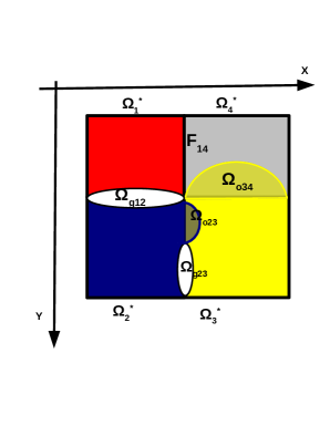
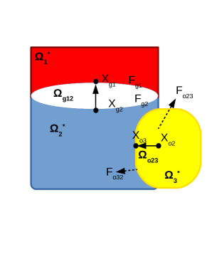
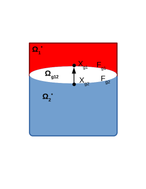
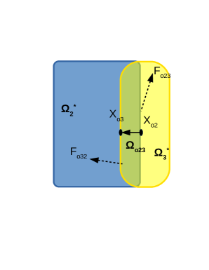
Figure 1: (a) Illustration of a decomposition including gap and overlapping regions, (b) the locations of the diametrically opposite points on gap and overlapping boundaries, (c) a decomposition formed by two patches and a gap region, (d) a decomposition formed by two patches and a overlapping region,

2.6 Gap regions

In this section, we describe a gap region which is located between two patches. Let $\displaystyle\Omega_{1}^{*}$ and $\displaystyle\Omega_{2}^{*}$ be two adjacent patches with the corresponding non-matching interface parametrizations $\displaystyle\mathbf{\Phi}^{*}_{1}:\widehat{\Omega}\rightarrow\Omega^{*}_{1}$ and $\displaystyle\mathbf{\Phi}^{*}_{2}:\widehat{\Omega}\rightarrow\Omega^{*}_{2}$. Further, let $\displaystyle\Omega_{g12}$ to be the gab region such that $\displaystyle\overline{\Omega}_{g12}\subset\overline{\Omega}$ and $\displaystyle|\partial\Omega_{g12}\cap\partial\Omega|=0$, where $\displaystyle|\cdot|$ is the $\displaystyle(d-1)$-dimensional measure. We note that $\displaystyle\overline{\Omega}^{*}_{1}\cup\overline{\Omega}^{*}_{2}\cup\overline{\Omega}_{g12}=\overline{\Omega}_{1}\cup\overline{\Omega}_{2}$. An illustration is given in Figs. 1(b),(c). Without loss of generality, we consider the boundary of the gap region as $\displaystyle\partial\Omega_{g12}=F_{g1}\cup F_{g2}$, with $\displaystyle F_{gi}\subset\Omega^{*}_{i},\,i=1,2$, and we also assume that the face $\displaystyle F_{g2}$ is a simple face, meaning it can be described as the set of points $\displaystyle(x,y,z)$ satisfying

$$0\leq x\leq x_{Mg},{\ }0\leq y\leq\psi_{g2}(x),{\ }0\leq z\leq\phi_{g2}(x,y),$$ (2.19)

where $\displaystyle x_{Mg}$ is a fixed real number, $\displaystyle\psi_{g2}$ and $\displaystyle\phi_{g2}$ are given smooth functions, see Fig. 1(c). As a next step, we need to assign the points $\displaystyle x_{g2}\in F_{g2}$ to the points $\displaystyle x_{g1}\in F_{g1}$. We follow the same ideas as in [16] and [17]. Since $\displaystyle F_{g2}$ is an simple face and $\displaystyle F_{g1}$ is a B-spline surface, due to the fact that it is the the image of some face $\displaystyle\partial\widehat{\Omega}$ under the mapping $\displaystyle\mathbf{\Phi}^{*}_{1}$, we construct a parametrization of $\displaystyle F_{g1}$, lets say $\displaystyle\mathbf{\Phi}_{g21}:F_{g2}\rightarrow F_{g1}$, which is one-to-one and defined as

$$\displaystyle x_{g2}\in F_{g2}\rightarrow\mathbf{\Phi}_{g21}(x_{g2}):=x_{g1}\in F_{g1},\quad\text{with }\quad\mathbf{\Phi}_{g21}(x_{g2})=x_{g2}+\zeta_{g}(x_{g2})n_{F_{g2}},$$ (2.20)

where $\displaystyle n_{F_{g2}}$ is the unit normal vector on $\displaystyle F_{g2}$, see Fig. 1(c), and $\displaystyle\zeta_{g}$ is a B-spline function. The parametrization $\displaystyle\mathbf{\Phi}_{g21}$ defined in (2.20) helps us to assign the diametrically opposite points located on $\displaystyle\partial\Omega_{g12}$, see discussion in [16] and [17]. We are only interested in small gap regions, see below (2.23), and, thereby, if $\displaystyle n_{F_{g1}}$ is the unit normal vector on $\displaystyle F_{g1}$, we can suppose that $\displaystyle n_{F_{g2}}\approx-n_{F_{g1}}$. Consequently, we can define the mapping $\displaystyle\mathbf{\Phi}_{g12}:F_{g1}\rightarrow F_{g2}$ to be

$$\displaystyle\mathbf{\Phi}_{g12}(x_{g1})=x_{g2},{\ }\text{with}\quad\mathbf{\Phi}_{g21}(x_{g2})=x_{g1}.$$ (2.21)

We note that both parametrizations $\displaystyle\mathbf{\Phi}_{g21}$ in (2.20) and $\displaystyle\mathbf{\Phi}_{g12}$ in (2.21) have been constructed under the consideration that one side is planar and $\displaystyle n_{F_{g2}}\approx-n_{F_{g1}}$. As it has been explained in [16] and [17], these parametrizations simplify the calculations and highlight the main ideas of our approach. Furthermore, they lead to an easy materialization of the whole method. In Section 5, we present numerical tests where all the faces of the gap and overlapping regions are curved surfaces. We finally need to quantify the size of the gap. Hence, we introduce the gap width as

$$\displaystyle d_{g}= \displaystyle\max_{x_{g2}\in F_{g2}}|{x_{g2}}-\mathbf{\Phi}_{g21}(x_{g2})|.$$ (2.22)

We focus on gap regions whose width decreases polynomially in $\displaystyle h$, that is,

$$\displaystyle d_{g}\leq \displaystyle h^{\lambda},\quad\text{with some}\quad\lambda\geq 1.$$ (2.23)

2.7 Overlapping regions

We now describe the case of having a overlapping patch decomposition of $\displaystyle\Omega$. Again for simplicity in our analysis, we assume that the overlapping region is formed by involving two patches and it has the same form as the gap regions. Based on (2.10), we suppose that there are two so called physical patches $\displaystyle\Omega_{2}$ and $\displaystyle\Omega_{3}$ that form a decomposition of $\displaystyle\Omega$, i.e.,

$$\displaystyle\overline{\Omega}=\overline{\Omega_{2}}\cup\overline{\Omega_{3}}, \displaystyle\quad\overline{\Omega_{2}}\cap\overline{\Omega_{3}}=\emptyset, \displaystyle{\ }\text{with}{\ }F_{23}=\partial\Omega_{2}\cap\partial\Omega_{3},$$ (2.24)

where $\displaystyle F_{23}$ is the physical interface between $\displaystyle\Omega_{2}$ and $\displaystyle\Omega_{3}$. As we mentioned above, due to an incorrect segmentation procedure, we get two mappings, lets say $\displaystyle\mathbf{\Phi}_{2}^{*}:\widehat{\Omega}\rightarrow\Omega_{2}^{*}$ and $\displaystyle\mathbf{\Phi}_{3}^{*}:\widehat{\Omega}\rightarrow\Omega_{3}^{*}$, which cannot exactly parametrize the two physical patches $\displaystyle{\Omega_{2}}$ and $\displaystyle{\Omega_{3}}$. Let $\displaystyle\Omega_{2}^{*}$ and $\displaystyle\Omega_{3}^{*}$ be the two patches of the corresponding “in-correct” parametrizations, which form an overlapping decomposition of $\displaystyle\Omega$. Let $\displaystyle\Omega_{o23}=\Omega_{2}^{*}\cap\Omega_{3}^{*}$ denote the overlapping region, see Fig. 1(d), and let $\displaystyle F_{oij}=\partial\Omega^{*}_{i}\cap\Omega^{*}_{j},$ with $\displaystyle i,j=2,3$ and $\displaystyle i\neq j$, denote the interior boundary faces of the patches which are related to the overlapping region. Furthermore, let $\displaystyle{n}_{F_{oij}}$ denote the unit exterior normal vector to $\displaystyle F_{oij}$. We assume that $\displaystyle\partial\Omega_{o23}=F_{o23}\cup F_{o32}$. Without loss of generality, we suppose that the following conditions hold: (i) the face $\displaystyle F_{o23}$ coincides with the physical interface, i.e., $\displaystyle F_{o23}=F_{23}$, (ii) the face $\displaystyle F_{o23}$ is a simple face and meaning that it can be described as the set of points $\displaystyle(x,y,z)$ satisfying the inequalities

$$0\leq x\leq x_{M_{o}},{\ }0\leq y\leq\psi_{o2}(x),{\ }0\leq z\leq\phi_{o2}(x,y),$$ (2.25)

where $\displaystyle x_{Mo}$ is a fixed real number, $\displaystyle\psi_{o2}$ and $\displaystyle\phi_{o2}$ are given smooth functions, see Fig. 1(d). We assign the points located on $\displaystyle F_{o23}$ to the opposite points located on $\displaystyle F_{o32}$, by constructing a parametrization for the face $\displaystyle F_{o32}$, i.e., a mapping $\displaystyle\mathbf{\Phi}_{o23}:F_{o23}\rightarrow F_{o32}$. In this way, we consider the face $\displaystyle F_{o32}$ as the image of $\displaystyle F_{o23}$ via the mapping $\displaystyle\mathbf{\Phi}_{o23}$, i.e., $\displaystyle F_{o32}=\mathbf{\Phi}_{o23}(F_{o23})$. Thus, each point $\displaystyle x_{o3}\in F_{o32}$ becomes the image by means of $\displaystyle\mathbf{\Phi}_{o23}$ of a point $\displaystyle x_{o2}\in F_{o23}$, see Fig. 1(e). Using the fact that $\displaystyle F_{o32}$ is a B-spline surface (it is the image of a face of $\displaystyle\partial\widehat{\Omega}$ under the mapping $\displaystyle\mathbf{\Phi}_{3}^{*}$) and since we are interested in overlapping regions with sufficient small widths, see below (2.29), we define the mapping $\displaystyle\mathbf{\Phi}_{o23}:F_{o23}\rightarrow F_{o32}$, as

$$\displaystyle x_{o2}\in F_{o23}\rightarrow\mathbf{\Phi}_{o23}(x_{o2}):=x_{o3}\in F_{o32},\quad\text{with }\quad\mathbf{\Phi}_{o23}(x_{o2})=x_{o2}+\zeta_{o}(x_{o2}){n}_{F_{o23}},$$ (2.26)

where $\displaystyle\zeta_{o}$ is a B-spline and $\displaystyle{n}_{F_{o23}}$ is the unit normal vector on $\displaystyle{F_{o23}}$. In our analysis, we suppose that $\displaystyle{n}_{F_{o23}}\approx-{n}_{F_{o32}}$, and we define the mapping $\displaystyle\mathbf{\Phi}_{o32}:F_{o32}\rightarrow F_{o23}$ as

$$\displaystyle\mathbf{\Phi}_{o32}(x_{o3})=x_{o2},{\ }\text{with}\quad\mathbf{\Phi}_{o23}(x_{o2})=x_{o3}.$$ (2.27)

Finally, we need to quantify the width of the overlapping region $\displaystyle\Omega_{o23}$, defined by

$$\displaystyle d_{o}= \displaystyle\max_{x_{o2}\in F_{o23}}|{x_{o2}}-\mathbf{\Phi}_{o23}(x_{o2})|.$$ (2.28)

We focus on overlapping regions whose distance decreases polynomially in $\displaystyle h$, i.e.,

$$\displaystyle d_{o}\leq \displaystyle h^{\lambda},\quad\text{with some}\quad\lambda\geq 1.$$ (2.29)

2.8 Integrals on the interior faces

Let $\displaystyle F_{1}$ be the simple face of a gap or overlapping region and let $\displaystyle F_{2}$ to be the corresponding opposite boundary faces which admits the parametrization $\displaystyle\mathbf{\Phi}_{12}:F_{1}\rightarrow F_{2}$ written as $\displaystyle\mathbf{\Phi}_{12}(x_{1},x_{2})=(x_{2}(x_{1},y_{1}),y_{2}(x_{1},y_{1}),z_{2}(x_{1},y_{1}))$, which is reduced to $\displaystyle x_{2}=x_{1},\,y_{2}=y_{1}$ and $\displaystyle z_{2}=\Phi_{12,z}(x_{1},x_{2})$, where $\displaystyle\Phi_{12,z}$ is identified by $\displaystyle\zeta_{g}$ in (2.20) or $\displaystyle\zeta_{o}$ in (2.26). For a given smooth function $\displaystyle g$ on $\displaystyle F_{2}$, we have

$$\displaystyle\int_{F_{2}}g(x_{2},y_{2},z_{2})\,d\,F_{2}= \displaystyle\int_{F_{1}}g(x_{1},y_{1},{\Phi}_{12,z}(x_{1},y_{1}))\,\|J\|\,d\,x_{1}\,d\,y_{1},$$ (2.30)

where $\displaystyle\|J\|=\sqrt{1+|\nabla{\Phi}_{12,z}(x_{1},y_{1})|^{2}}$. For simplicity, we will adopt the notation

$$\displaystyle\int_{F_{2}}g\,d\,F_{2}:= \displaystyle\int_{F_{2}}g(x_{2},y_{2},z_{2})\,d\,F_{2},{\ }\text{and}{\ }$$ (2.31a)

$$\displaystyle\int_{F_{1}}g(\mathbf{\Phi}_{12})\,\|J\|\,d\,F_{1}:= \displaystyle\int_{F_{1}}g(x_{1},y_{1},{\Phi}_{12,z}(x_{1},y_{1}))\,\|J\|\,d\,x_{1}\,d\,y_{1}.$$ (2.31b)

Under the regularity of $\displaystyle\mathbf{\Phi}_{12}$, there are positive constants $\displaystyle c_{m}(\|J\|)$ and $\displaystyle C_{M}(\|J\|$ such that

$$\displaystyle C_{m}(\|J\|)\int_{F_{2}}g\,d\,F_{2}\leq\int_{F_{1}}g(\mathbf{\Phi}_{12})\,d\,F_{1}\leq C_{M}(\|J\|)\int_{F_{2}}g\,d\,F_{2}.$$ (2.32)

Furthermore, let us denote the transpose of the Jacobian matrix of mapping $\displaystyle\mathbf{\Phi}_{12}$ evaluated at $\displaystyle\mathbf{x}_{1}\in F_{1}$ by $\displaystyle D^{\intercal}\mathbf{\Phi}_{12}(\mathbf{x}_{1})$, and let $\displaystyle u$ be a smooth function defined on $\displaystyle\Omega$. Then an application of the chain rule yields

$$\displaystyle(\nabla u)\circ\mathbf{\Phi}_{12}=(D^{\intercal}\mathbf{\Phi}_{12})^{-1}\nabla(u\circ\mathbf{\Phi}_{12}).$$ (2.33)

Now, by means of the assumptions imposed on the faces $\displaystyle F_{1}$ and $\displaystyle F_{2}$, we have $\displaystyle n_{F_{1}}=(0,0,1)$. After some elementary calculations, we can find that

$$\displaystyle\int_{F_{1}}\nabla u(\mathbf{\Phi}_{12}(\mathbf{x}_{1}))\cdot n_{F_{1}}\,d\,F_{1}= \displaystyle\int_{F_{1}}\partial_{z}u\circ\mathbf{\Phi}_{12}(\mathbf{x}_{1})\frac{\|J\|}{\|J\|}\,d\,F_{1}\sim\int_{F_{2}}\partial_{z}u\,d\,F_{2}.$$ (2.34)

3 Discontinuous Galerkin IgA schemes for non-matching interfaces

Let $\displaystyle\mathcal{T}^{*}_{H}(\Omega):=\cup_{i=1}^{N}\overline{\Omega_{i}^{*}}$ be an incorrect decomposition of $\displaystyle\Omega$, which may contain overlapping and gap regions between the patches. One has to be careful in constructing the numerical fluxes for the final dG IgA scheme. It is clear from the descriptions above that we cannot directly apply the numerical fluxes of the dG IgA methods, which have been presented in [22] and have been applied on matching parametrized interfaces. However, in [16] and [17], we recently presented dG IgA methods that can be applied on decompositions with gap regions. Since the (exact) boundary data on the boundary of the gaps are not known, we derived appropriate Taylor approximations for them. The Taylor approximations have been constructed using the values of the solution, which are computed on the diametrically opposite points on the gap boundary. These approximations are used to build up the numerical fluxes on the boundary of the gaps. We here follow the same methodology in case of having overlapping regions too.

3.1 Approximations of normal fluxes on the gap boundary

Although dG IgA methods for decompositions including gap regions have been presented by the authors in [16] and [17], we repeat here the main parts for the completeness of the current paper. We present our analysis for the case of two patches described in Subsection 2.7, see also Fig. 1(c). For simplicity of the analysis below, we assume that the face $\displaystyle F_{g2}$ coincides with the physical interface $\displaystyle F_{12}$. This implies that $\displaystyle\Omega_{2}^{*}=\Omega_{2}$. Let $\displaystyle u_{1},\,u_{2}$ and $\displaystyle u_{g12}$ denote the restrictions of the solution $\displaystyle u$ to each domain $\displaystyle\Omega_{1}^{*},\,\Omega_{2}^{*}$ and $\displaystyle\Omega_{g12}$, respectively. The same notation is used to indicate the restrictions for the diffusion coefficient. By the fact that $\displaystyle\Omega_{2}^{*}=\Omega_{2}$, we conclude that $\displaystyle\rho_{g12}=\rho_{1}$. By Assumption 1, we have that $\displaystyle u_{i}\in H^{\ell}(\Omega_{i}^{*}),$ where $\displaystyle\ell\geq 2$, $\displaystyle i=1,2$, and the following interface conditions for the solution $\displaystyle u$ on the two faces of $\displaystyle\partial\Omega_{g12}$, see (2.11),

$$\displaystyle\llbracket u\rrbracket\big{|}_{F_{gi}}=0\quad\text{and}\quad\llbracket\rho\nabla u\rrbracket\cdot n_{F_{gi}}\big{|}_{F_{gi}}=0\,{\ }\text{with}{\ }i=1,2.$$ (3.1)

Let $\displaystyle x_{g2}\in F_{g2}$ and let $\displaystyle x_{g1}\in F_{g1}$ be its corresponding diametrically opposite points such that $\displaystyle x_{g1}=\mathbf{\Phi}_{g21}(x_{g2})$ and $\displaystyle x_{g2}=\mathbf{\Phi}_{g12}(x_{g1}).$ Denoting $\displaystyle r_{g12}=x_{g1}-x_{g2}$ and having $\displaystyle r_{g21}=-r_{g12}$ by means of (2.20) and (2.21), we obtain that the normals are given by $\displaystyle n_{F_{g2}}={r_{g12}}/{|r_{g12}|}$ and $\displaystyle n_{F_{g1}}={r_{g21}}/{|r_{g21}|}$. For convenience, we denote by $\displaystyle\{\rho\}:=({\rho_{g12}+\rho_{i}})/{2}$ the average of the diffusion coefficient across $\displaystyle F_{gi},i=1,2$. Using the interface conditions (3.1), and (2.6), we obtain the formulas

$$\displaystyle\nabla u_{g12}(x_{g2})\cdot n_{F_{g2}}=\nabla u_{1}(x_{g1})\cdot n_{F_{g2}} \displaystyle-\frac{1}{|r_{g12}|}\big{(}R^{2}u_{1}(x_{g2}+s(x_{g1}-x_{g2}))+R^{2}u_{g12}(x_{g1}+s(x_{g2}-x_{g1}))\big{)},\quad$$ (3.2a)

$$\displaystyle-\frac{1}{h}\big{(}u_{2}(x_{g2})-u_{1}(x_{g1})\big{)}= \displaystyle\frac{|r_{g12}|}{h}\nabla u_{g12}(x_{g2})\cdot n_{F_{g2}}+\frac{1}{h}R^{2}u_{g12}(x_{g1}+s(x_{g2}-x_{g1})).$$ (3.2b)

3.2 The modified form on decompositions with gaps

It has been shown in [16] that the solution $\displaystyle u$ of (2.8) under the Assumption 1 and (3.1) satisfies

$$\int_{\Omega_{2}^{*}}\rho_{2}\nabla u\cdot\nabla\phi_{h}\,dx-\int_{\partial\Omega_{2}^{*}\cap\partial\Omega}\rho_{2}\nabla u\cdot n_{\partial\Omega_{2}^{*}}\,\phi_{h}\,d\sigma-\int_{F_{g2}}\{\rho\nabla u\}\cdot n_{F_{g2}}\,\phi_{h}\,d\sigma\\ +\int_{\Omega_{1}^{*}}\rho_{1}\nabla u\cdot\nabla\phi_{h}\,dx-\int_{\partial\Omega_{1}^{*}\cap\partial\Omega}\rho_{1}\nabla u\cdot n_{\partial\Omega_{1}^{*}}\,\phi_{h}\,d\sigma-\int_{F_{g1}}\{\rho\nabla u\}\cdot n_{F_{g1}}\,\phi_{h}\,d\sigma\\ =\int_{\Omega\setminus\overline{\Omega}_{g12}}f\phi_{h}\,dx,\quad\text{for all}{\ }\phi_{h}\in V_{h},$$ (3.3)

where the average of the traces across the interface is denoted by $\displaystyle\{\cdot\}$. The variational form (3.3) plays an essential role in the derivation of the dG IgA scheme. The normal flux terms $\displaystyle\nabla u_{g12}\cdot n_{\partial\Omega_{g12}}$ appearing in (3.3), e.g., $\displaystyle\int_{F_{g2}}\{\rho\nabla u\}\cdot n_{F_{g2}}\phi_{h}\,d\sigma=\int_{F_{g2}}\frac{1}{2}(\rho_{2}\nabla u_{2}+\rho_{g12}\nabla u_{g12})\cdot n_{F_{g2}}\phi_{h}\,d\sigma$, are unknown. They are going to be approximated by means of the normal flux terms $\displaystyle\rho_{2}\nabla u_{2}\cdot n_{F_{g2}}$ and $\displaystyle\rho_{1}\nabla u_{1}\cdot n_{F_{g1}}$. The adaption of these approximations in (3.3) helps us to couple the two different local problems on $\displaystyle\Omega_{2}^{*}$ and $\displaystyle\Omega_{1}^{*}$, and finally, to construct the numerical fluxes on $\displaystyle F_{g1}$ and $\displaystyle F_{g2}$. Using (3.1) and (3.2), we can show that, see [16] and [17],

$$\int_{F_{g2}}\big{(}\frac{\rho_{2}}{2}\nabla u_{2}(x_{g2})+\frac{\rho_{g12}}{2}\nabla u_{g12}(x_{g2})\big{)}\cdot n_{F_{g2}}\phi_{h}\\ =\int_{F_{g2}}\Big{(}\frac{\rho_{2}}{2}\nabla u_{2}(x_{g2})+\frac{\rho_{g12}}{2}\nabla u_{1}(x_{g1})\Big{)}\cdot n_{F_{g2}}\phi_{h}-\frac{\{\rho\}}{h}\big{(}u_{2}(x_{g2})-u_{1}(x_{g1})\big{)}\phi_{h}\,d\sigma\\ -\int_{F_{g2}}\Big{(}\frac{\rho_{g12}}{2|r_{g12}|}R^{2}u_{g12}(x_{g1}+s(x_{g2}-x_{g1}))+\frac{\rho_{g12}}{2|r_{g12}|}R^{2}u_{g12}(x_{g2}+s(x_{g1}-x_{g2}))\Big{)}\phi_{h}\,d\sigma\\ +\int_{F_{g2}}\frac{\{\rho\}}{h}\Big{(}|r_{g12}|\nabla u_{g12}\cdot n_{F_{g2}}+R^{2}u_{g12}(x_{g1}+s(x_{g2}-x_{g1}))\Big{)}\phi_{h}\,d\sigma,$$ (3.4)

and similarly

$$\int_{F_{g1}}\Big{(}\frac{\rho_{1}}{2}\nabla u_{1}(x_{g1})+\frac{\rho_{g12}}{2}\nabla u_{g12}(x_{g1})\Big{)}\cdot n_{F_{g1}}\phi_{h}-\frac{\{\rho\}}{h}\llbracket u(x_{g1})\rrbracket\phi_{h}\,d\sigma\\ =\int_{F_{g1}}\Big{(}\frac{\rho_{1}}{2}\nabla u_{1}(x_{g1})+\frac{\rho_{2}}{2}\nabla u_{2}(x_{g2})\Big{)}\cdot n_{F_{g1}}\phi_{h}-\frac{\{\rho\}}{h}\big{(}u_{1}(x_{g1})-u_{2}(x_{g2})\big{)}\phi_{h}\,d\sigma\\ -\int_{F_{g1}}\Big{(}\frac{\rho_{g12}}{2|r_{g21}|}R^{2}u_{g12}(x_{g2}+s(x_{g1}-x_{g2}))+\frac{\rho_{g12}}{2|r_{g21}|}R^{2}u_{2}(x_{g1}+s(x_{g2}-x_{g1}))\Big{)}\phi_{h}\,d\sigma\\ +\int_{F_{g1}}\frac{\{\rho\}}{h}\Big{(}|r_{g21}|\nabla u_{g12}\cdot n_{F_{g1}}+R^{2}u_{g12}(x_{g2}+s(x_{g1}-x_{g2}))\Big{)}\phi_{h}\,d\sigma.$$ (3.5)

Inserting (3.4) and (3.5) into (3.3), and after few calculations, we obtain the following modified form

$$\sum_{i=1}^{2}\int_{\Omega_{i}^{*}}\rho_{i}\nabla u\cdot\nabla\phi_{h}\,dx-\int_{\partial\Omega_{i}^{*}\cap\partial\Omega}\rho_{i}\nabla u\cdot n_{\partial\Omega_{i}^{*}}\phi_{h}\,d\sigma-\int_{F_{g2}}\Big{(}\frac{\rho_{2}}{2}\nabla u_{2}+\frac{\rho_{g12}}{2}\nabla u_{1}\Big{)}\cdot n_{F_{g2}}\phi_{h}-\frac{\{\rho\}}{h}\big{(}u_{2}-u_{1}\big{)}\phi_{h}\,d\sigma\\ +\int_{F_{g2}}\Big{(}\frac{\rho_{g12}}{2|r_{g12}|}R^{2}u_{g12}(x_{g1}+s(x_{g2}-x_{g1}))+\frac{\rho_{g12}}{2|r_{g12}|}R^{2}u_{g12}(x_{g2}+s(x_{g1}-x_{g2}))\Big{)}\phi_{h}\,d\sigma\\ -\int_{F_{g2}}\frac{\{\rho\}}{h}\Big{(}|r_{g12}|\nabla u_{g12}\cdot n_{F_{g2}}+R^{2}u_{g12}(x_{g1}+s(x_{g2}-x_{g1}))\Big{)}\phi_{h}\,d\sigma\\ -\int_{F_{g1}}\Big{(}\frac{\rho_{1}}{2}\nabla u_{1}+\frac{\rho_{2}}{2}\nabla u_{2}\Big{)}\cdot n_{F_{g1}}\phi_{h}-\frac{\{\rho\}}{h}\big{(}u_{1}-u_{2}\big{)}\phi_{h}\,d\sigma\\ +\int_{F_{g1}}\Big{(}\frac{\rho_{g12}}{2|r_{g21}|}R^{2}u_{g12}(x_{g2}+s(x_{g1}-x_{g2}))+\frac{\rho_{g12}}{2|r_{g21}|}R^{2}u_{2}(x_{g1}+s(x_{g2}-x_{g1}))\Big{)}\phi_{h}\,d\sigma\\ -\int_{F_{g1}}\frac{\{\rho\}}{h}\Big{(}|r_{g21}|\nabla u_{g12}\cdot n_{F_{g1}}+R^{2}u_{g12}(x_{g2}+s(x_{g1}-x_{g2}))\Big{)}\phi_{h}\,d\sigma=\int_{\Omega\setminus\overline{\Omega}_{g12}}f\phi_{h}\,dx,{\ }\text{for all}{\ }\phi_{h}\in V_{h}.$$ (3.6)

3.3 The local problems on overlapping regions

For the sake of simplicity, we present the analysis for the case of having only two patches. Let $\displaystyle\{\Omega_{i}\}_{i=2}^{N=3}$ be a physical non-overlapping decomposition of $\displaystyle\Omega$ with the interface $\displaystyle F_{23}$, see (2.10). Then (2.13) is reduced to

$$\displaystyle\sum_{i=2,3}\int_{\Omega_{i}}\rho_{i}(x)\nabla u_{i}\nabla\phi\,dx-\int_{F_{23}}\llbracket\rho\nabla u\phi\rrbracket\cdot n_{F_{23}}\,d\sigma=\sum_{i=2,3}\int_{\Omega_{i}}f\phi\,dx,\quad\text{for all}{\ }\phi\in H^{1}_{0}(\Omega),$$ (3.7)

where the sub-index $\displaystyle i$ denotes the restriction of functions to the patch $\displaystyle\Omega_{i}$ for $\displaystyle i=2,3$. Let $\displaystyle\Omega_{i}^{*}$, $\displaystyle i=2,3$, be two patches that form an overlapping decomposition of $\displaystyle\Omega$, with the overlapping region $\displaystyle\Omega_{o23}=\Omega_{2}^{*}\cap\Omega_{3}^{*}$, see Fig. 1(d). Let $\displaystyle F_{oij}=\partial\Omega_{i}^{*}\cap\Omega_{j}^{*},\,i,j=2,3$, $\displaystyle i\neq j$, be the interior faces that define $\displaystyle\partial\Omega_{o23}$. Without loss of generality, we suppose that $\displaystyle F_{o23}=F_{23}$, see (3.7), which in turn implies that $\displaystyle\Omega_{2}^{*}=\Omega_{2}$ and $\displaystyle\Omega_{3}^{*}=\Omega_{3}\cup\Omega_{o23}$, see Figs. 1(d). We can view $\displaystyle\{\Omega_{i}^{*}\}_{i=2,3}$ as an extension of the physical decomposition $\displaystyle\{\Omega_{i}\}_{i=2,3}$ by $\displaystyle\Omega_{o23}$. To proceed on decomposition $\displaystyle\{\Omega_{i}^{*}\}_{i=2,3}$, we consider the following perturbed local problems on $\displaystyle\Omega_{2}^{*}$ and $\displaystyle\Omega_{3}^{*}$. The sub-index indicates the restrictions of the quantities to the patches, and $\displaystyle u_{o,2}^{*}$ will denote the restriction of $\displaystyle u_{2}^{*}$ to $\displaystyle\Omega_{o23}$, and $\displaystyle u_{o,3}^{*}$ the corresponding restriction of $\displaystyle u_{3}^{*}$ to $\displaystyle\Omega_{o23}$. Given the source function $\displaystyle f$ and Dirichlet data $\displaystyle u_{D}$ we consider the local problems: find $\displaystyle u_{2}^{*}\in H^{1}(\Omega_{2}^{*})$ and $\displaystyle u_{3}^{*}\in H^{1}(\Omega_{3}^{*})$ such that

$$\displaystyle\begin{cases}a^{(2)}_{o,\rho_{2}}(u_{2}^{*},\phi_{2})=l^{(2)}_{f}(\phi_{2}),\quad\text{for all}\;\phi_{2}\in H^{1}_{0}(\Omega_{2}^{*})\\ u_{2}^{*}=u_{3}^{*},\,\text{on}\,F_{o23},\quad u_{2}^{*}=u_{D},\,\text{on}\,\partial\Omega_{2}^{*}\cap\partial\Omega,\\ \text{where }{\ }a^{(2)}_{o,\rho_{2}}(u_{2}^{*},\phi_{2})=\int_{\Omega_{2}^{*}}\rho_{2}\nabla u_{2}^{*}\cdot\nabla\phi_{2}\,dx-\int_{\partial\Omega_{2}^{*}\cap\partial\Omega}\rho_{2}\nabla u_{2}^{*}\cdot n_{\partial\Omega_{2}^{*}}\phi_{2}\,d\sigma-\int_{F_{o23}}\rho_{2}\nabla u_{2}^{*}\cdot n_{F_{o23}}\phi_{2}\,d\sigma,\\ \text{and}\quad l^{(2)}_{f}(\phi_{2})=\int_{\Omega_{2}^{*}}f\phi_{2}\,dx,\end{cases}$$ (3.8a)

$$\displaystyle\begin{cases}a^{(3)}_{o,\rho_{3}}(u_{3}^{*},\phi_{3})=l^{(3)}_{f}(\phi_{3}),\quad\text{for all}\;\phi_{3}\in H^{1}_{0}(\Omega_{3}^{*})\\ u_{3}^{*}=u_{2}^{*},\,\text{on}\,F_{o32},\quad u_{3}^{*}=u_{D},\,\text{on}\,\partial\Omega_{3}^{*}\cap\partial\Omega,\\ \text{where}\quad a^{(3)}_{o,\rho_{3}}(u_{3}^{*},\phi_{3})=\int_{\Omega_{3}^{*}}\rho_{3}\nabla u_{3}^{*}\cdot\nabla\phi_{3}\,dx-\int_{\partial\Omega_{3}^{*}\cap\partial\Omega}\rho_{3}\nabla u_{3}^{*}\cdot n_{\partial\Omega_{3}}\phi_{3}\,d\sigma-\int_{F_{o32}}\rho_{3}\nabla u_{3}^{*}\cdot n_{F_{o32}}\phi_{3}\,d\sigma,\\ \text{and}\quad l^{(3)}_{f}(\phi_{3})=\int_{\Omega_{3}^{*}}f^{*}\phi_{3}\,dx.\end{cases}$$ (3.8b)

We note that (3.8b) is not equivalent to (3.7). Furthermore, in (3.8), we set $\displaystyle\rho_{o23}=\rho_{3}$. In general, the artificial problems defined in (3.8) are not consistent with the original problem (3.7). Since the B-spline spaces are defined on the overlapping domains $\displaystyle\Omega^{*}_{2}$ and $\displaystyle\Omega_{3}^{*}$, the dG IgA scheme will be determined based on variational problems (3.8). In correspondence with Assumption 1, we make the following assumption.

Assumption 5

Let $\displaystyle\ell\geq 2$ be an integer. For the solutions of (3.8), we assume that $\displaystyle u_{3}^{*}\in H^{\ell}(\Omega_{3}^{*})$ and $\displaystyle u_{2}^{*}\in H^{\ell}(\Omega_{2})$.

The interface conditions given in (3.8) and (2.11), Assumption 5 and Assumption 1 yield

$$\displaystyle\begin{cases}u_{2}=u_{2}^{*},&\quad\text{on}\quad\Omega_{2},\\ u_{3}=u_{3}^{*},&\quad\text{on}\quad\Omega_{3},\\ (\rho_{3}\nabla u^{*}_{o,3}-\rho_{3}\nabla u_{3})\cdot n_{F_{o23}}=(\rho_{2}\nabla u_{o,2}^{*}-\rho_{3}\nabla u_{3}^{*})\cdot n_{F_{o23}}=0,&\quad\text{on}\quad F_{o23}.\end{cases}$$ (3.9)

Now, we show that, in the limit case of $\displaystyle d_{o}\rightarrow 0$, we can recover the physical continuity conditions across the interfaces, see (2.11). If $\displaystyle x_{o2}$ and $\displaystyle x_{o3}$ are two opposite points on $\displaystyle\partial\Omega_{o23}$, see Fig. 1(d), then by (2.28) we have that $\displaystyle|x_{o2}-x_{o3}|\leq d_{o}$, and, consequently, we have

$$\displaystyle|u_{3}^{*}(x_{o2})-u_{2}^{*}(x_{o3})|=|u_{3}^{*}(x_{o2})-u_{3}^{*}(x_{o3})|{\xrightarrow{d_{o}\rightarrow 0}}0,$$ (3.10)

due to the continuity of $\displaystyle u_{3}^{*}$.

Proposition 1

Let $\displaystyle\Omega_{o23}$ be the overlapping region with $\displaystyle\partial\Omega_{o23}=F_{o23}\cup F_{o32}$, and let the parametrizations $\displaystyle\mathbf{\Phi}_{o23}$ and $\displaystyle\mathbf{\Phi}_{o32}$ be defined as in (2.26) and in (2.27). Then there exists a positive constant $\displaystyle C_{1}$ such that

$$\displaystyle\Big{|}\int_{F_{o32}}\rho_{3}\nabla u^{*}_{o,3}\cdot n_{F_{o23}}\,dF_{o32}-\int_{F_{o32}}\rho_{3}\nabla u^{*}_{o,3}\cdot n_{F_{o32}}\,dF_{o32}\Big{|}\leq \displaystyle C_{1}d_{o}\|\rho_{3}\nabla u^{*}_{o,3}\|_{L^{2}(F_{o32})},$$ (3.11)

where the normal vectors $\displaystyle n_{F_{o23}}$ and $\displaystyle n_{F_{o32}}$ are defined towards the same direction.

Proof

The proof is given in [16] for the case of gap regions. The same arguments can be applied for the case under consideration. $\displaystyle\hfill\blacksquare$

Lemma 1

Let Assumptions 1 and 5 hold. Then there is a positive constant
$\displaystyle C(\|u^{*}_{o,3}\|_{W^{2,2}(\Omega_{o23})},\|\nabla u^{*}_{o,3}\|_{L^{2}(F_{o23})})$ independent of $\displaystyle h$, such that

$$\displaystyle\|(\rho_{3}\nabla u^{*}_{o,3}-\rho_{2}\nabla u_{o,2}^{*})\cdot n_{F_{o32}}\|_{L^{2}(F_{o32})} \displaystyle\leq Cd_{o}.$$ (3.12)

Proof

Let $\displaystyle x_{o3}=\mathbf{\Phi}_{o23}(x_{o2})$. Using the interface conditions (2.11) and (3.9) as well as (2.30), we get

$$\|(\rho_{3}\nabla u^{*}_{o,3}-\rho_{2}\nabla u_{o,2}^{*})\cdot n_{F_{o32}}\|^{2}_{L^{2}(F_{o32})}\leq 2\int_{F_{o23}}\big{(}(\rho_{3}\nabla u^{*}_{o,3}(\mathbf{\Phi}_{o23})-\rho_{2}\nabla u_{o,2}^{*}(\mathbf{\Phi}_{o23}))\cdot n_{F_{o32}}\big{)}^{2}\|J\|\,d\,F_{o23}\\ \leq 4\int_{F_{o23}}\Big{(}\big{(}\rho_{3}\nabla u^{*}_{o,3}(\mathbf{\Phi}_{o23})\cdot n_{F_{o32}}-\rho_{3}\nabla u_{3}(x_{o2})\cdot n_{F_{o23}}\big{)}^{2}+\big{(}\rho_{2}\nabla u_{o,2}^{*}(\mathbf{\Phi}_{o23})\cdot n_{F_{o32}}-\rho_{2}\nabla u_{2}(x_{o2})\cdot n_{F_{o23}}\big{)}^{2}\Big{)}\|J\|\,d\,F_{o23}\\ \leq 4\int_{F_{o23}}\Big{(}\big{(}\rho_{3}\nabla u^{*}_{o,3}(\mathbf{\Phi}_{o23})\cdot n_{F_{o32}}-\rho_{3}\nabla u^{*}_{o,3}(x_{o2})\cdot n_{F_{o23}}\big{)}^{2}+\big{(}\rho_{2}\nabla u_{2}(\mathbf{\Phi}_{o23})\cdot n_{F_{o32}}-\rho_{2}\nabla u_{2}(x_{o2})\cdot n_{F_{o23}}\big{)}^{2}\Big{)}\|J\|\,d\,F_{o23}\\ \leq 8\int_{F_{o23}}\Big{(}\rho_{3}^{2}\big{(}(\nabla u^{*}_{o,3}(\mathbf{\Phi}_{o23})-\nabla u^{*}_{o,3}(x_{o2}))\cdot n_{F_{o32}}+\nabla u^{*}_{o,3}(x_{o2})\cdot(n_{F_{o32}}-n_{F_{o23}})\big{)}^{2}+\\ \qquad\rho_{2}^{2}\big{(}(\nabla u_{2}(\mathbf{\Phi}_{o23})-\nabla u_{2}(x_{o2}))\cdot n_{F_{o32}}+\nabla u_{2}(x_{o2})\cdot(n_{F_{o32}}-n_{F_{o23}})\big{)}^{2}\Big{)}\|J\|\,d\,F_{o23}\\ \leq 8\max(\rho_{3}^{2},\rho^{2}_{2})(T_{1}+T_{2}+T_{3}+T_{4}).\qquad$$

We now proceed to bound each of the $\displaystyle T_{i},\,i=1,\ldots,4$ terms. For the term $\displaystyle T_{1}$, we have

$$\displaystyle T_{1}\leq \displaystyle\int_{F_{o32}}\Bigg{|}\int_{x_{o2}}^{\mathbf{\Phi}_{o23}}\Big{(}\frac{\partial}{\partial t}\nabla u^{*}_{o,3}(t)\Big{)}\,dt\Bigg{|}^{2}\,d\,F_{o23}\leq d_{o}\,\int_{F_{o32}}\int_{x_{o2}}^{\mathbf{\Phi}_{o23}}\Big{(}\frac{\partial}{\partial t}\nabla u^{*}_{o,3}(t)\Big{)}^{2}\,dt\,d\,F_{o23}$$ (3.13)

$$\displaystyle\leq \displaystyle d_{o}\|u^{*}_{o,3}\|_{W^{2,2}(\Omega_{o23})}.$$

For the term $\displaystyle T_{2}$, we use (3.11) and we immediately have $\displaystyle T_{2}\leq Cd_{o}^{2}\,\|\nabla u^{*}_{o,3}\|^{2}_{L^{2}(F_{o23})}.$ The terms $\displaystyle T_{3}$ and $\displaystyle T_{4}$ can be analogously bounded. Gathering the previous bounds, we derive (3.12). $\displaystyle\hfill\blacksquare$

Thus, by (3.9), (3.10) and (3.12), we infer that the conditions (2.11) are recovered as $\displaystyle d_{o}\rightarrow 0$.

Remark 3

Under the assumption $\displaystyle n_{F_{o32}}\approx-n_{F_{o23}}$, the terms $\displaystyle T_{2}$ and $\displaystyle T_{4}$ can be ignored from the previous estimates.

3.4 Approximations of normal fluxes and the modified form on overlapping regions

The normal fluxes in (3.8) on the faces $\displaystyle F_{o23}$ and $\displaystyle F_{o32}$ of the overlapping boundary, must be appropriately modified in order to couple the two local problems. Then, we use these modifications in order to introduce Taylor approximations of the normal fluxes and to construct finally the numerical fluxes on $\displaystyle\partial\Omega_{23}$, which in turn couple the local patch-wise discrete problems.

3.4.1 Approximations of normal fluxes by Taylor expansions.

Let $\displaystyle x_{o2}\in F_{o23}$ and $\displaystyle x_{o3}\in F_{o32}$ be such that $\displaystyle x_{o3}=\mathbf{\Phi}_{o23}(x_{o2})$. Denoting $\displaystyle r_{o23}=x_{o2}-x_{o3}$ and using the assumption that $\displaystyle r_{o23}=-r_{o32}$, we obtain that $\displaystyle n_{F_{o23}}=\frac{r_{o23}}{|r_{o23}|}=-n_{F_{o32}}$. Using the interface conditions of (3.8), (3.9) and (2.6), we obtain the formulas

$$\displaystyle\nabla u^{*}_{3}(x_{o3})\cdot n_{F_{o23}}=\nabla u^{*}_{2}(x_{o2})\cdot n_{F_{o23}} \displaystyle-\frac{1}{|r_{o23}|}\big{(}R^{2}u^{*}_{2}(x_{o3}+s(x_{o2}-x_{o3}))+R^{2}u^{*}_{3}(x_{o2}+s(x_{o3}-x_{o2}))\big{)}$$ (3.14a)

$$\displaystyle-\frac{1}{h}\big{(}u^{*}_{2}(x_{o3})-u^{*}_{3}(x_{o2})\big{)}= \displaystyle\frac{|r_{o23}|}{h}\nabla u^{*}_{2}(x_{o3})\cdot n_{F_{o3}}+\frac{1}{h}R^{2}u^{*}_{2}(x_{o2}+s(x_{o3}-x_{o2})).$$ (3.14b)

3.4.2 The modified form.

To treat the overlapping nature of the IgA parametrizations, we use the bilinear forms in (3.8), the interface conditions given in (3.9), the fact that $\displaystyle F_{o23}=F_{23}$ and $\displaystyle\Omega_{2}^{*}=\Omega_{2}$, and obtain

$$\displaystyle a^{(2)}_{o,\rho_{2}}(u_{2}^{*},\phi_{h})+a^{(3)}_{o,\rho_{3}}(u_{3}^{*},\phi_{h})=$$

$$\displaystyle\int_{\Omega_{2}^{*}}\rho_{2}\nabla u_{2}^{*}\cdot\nabla\phi_{h}\,dx- \displaystyle\int_{\partial\Omega_{2}^{*}\cap\partial\Omega}\rho_{2}\nabla u_{2}^{*}\cdot n_{\partial\Omega_{2}^{*}}\phi_{h}\,d\sigma$$

$$\displaystyle-\int_{F_{o23}}\frac{1}{2}\big{(}\rho_{2}\nabla u_{2}^{*}(x_{o2})+\rho_{2}\nabla u_{2}^{*}(x_{o2})\big{)}\cdot n_{F_{o23}}\phi_{h}-\frac{\{\rho\}}{h}(u^{*}_{2}(x_{o2})-u^{*}_{2}(x_{o2}))\phi_{h}\,d\sigma$$

$$\displaystyle+\int_{\Omega_{3}^{*}}\rho_{3}\nabla u_{3}^{*}\cdot\nabla\phi_{h}\,dx- \displaystyle\int_{\partial\Omega_{3}^{*}\cap\partial\Omega}\rho_{3}\nabla u_{3}^{*}\cdot n_{\partial\Omega_{3}^{*}}\phi_{h}\,d\sigma$$

$$\displaystyle- \displaystyle\int_{F_{o32}}\frac{1}{2}\big{(}{\rho_{3}}\nabla u_{3}^{*}(x_{o3})+{\rho_{3}}\nabla u_{3}^{*}(x_{o3})\big{)}\cdot n_{F_{o32}}\phi_{h}-\frac{\{\rho\}}{h}(u_{3}^{*}(x_{o3})-u_{3}^{*}(x_{o3}))\phi_{h}\,d\sigma$$

$$\displaystyle= \displaystyle\int_{\Omega_{2}^{*}}f\phi_{h}\,dx+\int_{\Omega_{3}^{*}}f\phi_{h}\,dx,\quad\text{for all}\quad\phi_{h}\in V_{h}.$$ (3.15)

Using in (3.4.2) the continuity conditions across the faces that are given in (3.8), consequently employing the Taylor expansions (3.14) and adopting the notation $\displaystyle x_{o3}:=\mathbf{\Phi}_{o23}(x_{o2})$, $\displaystyle x_{o2}:=\mathbf{\Phi}_{o32}(x_{o3})$, we get

$$\int_{\Omega_{2}^{*}}\rho_{2}\nabla u_{2}^{*}\cdot\nabla\phi_{h}\,dx-\int_{\partial\Omega_{2}^{*}\cap\partial\Omega}\rho_{2}\nabla u_{2}^{*}\cdot n_{\partial\Omega_{2}^{*}}\phi_{h}\,d\sigma+\int_{\Omega_{3}^{*}}\rho_{3}\nabla u_{3}^{*}\cdot\nabla\phi_{h}\,dx-\int_{\partial\Omega_{3}^{*}\cap\partial\Omega}\rho_{3}\nabla u_{3}^{*}\cdot n_{\partial\Omega_{3}^{*}}\phi_{h}\,d\sigma\\ -\int_{F_{o23}}\frac{1}{2}\big{(}\rho_{2}\nabla u_{2}^{*}(x_{o2})+\rho_{3}\nabla u_{3}^{*}(x_{o3})\big{)}\cdot n_{F_{o23}}\phi_{h}+\frac{\rho_{2}}{2|r_{o23}|}\big{(}R^{2}u^{*}_{2}(x_{o3}+s(x_{o2}-x_{o3}))+R^{2}u^{*}_{3}(x_{o2}+s(x_{o3}-x_{o2}))\big{)}\phi_{h}\\ -\frac{\{\rho\}}{h}(u_{2}^{*}(x_{o2})-u_{3}^{*}(x_{o3}))\phi_{h}+\frac{\{\rho\}}{h}\big{(}|r_{o23}|\nabla u^{*}_{3}(x_{o2})\cdot n_{F_{o23}}+R^{2}u^{*}_{3}(x_{o3}+s(x_{o2}-x_{o3}))\big{)}\phi_{h}\,d\sigma\\ -\int_{F_{o32}}\frac{1}{2}\big{(}\rho_{3}\nabla u_{3}^{*}(x_{o3})+\rho_{2}\nabla u_{2}^{*}(x_{o2})\big{)}\cdot n_{F_{o32}}\phi_{h}+\frac{\rho_{3}}{2|r_{o32}|}\big{(}R^{2}u^{*}_{2}(x_{o3}+s(x_{o2}-x_{o3}))+R^{2}u^{*}_{3}(x_{o2}+s(x_{o3}-x_{o2}))\big{)}\phi_{h}\\ -\frac{\{\rho\}}{h}(u_{3}^{*}(x_{o3})-u_{2}^{*}(x_{o2}))\phi_{h}+\frac{\{\rho\}}{h}\big{(}|r_{o32}|\nabla u_{2}^{*}(x_{o3})\cdot n_{F_{o32}}-R^{2}u^{*}_{2}(x_{o2}+s(x_{o3}-x_{o2}))\big{)}\phi_{h}\,d\sigma\\ =\int_{\Omega_{2}^{*}}f\phi_{h}\,dx+\int_{\Omega_{3}^{*}}f\phi_{h}\,dx,\quad\text{for all}\quad\phi_{h}\in V_{h}.$$ (3.16)

3.5 The consistency error.

As we pointed out above, due to the overlapping of the diffusion coefficient on $\displaystyle\Omega_{o23}$ the solution $\displaystyle u_{3}^{*}|_{\Omega_{o23}}$ is different from the physical solution $\displaystyle u|_{\Omega_{o23}}$ given by (3.7). In particular, by the interface conditions (3.9), we have

$$\displaystyle a^{(3)}_{o,\rho_{3}}(u_{3}^{*},\phi_{3})= \displaystyle\int_{\Omega_{3}^{*}}\rho_{3}\nabla u_{3}^{*}\cdot\nabla\phi_{3}\,dx-\int_{\partial\Omega_{3}^{*}\cap\partial\Omega}\rho_{3}\nabla u_{3}^{*}\cdot n_{\partial\Omega_{3}}\phi_{3}\,d\sigma-\int_{F_{o32}}\rho_{3}\nabla u_{3}^{*}\cdot n_{F_{o32}}\phi_{3}\,d\sigma$$

$$\displaystyle= \displaystyle\int_{\Omega_{o23}}\rho_{3}\nabla u_{o,3}^{*}\cdot\nabla\phi_{3}\,dx-\int_{F_{o23}}{\rho_{3}}\nabla u_{o,3}^{*}\cdot n_{F_{o23}}\phi_{3}\,d\sigma-\int_{F_{o23}}{\rho_{3}}\nabla u_{3}^{*}\cdot(-n_{F_{o23}})\phi_{3}\,d\sigma$$

$$\displaystyle- \displaystyle\int_{F_{o32}}{\rho_{3}}\nabla u_{o,3}^{*}\cdot n_{F_{o32}}\phi_{3}\,d\sigma+\int_{\Omega_{3}}\rho_{3}\nabla u^{*}_{3}\cdot\nabla\phi_{3}\,dx-\int_{\partial\Omega_{3}^{*}\cap\partial\Omega}\rho\nabla u_{3}^{*}\cdot n_{\partial\Omega_{3}^{*}}\phi_{3}\,d\sigma$$

$$\displaystyle= \displaystyle\int_{\Omega_{3}^{*}}f\phi_{3}\,dx,\quad\text{for}\quad\phi_{3}\in W^{1,2}_{0}(\Omega_{3}^{*}).$$ (3.17)

The physical relevant form with $\displaystyle\rho=\rho_{2}$ on $\displaystyle\Omega_{o23}$ is

$$\displaystyle a^{(3)}_{o,\rho_{2}}(u,\phi_{3})= \displaystyle\int_{\Omega_{o23}}\rho_{2}\nabla u_{o,2}^{*}\cdot\nabla\phi_{3}\,dx-\int_{F_{o23}}{\rho_{2}}\nabla u_{o,2}^{*}\cdot n_{F_{o23}}\phi_{3}\,d\sigma-\int_{F_{o23}}{\rho_{3}}\nabla u_{3}\cdot(-n_{F_{o23}})\phi_{3}\,d\sigma$$

$$\displaystyle- \displaystyle\int_{F_{o32}}{\rho_{2}}\nabla u_{o,2}^{*}\cdot n_{F_{o32}}\phi_{3}\,d\sigma+\int_{\Omega_{3}}\rho_{3}\nabla u_{3}\cdot\nabla\phi_{3}\,dx-\int_{\partial\Omega_{3}^{*}\cap\partial\Omega}\rho\nabla u_{3}\cdot n_{\partial\Omega_{3}^{*}}\phi_{3}\,d\sigma$$

$$\displaystyle= \displaystyle\int_{\Omega_{3}^{*}}f\phi_{3}\,dx,\quad\text{for}\quad\phi_{3}\in W^{1,2}_{0}(\Omega_{3}^{*}).$$ (3.18)

Now, by the construction of the local problems, it holds that $\displaystyle u_{o,2}^{*}=u_{2}|_{\Omega_{o23}}$, where $\displaystyle u_{2}|_{\Omega_{o23}}$ is the restriction of solution $\displaystyle u$ given by (3.7) to $\displaystyle{\Omega_{o23}}$, and as well it holds $\displaystyle u_{3}|_{\Omega_{3}}=u_{3}^{*}|_{\Omega_{3}}$. Therefore, from (3.5) and (3.5), we obtain that the difference $\displaystyle\rho_{2}\nabla u_{2}-\rho_{3}\nabla u^{*}_{o,3}$ on $\displaystyle\Omega_{o23}$ satisfies $\displaystyle\int_{\Omega_{o23}}(\rho_{2}\nabla u_{2}-\rho_{3}\nabla u^{*}_{o,3})\cdot\nabla\phi_{3}\,dx=0,$ and taking $\displaystyle\phi_{3}=(\rho_{2}u_{2}-\rho_{3}u^{*}_{o,3})$, we obtain $\displaystyle\int_{\Omega_{o23}}\big{|}\rho_{2}\nabla u_{2}-\rho_{3}\nabla u^{*}_{o,3}\big{|}^{2}\,dx=0.$ Also, it follows by (3.8) that

$$\displaystyle\int_{F_{o32}}\frac{\{\rho\}}{h}(u_{2}(x_{o3})-u_{o,3}^{*}(x_{o3}))^{2}\,d\sigma=\int_{F_{o23}}\frac{\{\rho\}}{h}(u_{2}(x_{o2})-u_{o,3}^{*}(x_{o2}))^{2}\,d\sigma=0.$$ (3.19)

and thus

$$\displaystyle\int_{\Omega_{o23}}\big{|}\rho_{2}\nabla u_{2}-\rho_{3}\nabla u^{*}_{o,3}\big{|}^{2}\,dx+\frac{\{\rho\}}{h}\Big{(}\int_{F_{o32}}(u_{2}(x_{o3})-u_{o,3}^{*}(x_{o3}))^{2}\,d\sigma+\int_{F_{o23}}(u_{o,3}^{*}(x_{o2})-u_{2}(x_{o2}))^{2}\,d\sigma\Big{)}=0.$$ (3.20)

————————————————————————————————–

3.6 The dG IgA form on general decompositions

In the previous section, relation (3.6) has been derived for a decomposition consisting of two patches $\displaystyle\Omega_{1}^{*}$ and $\displaystyle\Omega_{2}^{*}$, that are separated by the gap region $\displaystyle\Omega_{g12}$. Working in the same spirit, the form (3.16) has been derived for a decomposition of $\displaystyle\Omega$ formed by two overlapping patches $\displaystyle\Omega_{2}^{*}$ and $\displaystyle\Omega_{3}^{*}$. It is clear that for a general decomposition $\displaystyle\mathcal{T}^{*}_{H}(\Omega):=\cup^{N}_{i=1}\Omega^{*}_{i}$ of $\displaystyle\Omega$ that includes gap and overlapping regions, similar expressions can be derived by defining the corresponding Taylor expansions. Below, we describe the proposed dG IgA scheme for a general decomposition.

So far, we denoted the restrictions of the solution of the perturbed problems on each $\displaystyle\Omega_{i}^{*}$ by $\displaystyle u_{i}^{*}$. That was useful because the solution of the perturbed problem does not coincide with the solution of (2.8). In the following sections, we aim at avoiding lengthy formulas with complicated notations. Hence, we will denote the solution obtained on $\displaystyle\mathcal{T}^{*}_{H}(\Omega)$ by $\displaystyle u$, and its restriction on every patch $\displaystyle\Omega^{*}_{i}$ by $\displaystyle u_{i}$, independent of having gaps, overlaps or matching interfaces. The corresponding diffusion coefficient is denoted by $\displaystyle\rho_{i}$.
Let $\displaystyle\ell\geq 2$ be an integer and let $\displaystyle\mathcal{F}^{*}$ be the set of all the interior faces of $\displaystyle\{\partial\Omega_{i}^{*}\}_{i=1}^{N}$. In association with $\displaystyle\mathcal{T}^{*}_{H}(\Omega)$ and $\displaystyle\mathcal{F}^{*}$, we introduce the space

$$\displaystyle V^{*}:=\{v\in H^{\ell}(\Omega^{*}_{i}),\,\text{for}\,i=1,\ldots,N:\llbracket v\rrbracket|_{F}=0\,\text{for all}\,F\in\mathcal{F}^{*}\},$$ (3.21)

where $\displaystyle\llbracket v\rrbracket|_{F}$ denotes the jump of $\displaystyle v$ across $\displaystyle F$. By the definition of the patch-wise solutions, see e.g. (3.1) and (3.8), we can assume that $\displaystyle u\in V^{*}$. In order to proceed with our analysis, we first define the dG-norm $\displaystyle\|.\|_{dG}$ associated with $\displaystyle\mathcal{T}^{*}_{H}(\Omega)$. For all $\displaystyle v\in V_{h}^{*}:=V^{*}+V_{h}$,

$$\displaystyle\|v\|^{2}_{dG}= \displaystyle\sum_{i=1}^{N}\Big{(}\rho_{i}\|\nabla v_{i}\|^{2}_{L^{2}(\Omega^{*}_{i})}+\frac{\rho_{i}}{h}\|v_{i}\|^{2}_{L^{2}(\partial\Omega^{*}_{i}\cap\partial\Omega)}+\sum_{F_{gj}\subset\partial\Omega_{i}^{*}}\frac{\{\rho\}}{h}\|v_{i}\|^{2}_{L^{2}(F_{gi})}$$

$$\displaystyle+ \displaystyle\sum_{F_{oij}\subset\partial\Omega_{i}^{*}}\frac{\{\rho\}}{h}\|v_{i}\|^{2}_{L^{2}(F_{oij})}+\sum_{F_{ij}\subset\partial\Omega_{i}^{*}}\frac{\{\rho\}}{h}\|v_{i}-v_{j}\|^{2}_{L^{2}(F_{ij})}\Big{)},$$ (3.22)

where $\displaystyle F_{gj}$, $\displaystyle F_{oij}$ and $\displaystyle F_{ij}$ are the interior interfaces related to gap regions, overlapping regions and matching interfaces, respectively, see Fig. 1(b). For convenience, we employ the following notation for the Taylor residuals, see (2.6) and (3.14),

$$\displaystyle R^{2}u_{gij}= \displaystyle\Big{(}\frac{\rho_{gij}}{2|r_{gij}|}R^{2}u_{j}(x_{gi}+s(x_{gj}-x_{gi}))+\frac{\rho_{gij}}{2|r_{gij}|}R^{2}u_{i}(x_{gj}+s(x_{gi}-x_{gj}))\Big{)},$$ (3.23a)

$$\displaystyle R_{\nabla,gij}= \displaystyle\frac{\{\rho\}}{h}\Big{(}|r_{gij}|\nabla u_{j}\cdot n_{F_{gj}}+R^{2}u_{j}(x_{gi}+s(x_{gj}-x_{gi}))\Big{)},$$ (3.23b)

$$\displaystyle R^{2}u_{oij}= \displaystyle\frac{\rho_{i}}{2|r_{oij}|}\big{(}R^{2}u_{o,i}(x_{oj}+s(x_{oi}-x_{oj})+R^{2}u_{o,j}(x_{oi}+s(x_{oj}-x_{oi})\big{)},$$ (3.23c)

$$\displaystyle R_{\nabla,oij}= \displaystyle\frac{\{\rho\}}{h}\big{(}|r_{oij}|\nabla u_{o,j}(x_{oi})\cdot n_{F_{oij}}+R^{2}u_{o,i}(x_{oj}+s(x_{oi}-x_{oj}))\big{)}.$$ (3.23d)

Furthermore, let $\displaystyle\mathbf{\Phi}_{gij}:F_{gi}\rightarrow F_{gj}$ and $\displaystyle\mathbf{\Phi}_{oij}:F_{oij}\rightarrow F_{oji}$ be the mappings of the faces of gap and overlapping regions, respectively. Recalling (3.6) and (3.16) and using the notations (3.23), we deduce the identity

$$\sum_{i=1}^{N}\Big{(}\int_{\Omega_{i}^{*}}\rho_{i}\nabla u\cdot\nabla\phi_{h}\,dx-\int_{\partial\Omega^{*}_{i}\cap\partial\Omega}\rho_{i}\nabla u\cdot n_{\partial\Omega_{i}}\phi_{h}\,d\sigma\Big{)}\\ -\sum_{i=1}^{N}\sum_{F_{gj}\subset\partial\Omega_{i}^{*}}\int_{F_{gj}}\Big{(}\frac{\rho_{i}}{2}\nabla u_{i}+\frac{\rho_{j}}{2}\nabla u_{j}(\mathbf{\Phi}_{gij})\Big{)}\cdot n_{F_{gj}}\phi_{h}-\frac{\{\rho\}}{h}\big{(}u_{i}-u_{j}(\mathbf{\Phi}_{gij})\big{)}\phi_{h}\,d\sigma+\int_{F_{gj}}\Big{(}R^{2}u_{g,ij}+R_{\nabla,g,ij}\Big{)}\phi_{h}\,d\sigma\\ -\sum_{i=1}^{N}\sum_{F_{oij}\subset\partial\Omega_{i}^{*}}\int_{F_{oij}}\Big{(}\frac{\rho_{i}}{2}\nabla u_{i}+\frac{\rho_{j}}{2}\nabla u_{j}(\mathbf{\Phi}_{oij})\Big{)}\cdot n_{F_{oij}}\phi_{h}-\frac{\{\rho\}}{h}\big{(}u_{i}-u_{j}(\mathbf{\Phi}_{oij})\big{)}\phi_{h}\,d\sigma+\int_{F_{oij}}\Big{(}R^{2}u_{o,ij}+R_{\nabla,o,ij}\Big{)}\phi_{h}\,d\sigma\\ -\sum_{i=1}^{N}\sum_{F_{ij}\subset\partial\Omega_{i}^{*}}\int_{F_{ij}}\Big{(}\frac{\rho_{i}}{2}\nabla u_{i}+\frac{\rho_{j}}{2}\nabla u_{j}\Big{)}\cdot n_{F_{ij}}\phi_{h}-\frac{\{\rho\}}{h}\big{(}u_{i}-u_{j}\big{)}\phi_{h}\,d\sigma=\sum_{i=1}^{N}\int_{\Omega_{i}^{*}}f\phi_{h}\,dx,{\ }\phi_{h}\in V_{h},$$ (3.24)

that holds for the solution $\displaystyle u$, where the integrals over the faces in (3.24) are defined as in (3.6) and (3.16). We observe that the terms appearing in (3.24) are the terms that are expected to appear in a dG scheme, of course, excluding the Taylor remainder terms. In view of this, we define the forms $\displaystyle B_{\Omega_{i}^{*}}(\cdot,\cdot):V_{h}^{*}\times V_{h}\rightarrow\mathbb{R}$, $\displaystyle R^{2}_{g}(\cdot,\cdot):V_{h}^{*}\times V_{h}\rightarrow\mathbb{R}$, $\displaystyle R^{2}_{o}(\cdot,\cdot):V_{h}^{*}\times V_{h}\rightarrow\mathbb{R}$, $\displaystyle R_{\nabla,g}(\cdot,\cdot):V_{h}^{*}\times V_{h}\rightarrow\mathbb{R}$, $\displaystyle R_{\nabla,o}(\cdot,\cdot):V_{h}^{*}\times V_{h}\rightarrow\mathbb{R}$, $\displaystyle R_{\Omega_{o},\Omega_{g}}(\cdot,\cdot):V_{h}^{*}\times V_{h}\rightarrow\mathbb{R}$, and the linear functional $\displaystyle l_{f,\Omega_{i}^{*}}:V_{h}\rightarrow\mathbb{R}$ by

$$\displaystyle B_{\Omega_{i}^{*}}(u,\phi_{h})= \displaystyle\sum_{i=1}^{N}\Big{(}\int_{\Omega^{*}_{i}}\rho_{i}\nabla u_{i}\cdot\nabla\phi_{h}\,dx-\int_{\partial\Omega^{*}_{i}\cap\partial\Omega}\rho_{i}\nabla u\cdot n_{\partial\Omega^{*}_{i}}\phi_{h}\,d\sigma$$ (3.25a)

$$\displaystyle-\sum_{F_{gj}\subset\partial\Omega_{i}^{*}}\int_{F_{gj}}\Big{(}\frac{\rho_{i}}{2}\nabla u_{i}+\frac{\rho_{j}}{2}\nabla u_{j}\Big{)}\cdot n_{F_{gj}}\phi_{h}-\frac{\eta\{\rho\}}{h}\big{(}u_{i}-u_{j}\big{)}\phi_{h}\,d\sigma$$

$$\displaystyle-\sum_{F_{oij}\subset\partial\Omega_{i}^{*}}\int_{F_{oij}}\Big{(}\frac{\rho_{i}}{2}\nabla u_{i}+\frac{\rho_{j}}{2}\nabla u_{j}\Big{)}\cdot n_{F_{oij}}\phi_{h}-\frac{\eta\{\rho\}}{h}\big{(}u_{i}-u_{j}\big{)}\phi_{h}\,d\sigma$$

$$\displaystyle-\sum_{F_{ij}\subset\partial\Omega_{i}^{*}}\int_{F_{ij}}\Big{(}\frac{\rho_{i}}{2}\nabla u_{i}+\frac{\rho_{j}}{2}\nabla u_{j}\Big{)}\cdot n_{F_{ij}}\phi_{h}-\frac{\eta\{\rho\}}{h}\big{(}u_{i}-u_{j}\big{)}\phi_{h}\,d\sigma\Big{)},$$

$$\displaystyle R_{g}(u,\phi_{h})= \displaystyle\sum_{i=1}^{N}\sum_{F_{gj}\subset\partial\Omega_{i}^{*}}R^{2}u_{g,ij}, \displaystyle R_{\nabla,g}(u,\phi_{h})= \displaystyle\sum_{i=1}^{N}\sum_{F_{gj}\subset\partial\Omega_{i}^{*}}\eta R_{\nabla,g,ij},$$

$$\displaystyle R_{o}(u,\phi_{h})= \displaystyle\sum_{i=1}^{N}\sum_{F_{oij}\subset\partial\Omega_{i}^{*}}R^{2}u_{o,ij}, \displaystyle R_{\nabla,o}(u,\phi_{h})= \displaystyle\sum_{i=1}^{N}\sum_{F_{oij}\subset\partial\Omega_{i}^{*}}\eta R_{\nabla,o,ij},$$ (3.25b)

$$\displaystyle R_{\Omega_{o},\Omega_{g}}(u,\phi_{h})= \displaystyle R_{g}(u,\phi_{h})+R_{\nabla,g}(u,\phi_{h})+ \displaystyle R_{o}(u,\phi_{h})+R_{\nabla,o}(u,\phi_{h}),$$

$$\displaystyle{\ }\hskip 56.9055ptl_{f,\Omega_{i}^{*}}(\phi_{h})= \displaystyle\sum_{i=1}^{N}\int_{\Omega_{i}^{*}}f\phi_{h}\,dx,$$

where $\displaystyle\eta>0$ is a parameter that will be defined by the coercivity of the resulting dG bilinear form on the IgA spaces $\displaystyle V_{h}$, see proof of Lemma 4. We note that the forms $\displaystyle Ru_{o}$ and $\displaystyle R_{\nabla,o}$ in (3.25) are related to overlapping patches and were not been introduced in [16, 17] for the derivation of the dG IgA scheme in the case of gap regions. For the case under consideration, the introduction of $\displaystyle R_{\nabla,g}$ and $\displaystyle R_{\nabla,o}$ simplifies the analysis of the method. In order to establish a practically usable dG IgA variational problem, we must get rid of the terms related to Taylor residuals in the dG IgA bilinear form. Also, we prefer the weak enforcement of the boundary conditions. Hence, we introduce the bilinear form $\displaystyle B_{h}(\cdot,\cdot):V_{h}\times V_{h}\rightarrow\mathbb{R}$ and the linear form $\displaystyle F_{h}:V_{h}\rightarrow\mathbb{R}$ as follows

$$B_{h}(u_{h},\phi_{h})=B_{\Omega_{i}^{*}}(u_{h},\phi_{h})+\sum_{i=1}^{N}\frac{\eta\rho_{i}}{h}\int_{\partial\Omega_{i}^{*}\cap\partial\Omega}u_{h}\phi_{h}\,d\sigma,$$ (3.26)

$$F_{h}(\phi_{h})=l_{f,\Omega_{i}^{*}}(\phi_{h})+\sum_{i=1}^{N}\frac{\eta\rho_{i}}{h}\int_{\partial\Omega_{i}^{*}\cap\partial\Omega}u_{D}\phi_{h}\,d\sigma.$$ (3.27)

Finally, our dG IgA scheme reads as follows: find $\displaystyle u_{h}\in V_{h}$ such that

$$B_{h}(u_{h},\phi_{h})=F_{h}(\phi_{h}),\quad\text{for all}{\ }\phi_{h}\in V_{h}.$$ (3.28)

We immediately conclude that the variational identity

$$\displaystyle B(u,\phi_{h}):=B_{h}(u,\phi_{h})+R_{\Omega_{o},\Omega_{g}}(u,\phi_{h})=F_{h}(\phi_{h}),{\ }\forall\phi_{h}\in V_{h},$$ (3.29)

holds for the solution $\displaystyle u\in V^{*}$. Next we show several results that we are going to use in our error analysis. For convenience, we introduce the following notations:

$$\displaystyle\mathcal{K}_{\partial\Omega_{g},\partial\Omega_{o}}= \displaystyle\sum_{\Omega_{gij}}\|\nabla u_{gij}\|_{L^{2}(\partial\Omega_{gij})}+\sum_{\Omega_{oij}}\|\nabla u_{oij}\|_{L^{2}(\partial\Omega_{oij})},$$ (3.30a)

$$\displaystyle\mathcal{K}_{\Omega_{g},\Omega_{o}}= \displaystyle\sum_{\Omega_{gij}}\|\sum_{|\alpha|=2}|D^{\alpha}u_{gij}|\|_{L^{2}(\Omega_{gij})}+\sum_{\Omega_{oij}}\|\sum_{|\alpha|=2}|D^{\alpha}u_{oij}|\|_{L^{2}(\Omega_{oij})}$$ (3.30b)

$$\displaystyle\mathcal{K}_{g,o}= \displaystyle\mathcal{K}_{\partial\Omega_{g},\partial\Omega_{o}}+\mathcal{K}_{\Omega_{g},\Omega_{o}}.$$ (3.30c)

Lemma 2

Under the Assumption 2 and the setting (2.23), there exist positive constants $\displaystyle C_{1}(\rho,d)$ and $\displaystyle C_{2}(\rho,d)$ such that the estimates

$$\displaystyle|R_{\nabla,g}(u,\phi_{h})+R_{\nabla,o}(u,\phi_{h})|\leq \displaystyle C_{1}\|\phi_{h}\|_{dG}\Big{(}\mathcal{K}_{\partial\Omega_{g},\partial\Omega_{o}}h^{\beta}+\mathcal{K}_{\Omega_{g},\Omega_{o}}\,h^{\gamma}\Big{)},$$ (3.31a)

$$\displaystyle|R_{g}(u,\phi_{h})+R_{o}(u,\phi_{h})|\leq \displaystyle C_{2}\|\phi_{h}\|_{dG}\,\mathcal{K}_{\Omega_{g},\Omega_{o}}h^{\gamma},$$ (3.31b)

holds for all $\displaystyle u\in V^{*}$ and $\displaystyle\phi_{h}\in V_{h}$. where we have previously used the notations (3.23) and the setting $\displaystyle\beta=\lambda-0.5$ and $\displaystyle\gamma=\lambda+1$.

Proof

In [16, 17], we proved the bounds (3.31) for the case of gap regions. The same arguments can be followed for showing the same bounds for the case of overlapping regions. Essentially, bounds (3.31) are generalizations of these two aforementioned cases, and thus the details of the proofs are omitted. $\displaystyle\hfill\blacksquare$

Lemma 3

Let $\displaystyle\beta=\lambda-\frac{1}{2}$ and $\displaystyle\gamma=\lambda+1$. Then there is a constant $\displaystyle C=C(\eta,\rho)\geq 0$ independent of $\displaystyle h$ such that the estimate

$$\displaystyle B_{h}(u,\phi_{h})\leq \displaystyle{\color[rgb]{0,0,0}C(\eta,\rho)}\Big{(}\big{(}\|u\|^{2}_{dG}+\sum_{i=1}^{N}\rho_{i}h\|\nabla u_{i}\|^{2}_{L^{2}(\partial\Omega^{*}_{i})}\big{)}^{\frac{1}{2}}+\mathcal{K}_{g,o}(h^{\gamma}+h^{\beta})\Big{)}\|\phi_{h}\|_{dG},$$ (3.32)

holds for all $\displaystyle u\in V_{h}^{*}$ and $\displaystyle\phi_{h}\in V_{h}$, where $\displaystyle\mathcal{K}_{g,o}$ is defined as in (3.23).

Proof

Applying inequality (2.1), we can show that

$$\displaystyle\big{|}\sum_{i=1}^{N}\int_{\Omega_{i}^{*}}\rho^{\frac{1}{2}}\nabla u\cdot\rho^{\frac{1}{2}}\nabla\phi_{h}\,dx\big{|}\leq\|u\|_{dG}\|\phi_{h}\|_{dG}.$$ (3.33)

Next, we give bounds for the whole flux terms. Let $\displaystyle F_{ij}$ be the matching interfaces on $\displaystyle\mathcal{T}_{H}^{*}(\Omega)$. A direct application of lemma 5.2 in [22] gives

$$\sum_{i=1}^{N}\sum_{F_{ij}\subset\partial\Omega_{i}^{*}}\Big{|}\int_{F_{ij}}\Big{(}\frac{\rho_{i}}{2}\nabla u_{i}+\frac{\rho_{j}}{2}\nabla u_{j}\Big{)}\cdot n_{F_{ij}}\phi_{h}-\frac{\eta\{\rho\}}{h}\big{(}u_{i}-u_{j}\big{)}\phi_{h}\,d\sigma\Big{|}\\ +\Big{|}\int_{\partial\Omega_{i}^{*}\cap\partial\Omega}\rho_{i}\nabla u_{i}\cdot n_{\partial\Omega_{i}^{*}}\phi_{h}\,d\sigma\Big{|}\leq C(\eta,\rho)\Big{(}\sum_{i=1}^{N}\rho_{i}\,h\|\nabla u_{i}\|^{2}_{L^{2}(\partial\Omega_{i}^{*})}\Big{)}^{\frac{1}{2}}\|\phi_{h}\|_{dG}.$$ (3.34)

For the flux terms on the gap faces $\displaystyle F_{gi}\subset\partial\Omega_{i}^{*}$, we proceed as follows: The mappings $\displaystyle\mathbf{\Phi}_{gij}:F_{gi}\rightarrow F_{gj}$, the triangle inequality, conditions (3.1) and (2.6a) yield

$$\sum_{i=1}^{N}\sum_{F_{gi}\subset\partial\Omega_{i}^{*}}\Big{|}\int_{F_{gi}}\Big{(}\frac{\rho_{i}}{2}\nabla u_{i}+\frac{\rho_{j}}{2}\nabla u_{j}(\mathbf{\Phi}_{gij})\Big{)}\cdot n_{F_{gi}}\phi_{h}\,d\sigma\Big{|}\\ \leq\sum_{i=1}^{N}\sum_{F_{gi}\subset\partial\Omega_{i}^{*}}\Big{|}\int_{F_{gi}}\rho_{i}\nabla u_{i}\cdot n_{F_{gi}}\phi_{h}\,d\sigma\Big{|}+\Big{|}\int_{F_{gi}}\rho_{j}\nabla u_{j}(\mathbf{\Phi}_{gij})\cdot n_{F_{gi}}\phi_{h}\,d\sigma\Big{|}\\ \leq\sum_{i=1}^{N}\sum_{F_{gi}\subset\partial\Omega_{i}^{*}}\Big{|}\int_{F_{gi}}\rho_{i}\nabla u_{i}\cdot n_{F_{gi}}\phi_{h}\,d\sigma\Big{|}+\Big{|}\int_{F_{gi}}\Big{(}\rho_{gij}\nabla u_{gij}\cdot n_{F_{gi}}+R^{2}u_{g,ij}\Big{)}\phi_{h}\,d\sigma\Big{|}\\ \leq\sum_{i=1}^{N}\sum_{F_{gi}\subset\partial\Omega_{i}^{*}}2C(\rho)\Big{|}\int_{F_{gi}}\nabla u_{i}\cdot n_{F_{gi}}\phi_{h}\,d\sigma\Big{|}+\Big{|}\int_{F_{gi}}R^{2}u_{g,ij}\phi_{h}\,d\sigma\Big{|}\\ \leq\sum_{i=1}^{N}2C(\rho)\Big{(}\rho_{i}\,h\|\nabla u_{i}\|^{2}_{L^{2}(\partial\Omega_{i})}\Big{)}^{\frac{1}{2}}\|\phi_{h}\|_{dG}+\|\phi_{h}\|_{dG}\mathcal{K}_{\Omega_{g},\Omega_{o}}h^{\gamma},$$ (3.35)

where estimate (3.31b) has been used. Also, we need to bound the jump terms in $\displaystyle B_{h}(\cdot,\cdot)$. Following the same arguments as in (3.35), using (2.6b) and estimate (3.31a), we can show

$$\displaystyle\sum_{i=1}^{N}\sum_{F_{gi}\subset\partial\Omega_{i}^{*}}\Big{|}\int_{F_{gi}}\frac{\{\rho\}}{h}\big{(}u_{i}-u_{j}(\mathbf{\Phi}_{gij})\big{)}\phi_{h}\,d\sigma\Big{|}\leq C\sum_{i=1}^{N}\sum_{F_{gi}\subset\partial\Omega_{i}^{*}}\Big{|}\int_{F_{gi}}R_{\nabla,g,ij}\phi_{h}\,d\sigma\Big{|}$$

$$\displaystyle\leq C(\eta,\rho)\Big{(}\mathcal{K}_{\partial\Omega_{gij},\partial\Omega_{oij}}h^{\beta}+\mathcal{K}_{\Omega_{g},\Omega_{o}}\,h^{\gamma}\Big{)}\|\phi_{h}\|_{dG}.$$ (3.36)

In a similar, way we can verify

$$\sum_{i=1}^{N}\sum_{F_{oij}\subset\partial\Omega_{i}^{*}}\Big{|}\int_{F_{oij}}\Big{(}\frac{\rho_{i}}{2}\nabla u_{i}+\frac{\rho_{j}}{2}\nabla u_{j}\Big{)}\cdot n_{F_{oij}}\phi_{h}-\frac{\eta\{\rho\}}{h}\big{(}u_{i}-u_{j}\big{)}\phi_{h}\,d\sigma\Big{|}\\ \leq C(\eta,\rho)\Big{(}\sum_{i=1}^{N}\big{(}\rho_{i}\,h\|\nabla u_{i}\|^{2}_{L^{2}(\partial\Omega^{*}_{i})}\big{)}^{\frac{1}{2}}+\mathcal{K}_{g,o}(h^{\gamma}+h^{\beta})\Big{)}\|\phi_{h}\|_{dG},$$ (3.37)

Finally, collecting all the above estimates, we can deduce assertion (3.32). $\displaystyle\hfill\blacksquare$

We point out that the terms $\displaystyle\mathcal{K}_{g,o}(h^{\gamma}+h^{\beta})$ in (3.32) appear due to the estimation of the multi-directional Taylor remainder terms, which are involved in the approximation of the normal fluxes on $\displaystyle\partial\Omega_{i}^{*}$. In [16], a similar bound has been shown for the case of uni-directional Taylor expansions, working in a different direction. In fact, estimate (3.32) generalizes this estimate for the case of general gap and overlapping regions.

Proposition 2

Let $\displaystyle\Xi$ be a knot vector that forms a partition of $\displaystyle I=[0,1]$, and let $\displaystyle\mathbb{B}_{{\Xi}_{i},p}$ be the corresponding B-spline space of fixed degree $\displaystyle p$, see (2.17). Then, for a given $\displaystyle\phi_{1}\in\mathbb{B}_{{\Xi}_{i},p}$ with $\displaystyle\phi_{1}(x)>0$ a.e. on $\displaystyle I$, there exists a positive constant $\displaystyle c$ such that inequality

$$\displaystyle\int_{0}^{1}\big{(}1-\frac{1}{\sqrt{1+\phi_{1}(x)}}\big{)}(\phi_{2}(x))^{2}\,dx\geq c\,\int_{0}^{1}(\phi_{2}(x)^{2})\,dx,$$ (3.38)

holds for all $\displaystyle\phi_{2}\in\mathbb{B}_{{\Xi}_{i},p}$.

Proof

If $\displaystyle\phi_{1}(x)>0$ everywhere in $\displaystyle I$, then (3.38) can easily be shown. Next, we give the proof for the case of existing only one interior point $\displaystyle x_{0}$ such that $\displaystyle\phi_{1}(x_{0})=0$. The proof can be generalized to other cases. Let $\displaystyle x_{0}$ be an interior point of $\displaystyle I$ such that $\displaystyle\phi_{1}(x_{0})=0$. Then, for given, sufficiently small $\displaystyle\epsilon>0$, there exist a $\displaystyle 0<\delta<1/2$ such that $\displaystyle\phi_{1}(x)\leq\epsilon$ for all $\displaystyle x\in(x_{0}-\delta,x_{0}+\delta){\color[rgb]{0,0,0}\subset(0,1)}$ and $\displaystyle\phi_{1}(x)\geq\epsilon$ outside this interval. We now introduce the notation $\displaystyle\Delta^{-}=x_{0}-\delta$ and $\displaystyle\Delta^{+}=x_{0}+\delta$. By the continuity of $\displaystyle\phi_{2}^{2}:=(\phi_{2})^{2}$ in $\displaystyle[\Delta^{-},\Delta^{+}]$, there exist non-negative constants $\displaystyle m_{2}$ and $\displaystyle M_{2}$ such that $\displaystyle m_{2}\leq\phi_{2}^{2}(x)\leq M_{2}$ for all $\displaystyle x\in[\Delta^{-},\Delta^{+}]$. Finally, we arrive at the estimates

$$\int_{0}^{1}\big{(}1-\frac{1}{\sqrt{1+\phi_{1}(x)}}\big{)}\phi_{2}^{2}(x)\,dx\geq\\ \int_{0}^{\Delta^{-}}\big{(}1-\frac{1}{\sqrt{1+\phi_{1}(x)}}\big{)}\phi_{2}^{2}(x)\,dx+\int_{\Delta^{-}}^{\Delta^{+}}\big{(}1-\frac{1}{\sqrt{1+\phi_{1}(x)}}\big{)}\phi_{2}^{2}(x)\,dx+\int_{\Delta^{+}}^{1}\big{(}1-\frac{1}{\sqrt{1+\phi_{1}(x)}}\big{)}\phi_{2}^{2}(x)\,dx\\ \geq\int_{0}^{\Delta^{-}}\big{(}1-\frac{1}{\sqrt{1+\phi_{1}(x)}}\big{)}\phi_{2}^{2}(x)\,dx+\int_{\Delta^{+}}^{1}\big{(}1-\frac{1}{\sqrt{1+\phi_{1}(x)}}\big{)}\phi_{2}^{2}(x)\,dx-\int_{\Delta^{-}}^{\Delta^{+}}\big{(}1-\frac{1}{\sqrt{1+\epsilon}}\big{)}M_{2}\,dx\\ =\int_{0}^{\Delta^{-}}\big{(}1-\frac{1}{\sqrt{1+\phi_{1}(x)}}\big{)}\phi_{2}^{2}(x)\,dx+\int_{\Delta^{+}}^{1}\big{(}1-\frac{1}{\sqrt{1+\phi_{1}(x)}}\big{)}\phi_{2}^{2}(x)\,dx-2\,\delta\,{b(\epsilon)M_{2}},$$ (3.39)

where, for simplicity, we introduced the notation $\displaystyle b(\epsilon)=1-(1+\epsilon)^{-1/2}$. Let $\displaystyle x_{1}\notin[\Delta^{-},\Delta^{+}]$ be an interior point where $\displaystyle\phi_{2}^{2}(x_{1})$ is strictly positive, e.g., $\displaystyle\phi_{2}^{2}$ has a local maximum at $\displaystyle x_{1}$. Then there exist $\displaystyle\sigma(\epsilon)\geq\delta$ such that $\displaystyle\big{(}1-(1+\phi_{1}(x))^{-1/2}\big{)}\phi_{2}^{2}(x)\geq 4\,b(\epsilon)M_{2}$ for all $\displaystyle x\in(x_{1}-\sigma,x_{1}+\sigma){\color[rgb]{0,0,0}\subset(0,1)}$. Let us denote $\displaystyle\Sigma^{-}=x_{1}-\sigma$ and $\displaystyle\Sigma^{+}=x_{1}+\sigma$. Without loss of generality, we can assume that $\displaystyle\Sigma^{+}<\Delta^{-}$. Finally, we have

$$\int_{0}^{1}\big{(}1-\frac{1}{\sqrt{1+\phi_{1}(x)}}\big{)}\phi_{2}^{2}(x)\,dx\geq\int_{0}^{\Sigma^{-}}b(\epsilon)\phi_{2}^{2}(x)\,dx+\int_{\Delta^{+}}^{1}b(\epsilon)\phi_{2}^{2}(x)\,dx\\ +\int_{\Sigma^{-}}^{\Sigma+}\big{(}1-\frac{1}{\sqrt{1+\phi_{1}(x)}}\big{)}\phi_{2}^{2}(x)\,dx+\int_{\Sigma^{+}}^{\Delta^{-}}b(\epsilon)\phi_{2}^{2}(x)\,dx-2\,\delta\,b(\epsilon)\,M_{2}\\ \geq\int_{0}^{\Sigma^{-}}b(\epsilon)\phi_{2}^{2}(x)\,dx+\int_{\Delta^{+}}^{1}b(\epsilon)\phi_{2}^{2}(x)\,dx+\int_{\Sigma^{+}}^{\Delta^{-}}b(\epsilon)\phi_{2}^{2}(x)\,dx\\ +2\,\int_{\Sigma^{-}}^{\Sigma+}b(\epsilon)\,M_{2}\,dx+0.25\int_{\Sigma^{-}}^{\Sigma+}b(\epsilon)\phi_{2}^{2}(x)\,dx+0.25\int_{\Delta^{-}}^{\Delta+}b(\epsilon)\phi_{2}^{2}(x)\,dx-2\,\delta\,b(\epsilon)\,M_{2}\\ \geq\int_{0}^{\Sigma^{-}}b(\epsilon)\phi_{2}^{2}(x)\,dx+\int_{\Delta^{+}}^{1}b(\epsilon)\phi_{2}^{2}(x)\,dx+\int_{\Sigma^{+}}^{\Delta^{-}}b(\epsilon)\phi_{2}^{2}(x)\,dx\\ 0.25\int_{\Sigma^{-}}^{\Sigma+}b(\epsilon)\phi_{2}^{2}(x)\,dx+0.25\int_{\Delta^{-}}^{\Delta+}b(\epsilon)\phi_{2}^{2}(x)\,dx,$$ (3.40)

where we used that $\displaystyle\sigma\geq\delta$ and $\displaystyle\int_{\Sigma^{-}}^{\Sigma+}b(\epsilon)M_{2}\,dx\geq\int_{\Delta^{-}}^{\Delta+}b(\epsilon)\phi_{2}^{2}(x)\,dx.$ This proves the assertion. $\displaystyle\hfill\blacksquare$

Proposition 3

Let $\displaystyle F_{1}$ and $\displaystyle F_{2}$ be the two opposite faces of a gap (or overlapping region) and let $\displaystyle\mathbf{\Phi}_{12}:F_{1}\rightarrow F_{2}$ and $\displaystyle\mathbf{\Phi}_{21}:F_{2}\rightarrow F_{1}$ be the two parametrization mappings with Jacobian norms $\displaystyle\|J_{\mathbf{\Phi}_{12}}\|$ and $\displaystyle\|J_{\mathbf{\Phi}_{21}}\|$, respectively. There exist a constant $\displaystyle C>0$ such that the following inequality holds:

$$\displaystyle\int_{F_{1}}\big{(}\phi_{1,h}(x_{1})-\phi_{2,h}(\mathbf{\Phi}_{12}(x_{1})\big{)}\phi_{1,h}(x_{1})\,dx_{1}+\int_{F_{2}}\big{(}\phi_{2,h}(x_{2})-\phi_{1,h}(\mathbf{\Phi}_{21}(x_{2}))\big{)}\phi_{2,h}(x_{2})\,dx_{2}$$

$$\displaystyle\geq C\big{(}\|\phi_{1,h}\|^{2}_{L^{2}(F_{1})}+\|\phi_{2,h}\|^{2}_{L^{2}(F_{2})}\big{)}.$$ (3.41)

Proof

Introducing the notation

$$\phi_{h}|_{[F_{1},F_{2}]}=\int_{F_{1}}\big{(}\phi_{1,h}(x_{1})-\phi_{2,h}(\mathbf{\Phi}_{12}(x_{1})\big{)}\phi_{1,h}(x_{1})\,dx_{1}+\int_{F_{2}}\big{(}\phi_{2,h}(x_{2})-\phi_{1,h}(\mathbf{\Phi}_{21}(x_{2}))\big{)}\phi_{2,h}(x_{2})\,dx_{2},$$

we can derive the following estimates

$$\phi_{h}|_{[F_{1},F_{2}]}=\int_{F_{1}}\phi^{2}_{1,h}(x_{1})-\phi_{2,h}(\mathbf{\Phi}_{12}(x_{1})\big{)}\phi_{1,h}(x_{1})\,dx_{1}+\int_{F_{2}}\phi^{2}_{2,h}(x_{2})-\phi_{1,h}(\mathbf{\Phi}_{21}(x_{2}))\phi_{2,h}(x_{2})\,dx_{2}\\ \geq\int_{F_{1}}\phi^{2}_{1,h}(x_{1})-\frac{1}{2}\phi^{2}_{2,h}(\mathbf{\Phi}_{12}(x_{1})\|J_{\mathbf{\Phi}_{12}}\|-\frac{1}{2\|J_{\mathbf{\Phi}_{12}}\|}\phi^{2}_{1,h}(x_{1})\,dx_{1}\\ +\int_{F_{2}}\phi^{2}_{2,h}(x_{2})-\frac{1}{2}\phi^{2}_{1,h}(\mathbf{\Phi}_{21}(x_{2}))\|J_{\mathbf{\Phi}_{21}}\|-\frac{1}{2\|J_{\mathbf{\Phi}_{21}}\|}\phi^{2}_{2,h}(x_{2})\,dx_{2}\\ \geq\frac{1}{2}\int_{F_{1}}(1-\frac{1}{\|J_{\mathbf{\Phi}_{12}}\|}\big{)}\phi^{2}_{1,h}(x_{1})\,dx_{1}+\frac{1}{2}\int_{F_{2}}(1-\frac{1}{\|J_{\mathbf{\Phi}_{21}}\|}\big{)}\phi^{2}_{2,h}(x_{2})\,dx_{2}.$$ (3.42)

Noting that $\displaystyle\|J_{\mathbf{\Phi}_{12}}\|=\sqrt{1+|\nabla{\Phi}_{12,z}|^{2}}$ and $\displaystyle\|J_{{\mathbf{\Phi}}_{21}}\|=\sqrt{1+|\nabla{\Phi}_{21,z}|^{2}}$, see (2.30), and using Proposition 2, we easily obtain inequality (3). $\displaystyle\hfill\blacksquare$

Lemma 4

The bilinear form $\displaystyle B_{h}(\cdot,\cdot)$ in (3.26) is bounded and elliptic on $\displaystyle V_{h}$, i.e., there are positive constants $\displaystyle C_{M}$ and $\displaystyle C_{m}$ such that the estimates

$$\displaystyle\qquad B_{h}(v_{h},\phi_{h}) \displaystyle\leq C_{M}\|v_{h}\|_{dG}\|\phi_{h}\|_{dG}\quad\text{and}\quad B_{h}(v_{h},v_{h})\geq C_{m}\|v_{h}\|^{2}_{dG},$$ (3.43)

hold for all $\displaystyle\phi_{h}\in V_{h}$ provided that $\displaystyle\eta$ is sufficiently large.

Proof

Let $\displaystyle v_{h},\,\phi_{h}\in V_{h}$. A simple application of the Cauchy-Schwartz inequality (2.1) yields

$$\displaystyle\sum_{i=1}^{N}\int_{\Omega_{i}^{*}}\rho_{i}\nabla v_{i,h}\cdot\nabla\phi_{i,h}\,dx \displaystyle\leq\|v_{h}\|_{dG}\,\|\phi_{h}\|_{dG}.$$ (3.44)

Now, proceeding as in (3.34) and then using (2.1) and trace inequalities for B-spline functions, see [22], we can infer that

$$\displaystyle\sum_{i=1}^{N}\sum_{F_{ij}\subset\partial\Omega_{i}^{*}}\Big{|}\int_{F_{ij}}\Big{(}\frac{\rho_{i}}{2}\nabla v_{i,h}+\frac{\rho_{j}}{2}\nabla v_{j,h}\Big{)}\cdot n_{F_{ij}}\phi_{i,h}-\frac{\eta\{\rho\}}{h}\big{(}v_{i,h}-v_{j,h}\big{)}\phi_{i,h}\,d\sigma\Big{|}$$

$$\displaystyle+\Big{|}\int_{\partial\Omega_{i}^{*}\cap\partial\Omega}\rho_{i}\nabla v_{i,h}\cdot n_{\partial\Omega_{i}^{*}}v_{i,h}\,d\sigma\Big{|}\leq C_{tr}\|v_{h}\|_{dG}\|\phi_{h}\|_{dG}.$$ (3.45)

For the fluxes on the faces of the gap boundaries, we follow the same steps as in (3.6). Using using (2.34), we have that

$$\Big{|}\sum_{i=1}^{N}\sum_{F_{gj}\subset\partial\Omega_{i}^{*}}\int_{F_{gj}}\Big{(}\frac{\rho_{i}}{2}\nabla v_{i,h}+\frac{\rho_{j}}{2}\nabla v_{j,h}\Big{)}\cdot n_{F_{gj}}\phi_{i,h}-\frac{\eta\{\rho\}}{h}\big{(}v_{i,h}-v_{j,h}\big{)}\phi_{i,h}\,d\sigma\Big{|}\\ \leq\sum_{i=1}^{N}\sum_{F_{gj}\subset\partial\Omega_{i}^{*}}\int_{F_{gj}}\Big{(}\frac{\rho_{i}}{2}|\nabla v_{i,h}|\,|\phi_{i,h}|+\frac{\rho_{j}}{2}|\nabla v_{j,h}|\,|\phi_{i,h}|+\frac{\eta\{\rho\}}{h}\big{(}|v_{i,h}|\,|\phi_{i,h}|+|v_{j,h}|\,|\phi_{i,h}|\big{)}\,d\sigma\\ \leq 2C_{tr}C(\rho)C(\|J_{\mathbf{\Phi}_{gij}}\|)\Big{(}\sum_{i=1}^{N}h\rho_{i}\|\nabla v_{i_{h}}\|^{2}_{L^{2}(\partial\Omega^{*}_{i})}\Big{)}^{\frac{1}{2}}\Big{(}\sum_{i=1}^{N}h^{-1}\{\rho\}\|\phi_{i,h}\|^{2}_{L^{2}(\partial\Omega^{*}_{i})}\Big{)}^{\frac{1}{2}}\\ +2C(\|J_{\mathbf{\Phi}_{gij}}\|)\Big{(}\sum_{i=1}^{N}\frac{\eta\{\rho\}}{h}\|v_{i_{h}}\|^{2}_{L^{2}(\partial\Omega^{*}_{i})}\Big{)}^{\frac{1}{2}}\Big{(}\sum_{i=1}^{N}\frac{\eta\{\rho\}}{h}\|\phi_{i,h}\|^{2}_{L^{2}(\partial\Omega^{*}_{i})}\Big{)}^{\frac{1}{2}}\leq C\|v_{h}\|_{dG}\,\|\phi_{h}\|_{dG}.$$ (3.46)

For the interior faces of the overlapping patches, we follow the same procedure as in (3.46):

$$\Big{|}\sum_{i=1}^{N}\sum_{F_{oij}\subset\partial\Omega_{i}^{*}}\int_{F_{oij}}\Big{(}\frac{\rho_{i}}{2}\nabla v_{i,h}+\frac{\rho_{j}}{2}\nabla v_{j,h}\Big{)}\cdot n_{F_{oij}}\phi_{i,h}-\frac{\eta\{\rho\}}{h}\big{(}v_{i,h}-v_{j,h}\big{)}\phi_{i,h}\,d\sigma\Big{|}\leq C\|v_{h}\|_{dG}\,\|\phi_{h}\|_{dG}.$$ (3.47)

Collecting the above estimates, we can derive the left inequality in (3.43).

In order to show the coercivity of $\displaystyle B_{h}(\cdot,\cdot)$ on the IgA space $\displaystyle V_{h}$, we treat the normal flux terms on every $\displaystyle\partial\Omega_{i}^{*}$ as in Lemma 3. More precisely, for the matching interfaces, using (2.1) and trace inequality, see details in [22], we can show

$$-\sum_{i=1}^{N}\sum_{F_{ij}\subset\partial\Omega_{i}^{*}}\int_{F_{ij}}\Big{(}\frac{\rho_{i}}{2}\nabla v_{i,h}+\frac{\rho_{j}}{2}\nabla v_{j,h}\Big{)}\cdot n_{F_{ij}}v_{i,h}+\frac{\eta\{\rho\}}{h}\big{(}v_{i,h}-v_{j,h}\big{)}v_{i,h}\,d\sigma\\ \geq-C_{tr}\sum_{i=1}^{N}\|\rho_{i}^{\frac{1}{2}}\nabla u_{i,h}\|_{L^{2}(\Omega_{i}^{*})}\Big{(}\sum_{i=1}^{N}\sum_{F_{ij}\subset\partial\Omega_{i}^{*}}\frac{\{\rho\}}{h}\|v_{i}-v_{j}\|^{2}_{L^{2}(F_{ij})}\Big{)}^{\frac{1}{2}}+\Big{(}\sum_{i=1}^{N}\sum_{F_{ij}\subset\partial\Omega_{i}^{*}}\frac{\eta\{\rho\}}{h}\|v_{i}-v_{j}\|^{2}_{L^{2}(F_{ij})}\Big{)}.$$ (3.48)

Following the same steps as in (3.46) and consequently proceeding as in (3.48) and using (3.38), we can derive estimate

$$-\sum_{i=1}^{N}\sum_{F_{gj}\subset\partial\Omega_{i}^{*}}\int_{F_{gj}}\Big{(}\frac{\rho_{i}}{2}\nabla v_{i,h}+\frac{\rho_{j}}{2}\nabla v_{j,h}\Big{)}\cdot n_{F_{oij}}v_{i,h}+\frac{\eta\{\rho\}}{h}\big{(}v_{i,h}-v_{j,h}\big{)}v_{i,h}\,d\sigma\\ -\sum_{i=1}^{N}\sum_{F_{oij}\subset\partial\Omega_{i}^{*}}\int_{F_{oij}}\Big{(}\frac{\rho_{i}}{2}\nabla v_{i,h}+\frac{\rho_{j}}{2}\nabla v_{j,h}\Big{)}\cdot n_{F_{oij}}v_{i,h}+\frac{\eta\{\rho\}}{h}\big{(}v_{i,h}-v_{j,h}\big{)}v_{i,h}\,d\sigma\\ \geq-2C_{tr}C(\rho,\|J_{\mathbf{\Phi}_{ij}}\|)\Big{(}\sum_{i=1}^{N}h\rho_{i}\|\nabla v_{i_{h}}\|^{2}_{L^{2}(\partial\Omega^{*}_{i})}\Big{)}^{\frac{1}{2}}\Big{(}\sum_{i=1}^{N}h^{-1}\{\rho\}\|v_{i,h}\|^{2}_{L^{2}(\partial\Omega^{*}_{i})}\Big{)}^{\frac{1}{2}}+\\ 2C(\|J_{\mathbf{\Phi}_{ij}}\|)\Big{(}\sum_{i=1}^{N}\frac{\eta\{\rho\}}{h}\|v_{i_{h}}\|^{2}_{L^{2}(\partial\Omega^{*}_{i})}\Big{)}.\qquad$$ (3.49)

for the interior faces of gap and overlapping regions. Now, applying the second inequality of (2.1) in (3.48) and (3.49) using $\displaystyle\epsilon$ quite small and choosing $\displaystyle\eta$ to be large enough, we can arrive at the right inequality in (3.43). $\displaystyle\hfill\blacksquare$

The ellipticity the dG IgA bilinear form $\displaystyle B_{h}(\cdot,\cdot)$ on $\displaystyle V_{h}$ immediately yields that our dG IgA scheme (3.28) has a unique solution. Note that the solution $\displaystyle u$ satisfies (3.29) but does not satisfy the dG IgA variational problem (3.28). The dG IgA discretization derived is not consistent. We present below the error analysis borrowing ideas from weak consistent FE methods, see, e.g., [13].

3.7 Error estimates

We are now in the position to derive error estimate for the proposed dG IgA scheme (3.28) under the Assumption 1. The procedure that we follow is similar to the corresponding procedure in [16] for the case of simple gap regions. The main differences are due to the use of estimate (3.32), which is referred to the case of existing general gap and overlapping regions. For the completeness of the paper, we highlight below the main steps of the error analysis. The linearity of $\displaystyle B_{h}(\cdot,\cdot)$, see (3.26) and (3.25), and the relations (3.27) and (3.29) yield

$$B_{h}(u_{h}-z_{h},\phi_{h})=B(u,\phi_{h})+\sum_{i=1}^{N}\frac{\eta\rho}{h}\int_{\partial\Omega_{i}^{*}\cap\partial\Omega}(u-u_{D})\phi_{h}\,d\sigma-B_{h}(z_{h},\phi_{h})+F_{h}(\phi_{h})-l_{f,\Omega_{i}^{*}}(\phi_{h})\\ =B_{h}(u,\phi_{h})+R_{\Omega_{o},\Omega_{g}}(u,\phi_{h})-\sum_{i=1}^{N}\frac{\eta\rho}{h}\int_{\partial\Omega_{i}^{*}\cap\partial\Omega}u_{D}\phi_{h}\,d\sigma-B_{h}(z_{h},\phi_{h})+\sum_{i=1}^{N}\frac{\eta\rho}{h}\int_{\partial\Omega_{i}^{*}\cap\partial\Omega}u_{D}\phi_{h}\,d\sigma\\ =B_{h}(u-z_{h},\phi_{h})+R_{\Omega_{o},\Omega_{g}}(u,\phi_{h}),\quad\text{for all}\quad\phi_{h},{\ }z_{h}\in V_{h}.$$ (3.50)

We choose $\displaystyle\phi_{h}=u_{h}-z_{h}$ in (3.50). Let $\displaystyle\mathcal{K}_{g,o}$ be defined as in (3.30) and the parameters $\displaystyle\beta:=\lambda-\frac{1}{2}$, and $\displaystyle\gamma:=\lambda+1$. Then, Lemma 4, Lemma 3 and the estimates (3.31) and (3.32) imply the estimate

$$\displaystyle\|u-u_{h}\|_{dG}\leq C\Big{(}\big{(}\|u-z_{h}\|_{dG}^{2}+\sum_{i=1}^{N}\rho_{i}\,h\|\nabla(u-z_{h})\|^{2}_{L^{2}(\partial\Omega_{i}^{*})}\big{)}^{\frac{1}{2}}+(h^{\beta}+h^{\gamma})\,\mathcal{K}_{g,o}\Big{)}$$ (3.51)

that holds for all $\displaystyle z_{h}\in V_{h}$. Now, we can prove the main error estimate. Such an estimate requires quasi-interpolation estimates of B-splines. Using results of multidimensional B-spline interpolation, see [22], we can construct a quasi-interpolant $\displaystyle\Pi_{h}:H^{\ell}\rightarrow V_{h}$ with $\displaystyle\ell\geq 1$, such that the following interpolation estimates are true.

Lemma 5

Let $\displaystyle u$ satisfy Assumption 1 and let $\displaystyle\Pi_{h}$ be the interpolation operator as mentioned above. Then there exist constants $\displaystyle C_{i}>0$, $\displaystyle i=1,\ldots,N$, depending on the mappings $\displaystyle\mathbf{\Phi}_{i}$ and other geometric characteristics but independent of the grid sizes $\displaystyle h_{i}$ such that the interpolation estimate

$$\displaystyle\Big{(}\|u-\Pi_{h}u\|^{2}_{dG}+\sum_{i=1}^{N}\rho_{i}\,h\|\nabla(u-\Pi_{h}u)\|^{2}_{L^{2}(\partial\Omega_{i}^{*})}\Big{)}^{\frac{1}{2}} \displaystyle\leq\sum_{i=1}^{N}C_{i}h_{i}^{s}\|u_{i}\|_{H^{{\color[rgb]{0,0,0}\ell}}(\Omega_{i}^{*})},$$ (3.52)

holds, with $\displaystyle s=\min(p+1,\ell)-1$.

Proof

The proof for the interpolation error estimate (3.52) can be given following the same steps as in Lemma 10 from [22]. $\displaystyle\hfill\blacksquare$

Theorem 3.1

Let $\displaystyle u$ be the solution of problem (3.29), $\displaystyle u_{h}$ be the corresponding dG IgA solution of problem (3.28), and let $\displaystyle d_{g}=h^{\lambda}$ and $\displaystyle d_{o}=h^{\lambda}$ with $\displaystyle\lambda\geq 1$. Then the error estimate

$$\displaystyle{\|u-u_{h}\|_{dG}\lesssim h^{r}\big{(}\sum_{i=1}^{N}\|u\|_{H^{{\ell}}(\Omega_{i}^{*})}+\mathcal{K}_{g,o}\big{)},}$$ (3.53)

holds, where $\displaystyle r=\min(s,\beta)$ with $\displaystyle s=\min(p+1,\ell)-1$ and $\displaystyle\beta=\lambda-\frac{1}{2}$, and $\displaystyle\mathcal{K}_{g,o}$ defined in (3.30).

Proof

The required estimate immediately follows by applying the quasi-interpolation error estimates (3.52) in (3.51). $\displaystyle\hfill\blacksquare$

Remark 4

The proceeding estimate is referred to the case where the maximum width $\displaystyle d_{M}=\max(d_{g},d_{o})$ is of order $\displaystyle\mathcal{O}(h^{\lambda})$. If the widths $\displaystyle d_{g}$ and $\displaystyle d_{o}$ are fixed, i.e., are not decreased as we refine the meshes, then we can see that the bounds in (3.31) are given in terms of $\displaystyle d_{M}$. Thus, using (3.31) in the analysis above we can infer that the estimate (3.53) will take the form

$$\displaystyle\|u-u_{h}\|_{dG}\lesssim h^{s}\sum_{i=1}^{N}\|u\|_{H^{{\ell}}(\Omega_{i}^{*})}+d_{M}\,h^{-\frac{1}{2}}\,\mathcal{K}_{g,o},$$ (3.54)

where $\displaystyle s=\min(p+1,\ell)-1$ and $\displaystyle d_{M}=\max(d_{g},d_{o}).$

Remark 5

The estimate given in (3.53) concerns the distance between $\displaystyle u_{h}\in V_{h}$ and the solution $\displaystyle u\in V^{*}$ of the perturbed problem defined on $\displaystyle\mathcal{T}^{*}_{H}(\Omega)$. Based on (3.20), we can infer that the same estimate holds for the physical solution $\displaystyle u$ given by (2.13).

4 Efficient IETI-DP Solvers

If we denote the B-spline basis functions of $\displaystyle V_{h}$ on patch $\displaystyle\Omega^{*}_{i}$ by $\displaystyle\{B_{j}^{(i)}\}_{j=1}^{n}$, then the dG IgA discretization (3.28) leads to the linear system

$$\displaystyle K\mathbf{u}=\mathbf{f},$$ (4.1)

where $\displaystyle K$ is a symmetric, positive definite matrix assembled from the patch local matrices $\displaystyle K^{()}$ with entries $\displaystyle K_{j_{1}j_{2}}^{()}=B_{h}(B_{j_{2}}^{()},B_{j_{1}}^{()})$ and the right hand side $\displaystyle\mathbf{f}$ assembled from $\displaystyle\mathbf{f}^{()}$ with entries $\displaystyle\mathbf{f}^{()}_{j_{1}}=F(B_{j_{1}}^{()})$. The vector $\displaystyle\mathbf{u}$ is nothing but the coefficient (control point) representation of the dG-IgA solution $\displaystyle u_{h}\in V_{h}$. The dG-formulation (3.28) perfectly fits to the method developed in [15], the so called dG-IETI-DP method. This method is an adaption of the FETI-DP method for a composite FE and dG methods, see [11, 12], to IgA. The first analysis of the method was done in [2], also in cases of having $\displaystyle C^{\nu},$ $\displaystyle\nu>0,$ continuity across interfaces. In the subsection below, we summarize the key ingredients of the dG-IETI-DP method, and for notational simplicity, we will restrict ourselves to the two-dimensional case. In order to use the dG-IETI-DP method for domains with gaps and overlaps, some adaptations have to be done due to the fact that the two sides of the interface are now not geometrically the same. We aim at finding a reformulation of (4.1) which is easily parallelizeable and provides robustness with respect to the discretization parameter $\displaystyle h$ and large jumps in the diffusion coefficient $\displaystyle\rho$ across the interfaces. The first step is to introduce additional dofs on the interface to decouple the patchwise local problems and introducing Lagrange multipliers, say $\displaystyle\boldsymbol{\lambda}$, in order to enforce continuity of $\displaystyle u_{h}$. In the classical continuous Galerkin (cG) case this procedure is well known, see e.g. [27, 32]. However, it is not obvious how this can be done in the dG case. An appropriate technique was first introduced in [11] and extended to three-dimensional diffusion problems in [12]. The basic idea consists in introducing an additional layer of dofs on the interface and introduce Lagrange multipliers between each layer. This enforces continuity in a certain sense. More precisely, we now work on an extended domain $\displaystyle\Omega_{e}^{()}$ given by,

$$\displaystyle\overline{\Omega}^{(i)}_{e}:=\overline{\Omega^{*}}^{(i)}\cup\{\bigcup_{\ell\in{\mathcal{I}}_{\mathcal{F}}^{(i)}}\overline{F}_{\ell i}\},$$

where $\displaystyle\mathcal{I}_{\mathcal{F}}^{(i)}$ is the set of all indices of neighbouring patches and $\displaystyle\overline{F}_{\ell i}$ is the edge of $\displaystyle{\overline{\Omega^{*}}}^{(\ell)}$ shared with $\displaystyle{\overline{\Omega^{*}}}^{(i)}$. In the case of overlaps, we define $\displaystyle\overline{F}_{\ell i}$ to be $\displaystyle\overline{F}_{o\ell i}$, i.e., the face of $\displaystyle{\overline{\Omega^{*}}}^{(\ell)}$, which lies in $\displaystyle{\overline{\Omega^{*}}}^{(i)}$. This also leads to the corresponding B-spline space

$$\displaystyle V_{h,e}^{(i)}:=V_{h}^{(i)}+\prod_{l\in{\mathcal{I}}_{\mathcal{F}}^{(i)}}V_{h}^{(i)}(\overline{F}_{\ell i}),$$

where $\displaystyle V_{h}^{(i)}(\overline{F}_{\ell i}):=\text{span}\{B_{j}^{(\ell)}\,|\,\text{supp}\{B_{j}^{(\ell)}\}\cap\overline{F}_{\ell i}\neq\emptyset\}\subset V_{h}^{(\ell)}$. Moreover, a function in $\displaystyle u_{h}^{(i)}\in V_{h,e}^{(i)}$ will be represented as

$$\displaystyle u_{h}^{(i)}=\{(u_{h}^{(i)})^{(i)},\{(u_{h}^{(i)})^{(\ell)}\}_{\ell\in{\mathcal{I}}_{\mathcal{F}}^{(i)}}\},$$ (4.2)

where $\displaystyle(u_{h}^{(i)})^{(i)}$ and $\displaystyle(u_{h}^{(i)})^{(\ell)}$ are the restrictions of $\displaystyle u_{h}^{(i)}$ to $\displaystyle{\Omega^{*}}^{(i)}$ and $\displaystyle\overline{F}_{\ell i}$, respectively. Next, we need the notion of “continuity” on the interface, cf. Definition 3.1 in [15]. We say, a function $\displaystyle u_{h}\in V_{h,e}:=V_{h,e}^{(1)}+\cdots+V_{h,e}^{(N)}$ is continuous across the interface, if

$$\displaystyle(\boldsymbol{u}^{(i)})^{(i)}_{s} \displaystyle=(\boldsymbol{u}^{(\ell)})^{(i)}_{t}\quad\forall(s,t)\in B_{e}(i,\ell),\;\forall\ell\in{\mathcal{I}}_{\mathcal{F}}^{(i)},$$

$$\displaystyle(\boldsymbol{u}^{(i)})^{(\ell)}_{s} \displaystyle=(\boldsymbol{u}^{(\ell)})^{(\ell)}_{t}\quad\forall(s,t)\in B_{e}(\ell,i),\;\forall\ell\in{\mathcal{I}}_{\mathcal{F}}^{(i)}$$

holds for all $\displaystyle i=1,\ldots,N$, where $\displaystyle B_{e}(i,\ell)$ denotes the set of all index pairs $\displaystyle(s,t)$, such that the $\displaystyle s$-th basis function in $\displaystyle V_{h}^{()}$ can be identified with the $\displaystyle t$-th basis function in $\displaystyle V_{h}^{()}(\overline{F}_{\ell i})$. Since these $\displaystyle m$ conditions are linear, there exists a matrix $\displaystyle B$, which realize them in the form $\displaystyle B\mathbf{u}=0$. Let $\displaystyle K_{e}:=\text{diag}(K_{e}^{()})$ and $\displaystyle\mathbf{f}_{e}:=[\mathbf{f}_{e}^{()}]$. We can now reformulate (4.1) as follows: find $\displaystyle(u_{h},\boldsymbol{\lambda})\in V_{h,e}\times\mathbb{R}^{m}:$

$$\displaystyle\begin{bmatrix}K_{e}&B^{T}\\ B&0\end{bmatrix}\begin{bmatrix}\mathbf{u}\\ \boldsymbol{\lambda}\end{bmatrix}=\begin{bmatrix}\mathbf{f}_{e}\\ 0\end{bmatrix}$$ (4.3)

In order to guarantee the invertibility of $\displaystyle K_{e}$ and a global information transfer, we introduce the set of primal variables $\displaystyle\Psi\subset V_{h,e}^{{}^{\prime}}$ and consider the system, restricted to the space

$$\displaystyle\widetilde{V}_{h,e}=\{v\in V_{h,e}:\psi(v^{()})=\psi(v^{(\ell)}),\forall\psi\in\Psi,\forall i>\ell\}$$

Typical choices for $\displaystyle\Psi$ are:

• Vertex evaluation: $\displaystyle\psi^{\mathcal{V}}(v)=v(\mathcal{V})$,

• Face averages: $\displaystyle\psi^{F}(v)=\frac{1}{|{F}|}\int_{{F}}v\,ds{\ }\text{for all}\,F\in\mathcal{F}^{*}$,

where the definitions have to be adopted in order to fit to the additional layer on the interface, cf. Definition 3.2 in [15]. Finally, from (4.3), we obtain the dG IETI-DP system of the form

$$\displaystyle\begin{bmatrix}\widetilde{K}_{e}&\widetilde{B}^{T}\\ \widetilde{B}&0\end{bmatrix}\begin{bmatrix}\mathbf{u}\\ \boldsymbol{\lambda}\end{bmatrix}=\begin{bmatrix}\widetilde{\mathbf{f}_{e}}\\ 0\end{bmatrix},$$ (4.4)

where $\displaystyle\widetilde{K}_{e}$ is SPD. From this, we derive the Schur complement problem:

$$\displaystyle\text{Find }\boldsymbol{\lambda}\in\mathbb{R}^{m}:\quad F_{S}\boldsymbol{\lambda}=\mathbf{d},$$ (4.5)

where $\displaystyle F_{S}:=\widetilde{B}\widetilde{K}_{e}^{-1}\widetilde{B}^{T}\text{and }\mathbf{d}:=\widetilde{B}\widetilde{K}_{e}^{-1}\widetilde{\mathbf{f}_{e}}$. The system 4.5 is solved by means of the preconditioned conjugate gradient method, using the so called scaled Dirichlet preconditioner $\displaystyle M_{sD}^{-1}$ defined by

$$\displaystyle M_{sD}^{-1}:=B_{D}S_{e}B_{D}^{T},$$ (4.6)

where $\displaystyle S_{e}$ denotes the block diagonal matrix of the patch local Schur complements $\displaystyle S_{e}^{()}$, and $\displaystyle B_{D}$ is a scaled version of the matrix $\displaystyle B$. The matrix $\displaystyle S_{e}^{()}$ is defined by $\displaystyle{K}^{(i)}_{e,B_{e}B_{e}}-{K}^{(i)}_{e,B_{e}I}\left({K}^{(i)}_{e,II}\right)^{-1}{K}^{(i)}_{e,IB_{e}}$, where the subscript $\displaystyle I$ denotes the interior dofs and $\displaystyle B_{e}$ the dofs on the interface and additional layer. The matrix $\displaystyle B_{D}$ is defined such that the operator enforces the constraints

$$\displaystyle{\delta^{\dagger}}^{(\ell)}_{t}(\boldsymbol{u}^{(i)})^{(i)}_{s}-{\delta^{\dagger}}^{(i)}_{s}(\boldsymbol{u}^{(\ell)})^{(i)}_{t} \displaystyle=0\quad\forall(s,t)\in B_{e}(i,\ell),\;\forall\ell\in{\mathcal{I}}_{\mathcal{F}}^{(i)},$$

$$\displaystyle{\delta^{\dagger}}^{(\ell)}_{t}(\boldsymbol{u}^{(i)})^{(\ell)}_{s}-{\delta^{\dagger}}^{(i)}_{s}(\boldsymbol{u}^{(\ell)})^{(\ell)}_{t} \displaystyle=0\quad\forall(s,t)\in B_{e}(\ell,i),\;\forall\ell\in{\mathcal{I}}_{\mathcal{F}}^{(i)},$$

for $\displaystyle(s,t)\in B_{e}(i,\ell)$, where $\displaystyle\textstyle{{\delta^{\dagger}}^{(i)}_{s}:=\eta^{(i)}_{s}/\sum_{l\in{\mathcal{I}}_{\mathcal{F}}^{(i)}}\eta^{(l)}_{t}}$ is an appropriate scaling. Typical choices for $\displaystyle\eta^{(i)}_{s}$ are $\displaystyle\eta^{(i)}_{s}:=\rho^{(i)}=\rho(x)|_{\Omega^{(i)}}$ (coefficient scaling) and $\displaystyle\eta^{(i)}_{s}:={\boldsymbol{K}_{e}}_{s,s}^{(i)}$ (stiffness scaling). For an efficient way to implement the action of $\displaystyle F$ and $\displaystyle M_{sD}^{-1}$, we refer, e.g., to [27, 14]. As concluded in [14], we expect the condition number bound

$$\displaystyle\kappa(M_{sD}^{-1}F_{S}|_{\text{ker}(F_{S})^{\perp}})\leq C\max_{i}\left(1+\log\left(\frac{H^{(i)}}{h^{(i)}}\right)\right)^{2},$$ (4.7)

where $\displaystyle H^{(i)}$ and $\displaystyle h^{(i)}$ are the patch size and mesh size, respectively, and the positive constant $\displaystyle C$ is independent of $\displaystyle H^{(i)}$, $\displaystyle h^{(i)}$ and $\displaystyle\rho$.

5 Numerical tests

In this section, we perform several numerical tests with different shapes of gap and overlap regions as well as combinations with inhomogeneous diffusion coefficients for two- and three- dimensional problems. We investigate the order of accuracy of the dG IgA scheme proposed in (3.26). All examples have been performed using second degree ($\displaystyle p=2$) B-spline spaces, apart from one where third degree ($\displaystyle p=3$) B-splines have been used. We compare the error convergence rates versus the grid size $\displaystyle h$ for several gap/overlapping distances $\displaystyle d_{M}=\max\{d_{o},d_{g}\}=h^{\lambda}$, with $\displaystyle\lambda\in\{1,2,2.5,3\}$. Every example has been solved applying several mesh refinement steps with $\displaystyle h_{i},h_{i+1},\ldots,$ satisfying Assumption 2. The numerical convergence rates $\displaystyle r$ have been computed by the ratio $\displaystyle r=\frac{\ln(e_{i}/e_{i+1})}{\ln(h_{i}/h_{i+1})},\,i=1,2,\ldots$, where the error $\displaystyle e_{i}:=\|u-u_{h}\|_{dG}$ is always computed on the meshes $\displaystyle\cup_{i=1}^{N}T^{(i)}_{h_{i},\Omega_{i}^{*}}$. We mention that, in the test cases, we use highly smooth solutions on each patch, i.e., $\displaystyle p+1\leq\ell$, and therefore the order $\displaystyle s$ in (3.53) and (3.52) becomes $\displaystyle s=p$. The predicted values of power $\displaystyle\beta$, the order $\displaystyle s$ and the order $\displaystyle r$ in (3.53) for several values of $\displaystyle\lambda$ are displayed in Table 1. All tests have been performed in G+SMO [24], which is a generic object-oriented C++ library for IgA computations, see also [20, 21].

	B-spline degree $\displaystyle p$
	Smooth solutions, $\displaystyle u\in H^{\ell\geq p+1}$
$\displaystyle d_{M}=h^{\lambda}$	$\displaystyle\lambda=1$	$\displaystyle\lambda=2$	$\displaystyle\lambda=2.5$	$\displaystyle\lambda=3$
$\displaystyle\beta:=$	0.5	1.5	2	2.5
$\displaystyle s:=$	$\displaystyle p$	$\displaystyle p$	$\displaystyle p$	$\displaystyle p$
$\displaystyle r:=$	$\displaystyle 0.5$	$\displaystyle 1.5$	$\displaystyle\min(p,\beta)$	$\displaystyle\min(p,\beta)$

Table 1: The values of the predicted order $\displaystyle r$ of the estimate (3.53) in Theorem 1.

In any test case, the gap and overlap regions are artificially created by moving the control points, which are related to the interfaces $\displaystyle F_{ij}$, in the direction of $\displaystyle n_{F_{ij}}$ or of $\displaystyle-n_{F_{ij}}$. In order to solve the resulting linear system, we use the dG-IETI-DP method, that is described in Section 4, as a fast and robust solver, see also [15]. We utilize OpenMP to parallelise this method with respect to the patches. We use the conjugate gradient method for solving (4.5) preconditioned with the scaled Dirichlet preconditioner (4.6). We start with zero initial guess and iterate until we reach a reduction of the initial residual in the $\displaystyle\ell_{2}$-norm by a factor $\displaystyle 10^{-10}$.

The numerical examples presented in [16] and [17] have been performed on domains described by two patches and gaps only. In this work, we extend the examples to regions with gaps and overlaps, and to domains consisting of several patches. This gives rise to an efficient use of domain decomposition solvers like the dG-IETI-DP method introduced in Section 4. Moreover, the introduction of dG techniques on the subdomain interfaces makes the use of non-matching meshes easier, see [22]. Keeping a constant linear relation between the sizes of the different meshes, the approximation properties of the method are not affected, see [22]. In the examples below, we exploit this advantage of the dG methods and first solve two-dimensional problems considering non-matching meshes. The convergence rates are expected to be the same as those displayed in Table 1.

5.1 Two-dimensional numerical examples

The control points with the corresponding knot vectors of the domains given in Example 1-3 are available under the names yeti_mp2.xml, 9pSquare.xml and 4x1pCurved.xml as xml files in G+SMO.

Example 1: uniform diffusion coefficient $\displaystyle\rho_{i}=1,\,i=1,\ldots,N$.

The first numerical example is a simple test case demonstrating the applicability of the proposed technique for constructing dG IgA scheme on segmentations including gaps and overlaps with general shape. The domain $\displaystyle\Omega$ with the $\displaystyle N=21$ subdomains $\displaystyle\Omega_{i}^{*}$ and the initial mesh are shown in Fig. 2(a). We note that we consider non-matching meshes across the interfaces. The Dirichlet boundary condition and the right hand side $\displaystyle f$ are determined by the exact solution $\displaystyle u(x,y)=\sin(\pi(x+0.4)/6)\sin(\pi(y+0.3)/3)+x+y$. In this example, we consider the homogeneous diffusion case, i.e., $\displaystyle\rho_{i}=1$ for all $\displaystyle\Omega_{i}^{*},\,i=1,\ldots,N$. We performed four groups of computations, where for every group the size $\displaystyle d_{M}=\max\{d_{g},d_{o}\}$ was defined to be $\displaystyle\mathcal{O}(h^{\lambda})$, with $\displaystyle\lambda\in\{1,2,2.5,3\}$. In Fig. 2(b) we present the discrete solution for $\displaystyle d_{M}=h$. Since we are using second-order ($\displaystyle p=2$) B-spline space, based on Table 1, we expect optimal convergence rates for $\displaystyle\lambda=2.5$ and $\displaystyle\lambda=3$. The numerical convergence rates for several levels of mesh refinement are plotted in Fig. 2(c). They are in very good agreement with the theoretically predicted estimates given in Theorem 3.1, see also Table 1. We observe that we have optimal rates for the cases where $\displaystyle\lambda\geq 2.5$. As a second test in the same example, we solve the problem considering gap and overlapping regions with fixed width $\displaystyle d_{M}=0.004$. Since the width of the gap remains fixed, Theorem 3.1 yields the error estimate given in (3.54). We start by solving the problem on coarse meshes with $\displaystyle h^{2}>{d_{M}}h^{-\frac{1}{2}}$, then we continue to use finer meshes and finally we solve the problem on meshes with grid size $\displaystyle h^{2}<{d_{M}}h^{-\frac{1}{2}}$. The convergence rates associated with this computations are shown in Fig. 2(d). For the first mesh levels, we obtain the expected optimal convergence rates, since the error coming from the approximation properties of the B-spline space, see first term in (3.54), dominates the the approximation error coming from the approximation of the normal fluxes on $\displaystyle\partial\Omega_{gij}$ and $\displaystyle\partial\Omega_{oij}$. In the finer levels, where $\displaystyle h^{2}\sim{d_{M}}h^{-\frac{1}{2}}$, the rates are gradually reduced where eventually become close to zero, because the whole discretization error is not further decreasing as we refine the mesh. As we move into the most refined meshes, the error related to the approximation of B-splines is negligible compared to the error related to the approximation of the fluxes on $\displaystyle\partial\Omega_{gij}$ and $\displaystyle\partial\Omega_{oij}$, which in fact, based on the form of the second term on the right hand side in (3.54), this error seems to increase with rate $\displaystyle-0.5$. In the numerical computations, this fact is depicted in the negative rate $\displaystyle r=-0.48$ that we have found on the last level of refinement in Fig. 5.1(d). The dG-IETI-DP method as described in Section 4 performs very well. The condition number $\displaystyle\kappa$ and CG iterations (It.) are summarized in Table 2 for the case $\displaystyle d_{M}=h$ with coefficient and stiffness scaling. We observe the quasi-optimal behaviour of the condition number with respect to $\displaystyle h$ and that the existence of gaps and overlaps does not affect the condition number, cf. (4.7). Moreover, both scaling gives nearly identical results.

		$\displaystyle W^{\mathcal{V}}$				$\displaystyle W^{\mathcal{V}+\mathcal{F}}$
		coefficient scal.		stiffness scal.		coefficient scal.		stiffness scal.
$\displaystyle\#$ dofs	$\displaystyle H/h$	$\displaystyle\kappa$	It.	$\displaystyle\kappa$	It.	$\displaystyle\kappa$	It.	$\displaystyle\kappa$	It.
654	4	1.61	10	1.61	10	1.24	7	1.25	7
1616	8	2.02	12	2.02	11	1.36	8	1.35	8
4716	16	2.48	13	2.51	13	1.56	10	1.56	10
15620	32	3.00	14	3.08	15	1.88	11	1.88	11
56244	64	3.56	15	3.78	16	2.25	12	2.26	12
212756	128	4.17	17	4.66	18	2.68	14	2.73	14
826836	256	4.82	18	5.94	21	3.17	15	3.28	17

Table 2: Example 1: Dependence of the condition number $\displaystyle\kappa$ and the number It. of iterations on $\displaystyle H/h$ for the preconditioned system with coefficient and stiffness scaling. Choice of primal variables: vertex evaluation (left), vertex evaluation and edge averages (right).

Figure 2: Example 1: (a) The patches $\displaystyle\Omega_{i}^{*}$ with the initial mesh. (b) The contours of the $\displaystyle u_{h}$ solution for $\displaystyle d_{g}=d_{o}=h$. (c) The convergence rates for the different values of $\displaystyle\lambda$. (d) The convergence rates for fixed gap and overlapping widths, $\displaystyle d_{M}=0.004$.

Example 2: different diffusion coefficient.

In the second example, we study the case of having smooth solutions on each $\displaystyle\Omega_{i}$ but discontinuous coefficient, i.e., we set $\displaystyle\rho_{i}\in\{1,\frac{3\pi}{4}\approx 2.35,10^{4}\}$ according to the pattern in Fig. 5.1(b). We consider a square build by a $\displaystyle 3\times 3$ grid of patches, giving in total $\displaystyle N=9$ patches. The domain $\displaystyle\Omega$ with its patches $\displaystyle\Omega^{*}_{i}$ and the solution after one refinement are presented in Fig. 2(a). The exact solution is given by

$$\displaystyle u(x,y)=\begin{cases}\exp(-\sin(3\pi x))\sin(\frac{7\pi y}{2})&\text{if }{\ }x\in[0,1]\\ ((2x^{2}-1)+(x-1)^{2}(x-2)\gamma)\sin(\frac{7\pi y}{2})&\text{if}{\ }x\in(1,2]\\ 7\exp(-\cos(\pi(x+1)/2)\sin(\frac{7\pi y}{2})&\text{if}{\ }x\in(2,3],\end{cases}$$ (5.17)

where $\displaystyle\gamma=14\cdot 10^{4}-8$. The boundary conditions and the source function $\displaystyle f$ are determined by (5.17). Note that in this test case, we have $\displaystyle\llbracket u\rrbracket|_{F}=0$ as well $\displaystyle\llbracket\rho\nabla u\rrbracket|_{F}\cdot n_{F}=0$ for the normal flux on the interfaces $\displaystyle F\in\mathcal{F}^{*}$. The problem has been solved on several meshes following a sequential refinement process, where we set $\displaystyle d_{M}=h^{\lambda}$, with $\displaystyle\lambda\in\{1,2,3,3.5,4\}$. For the numerical tests, we use B-splines of the degree $\displaystyle p=3$. Hence, we expect optimal rates for $\displaystyle\lambda=3.5$ and $\displaystyle\lambda=4$. In Fig. 5.1(a) the approximate solution is presented on a relative coarse mesh with $\displaystyle d_{M}=0.06$. The computed rates are presented in Fig. 5.1(c). By this example, we numerically validate the predicted convergence rates on $\displaystyle\mathcal{T}_{H}^{*}$ with gaps and overlaps for diffusion problems with discontinuous coefficient and smooth solutions.

Moreover, the dG-IETI-DP method seems to be robust with respect to jumping diffusion coefficients in the presence of complicated gaps and overlaps. The condition number $\displaystyle\kappa$ and CG iterations (It.) are summarized in Table 3 for the case $\displaystyle d_{M}=h$ using coefficient and stiffness scaling. For this domain, the usage of more primal variables brings a significant advantage, see column $\displaystyle W^{\mathcal{V}+\mathcal{E}}$ in Table 3.

		$\displaystyle W^{\mathcal{V}}$				$\displaystyle W^{\mathcal{V}+\mathcal{F}}$
		coefficient scal.		stiffness scal.		coefficient scal.		stiffness scal.
$\displaystyle\#$ dofs	$\displaystyle H/h$	$\displaystyle\kappa$	It.	$\displaystyle\kappa$	It.	$\displaystyle\kappa$	It.	$\displaystyle\kappa$	It.
788	4	3.96	11	3.97	11	1.67	8	1.67	8
1452	8	3.86	11	3.89	11	1.63	8	1.63	9
3356	16	4.36	12	4.44	12	1.78	9	1.78	10
9468	32	5.11	13	5.32	15	2.01	10	2.02	11
30908	64	6.03	15	6.56	16	2.31	11	2.32	12
110652	128	7.11	16	8.37	17	2.65	12	2.71	13

Table 3: Example 2: Dependence of the condition number ($\displaystyle\kappa$) and the number CG iterations (It.) on $\displaystyle H/h$ for the preconditioned system with coefficient and stiffness scaling. Choice of primal variables: vertex evaluation (left), vertex evaluation and edge averages (right).

Figure 3: Example 2: (a) The contours of $\displaystyle u_{h}$ on the subdomains $\displaystyle\Omega_{i}$ with $\displaystyle d_{g}=0.06$, (b) Pattern of diffusion coefficients $\displaystyle\rho_{i}$ (c) The convergence rates for the 5 choices of $\displaystyle\lambda$.

Example 3: gap-overlap on the same interface and matching parametrized interfaces.

In the this test, we apply the proposed method (3.26) on decompositions having a more complex gap and overlap regions. The domain is given by 4 patches with non-matching meshes, where we artificially created both an overlap part and a gap part on one of the interfaces as depicted in Fig. 5.1(a). This region is located at the interface between $\displaystyle\Omega_{2}$ and $\displaystyle\Omega_{3}$ at $\displaystyle x=0$, We note that the gap and the overlap are not separated by patches as in the previous examples. In addition, we consider inhomogeneous diffusion coefficients, i.e., $\displaystyle\rho_{1}=\rho_{2}=3\pi$ and $\displaystyle\rho_{3}=\rho_{4}=3$. The exact solution of the problem is given by

$$\displaystyle u(x,y)=\begin{cases}\sin(\pi(3x+y))&\text{if }(x,y)\in\Omega_{1},\Omega_{2},\\ \sin(\pi(3\pi x+y))&\text{if}{\ }(x,y)\in\Omega_{3},\Omega_{4}.\end{cases}$$ (5.27)

The source function $\displaystyle f$ and $\displaystyle u_{D}$ are manufactured by the exact solution. We mention that the interface conditions $\displaystyle\llbracket u\rrbracket|_{F}=0$ and $\displaystyle\llbracket\rho\nabla u\rrbracket|_{F}\cdot n_{F}=0$ hold. We have computed the convergence rates for varying size $\displaystyle d_{M}=h^{\lambda}$ for $\displaystyle\lambda=1,2,2.5$ and $\displaystyle\lambda=3$, where $\displaystyle h$ is the maximum size of the patch meshes. In Fig. 5.1(b), we plot the contours of $\displaystyle u$ on the domains $\displaystyle\Omega_{1}^{*},\ldots,\Omega_{4}^{*}$ on different meshes in case of $\displaystyle d_{M}=h$. In Fig. 5.1(c), we plot the convergence rates. We observe that the values of the convergent rates for all different cases of $\displaystyle\lambda$ confirm the theoretically predicted values, see Table 1. The computational rates attain the optimal value $\displaystyle r=2$ for $\displaystyle\lambda=2.5$ and $\displaystyle\lambda=3$, which is in agreement with the other examples and is the expected value for this problem with smooth solution. By this example, we demonstrated the ability of the proposed method to approximate oscillatory solutions of the diffusion problem (2.9) with the expected accuracy, in case of complex gap and overlap regions using different patch meshes.

The dG-IETI-DP method also performed in this case very well. Since we have only a small number of interface dofs, we get a quite small condition number and iteration count, see Table 4. However, due to the presence of quite few interface dofs, the usage of additional face averages as primal variables does not offer any significant advantage.

		$\displaystyle W^{\mathcal{V}}$				$\displaystyle W^{\mathcal{V}+\mathcal{F}}$
		coefficient scal.		stiffness scal.		coefficient scal.		stiffness scal.
$\displaystyle\#$ dofs	$\displaystyle H/h$	$\displaystyle\kappa$	It.	$\displaystyle\kappa$	It.	$\displaystyle\kappa$	It.	$\displaystyle\kappa$	It.
184	2	1.12	4	1.11	5	1.11	4	1.1	4
460	4	1.15	4	1.15	5	1.14	5	1.15	5
1372	8	1.17	5	1.21	6	1.17	5	1.21	6
4636	16	1.21	5	1.31	6	1.21	5	1.3	6
16924	32	1.24	5	1.49	7	1.24	6	1.48	7
64540	64	1.28	5	1.92	9	1.28	6	1.9	9
251932	128	1.3	5	2.88	11	1.3	6	2.84	11

Table 4: Example 3, 2D example with inhomogeneous diffusion coefficient on a domain with a complicated interface. Dependence of the condition number ($\displaystyle\kappa$) and the number CG iterations (It.) on $\displaystyle H/h$ for the preconditioned system with coefficient and stiffness scaling. Choice of primal variables: vertex evaluation (left), vertex evaluation and edge averages (right).

Figure 4: Example 3: (a) The 4 patches of the domain with its initial mesh and the gap and overlap region with $\displaystyle d_{g}=h$. (b) The contours of $\displaystyle u$ on $\displaystyle\Omega$ on the domain without gap (c) Convergence rates $\displaystyle r$ for the 4 values of $\displaystyle\lambda$.

5.2 Three-dimensional numerical examples

In the three-dimensional tests, the domain $\displaystyle\Omega$ has been constructed by a straight prolongation to the $\displaystyle z$-direction of the two dimensional domains of Fig. 2(a) and Fig. 5.1(a). However, in contrast to the two dimensional case, we start with matching meshes, as depicted in Fig. 5.2(a) and Fig. 5.2(a). The knot vector in $\displaystyle z$-direction is simply $\displaystyle\Xi_{i}^{3}=\{0,0,0,0.5,1,1,1\}$ with $\displaystyle i=1,\ldots,N$. The B-spline parametrizations of these domains are constructed by adding a third component to the control points with the following values $\displaystyle\{0,0.5,1\}$. Again, the gap and overlap region is artificially constructed by moving only the interior control points located at the interface into the normal direction $\displaystyle n_{F}$ of the related interfaces $\displaystyle F$. Due to the fact that the gap and overlap has to be inside of the domain, we have to provide cuts though the domain in order to visualize them, cf. Fig. 5.2(b) and Fig. 5.2(b).

Example 4: 3d test with $\displaystyle\rho_{i}=1$ for $\displaystyle i=1,\ldots,N.$

The computational domain is chosen as the domain from Example 1, extended to z-dimension as described above. The exact solution is given by $\displaystyle u(x,y,z)=\sin(\pi(x+0.4))\sin(2\pi(y+0.3))\sin(0.2\pi(z+0.6))$ with homogeneous diffusion coefficient $\displaystyle\rho_{i}=1$ for $\displaystyle i=1,\ldots N$. The set up of the problem is illustrated in Fig. 5.2. In Fig. 5.2(a), we present the domain $\displaystyle\Omega$ with its $\displaystyle N=21$ patches and the initial mesh. As already mentioned above, we use matching grids across the interface. In Fig. 5.2(b), we plot the contours of the solution $\displaystyle u_{h}$ resulting from the solution of the problem in case of having a gap and overlapping widths such that $\displaystyle d_{M}=\max\{d_{g},d_{o}\}=0.5$. Also, in Fig. 5.2(b), we see the shape of the gaps as it appears on an oblique cut of the domain $\displaystyle\Omega$. We note that, on those interfaces with no visible gap in Fig. 5.2(b), there are overlapping regions, cf. Fig. 2(a). We have computed the convergence rates for four different values $\displaystyle\lambda\in\{1,2,2.5,3\}$. The results of the computed rates are plotted in Fig. 5.2(c). We observe that the obtained rates are in agreement with the convergent rates predicted by the theory, see estimate (3.52) and Table 1. As already observed in [15] and [14], the condition number and CG iterations increases when having three dimensional domains. The same behavior can be observed here, although the condition number stays quite small, see Table 5. Moreover, we observe that the stiffness scaling provides better results than the coefficient scaling. For this example it is not beneficial to use additional face averages as primal variable. Both algorithms give identical results.

		$\displaystyle W^{\mathcal{V}+\mathcal{E}}$				$\displaystyle W^{\mathcal{V}+\mathcal{E}+\mathcal{F}}$
		coefficient scal.		stiffness scal.		coefficient scal.		stiffness scal.
$\displaystyle\#$ dofs	$\displaystyle H/h$	$\displaystyle\kappa$	It.	$\displaystyle\kappa$	It.	$\displaystyle\kappa$	It.	$\displaystyle\kappa$	It.
1488	2	1.2	10	1.19	10	1.2	10	1.19	10
5508	3	7.87	26	4.45	22	7.87	26	4.45	22
25908	7	10.9	32	6.31	26	10.9	32	6.31	26
149748	15	13.5	36	8.17	30	13.5	36	8.17	30
998388	31	16.3	40	10.2	34	16.3	40	10.2	34

Table 5: Example 4, 3D example. Dependence of the condition number ($\displaystyle\kappa$) and the number CG iterations (It.) on $\displaystyle H/h$ for the preconditioned system with coefficient and stiffness scaling. Choice of primal variables: vertex evaluation and edge averages (left), vertex evaluation, edge and face averages (right).

Figure 5: Example 4, $\displaystyle\Omega\subset\mathbb{R}^{3}$: (a) The multipatch system with initial mesh , (b) The contours of $\displaystyle u_{h}$ computed on $\displaystyle\Omega\setminus\overline{\Omega}_{g}$ with $\displaystyle d_{g}=0.05$, (c) Convergence rates $\displaystyle r$ for the three values of $\displaystyle\lambda$.

Example 5: 3d gap-overlap region on one interface.

For the second numerical test in three-dimensions, we choose the domain from Example 3 and extend it towards the $\displaystyle z$-direction with matching grids. As in Example 3, we have a gap and an overlap simultaneously on an interface. This fact is visualized in Fig. 5.1(b). We consider a manufactured problem, where the solution

$$\displaystyle u(x,y,z)=\begin{cases}u_{1}:=\sin(\pi(2x+y+z))&\text{if }(x,y,z)\in\Omega_{1},\Omega_{2}\\ u_{2}:=\sin(\pi(3\pi x+y+z))&\text{if}{\ }(x,y,z)\in\Omega_{3},\Omega_{4}\end{cases}$$ (5.46)

and the diffusion coefficient is defined to be $\displaystyle\rho_{1}=\rho_{2}=2\pi$ and $\displaystyle\rho_{3}=\rho_{4}=3\pi$, as in Example 3. It is easy to see that we have the interface continuity conditions $\displaystyle\llbracket u\rrbracket|_{F}=\llbracket\rho\nabla u\rrbracket|_{F}\cdot n_{F}=0$. We solve the problem for $\displaystyle\lambda\in\{1,2,2.5,3\}$ as above. The contours of the solution $\displaystyle u$ on $\displaystyle\Omega$ without gaps and overlapping regions are shown in Fig. 5.2(a). In Fig. 5.2(b), we plot the contours of the solution $\displaystyle u_{h}$ on an oblique cut through the domain $\displaystyle\Omega$, where the gap/overlap width is $\displaystyle d_{M}=0.025$. We have computed the convergence rates $\displaystyle r$ for the four different sizes $\displaystyle d_{M}$, obtained by the different values of $\displaystyle\lambda$. The results are plotted in Fig. 5.2(c). We observe that the rates are approaching the expected values that have been mentioned in Table 1.

In this last example, the dG-IETI-DP method again provides very nice results, summarized in Table 6. Similar to Example 3, we only have three interfaces, therefore, only a small number of dofs corresponding to those. Hence, we again observe quite small condition numbers and iteration counts. Both choices of primal variables have again identical performance, but in contrast to the previous example, the coefficient scaling clearly provide better results than the stiffness scaling.

		$\displaystyle W^{\mathcal{V}+\mathcal{E}}$				$\displaystyle W^{\mathcal{V}+\mathcal{E}+\mathcal{F}}$
		coefficient scal.		stiffness scal.		coefficient scal.		stiffness scal.
$\displaystyle\#$ dofs	$\displaystyle H/h$	$\displaystyle\kappa$	It.	$\displaystyle\kappa$	It.	$\displaystyle\kappa$	It.	$\displaystyle\kappa$	It.
424	2	1.21	7	2.09	9	1.21	7	2.09	9
1416	3	1.27	7	3.18	12	1.27	7	3.18	12
6376	7	1.36	7	4.17	16	1.36	7	4.17	16
36264	15	1.36	7	3.65	16	1.36	7	3.65	16
240424	31	1.35	7	3.05	14	1.35	7	3.05	14

Table 6: Example 5, 3D example with $\displaystyle p=2$ and inhomogeneous diffusion coefficient. Dependence of the condition number ($\displaystyle\kappa$) and the number CG iterations (It.) on $\displaystyle H/h$ for the preconditioned system with coefficient and stiffness scaling. Choice of primal variables: vertex evaluation and edge averages (left), vertex evaluation, edge and face averages (right).

Figure 6: Example 5: (a) The contours of $\displaystyle u$ computed on $\displaystyle\Omega$, (b) The contours of $\displaystyle u_{h}$ computed on $\displaystyle\Omega$ with $\displaystyle d_{g}=0.025$, (c) Convergence rates $\displaystyle r$ for the different $\displaystyle d_{g}$ sizes.

6 Conclusions

In this article, we have constructed and analyzed dG IgA methods for discretizing linear, second-order, scalar elliptic boundary value problems on volumetric patch decompositions with non-matching interface parametrizations, which can include gap and overlapping regions. Due to the appearance of such segmentation crimes, the direct use of the standard dG numerical fluxes for coupling the local patch problems was not possible. Thus, the normal fluxes on the gap and overlapping boundaries were approximated via Taylor expansions using the interior values of the patches. The Taylor expansions were appropriately used in deriving the dG-IgA numerical scheme for constructing the numerical fluxes, and finally helped on the coupling of the local patchwise discrete problems. A priori error estimates in the dG-norm were shown in terms of the mesh-size $\displaystyle h$ and the maximum width of the gap/overlapping regions. The estimates were confirmed by solving several two- and three- dimensional test problems with known exact solutions. The method were successfully applied to the discretization of diffusion problems in cases with complex gaps and overlaps using non-matching grids. The resulting linear problems were solved by means of the dG-IETI-DP method on geometries consisting of several patches. Since the variational formulation is based on dG-IgA techniques, it is well suited for this method. The numerical examples showed that the presence of gap and overlap regions does not affect the solver performance. Hence, it is possible to solve these systems efficiently. Moreover, the dG-IETI-DP method is robust with respect to large jumps in the diffusion coefficients across the patch boundaries (interfaces).

References

- [1] A. Apostolatos, R Schmidt, R. Wüchner, and K. U. Bletzinger. A Nitsche-type formulation and comparison of the most common domain decomposition methods in isogeometric analysis. Int. J. Numer. Meth. Engng, 97:473–504, 2014.
- [2] L. Beirão da Veiga, C. Chinosi, C. Lovadina, and L. F. Pavarino. Robust BDDC preconditioners for Reissner-Mindlin plate bending problems and MITC elements. SIAM J. Numer. Anal., 47(6):4214–4238, 2010.
- [3] L. Beirão Da Veiga, D. Cho, L.F. Pavarino, and S. Scacchi. BDDC preconditioners for isogeometric analysis. Math. Models Methods Appl. Sci., 23(6):1099–1142, 2013.
- [4] M. Bercovier and I. Soloveichik. Overlapping non matching meshes domain decomposition method in isogeometric analysis. arXiv preprint arXiv:1502.03756, 2015.
- [5] E. Brivadis, A. Buffa, B. Wohlmuth, and L. Wunderlich. Isogeometric mortar methods. Computer Methods in Applied Mechanics and Engineering, 284(0):292 – 319, 2015.
- [6] J. A. Cotrell, T.J.R. Hughes, and Y. Bazilevs. Isogeometric Analysis, Toward Integration of CAD and FEA. John Wiley and Sons, Sussex, United Kingdom, 2009.
- [7] L. Beirão da Veiga, A. Buffa, G. Sangalli, and R. Vázquez. Mathematical analysis of variational isogeometric methods. Acta Numerica, 23:157–287, 5 2014.
- [8] C. De-Boor. A Practical Guide to Splines, volume 27 of Applied Mathematical Science. Springer, New York, 2001.
- [9] M. Dryja. On discontinuous Galerkin methods for elliptic problems with discontinuous coefficients. Comput. Meth. Appl. Math., 3(1):76–85, 2003.
- [10] M. Dryja, J. Galvis, and M. Sarkis. BDDC methods for discontinuous Galerkin discretization of elliptic problems. J. Complexity, 23(4-6):715–739, 2007.
- [11] M. Dryja, J. Galvis, and M. Sarkis. A FETI-DP preconditioner for a composite finite element and discontinuous Galerkin method. SIAM J. Numer. Anal., 51(1):400–422, 2013.
- [12] M. Dryja and M. Sarkis. 3-d FETI-DP preconditioners for composite finite element-discontinuous Galerkin methods. In Domain Decomposition Methods in Science and Engineering XXI, pages 127–140. Springer, 2014.
- [13] A. Ern and J.-L. Guermond. Theory and Practice of Finite Elements, volume 159 of Applied Mathematical Sciences. Springer-Verlag New York, 2004.
- [14] C. Hofer and U. Langer. Dual-primal isogeometric tearing and interconnecting methods. In P. Neittanmakki, J. Periaux, and O. Pironneau, editors, Contributions to PDE for Applications, Springer-ECCOMAS series ”Computational Methods in Applied Sciences”. Springer, Berlin, Heidelberg, New York, 2016. to appear.
- [15] C. Hofer and U. Langer. Dual-primal isogeometric tearing and interconnecting solvers for multipatch dG-IgA equations. Computer Methods in Applied Mechanics and Engineering, 2016. In Press, Accepted Manuscript, http://dx.doi.org/10.1016/j.cma.2016.03.031.
- [16] C. Hofer, U. Langer, and I. Toulopoulos. Discontinuous Galerkin Isogeometric Analysis of Elliptic Diffusion Problems on Segmentations with Gaps. SIAM Journal on Scientific Computing, 2016. Accepted Manuscript.
- [17] C. Hofer and I. Toulopoulos. Discontinuous Galerkin Isogeometric Analysis of Elliptic Problems on Segmentations with Non-matching Interfaces. Computers and Mathematics with Applications, 72:1811–1827, 2016.
- [18] J. Hoschek and D. Lasser. Fundamentals of Computet Aided Geometric Design. A K Peters, Wellesley, Massachusetts, 1993.
- [19] B. Jüttler, M. Kapl, D.-M. Nguyen, Q. Pan, and M. Pauley. Isogeometric segmentation: The case of contractible solids without non-convex edges. Computer-Aided Design, 57:74–90, 2014.
- [20] B. Jüttler, U. Langer, A. Mantzaflaris, S.E. Moore, and W. Zulehner. Geometry + Simulation Modules: Implementing Isogeometric Analysis. PAMM, 14(1):961–962, 2014.
- [21] U. Langer, A. Mantzaflaris, St. E. Moore, and I. Toulopoulos. Multipatch Discontinuous Galerkin Isogeometric Analysis, volume 107 of Lecture Notes in Computational Science and Engineering, pages 1–32. Springer, Heidelberg, 2015.
- [22] U. Langer and I. Toulopoulos. Analysis of Multipatch Discontinuous Galerkin IgA Approximations to Elliptic Boundary Value Problems. Computing and Visualization in Science, 17(5):217–233, 2016.
- [23] L.Beirão Da Veiga, L.F. Pavarino, S. Scacchi, O.B. Widlund, and S. Zampini. Isogeometric BDDC preconditioners with deluxe scaling. SIAM J. Sci. Comput., 36(3):a1118–a1139, 2014.
- [24] A. Mantzaflaris, C. Hofer, et al. G+SMO (Geometry plus Simulation MOdules) v0.8.1. http://gs.jku.at/gismo, 2015.
- [25] V. P. Nguyen, P. Kerfriden, M. Brino, S. P. A. Bordas, and E. Bonisoli. Nitsche’s method for two and three dimensional NURBS patch coupling. Computational Mechanics, 53(6):1163–1182, 2014.
- [26] M. Pauley, D.-M. Nguyen, D. Mayer, J. Speh, O. Weeger, and B. Jüttler. The isogeometric segmentation pipeline. In B. Jüttler and B. Simeon, editors, Isogeometric Analysis and Applications IGAA 2014, volume 107 of Lecture Notes in Computer Science, Heidelberg, 2015. Springer.
- [27] C. Pechstein. Finite and boundary element tearing and interconnecting solvers for multiscale problems. Berlin: Springer, 2013.
- [28] D. A. Di Pietro and A. Ern. Mathematical Aspects of Discontinuous Galerkin Methods, volume 69 of Math matiques et Applications. Springer-Verlag, 2010.
- [29] B. Riviere. Discontinuous Galerkin methods for Solving Elliptic and Parabolic Equations. SIAM, Society for industrial and Applied Mathematics Philadelphia, 2008.
- [30] M. Ruess, D. Schillinger, A. I. Özcan, and E. Rank. Weak coupling for isogeometric analysis of non-matching and trimmed multi-patch geometries. Computer Methods in Applied Mechanics and Engineering, 269(0):46 – 71, 2014.
- [31] L. L. Schumaker. Spline Functions: Basic Theory. Cambridge, University Press, third edition, 2007.
- [32] A. Toselli and O. B. Widlund. Domain Decomposition Methods – Algorithms and Theory. Berlin: Springer, 2005.