The challenge of measuring magnetic fields in strongly pulsating stars: the case of HD 96446

Abstract

Among the early B-type stars, He-rich Bp stars exhibit the strongest large-scale organized magnetic fields with a predominant dipole contribution. The presence of $\beta$ Cep-like pulsations in the typical magnetic early Bp-type star HD 96446 was announced a few years ago, but the analysis of the magnetic field geometry was hampered by the absence of a reliable rotation period and a sophisticated procedure for accounting for the impact of pulsations on the magnetic field measurements. Using new spectropolarimetric observations and a recently determined rotation period based on an extensive spectroscopic time series, we investigate the magnetic field model parameters of this star under more detailed considerations of the pulsation behaviour of the line profiles.

1 Introduction

HD 96446 is a typical magnetic He-strong B2p star exhibiting spectral variations of the He and Si lines. This star was extensively discussed by Neiner et al. (2012) who detected $\beta$ Cep-like radial velocity variations with a period of about 2.23 h and employed all available magnetic field measurements to estimate magnetic model parameters. During the last years, more spectropolarimetric material for this star became available. In addition, a rotation period of 23.4 d was recently identified using an extensive spectroscopical time series data set obtained by Briquet et al. (in preparation). Here, we re-discuss the magnetic field model parameters using a specific field measurement strategy to account for pulsational variability both in radial velocity shifts and in the profile shapes.

2 Observations and data reduction

We obtained spectropolarimetric observations of HD 96446 with the High Accuracy Radial velocity Planet Searcher polarimeter (HARPSpol; Snik et al., 2008) attached to ESO’s 3.6 m telescope (La Silla, Chile) on 2016 June 14 and 15. Each observation was split into four subexposures with (sub-)exposure times varying between 23 and 30 min. The quarter-wave retarder plate was rotated by $90\degr$ after each subexposure. Further, we downloaded older HARPSpol observations from the ESO archive that were obtained on the nights of 2011 May 23, 24, and 27, as well as on 2012 July 14–19 and 22. The four HARPSpol observations obtained on 2011 May were already presented in the paper of Neiner et al. (2012). All archival data have (sub-)exposure times of 15 min. A summary of all HARPSpol observations is given in Table 1. The columns give the heliocentric Julian date (HJD) for the middle of the subexposures and the signal-to-noise ratio (S/N) of the spectra. All spectra have a resolving power of about $R=115\,000$ and cover the spectral range 3780–6910 Å, with a small gap between 5259 and 5337 Å. The reduction and calibration of these spectra was performed using the HARPS data reduction software available at the ESO headquarter in Germany and on La Silla. The normalization of the spectra to the continuum level is described in detail by Hubrig et al. (2013).

Table 1: Logbook of the all individual subexposures of the spectropolarimetric observations of HD 96446 with HARPSpol.

HJD	S/N		HJD	S/N
2455704.5157	72		2456125.4683	115
2455704.5265	75		2456125.4790	111
2455704.5373	90		2456125.4899	125
2455704.5481	92		2456125.5007	120
2455705.6247	129		2456126.4599	141
2455705.6355	126		2456126.4707	144
2455705.6463	111		2456126.4815	148
2455705.6571	107		2456126.4923	153
2455706.4470	192		2456128.4634	210
2455706.4578	185		2456128.4742	197
2455706.4686	212		2456128.4850	182
2455706.4794	249		2456128.4958	200
2455709.4335	169		2456131.4560	142
2455709.4443	133		2456131.4668	143
2455709.4551	149		2456131.4776	138
2455709.4659	121		2456131.4884	137
2456123.4555	82		2457554.4462	193
2456123.4664	75		2457554.4634	246
2456123.4772	99		2457554.4811	274
2456123.4880	87		2457554.4982	339
2456124.4482	177		2457555.5065	260
2456124.4590	172		2457555.5277	277
2456124.4698	154		2457555.5478	300
2456124.4806	163		2457555.5667	280

3 Pulsations and magnetic field analysis

As already discussed by Neiner et al. (2012), the null spectra ($N$), usually used to diagnose spurious polarization signatures, of HD 96446 do not appear flat. Their spectral analysis revealed shifts in radial velocity between subexposures due to pulsations, and they concluded that the signatures in the null spectra are directly linked to pulsational radial velocity shifts. To exclude the impact of pulsations on the magnetic field measurements, before combining all subexposures, the authors corrected individual spectra by their measured radial velocity. Since $\beta$ Cep pulsational line profile variability, in addition to radial velocity shifts, also has an impact on the line profile shape (see fig. 3 of Hubrig et al., 2011), we decided to carry out magnetic field measurements between the left-hand-polarized and right-hand-polarized spectra for each subexposure separately ($(I\pm V)_{\alpha}$ with $\alpha=45^{\circ},135^{\circ},225^{\circ},315^{\circ}$). The final longitudinal magnetic field value for each epoch was then calculated as an average of the measurements for each subexposure. An example of line profile changes in each subexposure obtained at four different angles is presented in Fig. 1.

Figure 1: Changes in line profile shapes between subexposures shown for the third 2011 data set.

Given the rather low S/N of the individual subexposures, we employed the least-squares deconvolution (LSD) technique, allowing us to achieve much higher S/N in the LSD spectra. The details of this technique and of the calculation of Stokes $I$ and $V$ parameters can be found in the work of Donati et al. (1997). A line mask containing 196 metallic (C, N, O, Mg, Al, Si, S, and Fe) and He lines is constructed using the Vienna Atomic Line Database (VALD; e.g. Kupka et al., 2000; Ryabchikova et al., 2015) based on the stellar parameters obtained for HD 96446 by Neiner et al. (2012). The longitudinal magnetic field $\left<B_{\rm z}\right>$ for each subexposure is measured by calculating the first-order moment of the Stokes $V$ profile (e.g. Mathys, 1989):

$$\left<B_{\mathrm{z}}\right>=-2.4\times 10^{11}\frac{\int\upsilon V(\upsilon){\mathrm{d}}\upsilon}{\lambda_{0}g_{0}c\int[I_{c}-I(\upsilon)]{\mathrm{d}}\upsilon},$$ (1)

where $\upsilon$ is the Doppler velocity in  km s^-1, and $\lambda_{0}$ and $g_{0}$ are the normalization values of the wavelength and the average Landé factor. The adopted velocity range was $\pm 20$ km s^-1around the line centre. To illustrate the velocity shifts in the LSD profiles obtained using this line list between the four subexposures, we present them in the upper panels of Fig. 2 for 12 epochs and for both Stokes $V$ (top) and $I$ (bottom). In the lower panels we show the Stokes $V$ (top) and $I$ (bottom) profiles calculated from subexposures after the velocity shifts have been removed. Fig. 3 shows typical differences between velocity shift uncorrected and corrected profiles. Obviously, ignoring the velocity shifts leads to an underestimation of the magnetic field strength. While the velocity corrected profile of the first example on Fig. 3 gives $-1189\pm 68$ G, the uncorrected profile leads only to $-582\pm 43$ G, and the corresponding values for the second example are $-997\pm 60$ G versus $-499\pm 47$ G. In Table 2, we present our measurements of the longitudinal magnetic field $\left<B_{\rm z}\right>$. Column 1 gives the HJD, Column 2 the rotation phase according to the rotation period of 23.38 d (see below), Column 3 the S/N of the LSD spectrum obtained for ‘All’, and the next three columns refer to the $\left<B_{\rm z}\right>$ measurements for three different line masks. ‘All’ has 196 lines with a mean Landé factor $\bar{g}_{\rm eff}=1.21$, ‘He’ has 20 lines with $\bar{g}_{\rm eff}=1.25$, and ‘Si’ has 14 lines with $\bar{g}_{\rm eff}=1.18$. Column 7 presents the results from Neiner et al. (2012) using only metal lines.

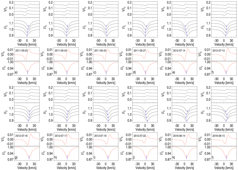
Figure 2: Stokes $V$ (on top) and $I$ (on bottom) LSD profiles for individual subexposures (upper panels) and corresponding final Stokes $V$ and $I$ profiles after having moved the subexposures into the same reference velocity frame (lower panels) for 12 different epochs (a–l). The blue ticks in the Stokes $I$ profiles indicate line centres.

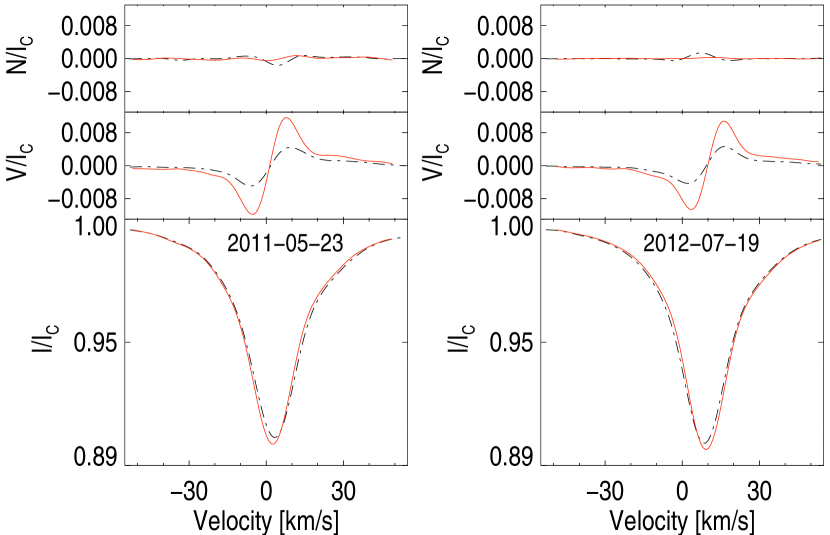
Figure 3: Two examples of Stokes $I$, $V$, and $N$ profile differences for cases where velocity shifts between subexposures have been ignored (black dash-dot line) and where they have been corrected for (red solid line). These plots correspond to subplots (a) and (i) in Fig. 2. The profiles have been calculated using all lines.

Table 2: Longitudinal magnetic field values of HD 96446 computed from HARPSpol data.

HJD	Phase	S/N	$\left<B_{\rm z}\right>_{\rm All}$		$\left<B_{\rm z}\right>_{\rm He}$		$\left<B_{\rm z}\right>_{\rm Si}$		$\left<B_{\rm z}\right>_{\rm metal}$
			(G)		(G)		(G)		(G)
2455704.540	0.13	1133	$-$1189$\pm$	68	$-$1295$\pm$	144	$-$2108$\pm$	256	$-$1075$\pm$	38
2455705.649	0.18	1271	$-$1129$\pm$	39	$-$1216$\pm$	45	$-$2006$\pm$	100	$-$960$\pm$	29
2455706.471	0.22	1713	$-$1113$\pm$	24	$-$1224$\pm$	44	$-$2056$\pm$	80	$-$932$\pm$	17
2455709.457	0.34	1360	$-$896$\pm$	38	$-$1167$\pm$	38	$-$1585$\pm$	141	$-$738$\pm$	21
2456123.477	0.05	1267	$-$1216$\pm$	46	$-$1261$\pm$	46	$-$2213$\pm$	179
2456124.470	0.10	1615	$-$1198$\pm$	21	$-$1247$\pm$	62	$-$2247$\pm$	178
2456125.490	0.14	1300	$-$1142$\pm$	46	$-$1217$\pm$	113	$-$2081$\pm$	71
2456126.481	0.18	1606	$-$1143$\pm$	24	$-$1223$\pm$	28	$-$2015$\pm$	144
2456128.485	0.27	1653	$-$997$\pm$	60	$-$1193$\pm$	23	$-$2034$\pm$	70
2456131.477	0.40	1309	$-$823$\pm$	37	$-$1217$\pm$	10	$-$1584$\pm$	192
2457554.472	0.26	1851	$-$1093$\pm$	47	$-$1224$\pm$	29	$-$2033$\pm$	100
2457555.537	0.30	1871	$-$953$\pm$	51	$-$1211$\pm$	27	$-$1794$\pm$	143

Since He-rich Bp stars usually exhibit surface elemental chemical inhomogeneities, best detectable from the variability of line profiles belonging to the elements He and Si, we also studied the magnetic field strength distribution measured using the samples of He and Si lines separately. A comparison of the Stokes $I$ and $V$ LSD profiles for different samples is presented in Fig. 4. Magnetic field strength values can be found in the literature, i.e., from Borra & Landstreet (1979) and Bohlender et al. (1987), who both used H$\beta$ lines, and from Mathys (1994), whose results are based on selected metallic lines. Similarly, the values obtained by Neiner et al. (2012) are obtained from metal lines and correspond to our first four measurements using the same spectra (see Table 2). The obtained values are in good agreement, taking into account that we have some He lines in our line list.

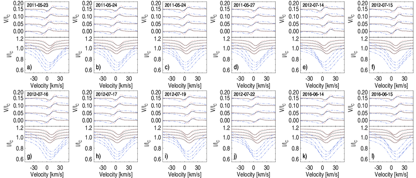
Figure 4: Comparison of Stokes $V$ (top) and $I$ (bottom) LSD profiles for different line masks. The black solid lines are as in Fig. 2 using all 196 lines, the blue dash-dotted lines represent the He line profiles (20 lines), and the red dotted lines are for Si (14 lines).

Due to the presence of surface chemical inhomogeneities in Bp stars, the rotation period of the star can be determined by examining the equivalent width variability of several spectral lines. Based on an extensive time series of high-resolution spectra for HD 96446, Briquet et al. (in preparation) obtained a rotation period of 23.4 d.

Under the assumption of a dipolar magnetic field, the longitudinal magnetic field measurements $\left<B_{\rm z}\right>$ vary as a sine wave. Given our HARPSpol observations over a long time-base, we can refine the value of the rotation frequency $f_{\rm rot}$, performing a non-linear least-squares sine-wave fit to the $\left<B_{\rm z}\right>$-values for all three line lists. From this, we get $f_{\rm rot}=0.04277$ d^-1 for ‘All’. The values obtained when using the magnetic data for the Si lines and for the He lines are fully compatible with the frequency deduced for all lines within 0.00005 d^-1. The corresponding rotation period is $P_{\rm rot}=23.38\pm 0.0273$ d.

In the upper panel of Fig. 5, we present our magnetic field measurements phased with a period of 0.85137 d as suggested by Matthews & Bohlender (1991) and a period of 5.73 d as suggested by Neiner et al. (2012). In the two lower panels, we present the measurements taken from the literature phased with a period of 23.38 d, separately for the measurements using H$\beta$ and for those using metal lines. The corresponding phase diagrams for the mean longitudinal magnetic field measurements using three different line masks, including the best sinusoidal fits, are presented in Fig. 6 where we also show the measurements by Neiner et al. (2012) that were based on selected metallic lines. The increasing trend in field strength between phases 0.1 and 0.4 is also present in the older measurements that were calculated using H$\beta$ (see Fig. 5, lower left-hand panel). The difference between the measurements carried out for the line lists containing He and Si separately shows that the corresponding field strengths are differing at some rotation phases by about 1 kG (see also Columns 5 and 6 in Table 2). The measurements based on the He lines show an almost flat distribution.

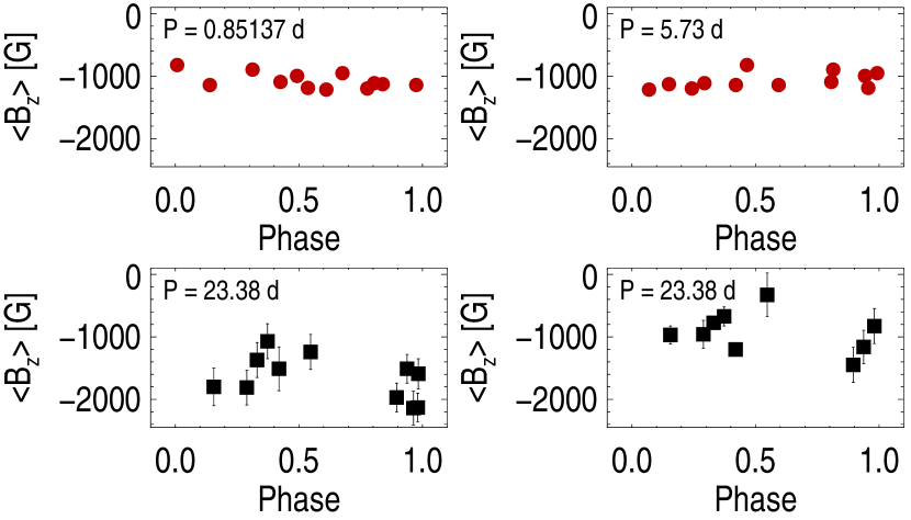
Figure 5: Magnetic field measurement distribution over the rotational phase. On the top panels, red filled circles represent our measurement values that are phased using the two period values as considered in literature and in the lower panels the phases for older literature H$\beta$ (left) and metal (right) values are based on our refined rotation period.

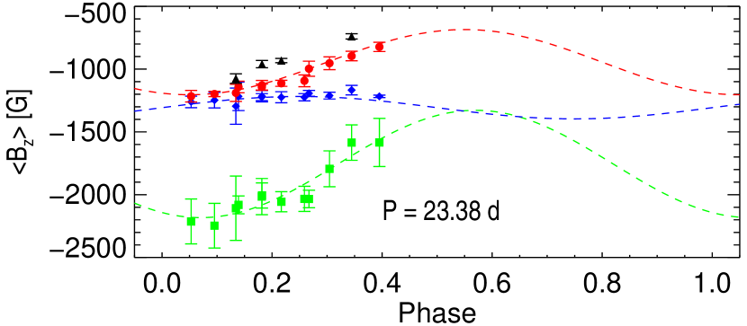
Figure 6: Magnetic field measurement distribution over the rotational phase using the ephemeris $T=2\,455\,000.0+23\aas@@fstack{d}38\ E$. Red filled circles represent values measured from all lines, green squares are from Si lines, and blue diamonds are from He lines. Dashed lines represent the fits. In addition, the values measured by Neiner et al. (2012) using only metal lines are denoted with black triangles.

Assuming that HD 96446 exhibits a single-wave variation of the longitudinal magnetic field during the stellar rotation cycle, we can estimate the parameters of the dipole configuration. Using the oblique rotator model (Stibbs, 1950), $v\sin i=3\pm 2$ km s^-1 and $R=4.45\pm 2.0\,R\odot$ as given by Neiner et al. (2012), and our newly refined rotation period $P_{\rm rot}=23.38\pm 0.0273$ d, we obtain an inclination angle of the stellar rotation axis to the line of sight $i=18\pm 15^{\circ}$ and the equatorial velocity $v_{\rm eq}=10\pm 4$ km s^-1. The variation of the phase curve for the measurements using all lines has a mean of $\overline{\left<B_{\rm z}\right>}=-945\pm 26$ G and an amplitude of $A_{\left<B_{\rm z}\right>}=260\pm 19$ G. From this, we obtain $\left<B_{\rm z}\right>^{\rm min}=-685\pm 32$ G and $\left<B_{\rm z}\right>^{\rm max}=-1205\pm 32$ G. Using the definition by Preston (1967)

$$r=\frac{\left<B_{\rm z}\right>^{\rm min}}{\left<B_{\rm z}\right>^{\rm max}}=\frac{\cos\beta\cos i-\sin\beta\sin i}{\cos\beta\cos i+\sin\beta\sin i},$$ (2)

we find $r=0.568\pm 0.026$ and finally following

$$\beta=\arctan\left[\left(\frac{1-r}{1+r}\right)\cot i\right],$$ (3)

we obtain the magnetic obliquity angle $\beta=40\pm 25^{\circ}$. Assuming the limb-darkening coefficient $u=0.28\pm 0.02$ based on the calculations of Claret & Bloemen (2011) for visual wavelengths and atmospheric parameters of HD 96446 we estimate the dipole strength to be $4.64\pm 0.88$ kG.

As already mentioned in the work of Neiner et al. (2012), the magnetic splitting is best visible in the Fe iii line at 5073.9 Å (Fig. 7). From this magnetically split line, it is possible to determine the mean magnetic field modulus, i.e. the average over the visible stellar hemisphere of the modulus of the magnetic field vector that is weighted by the local line intensity, following the relation given, e.g. by Hubrig & Nesvacil (2007). The observations from 2016 June 14 ($\varphi=0.26$) lead to $\langle|B|\rangle=3.9\pm 0.25$ kG.

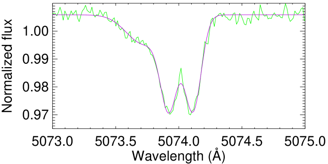
Figure 7: The mean profile of the 2016 June 14 subexposures showing the magnetically split Fe iii line at 5073.9 Å (green) and a triple Gaussian fit to it (purple) to take into account the blend in the blue wing caused by the N ii line at 5073.6 Å.

4 Conclusions

For the analysis of the magnetic field behaviour in the star HD 96446 over the refined rotation period of 23.38 d, we used a sample of archival HARPSpol observations completed by our own most recent observations taken at much higher S/N with the same instrument. We show the strong impact of pulsations on the line profiles and the magnetic field measurements and suggest a specific measurement strategy to account for pulsational variability. For the first time the measurements are carried out for the elements He and Si separately and show that the individual field strengths are differing at some rotation phases by about 1 kG. These elements are usually distributed inhomogeneously over the stellar surface of Bp stars. Model parameters for HD 96446 were constrained assuming a simple magnetic dipole. Compared to the model parameters presented by Neiner et al. (2012), the inclination angle $i$ deduced in our analysis appears to be slightly larger while the value for the magnetic obliquity is in a similar range. While Neiner et al. (2012) estimate the dipole strength between 5 and 10 kG, our modelling results in a much lower value of $4.64\pm 0.88$ kG, which is also consistent with the estimation of the magnetic field modulus of $3.9\pm 0.25$ kG. Due to the relative brightness of HD 96446, the presence of a rather strong magnetic field, and its slow rotation, it can be considered as an excellent target for future high-resolution spectropolarimetric observations over the whole rotation cycle to improve our understanding of the magnetic field structure in massive early B-type stars and the relation between the magnetic structure and the distribution of surface chemical inhomogeneities.

References

- Bohlender et al. (1987) Bohlender D. A., Landstreet J. D., Brown D. N., Thompson I. B., 1987, ApJ, 323, 325
- Borra & Landstreet (1979) Borra E. F., Landstreet J. D., 1979, ApJ, 228, 809
- Claret & Bloemen (2011) Claret A., Bloemen S., 2011, A&A, 529, A75
- Donati et al. (1997) Donati J.-F., Semel M., Carter B. D., Rees D. E., Collier Cameron A., 1997, MNRAS, 291, 658
- Hubrig & Nesvacil (2007) Hubrig S., Nesvacil N., 2007, MNRAS, 378, L16
- Hubrig et al. (2011) Hubrig S., Ilyin I., Briquet M., Schöller M., González J. F., Nuñez N., De Cat P., Morel T., 2011, A&A, 531, L20
- Hubrig et al. (2013) Hubrig S., Ilyin I., Schöller M., Lo Curto G., 2013, Astron. Nachr., 334, 1093
- Kupka et al. (2000) Kupka F. G., Ryabchikova T. A., Piskunov N. E., Stempels H. C., Weiss W. W., 2000, Balt. Astron., 9, 590
- Mathys (1989) Mathys G., 1989, Fundam. Cosm. Phys., 13, 143
- Mathys (1994) Mathys G., 1994, A&AS, 108, 547
- Matthews & Bohlender (1991) Matthews J. M., Bohlender D. A., 1991, A&A, 243, 148
- Neiner et al. (2012) Neiner C., Landstreet J. D., Alecian E., Owocki S., Kochukhov O., Bohlender D., MiMeS Collaboration 2012, A&A, 546, A44
- Preston (1967) Preston G. W., 1967, ApJ, 150, 547
- Ryabchikova et al. (2015) Ryabchikova T., Piskunov N., Kurucz R. L., Stempels H. C., Heiter U., Pakhomov Y., Barklem P. S., 2015, Phys. Scr., 90, 054005
- Snik et al. (2008) Snik F., Jeffers S., Keller C., Piskunov N., Kochukhov O., Valenti J., Johns-Krull C., 2008, in SPIE Conf. Series. p. 22, doi:10.1117/12.787393
- Stibbs (1950) Stibbs D. W. N., 1950, MNRAS, 110, 395