On Hyperbolic graphs induced by
iterated function systems

Abstract.

For any contractive iterated function system (IFS, including the Moran systems), we show that there is a natural hyperbolic graph on the symbolic space, which yields the Hölder equivalence of the hyperbolic boundary and the invariant set of the IFS. This completes the previous studies ([K], [LW1], [W]) by eliminating superfluous conditions, and admits more classes of sets (e.g., the Moran sets). We also show that the bounded degree property of the graph can be used to characterize certain separation properties of the IFS (open set condition, weak separation condition); the bounded degree property is particularly important when we consider random walks on such graphs. This application and the other application to Lipschitz equivalence of self-similar sets will be discussed.

1. Introduction

Let $\{S_{j}\}_{j=1}^{N}$ be a contractive iterated function system (IFS) on ${\mathbb{R}}^{d}$, and let $K$ be the invariant set (attractor) generated by the IFS. It is well-known that the IFS is associated to a finite word space (symbolic space or coding space) $\Sigma^{*}$, which is equipped naturally with a tree structure and a visual metric. The limit set $\Sigma^{\infty}$ of the tree is a Cantor set (topological boundary). Each element of $K$ has a symbolic representation in $\Sigma^{\infty}$, i.e., there is a canonical surjection $\tau:\Sigma^{\infty}\to K$, and $K$ is homeomorphic to the quotient space $\Sigma^{\infty}/\sim$, where the equivalence relation is defined by $\tau(x)=\tau(y)$. In general one would like to impose more information on $\Sigma^{*}$ so as to carry out further analysis on $K$. With the intention to bring in the probabilistic potential theory to $K$, Denker and Sato [DS1,2,3] first constructed a special type of Markov chain $\{Z_{n}\}_{n=0}^{\infty}$ on $\Sigma^{*}$ of the Sierpinski gasket (SG), and showed that the Martin boundary of $\{Z_{n}\}_{n=0}^{\infty}$ is homeomorphic to the SG. Motivated by this, Kaimanovich [K] introduced the concept of “augmented tree” on $\Sigma^{*}$ by adding new edges to the tree $\Sigma^{*}$ according to the intersection of the cells of the IFS, he showed that the graph of the SG is hyperbolic in the sense of Gromov ([G], [Wo]), and that the SG is Hölder equivalent to the hyperbolic boundary of the augmented tree. He also suggested that this approach might also work for other IFS, and the device can be useful to bring in considerations on geometric groups into the study of fractal sets.

The above initiations were carried out by the authors in a series of papers ([JLW], [LW1,2], [W], [DW]). In [LW1], we showed that the hyperbolic boundary and the self-similar set $K$ are Hölder equivalent provided that the IFS satisfies the open set condition (OSC) together with a technical “condition (H)” on $K$ (see Section 2). The Hölder equivalence was used to study the Lipschitz classification of the totally disconnected self-similar sets ([LL], [DLL]), and more generally the Moran sets [L].

In this paper, we unify the previous approaches and obtain the full generality of the Hölder equivalence of the hyperbolic boundaries and the attractors for the general contractive IFS’s. We define the augmented tree on a tree with an associated set-valued map; we also relax the set of augmented edges used previously, so as to remove the OSC on the IFS and the condition (H) on the attractors.

Let $X$ be an infinite set, and let $(X,{\mathcal{E}})$ be a locally finite connected tree. We fixed a reference point $o\in X$ as a root of the tree. For a vertex $x\in X$, we use $|x|$ to denote the length of a non-self-intersecting path from the root to $x$, and let $X_{n}=\{x:|x|=n\}$. Let ${\Sigma}(x)=\{y\in X:\ |y|=|x|+1,\ (x,y)\in{\mathcal{E}}\}$ be the set of offsprings of $x$.

For our purpose, we will denote the edge set of the tree by $\mathcal{E}_{v}$, the set of vertical edges. Let ${\mathcal{K}}$ be the collection of nonempty compact subsets of ${\mathbb{R}}^{d}$. We associate with the tree $(X,\mathcal{E}_{v})$ a set-valued map $\Phi:X\to{\mathcal{K}}$ satisfying

(A1) $\Phi(y)\subset\Phi(x)$ for all $y\in\Sigma(x)$;

(A2)  $\exists$   $\delta_{0}>1$, $0<r<1$  $\ni$  $\delta_{0}^{-1}r^{n}\leq|\Phi(x)|\leq\delta_{0}r^{n}$ for all $x\in X_{n}$, where $|E|$ denotes the diameter of $E$.

Note that for similitudes $\{S_{j}\}_{j=1}^{N}$ with contraction ratio $r$ and self-similar $K$, we can take $X$ to be the symbolic space of finite words, and $\Phi(x)$ to be the cell $S_{x}(K)$ of $K$, then clearly $\Phi$ satisfies (A1), (A2). The reader can refer to Examples 2.1–2.3 for the more general situations about the set-valued map $\Phi$.

Let

$$K_{n}=\bigcup\{\Phi(x):\ x\in X_{n}\}\quad\mbox{and}\quad K=\bigcap_{n=0}^{\infty}K_{n}.$$ (1.1)

By (A1), $\{K_{n}\}_{n=1}^{\infty}$ is a decreasing sequence of compact sets. Hence $K\in{\mathcal{K}}$ is a nonempty compact set of ${\mathbb{R}}^{d}$, we call $K$ the attractor of $\Phi$. We use the map $\Phi$ to induce another set of edges called a horizontal edges set: for a fixed $\kappa>0$, define

$${\mathcal{E}}_{h}:=\{(x,y)\in X\times X:|x|=|y|,\ x\not=y,\ {\rm dist}(\Phi(x),\Phi(y))\leq\kappa r^{|x|}\}.$$ (1.2)

Definition 1.1.

(Augmented tree) Let $(X,{\mathcal{E}}_{v})$ be a tree and ${\mathcal{E}}_{h}$ be defined as (1.2), and let ${\mathcal{E}}={\mathcal{E}}_{v}\cup{\mathcal{E}}_{h}$, we call the graph $(X,{\mathcal{E}})$ an augmented tree.

For a contractive IFS $\{S_{j}\}_{j=1}^{N}$ with an attractor $K$, it is easy to see that a tree $(X,{\mathcal{E}}_{v})$ and a set-valued map $\Phi$ arise naturally from the symbolic space, and the augmented tree can be defined (Example 2.1). More generally, the Moran construction of the Moran sets ([M], [FWW]) which admits a more flexible iterated scheme, can also be fitted into the above framework (Example 2.2). On the other hand, for any compact set $K\subset{\mathbb{R}}^{d}$, we can construct a tree and the above map $\Phi$ such that the augment tree so defined has $K$ as the attractor (Example 2.3).

Remark. We point out that the main departure of the augmented tree in Definition 1.1 from the one in [K] and [LW1] is the modification of the ${\mathcal{E}}_{h}$ in (1.2); over there the horizontal edge was defined by a more restrictive condition $\Phi(x)\cap\Phi(y)\not=\emptyset$ (i.e., $\kappa=0$). As the intersection of the cells can be very delicate, the new definition adds in more edges to bypass the dependence of the fine structure of the intersection in the intermediary levels, but preserves the structure at infinity (the specific $\kappa>0$ is not important). It allows us to remove the superfluous conditions in the previous studies.

Our first main theorem is

Theorem 1.2.

Assume that the mapping $\Phi:\ X\longrightarrow{\mathcal{K}}$ satisfying (A1) and (A2), then the augmented tree $(X,{\mathcal{E}})$ in Definition 1.1 is a hyperbolic graph in the sense of Gromov (see Definition 2.8).

It follows from the hyperbolicity that the augmented tree $(X,{\mathcal{E}})$ admits a “visual metric” $\rho_{a}(\cdot,\cdot)$ defined by the Gromov product (see Definition 2.7), which is extended to the completion $\widehat{X}$ of $X$. The hyperbolic boundary is defined as $\partial X=\widehat{X}\setminus X$. Our next main theorem is

Theorem 1.3.

With the same assumptions as in Theorem 1.2, the hyperbolic boundary $\partial X$ of $(X,{\mathcal{E}})$ is Hölder equivalent to the attractor $K$ in (1.1) , i.e., there exists a natural bijection $\iota:\ \partial X\longrightarrow K$ and a constant $C>0$ such that

$$C^{-1}|\iota(\xi)-\iota(\eta)|\leq\rho_{a}^{\beta}(\xi,\eta)\leq C|\iota(\xi)-\iota(\eta)|,\quad\forall\ \xi,\eta\in\partial X,$$ (1.3)

with $\beta=-(\log r)/{a}$.

Recall that a graph $(X,{\mathcal{E}})$ is of bounded degree if $\max\{{\rm deg}(x):x\in X\}<\infty$, where ${\rm deg}(x)=\#\{y\in X:\ (x,y)\in{\mathcal{E}}\}$ is the total number of edges joining $x$. Bounded degree is an important property, especially when we study random walks on graphs. The following two theorems are for IFS of contractive similitudes.

Theorem 1.4.

Let $(X,{\mathcal{E}})$ be the augmented tree induced by an IFS of contractive similitudes. Then $(X,{\mathcal{E}})$ is of bounded degree if and only if $\{S_{j}\}_{j=1}^{N}$ satisfies the OSC.

For an IFS that does not satisfy the OSC, it may happen that $S_{x}=S_{y}$ for $x\not=y$. We can modify the augmented tree $(X,{\mathcal{E}})$ of $\{S_{j}\}_{j=1}^{N}$ by identifying $x,y\in X$ for $|x|=|y|$ and $S_{x}=S_{y}$, and let $(X^{\sim},\mathcal{E})$ denote the quotient space with the induced graph, then following the same proof, it is seen that Theorems 1.2, 1.3 still hold for $(X^{\sim},{\mathcal{E}})$. Moreover we have

Theorem 1.5.

The graph $(X^{\sim},{\mathcal{E}})$ is of bounded degree if and only if the IFS satisfies the weak separation condition.

The definition of the weak separation condition (WSC) will be recalled in Section 4. It includes IFS with overlaps, and has been studied in detail in connection with the multifractal structure of self-similar measures (see [LN], [FL], [DLN] and the references therein).

The Hölder equivalence of the self-similar sets and the hyperbolic boundaries in Theorem 1.3 is very useful. As an illustration, we will give a brief discussion of two such applications in Section 5. The first one is on the Lipschitz equivalence of totally disconnected self-similar sets, which relies on a “near-isometry” of the augmented trees ([LL], [DLL]); the second one concerns the Martin boundaries of certain random walks on the augmented trees [KLW] and the induced Dirichlet forms, in which the graph with bounded degree will play an important role.

For the organization of the paper, we will state some basic facts on hyperbolic graphs and include a few important examples of augmented tree in Section 2. We prove Theorems 1.2, 1.3 in Section 3. In Section 4, the OSC and WSC will be recalled, and Theorem 1.4, 1.5 will be proved. In Section 5, we include two significant applications of Theorem 1.3 described in the last paragraph. Finally, we will discuss some other variations of the augmented trees in Section 6.

2. Augmented trees and hyperbolic graphs

In this section, we first recall some basic notations for a graph. Let $X$ be a countable set, a (undirected simple) graph is a pair $(X,{\mathcal{E}})$, where ${\mathcal{E}}$ is a symmetric subset of $X\times X\setminus\{(x,x):\ x\in X\}$. We call $x\in X$ a vertex and $(x,y)\in{\mathcal{E}}$ an edge, also denote by $x\sim y$. The degree of a vertex $x$ is the total number of edges which connect to $x$ and is denoted by ${\rm deg}(x)$, the graph is locally finite if ${\rm deg}(x)<\infty$ for all $x\in X$. For $x,y\in X\ (x\not=y)$, a path from $x$ to $y$ is a finite sequence $\{x_{0},x_{1},\cdots,x_{n}\}$ such that $x_{0}=x,\ x_{n}=y$ and $(x_{i},x_{i+1})\in{\mathcal{E}}$, and is denoted by $p(x_{0},x_{1},\cdots,x_{n})$. Moreover, if the above path $p(x_{0},x_{1},\cdots,x_{n})$ has the minimal length among all possible paths from $x$ to $y$, then we say that the path is a geodesic and denote by $\pi(x_{0},x_{1},\cdots,x_{n})$. Denote $d(x,y)$ the length of a geodesic from $x$ to $y$, then $d(x,y)$ is an integer-valued metric on $X$. Throughout the paper, we assume that the graph is locally finite and connected, i.e., any two different vertices can be connected by a path.

A graph is called a tree if any two vertices can be connected by a unique non-self-intersecting path. We fix a reference point $o\in X$ and call it the root of the tree, denote by $|x|=d(o,x)$ the distance from the root to the vertex $x$. For a tree $(X,{\mathcal{E}}_{v})$ and $x\in X\setminus\{o\}$, we let $x^{-1}$, the parent of $x$, be the unique vertex such that $(x^{-1},x)\in{\mathcal{E}}_{v}$ and $|x^{-1}|=|x|-1$. Inductively, we define $x^{-k}=(x^{-(k-1)})^{-1}$ to be the $k$-th generation ancestor of $x$. Let $\Sigma(x)=\{y\in X:\ y^{-1}=x\}$ be the set of the offsprings of $x$.

We first give some examples of the augmented tree $(X,\mathcal{E})$ in Definition 1.1.

Example 2.1.

Let $\{S_{j}\}_{j=1}^{N}$ be a contractive IFS on ${\mathbb{R}}^{d}$. It is well-known that there exists a nonempty compact subset $K\subset{\mathbb{R}}^{d}$ such that $K=\bigcup_{j=1}^{N}S_{j}(K)$. We call the set $K$ the invariant set of the IFS, and a self-similar set if $\{S_{j}\}_{j=1}^{N}$ are contractive similitudes.

Let $\Sigma^{*}=\bigcup_{n=0}^{\infty}\{1,2,\cdots,N\}^{n}$. For each $x=i_{1}i_{2}\cdots i_{n}\in\Sigma^{*}$, denote $S_{x}=S_{i_{1}}\circ S_{i_{2}}\circ\cdots\circ S_{i_{n}}$ the composition, and $K_{x}=S_{x}(K)$. Let

$$r_{x}=\inf\{\frac{|S_{x}(a)-S_{x}(b)|}{|a-b|}:\ a,b\in{\mathbb{R}}^{d},\ a\not=b\},$$

and

$$R_{x}=\sup\{\frac{|S_{x}(a)-S_{x}(b)|}{|a-b|}:\ a,b\in{\mathbb{R}}^{d},\ a\not=b\},$$

be the minimal and maximal contractions of the map $S_{x}(\cdot)$. Let $r=\min\{r_{1},r_{2},\cdots,r_{N}\}>0$ and $R=\max\{R_{1},R_{2},\cdots,R_{N}\}<1$, we define a new coding space

$${\mathcal{J}}_{n}=\{i_{1}i_{2}\cdots i_{k}\in\Sigma^{*}:\ R_{i_{1}i_{2}\cdots i_{k}}\leq r^{n}<R_{i_{1}i_{2}\cdots i_{k-1}}\}\quad\mbox{and}\quad X=\bigcup_{n=0}^{\infty}{\mathcal{J}}_{n}.$$

Then each $S_{x}(K):=K_{x},\ x\in{\mathcal{J}}_{n}$ has diameter of order $r^{n}$. There is a natural tree structure on $X$ as following: for $x=i_{1}i_{2}\cdots i_{k}\in{\mathcal{J}}_{n}$ ($n>0$), let $x^{-1}=i_{1}i_{2}\cdots i_{\ell}$ ($\ell<k$) be the initial part of $x$ such that $x^{-1}\in{\mathcal{J}}_{n-1}$. Define

$${\mathcal{E}}_{v}=\{(x,x^{-1}),(x^{-1},x):\ x\in X\setminus\{\vartheta\}\},$$ (2.1)

where $\vartheta$ is the empty word. Then $(X,{\mathcal{E}}_{v})$ is a tree with root $o=\vartheta$. Furthermore, we define the map $\Phi:\ X\longrightarrow{\mathcal{K}}$ as $\Phi(x)=K_{x}$. Then the map $\Phi(\cdot)$ satisfies (A1) and (A2). Moreover, the invariant set $K$ of the IFS coincides with the one in (1.1).

For the special case that the IFS $\{S_{j}\}_{j=1}^{N}$ on ${\mathbb{R}}^{d}$ are contractive similitudes , we have $r_{x}=R_{x}$, and hence

$${\mathcal{J}}_{n}=\{i_{1}i_{2}\cdots i_{k}\in\Sigma^{*}:\ r_{i_{1}i_{2}\cdots i_{k}}\leq r^{n}<r_{i_{1}i_{2}\cdots i_{k-1}}\},$$

where $r=\min\{r_{i}:\ i=1,2,\cdots,N\}$ is the minimal contraction ratio of the $\{S_{j}\}_{j=1}^{N}$. The augmented tree of this class of IFS was studied in detail in [LW1] and [W], where the horizontal edge set is defined by the more restrictive condition: $\Phi(x)\cap\Phi(y)=K_{x}\cap K_{y}\not=\emptyset$.    $\Box$

Example 2.2.

A Moran set is a generalization of a self-similar set with a more general coding space ([M], [FWW], [L]). Given a tree $X=\bigcup_{n=0}^{\infty}X_{n}$ with root $\vartheta$, a compact set $J$ with nonempty interior, and a sequence of $\{r_{k}\}_{n=1}^{\infty},0<r_{k}<1$, it is associated with a family of compact sets with nonempty interior $\{J_{x}:x\in X\}$ such that

(i) $J_{\vartheta}=J$, and for any $x\in X$, $J_{x}$ is geometrically similar to $J$;

(ii) for $x\in X_{n},\ y\in\Sigma(x)$, $J_{y}\subset J_{x}$,  and $J^{o}_{y}\cap J^{o}_{y^{\prime}}=\emptyset$ for $y\not=y^{\prime}$ in $\Sigma(x)$;

(iii) for $x\in X_{n},\ y\in\Sigma(x)$, $\frac{|J_{y}|}{|Jx|}=r_{n}$.

The Moran set is defined to be $K=\bigcap_{n\geq 0}\bigcup_{x\in X_{n}}J_{x}$.

It is clear that the map $\Phi(x)=J_{x}$ satisfies (A1), but not necessarily (A2). To handle this, we assume that $\inf\{r_{n}:\ n=1,2,\cdots\}:=r>0$ and construct a new tree $(Y,{\mathcal{E}}^{M})$ as follow: Let $Y_{0}=X_{0}$. For each integer $k>0$, denote by $n(k)$ the integer such that $r_{1}r_{2}\cdots r_{n(k)}\leq r^{k}<r_{1}r_{2}\cdots r_{n(k)-1}$ (same idea as in last example). Let $Y_{k}=X_{n(k)}$ and $Y=\bigcup_{k=0}^{\infty}Y_{k}$. Then $Y$ is a subset of $X$, define the edge set ${\mathcal{E}}_{v}$ on $Y$ in the obvious way: for $y_{1}\in Y_{k-1}$, $y_{2}\in Y_{k}$, $(y_{1},y_{2})\in{\mathcal{E}}_{v}$ if there is a geodesic path with length $n(k)-n(k-1)$ in the tree $(X,{\mathcal{E}})$. We get a new tree $(Y,{\mathcal{E}}_{v})$. Then the set-valued map $\Phi(y)=J_{y}$ on $Y$ satisfies (A1) and (A2). Moreover, the Moran set $K$ satisfies (1.1).   $\Box$

Our next example shows that we can associate an augmented tree structure to any compact set in ${\mathbb{R}}^{d}$.

Example 2.3.

Let $K$ be a nonempty compact subset in ${\mathbb{R}}^{d}$. Then there is a tree $(X,\mathcal{E}_{v})$ and a set-valued map $\Phi$ which generate an augmented tree $(X,\mathcal{E})$ such that the compact subset $K$ satisfies (1.1).

Without loss of generality, we assume that $K\subset[0,1]^{d}$. Let ${\mathcal{F}}_{k},k\geq 0$ be the dyadic partitions of $[0,1]^{d}$ into subcubes of size $2^{-k}$. Note that $\mathcal{F}_{k+1}$ is a refinement of $\mathcal{F}_{k}$. Let $x_{0,1}=[0,1]^{d}$ and $X_{0}=\{x_{0,1}\}$. Suppose we have chosen $X_{k}=\{x_{k,1},\cdots,x_{k,n_{k}}\}$ as the family of dyadic subcubes in ${\mathcal{F}}_{k}$ that intersects $K$. Choose $X_{k+1}$ to be the dyadic subcubes of $x_{k,i}$ in ${\mathcal{F}}_{k+1}$ that intersects $K$. In this way we obtain a refining sequence $\{X_{n}\}_{n=0}^{\infty}$ of families of subcubes. Letting $X=\bigcup_{n=0}^{\infty}X_{n}$ and considering these subcubes as a vertex of $X$, there is a natural tree structure $\mathcal{E}_{v}$ on $X$ connecting $x_{k,i}$ and its offsprings. Letting $\Phi:X\to{\mathcal{K}}$ be such that $\Phi(x)$ is the subcube $x$, $\Phi$ satisfies (A1) and (A2). The augmented tree can be constructed accordingly.   $\Box$

In additional to the notion of augmented tree defined in Section 1, we introduce another more general concept.

Definition 2.4.

(Pre-augmented tree) We call a graph $(X,\mathcal{E})$ a pre-augmented tree if $\mathcal{E}=\mathcal{E}_{v}\cup\mathcal{E}_{h}$ where

(i) $(x,y)\in\mathcal{E}_{h}$ implies $|x|=|y|$; and

(ii) $(x,y)\in{\mathcal{E}}_{h}$ implies either $x^{-1}=y^{-1}$ or $(x^{-1},y^{-1})\in{\mathcal{E}}_{h}$.

Remark 2.5.

The pre-augmented tree is a rather flexible device to study the hyperbolicity of the graphs (Proposition 2.9). The following proposition shows that augmented tree is pre-augmented tree. On the other hand, it is easy to find a pre-augmented tree that is not an augmented tree (see Section 6 for the simple construction of a discrete hyperbolic disc).

Proposition 2.6.

An augmented tree $(X,{\mathcal{E}})$ is a pre-augmented tree.

Proof. The proposition follows from the following simple observation: $\Phi(x)\subset\Phi(x^{-1}),\ \Phi(y)\subset\Phi(y^{-1})$ (by assumption (A1)), hence for $(x,y)\in{\mathcal{E}}_{h}$,

$${\rm dist}\big{(}\Phi(x^{-1}),\Phi(y^{-1})\big{)}\leq{\rm dist}\big{(}\Phi(x),\Phi(y)\big{)}\leq\kappa r^{|x|}<\kappa r^{|x^{-1}|},$$

so that either $x^{-1}=y^{-1}$ or $(x^{-1},y^{-1})\in{\mathcal{E}}_{h}$. $\Box$

For the edge set ${\mathcal{E}}={\mathcal{E}}_{v}\cup{\mathcal{E}}_{h}$ in a pre-augmented tree, a path is call a vertical (horizontal) path if it consists of only vertical (horizontal, respectively) edges. A vertical path is always a geodesic if it is not self-intersect; we call a path horizontal geodesic if it is a horizontal path and is a geodesic in ${\mathcal{E}}$. A geodesic from $x$ to $y$ is not unique in general, but it can be reduced to the following expression

$$\pi(x,x^{-1},\cdots,x^{-k})\cup\pi(x^{-k},z_{1},\cdots,z_{\ell},y^{-k^{\prime}})\cup\pi(y^{-k^{\prime}},\cdots,y^{-1},y),$$ (2.2)

where the first and last part are vertical geodesics, and the middle part is a horizontal geodesic in $X_{n}:=\{x\in X:\ |x|=n\}$ for some $n$ (it is possible that one or two parts may vanish) ([K], [LW1]). We call it a canonical geodesic if the $n$ is the smallest (i.e., $X_{n}$ is at the highest level) among such expression (see Figure 1).

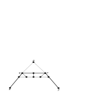
Figure 1. Canonical geodesic

Definition 2.7.

Let $(Y,{\mathcal{G}})$ be a graph, for $x,y\in Y$, we call the quantity

$$|x\wedge y|:=\frac{1}{2}(|x|+|y|-d(x,y)),\quad\forall\ x,\ y\in Y,$$

the Gromov product of $x$ and $y$ (with respect to a root $o$).

Definition 2.8.

A graph $(Y,{\mathcal{G}})$ is called hyperbolic if there exists a constant $\delta>0$ such that

$$|x\wedge y|\geq\min\{|x\wedge z|,\ |z\wedge y|\}-\delta,\quad\forall\ x,\ y,\ z\in Y.$$

The reader can refer to [Wo] for various equivalent definitions of hyperbolic graphs, in particular, for the geometric definition that every geodesic triangle is “$\delta$-thin”. Note that for the augmented tree $(X,\mathcal{E})$, and for a canonical geodesic in (2.2), we can express the Gromov product as [LW1]

$$|x\wedge y|=n-(\ell+1)/2,$$ (2.3)

where $n$ and $(\ell+1)$ are the level and the length of the horizontal part of the canonical geodesic in (2.2) respectively.

Theorem 2.9.

[LW1, Theorem 2.3] A pre-augmented tree $(X,\mathcal{E})$ is hyperbolic if and only if there exists a constant $L>0$ such that the lengths of all horizontal geodesics are bounded by $L$.

3. Proof of Theorem 1.2 and Theorem 1.3

We will make use of the special form of geodesic in an augmented tree and Theorem 2.9 to prove the two main theorems.

Proof of Theorem 1.2.   Let $(X,\mathcal{E})$ be an augmented tree with the associated set-valued map satisfies (A1) and (A2). Suppose $(X,{\mathcal{E}})$ is not hyperbolic, then by Theorem 2.9, for any integer $m>0$, there exists a horizontal geodesic $\pi(x_{0},x_{1},\cdots,x_{3m})$ (length $3m$) in some level $n$, i.e., $|x_{i}|=d(o,x_{i})=n$. Note that $p(x_{0},x_{0}^{-1},\cdots,o,\cdots,x_{3m}^{-1},x_{3m})$ is a path joining $x_{0}$ and $x_{3m}$, it follows that $2n\geq 3m$. Hence $n>m$. We consider the set $\{x_{0}^{-m},x_{1}^{-m},\cdots,x_{3m}^{-m}\}$, the $m$-th generation ancestor of $\pi(x_{0},x_{1},\cdots,x_{3m})$. The property of augmented tree (Proposition 2.6) implies that either $x_{i}^{-m}=x_{i+1}^{-m}$ or $(x_{i}^{-m},x_{i+1}^{-m})\in{\mathcal{E}}_{h}$. Hence there is a path $p(y_{0},y_{1},\cdots,y_{\ell})$ joining $x_{0}^{-m}$ and $x_{3m}^{-m}$, where $y_{0}=x_{0}^{-m},\ y_{\ell}=x_{3m}^{-m}$ and $y_{i}\in\{x_{0}^{-m},x_{1}^{-m},\cdots,x_{3m}^{-m}\},\ i=0,1,\cdots,\ell$. We assume without loss of generality that the above path $p(y_{0},y_{1},\cdots,y_{\ell})$ has the minimal length among all possible horizontal paths joining $x_{0}^{-m}$ and $x_{3m}^{-m}$. Now we get a new path

$$\pi(x_{0},x_{0}^{-1},\cdots,x_{0}^{-m})\cup p(y_{0},y_{1},\cdots,y_{\ell})\cup\pi(x_{3m}^{-m},\cdots,x_{3m}^{-1},x_{3m})$$

joining $x_{0}$ and $x_{3m}$ (see Figure 2). Note that $\pi(x_{0},x_{1},\cdots,x_{3m})$ is a geodesic path, hence has minimal length. By comparing the lengths of the two paths, we have $\ell\geq m$.

Figure 2. The two paths joining $x_{0}$ and $x_{3m}$.

Let

$$D=\bigcup_{i=0}^{3m}\Phi(x_{i})\quad\mbox{and}\quad D^{\prime}=\bigcup_{i=0}^{\ell}\Phi(y_{i}).$$

We estimate the diameter of $D$ and $D^{\prime}$ as follows. By (A2) and (1.2), we have $|\Phi(x_{i})|\leq\delta_{0}r^{n}$ and ${\rm dist}(\Phi(x_{i}),\Phi(x_{i+1}))\leq\kappa r^{n}$. Hence

$$|D|\leq\sum_{i=0}^{3m-1}\big{(}|\Phi(x_{i})|+{\rm dist}(\Phi(x_{i}),\Phi(x_{i+1}))\big{)}+|\Phi(x_{3m})|<(3m+1)(\delta_{0}+\kappa)r^{n}.$$

For each $i$, there exists $j$ such that $y_{i}=x_{j}^{-m}$. It follows that $\Phi(x_{j})\subset\Phi(y_{i})$. Hence $\Phi(y_{i})\cap D\not=\emptyset$. This yields

$$|D^{\prime}|\leq 2\max_{i}\{|\Phi(y_{i})|\}+|D|\leq 2\delta_{0}r^{n-m}+(3m+1)(\delta_{0}+\kappa)r^{n}.$$

We take $m$ large enough such that $(3m+1)(\delta_{0}+\kappa)r^{m}<\delta_{0}$. Then $|D^{\prime}|<3\delta_{0}r^{n-m}$. (This is the key step to use $D^{\prime}$ so as to absorb the factor $(3m+1)$ in the estimation of $|D|$.) Hence there is a ball $B$ with radius $3\delta_{0}$ such that

$$r^{m-n}D^{\prime}=\bigcup_{i=0}^{\ell}r^{m-n}\Phi(y_{i})\subset B.$$

On the other hand, let $a_{i}\in r^{m-n}\Phi(y_{i})$, and let $\ell^{\prime}=[\ell/2]$, the largest integer $\leq\ell/2$, we claim that the distances of any two points in the set $\{a_{0},a_{2},\cdots,a_{2\ell^{\prime}}\}$ of even indices are at least $\kappa(>0)$. Indeed, by assumption, $p(y_{0},y_{1},\cdots,y_{\ell})$ is a horizontal path from $y_{0}$ to $y_{\ell}$ with minimal length. Hence $(y_{i},y_{j})\not\in{\mathcal{E}}_{h}$ for any $j\geq i+2$ (otherwise, $p(y_{0},\cdots,y_{i},y_{j},\cdots,y_{\ell})$ is also a path, but has a shorter length). By the definition of horizontal edge in (1.2), we have ${\rm dist}(\Phi(y_{i}),\Phi(y_{j}))>\kappa r^{(n-m)}$. Hence $|a_{i}-a_{j}|\geq{\rm dist}(r^{m-n}\Phi(y_{i}),r^{m-n}\Phi(y_{j}))\geq\kappa$, and the claim follows.

The claim implies that the ball $B$ contains at least $\ell^{\prime}+1>m/2$ points $a_{0},a_{2},\cdots,a_{2\ell^{\prime}}$ such that any two of them are separated by a distance at least $\kappa(>0)$. Since $m$ can arbitrarily large, this is impossible, and completes the proof of the theorem. $\Box$

For $a>0$ small (say, $e^{3\delta a}<\sqrt{2}$ [Wo]), let

$$\rho_{a}(x,y)=\exp(-a|x\wedge y|),\ \quad\forall\ x,y\in X,\ x\not=y,$$ (3.1)

and $\rho_{a}(x,x)=0$. Then $\rho_{a}(\cdot,\cdot)$ satisfies

$$\rho_{a}(x,y)\leq C\max\{\rho_{a}(x,z),\ \rho_{a}(z,y)\},\quad\forall\ x,y,z\in X,$$ (3.2)

for some constant $C\geq 1$. It is known that $\rho_{a}(\cdot,\cdot)$ is not a metric (unless $C=1)$, but is equivalent to a metric; we can hence regard $\rho_{a}(\cdot,\cdot)$ as a metric for convenience. By definition (3.1), it is clear that for a sequence $\{x_{n}\}_{n=0}^{\infty}\subset X$ with $\lim_{n\to\infty}|x_{n}|=\infty$, then $\{x_{n}\}_{n=0}^{\infty}$ is a $\rho_{a}$-Cauchy sequence if and only if $|x_{n}\wedge x_{m}|\to\infty$ as $m,\ n\to\infty$.

Definition 3.1.

Let $\widehat{X}$ be the $\rho_{a}$-completion of $X$, it is a compact set. We call $\partial X=\widehat{X}\setminus X$ to be the hyperbolic boundary of $X$.

Definition 3.2.

A sequence $\{x_{n}\}_{n=0}^{\infty}\subset X$ is called a geodesic ray and denoted by $\pi(x_{0},x_{1},\cdots)$, if $x_{0}=o$, $|x_{n}|=n$ and $(x_{n},x_{n+1})\in{\mathcal{E}}_{v}$.

A geodesic ray is a shortest path from the root $o$ to infinity. It is useful to identify $\xi\in\partial X$ with equivalent geodesic rays that converge to $\xi$. Also it is known [Wo] that two geodesic rays $\pi(x_{0},x_{1},\cdots)$ and $\pi(y_{0},y_{1},\cdots)$ are equivalent as $\rho_{a}$-Cauchy sequences if and only if there is $c>0$ such that

$$d(x_{n},y_{n})\leq c$$ (3.3)

for all but finitely $n$, where $c$ depends only on the $\delta$ in Definition 2.8 of hyperbolic graph (The constant $c$ can be taken to be $1$ here, see the following Proof of Theorem 1.3, the part on $\iota$ is injective). Moreover, the Gromov product and $\rho_{a}(\cdot,\cdot)$ can be extended to $X\cup\partial X$ by letting

$$|x\wedge\xi|=\inf\{\lim_{n\to\infty}|x\wedge x_{n}|\},\ \quad|\xi\wedge\eta|=\inf\{\lim_{n\to\infty}|x_{n}\wedge y_{n}|\},$$ (3.4)

where $x\in X$, $\xi,\eta\in\partial X$, and the infimum is taking over all geodesic rays $\pi(x_{0},x_{1},\cdots)$ and $\pi(y_{0},y_{1},\cdots)$ converging to $\xi$ and $\eta$ respectively. The metric on $X\cup\partial X$ is defined in the same way as in (3.1), and inequality (3.2) still holds on $X\cup\partial X$.

Proof of Theorem 1.3.  For $\xi\in\partial X$, we let $\pi(x_{0},x_{1},\cdots)$ be a geodesic ray representing $\xi$. Then the sequence of compact sets $\{\Phi(x_{n})\}_{n}$ is decreasing on $n$ and $|\Phi(x_{n})|\to 0$ as $n\to\infty$. Hence the intersection $\bigcap_{n=0}^{\infty}\Phi(x_{n})$ is a singleton. We define $\iota:\ \partial X\longrightarrow K$ by

$$\{\iota(\xi)\}=\bigcap_{n=0}^{\infty}\Phi(x_{n}).$$

We first show that $\iota$ is well defined. Let $\pi(y_{0},y_{1},\cdots)$ be a geodesic ray which is equivalent to $\pi(x_{0},x_{1},\cdots)$. Assume that $\bigcap_{n=0}^{\infty}\Phi(x_{n})=\{a_{x}\}$ and $\bigcap_{n=0}^{\infty}\Phi(y_{n})=\{a_{y}\}$, we need to show that $a_{x}=a_{y}$. Indeed, for each $n$, let

$$\pi(x_{n},x_{n-1},\cdots,x_{n-\ell})\cup\pi(x_{n-\ell},z_{1},\cdots,z_{k},y_{n-\ell})\cup\pi(y_{n-\ell},\cdots,y_{n-1},y_{n})$$

be a canonical geodesic joining $x_{n}$ and $y_{n}$. Then

$$a_{x}\in\Phi(x_{n})\subset\Phi(x_{n-\ell}),\quad a_{y}\in\Phi(y_{n})\subset\Phi(y_{n-\ell}).$$

Therefore

$$|a_{x}-a_{y}| \leq|\Phi(x_{n-\ell})|+\kappa r^{n-\ell}+\sum_{i=1}^{k}\Big{(}|\Phi(z_{i})|+\kappa r^{n-\ell}\Big{)}+|\Phi(y_{n-\ell})|$$

$$<(k+2)(\delta_{0}+\kappa)r^{n-\ell}.$$

On the other hand, (3.3) implies that $d(x_{n},y_{n})=2\ell+(k+1)\leq c$ for some constant $c>0$. We conclude that $|a_{x}-a_{y}|\leq C^{\prime}r^{n}$ for some $C^{\prime}>0$ and $n$ large enough. It follows that $a_{x}=a_{y}$, and the map $\iota$ is well defined.

Next we show that $\iota$ is surjective. As for any $a_{0}\in K$, there exists $\{x_{n}\}\subset X$ with $|x_{n}|=n$ such that $a_{0}\in\Phi(x_{n})$ for all integer $n\geq 0$ (this $\{x_{n}\}_{n}$ may not be a geodesic ray). As $X_{n}=\{x\in X:\ |x|=n\}$ is a finite set for all $n$, there exists $y_{1}\in X_{1}$ and infinite many $\{x_{n_{11}},x_{n_{12}},\cdots\}\subset\{x_{n}\}_{n}$ such that they are all descendents of $y_{1}$. Assume that we have defined the sequence $\{x_{n_{k1}},x_{n_{k2}},\cdots\}$ and $y_{k}\in X_{k}$ such that $\{x_{n_{k1}},x_{n_{k2}},\cdots\}$ are all descendants of $y_{k}\in X_{k}$. Since $\Sigma(y_{k})<\infty$, we know that there exist $y_{k+1}\in\Sigma(y_{k})$ and a subsequence $\{x_{n_{(k+1)1}},x_{n_{(k+1)2}},\cdots\}$ of $\{x_{n_{k1}},x_{n_{k2}},\cdots\}$ such that they are all offspring of $y_{k+1}$. It is clear that $\{y_{0},y_{1},y_{2},\cdots\}$ is a geodesic ray. Since this geodesic ray will converge to some point $\xi\in\partial X$, it follows that $\{\iota(\xi)\}=\bigcap_{k=0}^{\infty}\Phi(y_{k})=\{a_{0}\}$. This completes the proof that $\iota$ is surjective.

To show that $\iota$ is injective, we assume that $\xi,\ \eta\in\partial X$ and $\iota(\xi)=\iota(\eta)$. We claim that $\xi=\eta$. For this, let $\pi(x_{0},x_{1},\cdots)$ and $\pi(y_{0},y_{1},\cdots)$ be geodesic rays converging to $\xi$ and $\eta$ respectively. Let $a_{0}=\iota(\xi)=\iota(\eta)$, then $a_{0}\in\Phi(x_{n})\cap\Phi(y_{n})$ for all $n$. It implies that either $x_{n}=y_{n}$ or $(x_{n},y_{n})\in{\mathcal{E}}_{h}$. Hence $d(x_{n},y_{n})\leq 1$ for all integer $n$. We therefore conclude that the two geodesic rays are equivalent, i.e., $\xi=\eta$.

Finally, we show that $\iota$ is a Hölder equivalence mapping. If $\xi=\eta$, then (1.3) is trivial, hence we assume that $\xi\not=\eta$ in the following. Let $\pi(x_{0},x_{1},\cdots)$ and $\pi(y_{0},y_{1},\cdots)$ be geodesic rays converging to $\xi$ and $\eta$ respectively, and moreover, they attain the infimum in (3.4). There is a bilateral canonical geodesic $\pi(\cdots,x_{k+1},x_{k})\cup\pi(x_{k},z_{1},\cdots,z_{\ell},y_{k})\cup\pi(y_{k},y_{k+1},\cdots)$ joining $\xi$ and $\eta$, where the first and the third parts are vertical paths, and the middle part is a horizontal geodesic. Then $|x_{n}\wedge y_{n}|=k-(\ell+1)/2$ for all $n\geq k$ (see (2.3)), and

$$\rho_{a}(\xi,\eta)=\exp(-a|\xi\wedge\eta|)=\exp\{-a(k-\frac{1}{2}(\ell+1))\}.$$

By making use of Theorem 2.9, we see that the length of the horizontal geodesic $\pi(x_{k},z_{1},\cdots,z_{\ell},y_{k})$ is bounded by the constant $L$. This implies that there exists $C_{1}>0$ such that

$$C_{1}^{-1}\exp(-ak)\leq\rho_{a}(\xi,\eta)\leq C_{1}\exp(-ak).$$

To prove the lower bound of the inequality in (1.3), we observe that

$$\iota(\xi)\in\Phi(x_{n+k})\subset\Phi(x_{k})\quad\mbox{and}\quad\iota(\eta)\in\Phi(y_{n+k})\subset\Phi(y_{k}),\quad\forall n\geq 0.$$ (3.5)

Hence

$$|\iota(\xi)-\iota(\eta)|\leq|\Phi(x_{k})|+\kappa r^{k}+\sum_{i=1}^{\ell}\big{(}|\Phi(z_{i})|+\kappa r^{k}\big{)}+|\Phi(y_{k})|\leq(\delta_{0}+\kappa)(\ell+2)r^{k},$$

where the constant $\delta_{0}$ is as in the assumption (A2). Making use of Theorem 2.9 again, we have

$$|\iota(\xi)-\iota(\eta)|\leq C_{2}r^{k}=C_{2}\exp(-ak\beta)\leq C_{2}C_{1}^{\beta}\rho_{a}^{\beta}(\xi,\eta),$$ (3.6)

where $C_{2}=(\delta_{0}+\kappa)(L+1)$ ($L$ is as in Theorem 2.9) and $\beta=-\frac{\log r}{a}$.

For the upper bound, we note that $(x_{k+1},y_{k+1})\not\in{\mathcal{E}}_{h}$. Hence ${\rm dist}(\Phi(x_{k+1}),\Phi(y_{k+1}))>\kappa r^{k+1}$. By (3.4),

$$|\iota(\xi)-\iota(\eta)|\geq{\rm dist}(\Phi(x_{k+1}),\Phi(y_{k+1}))\geq r\kappa\exp(-ak\beta)\geq r\kappa C_{1}^{-\beta}\rho_{a}^{\beta}(\xi,\eta).$$

This is the upper bound of (1.3), and completes the proof. $\Box$

We remark that in [LW1] and [W], we define ${\mathcal{E}}_{h}$ by $\Phi(x)\cap\Phi(y)\not=\emptyset$, which is more restrictive, we need the following condition (H) on the self-similar set $K$ for the upper bound estimate in Theorem 1.3:

Condition (H): there is a constant ${C^{\prime}}>0$ such that for any integer $n$ and $x,y\in{\mathcal{J}}_{n}$,

$$\mbox{either}\quad K_{x}\cap K_{y}\not=\emptyset\quad\mbox{or}\quad{\rm dist}(K_{x},K_{y})\geq{C^{\prime}}r^{n}.$$

This condition is satisfied by many self-similar sets, but there are examples that the condition fails. In our present definition of ${\mathcal{E}}_{h}$ in (1.2), this property is absorbed in the more relaxed formulation of the augmented edges, and is hence not needed. From (1.2), we see that $(x,y)\not\in{\mathcal{E}}_{h}\ (|x|=|y|)$ implies that ${\rm dist}(\Phi(x),\Phi(y))>\kappa r^{|x|}$. Using this, we obtain the upper bound of (1.3).

4. Bounded degree

A graph $(Y,{\mathcal{G}})$ is said to be bounded degree if $\sup\{{\rm deg}(x):x\in Y\}<\infty$. Bounded degree is an important property, especially when we study random walks on graphs. The augmented tree $(X,{\mathcal{E}})$ defined in Section 1 is locally finite, but is not bounded degree in general.

In this section, we study the bounded degree property of the augmented tree induced by the IFS of contractive similitudes. We follow the notations in Example 2.1.

Lemma 4.1.

Let $\{S_{j}\}_{j=1}^{N}$ be an IFS of contractive similitudes. Suppose that $(X,{\mathcal{E}})$ is of bounded degree, then $S_{x}\not=S_{y}$ for any $x\not=y$ in $\Sigma^{*}$.

Proof. Suppose otherwise, there exist $x,y\in\Sigma^{*}\ (x\not=y)$ such that $S_{x}=S_{y}$. Let

$${\mathcal{F}}_{n}=\{u_{1}u_{2}\cdots u_{n}:\ u_{i}=x\ \hbox{or}\ y,\ \ \ 1\leq i\leq n\}.$$

Then $S_{u}=S_{v}$ for all $u,v\in{\mathcal{F}}_{n}$. Note that ${\mathcal{F}}_{n}$ may not be a subset of $X=\cup_{n=0}^{\infty}{\mathcal{J}}_{n}$, but we can shift it by an $u_{0}\in\Sigma^{*}$ such that

$${\mathcal{G}}_{n}=\{uu_{0}:\ u\in{\mathcal{F}}_{n}\}\subset{\mathcal{J}}_{k}$$ (4.1)

for some integer $k$. It is clear that $S_{u}=S_{v}$ for all $u,v\in{\mathcal{G}}_{n}$. Hence $(u,v)\in{\mathcal{E}}_{h}$ for all $u,v\in{\mathcal{G}}_{n}$ and $u\not=v$. It follows that

$${\rm deg}(x)\geq 2^{n}-1$$

for all $x\in{\mathcal{G}}_{n}$. This contradicts that $(X,{\mathcal{E}})$ has bounded degree, and the lemma follows. $\Box$

Recall that an IFS $\{S_{j}\}_{j=1}^{N}$ is said to satisfy the open set condition (OSC) if there exists a bounded nonempty open set $O$ such that $\bigcup_{j=1}^{N}S_{j}(O)\subset O$ and the union is disjoint. The OSC is a basic separation condition, it is well-known that it implies

(*)   for any $c>0$, there exists $\ell>0$ such that any ball $B$ of radius $cr^{n}$ can intersect at most $\ell$ of $K_{x},\ x\in{\mathcal{J}}_{n}$ [F].

Proof of Theorem 1.4. Assuming OSC, then property (*) implies readily that the augmented tree $(X,\mathcal{E})$ is of bounded degree.

To prove the converse, we first claim that property (*) holds. Suppose otherwise, then there exists a constant $c>0$ such that for any $\ell>0$, there exist $n$ and a ball $B\subset{\mathbb{R}}^{d}$ with radius $cr^{n}$ satisfying

$$\#\{x\in{\mathcal{J}}_{n}:\ K_{x}\cap B\not=\emptyset\}>\ell.$$

Let ${\mathcal{J}}_{n,B}$ denote the set in the above inequality, and let $D=\bigcup\{K_{x}:\ x\in{\mathcal{J}}_{n,B}\}$. Then

$$|D|\leq 2|K|r^{n}+cr^{n}=(2|K|+c)r^{n}.$$

We can choose $k_{0}$ independent of $n$ such that $\{B_{1},B_{2},\cdots,B_{k_{0}}\}$ is a family of open balls with radius $\kappa r^{n}/2$ and covers $D$ (where $\kappa$ is in the definition of ${\mathcal{E}}_{h}$). There exists a $B_{i}$ that intersects at least $\ell^{\prime}=[\ell/k_{0}]$ of $K_{x}$ ($x\in{\mathcal{J}}_{n,B}$), say, $K_{x_{1}},K_{x_{2}},\cdots,K_{x_{\ell^{\prime}}}$. Then ${\rm dist}(K_{x_{i}},K_{x_{j}})\leq\kappa r^{n}$ for $1\leq i,j\leq\ell^{\prime}$. Hence $(x_{i},x_{j})\in{\mathcal{E}}_{h}$ if $i\not=j$. It follows that

$$\deg(x_{i})\geq\ell^{\prime}-1,\quad i=1,2,\cdots,\ell^{\prime}.$$

Since $\ell$ can be arbitrary large and $k_{0}$ is a fixed constant, we see that $\ell^{\prime}$ can be arbitrary large. This contradicts that the graph is of bounded degree, and the claim follows.

To complete the proof, we need to construct an open set in the definition of the OSC. For this, note that each map $S_{i}$ is contractive, hence there exists a open ball $B\subset{\mathbb{R}}^{d}$ such that $K\subset\bigcup_{i=1}^{N}S_{i}(B)\subset B$. It follows from the claim that

$$\gamma_{0}=\sup_{n>0}\max_{x\in{\mathcal{J}}_{n}}\#\{S_{y}:\ y\in{\mathcal{J}}_{n},\ \ S_{x}(B)\cap S_{y}(B)\not=\emptyset\}<\infty.$$

Hence there exist $n>0$ and $x_{1},x_{2},\cdots,x_{\gamma_{0}}\in{\mathcal{J}}_{n}$ such that $S_{x_{1}}(B)\cap S_{x_{i}}(B)\not=\emptyset$ and the $S_{x_{i}}$’s are distinct.

Let $O=\bigcup_{y\in\Sigma^{*}}S_{y}\circ S_{x_{1}}(B)(\subset B)$, we claim that this is the desired open set. It is clear that $O$ is a bounded open and $\bigcup_{i=1}^{N}S_{i}(O)\subset O$. It remains to prove that the union is disjoint. Suppose otherwise, then there exist $i,j\in\Sigma,\ i\not=j$ such that $S_{i}(O)\cap S_{j}(O)\not=\emptyset$. Then by the definition of the set $O$, there exist $y_{1},y_{2}\in\Sigma^{*}$ such that

$$S_{iy_{1}{x_{1}}}(B)\cap S_{jy_{2}{x_{1}}}(B)\not=\emptyset.$$ (4.2)

Without loss of generality, we assume that $r_{i}r_{y_{1}}r_{x_{1}}\geq r_{j}r_{y_{2}}r_{x_{1}}$. Choose $u\in\Sigma^{*}$ such that $x^{\prime}:=uiy_{1}{x_{1}}\in{\mathcal{J}}_{n_{1}}$ for some integer $n_{1}$ ($iy_{1}{x_{1}}$ may not be in $\bigcup_{n=0}^{\infty}{\mathcal{J}}_{n}$). Rewrite $ujy_{2}{x_{1}}=ujz_{1}z_{2}$, where $z_{1},z_{2}\in\Sigma^{*}$ and ${ujz_{1}}\in{\mathcal{J}}_{n_{1}}$. Observe that $S_{uiy_{1}{x_{1}}}(B)\cap S_{ujz_{1}}(B)\not=\emptyset$ (by (4.2) and $S_{z_{2}}(B)\subset B$). Then

$$\{S_{y}:\ y\in{\mathcal{J}}_{n_{1}},\ S_{x^{\prime}}(B)\cap S_{y}(B)\not=\emptyset\}\supset\{S_{uiy_{1}x_{k}}:\ k=1,2,\cdots,\gamma_{0}\}\cup\{S_{ujz_{1}}\}.$$ (4.3)

Note that the $S_{x_{k}}$’s are distinct maps, then the $S_{uiy_{1}x_{k}}$’s are also distinct. On the other hand, by Lemma 4.1, we have $S_{ujz_{1}}\not=S_{uiy_{1}x_{k}}$ for all $k$. We see that the set on the right hand side of (4.3) contains $(\gamma_{0}+1)$ different maps. This contradicts that $\gamma_{0}$ is maximal. $\Box$

Remark 4.2.

From the above theorem, we see that for overlapping IFS, $(X,{\mathcal{E}})$ is not of bounded degree. Despite this, we can still consider the bounded degree property by modifying the coding space $X$ as follows [W].

We define a quotient space $X^{\sim}$ of $X$ by the equivalence relation $x$ is equivalent to $y$ if $S_{x}=S_{y}$, then define ${\mathcal{E}}_{v}$ and ${\mathcal{E}}_{h}$ to be the sets of edges on $X^{\sim}$ as in (2.1) and (1.2). Note that in this case $(X^{\sim},{\mathcal{E}}_{v})$ is not a tree, but the vertices in each level ${\mathcal{J}}_{n}^{\sim}$ connects to vertices in ${\mathcal{J}}_{n\pm 1}^{\sim}$ only, hence the basic formulation and proof of hyperbolicity and Hölder equivalence of $\partial X^{\sim}$ and $K$ are the same as in last section (see [W] also).

Proposition 4.3.

Theorems 1.2 and 1.3 remain valid for $(X^{\sim},{\mathcal{E}})$.

We will use this identification to consider the bounded degree property. We first define a separation condition on the overlapping IFS which is motivated by property (*) of the OSC. An IFS $\{S_{j}\}_{j=1}^{N}$ of contractive similitudes is said to satisfy the weak separation condition (WSC) if

For any $c>0$, there exists a constant $\gamma=\gamma(c)$ such that for any integer $n>0$ and any $D\subset{\mathbb{R}}^{d}$ with $|D|\leq cr^{n}$,

$$\#\{S_{x}:\ x\in{\mathcal{J}}_{n},\ \ S_{x}(K)\cap D\not=\emptyset\}\leq\gamma.$$ (4.4)

The definition of WSC was first introduced in [LN], and the above is one of the equivalent formulations. It is clear that OSC implies WSC, the converse is also true if all the $S_{x},\ x\in\Sigma^{*}$, are all distinct. The WSC is usually associated with some algebraic properties of the IFS, notably when the contraction ratios are inverse of the Pisot numbers (e.g., the golden number). There is considerable research on this condition, the reader can refer to [DLN] for a survey and the references in literature.

Example 4.4.

Let $S_{0}(x)=rx,\ S_{1}(x)=rx+(1-r),\ x\in{\mathbb{R}}$, where $r=\frac{\sqrt{5}-1}{2}$ is the golden ratio (see Figure 3). It satisfies the WSC [LN], but not the OSC. Hence the augmented tree $(X,{\mathcal{E}})$ is not bounded degree by Theorem 1.4. It can also be checked directly: for $x=011,\ y=100$, we have $S_{x}=S_{y}$. Let

$${\mathcal{F}}_{n}=\{u_{1}\cdots u_{n}:\ u_{j}=x\ \hbox{or}\ y\}.$$

It follows that $S_{u}=S_{v}$ for any $u,v\in{\mathcal{F}}_{n}$. Therefore in the graph $(X,{\mathcal{E}})$, the degree of the vertex $u=u_{1}\cdots u_{n}\in{\mathcal{F}}_{n}\subset X(=\Sigma^{*})$ is at least $2^{n}-1$. Hence $(X,{\mathcal{E}})$ is not of bounded degree.

On the other hand, if we consider $x=\{011,\ 100\}$ as an equivalence class, i.e., a vertex in $X^{\sim}$. There are two different paths $\pi(\vartheta,0,01,x)$ and $\pi(\vartheta,1,10,x)$ joining $\vartheta$ and $x$ (see Figure 3). We see that $(X^{\sim},{\mathcal{E}}_{v})$ is not a tree. By Theorem 1.5 (to be proved in the following), $(X^{\sim},{\mathcal{E}})$ is of bounded degree.

    

Figure 3. The iteration of $[0,1]$, and the corresponding ${\mathcal{E}}_{v}$ (solid lines) and ${\mathcal{E}}_{h}$ (doted lines) in Example 4.4, $x$ is the identification of two words in $\Sigma^{*}$.

Proof of Theorem 1.5. We first prove the sufficiency. For $x\in X^{\sim},\ |x|=n$, let

$$D_{x}=\{a\in{\mathbb{R}}^{d}:\ {\rm dist}(a,K_{x})\leq\kappa r^{|x|}\}$$

be the $\kappa r^{|x|}$-neighborhood of $K_{x}$. Then for any $(x,y)\in{\mathcal{E}}_{h}$, we have $K_{y}\cap D_{x}\not=\emptyset$. On the other hand,

$$|D_{x}|\leq 2\kappa r^{|x|}+|K_{x}|\leq(2\kappa+|K|)r^{|x|}.$$

The definition of WSC implies that

$$\#\{y\in X^{\sim}:\ (x,y)\in{\mathcal{E}}_{h}\}\leq\gamma(2\kappa+|K|),$$ (4.5)

where the constant $\gamma(c)$ is as in the definition of WSC. For $(x,y)\in{\mathcal{E}}_{v}$, then $|y|=|x|\pm 1$ and $\emptyset\not=K_{x}\cap K_{y}\subset K_{y}\cap D_{x}$. We use the definition again, and get

$$\#\{y\in X^{\sim}:\ (x,y)\in{\mathcal{E}}_{v}\}\leq\gamma(r(2\kappa+|K|))+\gamma(r^{-1}(2\kappa+|K|)).$$ (4.6)

It follows from (4.5) and (4.6) that

$${\rm deg}(x)\leq\gamma(2\kappa+|K|)+\gamma(r(2\kappa+|K|))+\gamma(r^{-1}(2\kappa+|K|)).$$

This completes the proof of the sufficiency.

The necessity follows from the same proof for property (*) as in the proof of Theorem 1.4. $\Box$

5. Applications

We first consider the problem of Lipschitz equivalence of self-similar sets. Recall that two metric spaces $(X,d)$, $(Y,d^{\prime})$ are said to be Lipschitz equivalent, denoted by $(X,d)\simeq(Y,d^{\prime})$, if there exists a surjection $\varphi:X\longrightarrow Y$ such that

$$C^{-1}d(x,y)\leq d^{\prime}(\varphi(x),\varphi(y))\leq Cd(x,y),\quad x,\ y\in X$$

for some $C>0$. The Lipschitz equivalence of the totally disconnected self-similar sets was first considered in [CP] and [FM]. The recent interest was rekindled as new techniques in dealing with the problems were developed, including the graph directed systems and certain number theoretical methods ([RRX], [RRW], [LM], [XX]); in particular the technique of augmented tree and hyperbolic boundary were also used ([LL], [DLL]).

We suppose the IFS $\{S_{i}\}_{i=1}^{N}$ is equicontractive, i.e., all the contraction ratios $r_{i}=r$. In this case, each level ${\mathcal{J}}_{n}=\Sigma^{n}$. Let ${\mathcal{E}}_{h}$ be defined as in (1.2), then the horizonal edges connect the vertices in $\Sigma^{n}$. We define the horizontal connected component of $X=\Sigma^{*}$ to be the maximal connected horizontal subgraph $T$ in some level $\Sigma^{n}$. Let ${\mathcal{C}}$ be the set of all horizontal connected components of $(X,{\mathcal{E}})$. For $T\in{\mathcal{C}}$, we use $T_{\mathcal{D}}$ to denote union of $T$ and its descendants, with the subgraph structure inherited from $(X,{\mathcal{E}})$. We say that $T,T^{\prime}\in{\mathcal{C}}$ are equivalent if $T_{\mathcal{D}}$ and $T^{\prime}_{\mathcal{D}}$ are graph isomorphic. We call $(X,{\mathcal{E}})$ simple if there are finitely many equivalence classes. It is easy to show that a simple augmented tree $X$ is always hyperbolic (as the length of the horizontal geodesics must be uniformly bounded (Theorem 2.9)), and the hyperbolic boundary is totally disconnected.

Theorem 5.1.

For an equicontractive IFS $\{S_{j}\}_{j=1}^{N}$, if the augmented tree $(X,{\mathcal{E}})$ is simple, then

(i) $\partial(X,{\mathcal{E}})\simeq\partial(X,{\mathcal{E}}_{v})$, and

(ii) $K$ is Lipschitz equivalent to the canonical $N$-Cantor set.

The proof of the theorem is essentially the same as in [DLL] using the horizontal edge set ${\mathcal{E}}_{h}$ in $\eqref{eq-n-h-edge}$ instead of $K_{x}\cap K_{y}\not=\emptyset$. Theorem 5.1, improving the version in [DLL] by removing the condition (H) on $K$, which is one of the main purposes to use the modified definition of augmented tree in (1.2).

The main proof is part (i), which is the same as in [DLL]; part(ii) follows from part (i). For completeness, we outline the main idea in (i). First, as $(X,{\mathcal{E}})$ is simple, we can define an incidence matrix

$$A=[a_{ij}]$$

for the equivalence classes as follows: choose any component $T$ belonging to the class ${\mathcal{T}}_{i}$, and let $V_{1},\cdots,V_{\ell}$ be the connected components of the offsprings of $T$. The entry $a_{ij}$ denotes the number of $V_{k}$ that belonging to the class ${\mathcal{T}}_{j}$. Secondly, we need to construct a “near-isometry” between the augmented tree $(X,{\mathcal{E}})$ and $(X,{\mathcal{E}}_{v})$ which yields $\partial(X,{\mathcal{E}})\simeq\partial(X,{\mathcal{E}}_{v})$. The crux of the construction is to make use of the incidence matrix to perform certain “rearrangements” to change ${\mathcal{E}}$ to ${\mathcal{E}}_{v}$.

For the next application, we consider a simple random walk (SRW) on $(X,\mathcal{E})$, the details are in [KLW] for some more general class of random walks. We assume that the IFS satisfies the OSC, and for simplicty here, we assume further that the IFS is equicontractive. Then $(X,{\mathcal{E}})$ is of bounded degree (Theorem 1.4). Let $\{Z_{n}\}_{n=0}^{\infty}$ be the Markov chain on $(X,{\mathcal{E}})$ with transition probability

$$P(x,y)=\begin{cases}\dfrac{1}{\deg(x)},\quad\ \ &(x,y)\in{\mathcal{E}},\\ \quad 0,\quad\ \ &\text{otherwise},\end{cases}$$ (5.1)

and denote this by $(X,P)$. Note that the SRW is transient, the Green function $G(x,y)=\sum_{n=0}^{\infty}P^{n}(x,y)<\infty$. Let $K(x,y)=G(x,y)/G(\vartheta,y),x,y\in X$ be the Martin kernel; the Martin compactification of $(X,P)$ is the minimal compactification $\widehat{X}$ such that all $K(x,\cdot),x\in X$ can be continuously extended to $\widehat{X}$ [Wo]. We call ${\mathcal{M}}=\widehat{X}\setminus X$ the Martin boundary of $(X,P)$. In [A] (see also [Wo]), Ancona proved that the Martin boundary is homeomorphic to the hyperbolic boundary under some general assumptions on the Markov chain and hyperbolic graph. These conditions are satisfied by the SRW [KLW]. By combining Theorem 1.3, we have

Theorem 5.2.

Let $\{S_{j}\}_{j=1}^{N}$ be an equicontractive IFS that satisfies the OSC. Let $\{Z_{n}\}_{n=0}^{\infty}$ be the SRW on $(X,{\mathcal{E}})$ as in (5.1). Then the Martin boundary ${\mathcal{M}}$, the hyperbolic boundary $\partial X$, and the self-similar set $K$ are homeomorphic: ${\mathcal{M}}\approx\partial X\approx K$.

There is a well established potential theory on the Martin boundary. The SRW $\{Z_{n}\}_{n=0}^{\infty}$ converges almost surely to an ${\mathcal{M}}$-valued random variable $Z_{\infty}$, the distribution $\nu_{\vartheta}$ of $Z_{\infty}$ (assume that the chain start from the root $\vartheta$) is called the hitting distribution (or harmonic measure). Every non-negative harmonic function $h$ on $X$ can be represented as

$$h(x)=\int_{\mathcal{M}}u(\xi)K(x,\xi)d\nu_{\vartheta}(\xi)$$

for some non-negative function $u$ on ${\mathcal{M}}$. Conversely for a $\nu_{\vartheta}$-integrable function $u$ on ${\mathcal{M}}$, the above integral defines a harmonic function $Hu$ on $X$. If we define an energy form on $X$

$${\mathcal{E}}_{X}[\varphi]=\frac{1}{2}\sum_{(x,y)\in{\mathcal{E}}}|(\varphi(x)-\varphi(y)|^{2},\quad\varphi\in{\mathcal{D}}_{X},$$

where the domain ${\mathcal{D}}_{X}$ is the functions $\varphi$ on $X$ such that ${\mathcal{E}}_{X}[\varphi]<\infty$. For a $\nu_{\vartheta}$-integrable function $v$ on ${\mathcal{M}}$, by letting

$${\mathcal{E}}_{\mathcal{M}}[v]={\mathcal{E}}_{X}[Hv],$$

Silverstein [S] showed that ${\mathcal{E}}_{X}$ induces an energy form ${\mathcal{E}}_{\mathcal{M}}$ on ${\mathcal{M}}$ such that

$${\mathcal{E}}_{\mathcal{M}}[v]=c\iint_{{\mathcal{M}}\times{\mathcal{M}}}|v(\xi)-v(\eta)|^{2}\Theta(\xi,\eta)d\nu_{\vartheta}(\xi)d\nu_{\vartheta}(\eta),$$

where $\Theta(\xi,\eta)$ is the Naim kernel, defined by $\Theta(x,y)=\frac{K(x,y)}{G(x,\vartheta)},x,y\in X$, then extends to $\Theta(\xi,\eta)$ on ${\mathcal{M}}$ (see also [D]).

By applying Theorem 5.2, we can identify the Martin boundary ${\mathcal{M}}$ with $K$, and estimate the above abstract quantities in terms of the Gromov product [KLW].

Theorem 5.3.

Under the same assumptions as in Theorem 5.2, the hitting distribution $\nu_{\vartheta}$ of the SRW is the normalized $\alpha$-Hausdorff measure on $K$, where $\alpha$ is the Hausdorff dimension of $K$; the Martin kernel and the Naim kernel are given by

$$K(x,y)\asymp N^{2|x\wedge y|-|x|}\ \hbox{on}\ X,\qquad\Theta(\xi,\eta)\asymp N^{2|\xi\wedge\eta|}\asymp|\xi-\eta|^{-2\alpha}\ \hbox{on}\ K,$$

and

$${\mathcal{E}}_{\mathcal{M}}[v]\asymp\iint_{{\mathcal{M}}\times{\mathcal{M}}}|v(\xi)-v(\eta)|^{2}|\xi-\eta|^{-2\alpha}d\nu_{\vartheta}(\xi)d\nu_{\vartheta}(\eta).$$ (5.2)

(Here $\asymp$ means that both inequalities with $\geq$ and $\leq$ are satisfied with constants $c,C>0$.)

For the more general random walks studied in [KLW], we have $\Theta(\xi,\eta)\asymp|\xi-\eta|^{-(\alpha+\beta})$ where $\beta$ depends on the “return ratio” of the random walk. This Dirichlet form ${\mathcal{E}}^{(\beta)}_{\mathcal{M}}(u,v)$ and its significance are discussed in detail in [KLW] and [KL].

6. Remarks

The pre-augmented tree in Definition 2.4 is a very flexible and a useful in many situation. In defining $\mathcal{E}_{h}$ in (1.2), if we use the condition $\Phi(x)\cap\Phi(y)\not=\emptyset$ as in [LW1], then it is a pre-augmented tree. Furthermore in the case of Sierpinski carpet, we can define the horizontal edges set $\mathcal{E}_{h}$ by ${\rm dim}_{H}(\Phi(x)\cap\Phi(y))=1$ (which is more natural in that set up), then it is again a pre-augmented tree. We can also add more edges in ${\mathcal{E}}_{h}$ to form a pre-augmented tree so as to obtain other boundaries.

Example 6.1.

(Discrete hyperbolic disc) Consider the IFS $\{S_{0},S_{1}\}$ on ${\mathbb{R}}$ with $S_{0}(x)=\frac{1}{2}x$, $S_{1}(x)=\frac{1}{2}(x+1)$, then the self-similar set is $K=[0,1]$. Let ${\mathcal{E}}_{h}$ be the edges joining $x,y\in\{0,1\}^{n}$ where $S_{x}(K)\cap S_{y}(K)\not=\emptyset$ (same as the definition in (1.2) with $\kappa<\frac{1}{2}$). $(X,{\mathcal{E}})$ is an augmented tree (left one in Figure 4) by joining all the neighboring vertices in each level. Interestingly, if we add in one more edge joining the two end vertices $x=0\cdots 0$ and $y=1\cdots 1$ on each level, then the augmented tree is as in Figure 4 (right one in Figure 4), and the hyperbolic boundary is homeomorphic to the unit circle.

    

Figure 4. The discrete hyperbolic disc

The augmented edges can also be chosen non-horizontal. Indeed motivated by the DS-type Markov chain (see [DS1,2,3], [JLW], [LW2], [RW], [DW]) that the sample paths go to the offsprings (vertical edges), and the offsprings of the neighbors (slanted edges), we can define a slanted set of edges on $X$ (also on $X^{\sim}$ as in Section 3) by

$${\mathcal{E}}_{s}=\{(x,y):\ \big{|}|y|-|x|\big{|}=1,\ (x,y)\not\in{\mathcal{E}}_{v},\ {\rm dist}(K_{x},K_{y})\leq\kappa r^{\min\{|x|,|y|\}}\};$$

or simply,

$${\mathcal{E}}_{v}\cup{\mathcal{E}}_{s}=\{(x,y):\ \big{|}|y|-|x|\big{|}=1,\ {\rm dist}(K_{x},K_{y})\leq\kappa r^{\min\{|x|,|y|\}}\}.$$

Note that in this case ${\mathcal{E}}_{v}\cup{\mathcal{E}}_{s}$ satisfies

(i)  there is no horizontal edges in the graph; and

(ii) if $p(x,y,z)$ is a path with $x\not=z$, $|x|=|z|=|y|-1$, then there exists $y^{\prime}\in X$

with $|y^{\prime}|=|x|-1$ such that $p(x,y^{\prime},z)$ is also a path.

Indeed, if we let $y^{\prime}=y^{-2}$ and note that $K_{y}\subset K_{y^{\prime}}$, then it is clear that $(x,y^{\prime}),\ (y^{\prime},z)\in{\mathcal{E}}_{v}\cup{\mathcal{E}}_{s}$. Hence the closed path $p(x,y,z,y^{\prime},x)$ looks “like” a diamond (see Figure 5). We call a graph satisfies (i) and (ii) a diamond graph.

Figure 5. A diamond graph.

Similar to Theorem 2.9, for a diamond graph, we have the following criteria for the hyperbolicity.

Theorem 6.2.

[W, Theorem 4.4] A diamond graph $(G,{\mathcal{G}})$ is hyperbolic if and only if there exists some constant $\ell>0$ such that for any $z\in G$ and any two geodesic paths $\pi(\vartheta,x_{1},x_{2},\cdots,x_{n},z)$ and $\pi(\vartheta,y_{1},y_{2},\cdots,y_{n},z)$ from the root $\vartheta$ to $z$, $d(x_{i},y_{i})\leq\ell$ for all $1\leq i\leq n$, where $d(x,y)$ is the length of the geodesic joining $x$ and $y$.

Following the technique in the proofs of Theorems 1.2, 1.3 and 1.4 and making use of Theorem 6.2, we can prove

Theorem 6.3.

The graph $(X,{\mathcal{E}}_{v}\cup{\mathcal{E}}_{s})$ is hyperbolic; the hyperbolic boundary is Hölder equivalent to the self-similar set $K$; the graph is of bounded degree if and only if the IFS satisfying OSC.

The same is true for $(X^{\sim},{\mathcal{E}}_{v}\cup{\mathcal{E}}_{s})$.

Acknowledgements:  The authors like to thank the anonymous referee for many valuable and detailed comments, which makes the paper more readable. They also like to thank Professor Qi-Rong Deng for the valuable discussion, in particular, on the relationship of the OSC and WSC, and the proof of Theorem 1.4. Part of the work was carried out while the first author was visiting the University of Pittsburgh, he is grateful to Professors C. Lennard and J. Manfredi for the arrangement of the visit.

References

- [A] A. Ancona, Positive harmonic functions and hyperbolicity, Potential Theory: Surveys and Problems, Lecture Notes in Math. 1344, Springer, 1988, 1-23.
- [CP] D. Cooper and T. Pignataro, On the shape of Cantor sets, J. Diff. Geom. 28 (1988), 203-221.
- [D] J. Doob, Boundary properties for functions with finite Dirichlet integrals, Ann. Inst. Fourier (Grenoble), 12 (1962), 573-621.
- [DLL] G.T. Deng, K.S. Lau and J.J. Luo, Lipschitz equivalence of self-similar sets and hyperbolic boundaries, J. Fractal Geom. 2 (2015), 53-79.
- [DLN] Q.R. Deng, K.S. Lau and S.M. Ngai, Separation conditions for iterated function systems with overlaps, Fractal geometry and dynamical systems in pure and applied mathematics. I. Fractals in pure mathematics, 1-20, Contemp. Math. 600, AMS, Providence, RI, 2013.
- [DS1] M. Denker and H. Sato, Sierpiǹski gasket as a Martin boundary I: Martin kernel, Potential Anal. 14 (2001), 211–232.
- [DS2] M. Denker and H. Sato, Sierpiǹski gasket as a Martin boundary II: The intrinsic metric, Publ. RIMS, Kyoto Univ. 35 (1999), 769–794.
- [DS3] M. Denker and H. Sato, Reflections on harmonic analysis of the Sierpiǹski gasket, Math. Nachr. 241 (2002), 32–55.
- [DW] Q.R. Deng and X.Y. Wang, Denker-Sato type Markov chains and Harnack inequality, Nonlinearity, 28 (2015), 3973-3998.
- [F] K. Falconer, Fractal geometry, Mathematical Foundations and Applications, Wiley, 1990.
- [FL] D.J. Feng and K.S. Lau, Multifractal formalism for self-similar measures with weak separation condition, J. Math. Pures. Appl. 92 (2009), 407-428.
- [FWW] D.J. Feng, Z.Y. Wen and J. Wu, Some dimensional results for homogeneous Moran sets, Sc. China 40 (1997), 477-482.
- [FM] K. Falconer and D. Marsh, On the Lipschitz equivalence of Cantor sets, Mathematika 39 (1992), 223-233.
- [G] M. Gromov, Hyperbolic groups, MSRI Publications 8, Springer Verlag (1987), 75-263.
- [JLW] H.B. Ju, K.S. Lau and X.Y. Wang, Post-critically finite fractal and Martin boundary, Tran. Amer. Math. Soc. 364 (2012), 103-118.
- [K] V. Kaimanovich, Random walks on Sierpiǹski graphs: hyperbolicity and stochastic homogenization, Fractals in Graz 2001, 145–183, Trends Math., Birha̋user, 2003.
- [KL] S.L. Kong, K.S. Lau and T.K. Wong, Random walks on augmented trees and induced Dirichlet form on self-similar sets, preprint.
- [KLW] S.L. Kong, K.S. Lau and T.K. Wong, Random walks on augmented trees and induced Dirichlet form on self-similar sets, arXiv:1604.05440
- [L] J.J. Luo, Moran sets and hyperbolic boundaries. Ann. Acad. Sci. Fenn. Math. 38 (2013), 377-388.
- [LM] M. Llorente and P. Mattila, Lipschitz equivalence of subsets of self-conformal sets, Nonlinearity 23 (2010), 875-882.
- [LL] J.J. Luo and K.S. Lau, Lipschitz equivalence of self-similar sets and hyperbolic boundaries, Adv. Math. 235 (2013), 555-579.
- [LN] K.S. Lau and S.M. Ngai, Multifractal measures and a weak separation condition. Adv. Math. 141 (1999), 45-96.
- [LW1] K.S. Lau and X.Y. Wang, Self-similar sets as hyperbolic boundaries, Indiana Univ. Math. J., 58 (2009), 1777-1795.
- [LW2] K.S. Lau and X.Y. Wang, Denker-Sato type Markov chains on self-similar sets, Math. Zeit. 284 (2015), 401-420.
- [M] P. Moran, Additive functions of intervals and Hausdorff measure, Proc. Cambridge Philos. Soc., 42 (1946), 15-23.
- [RRW] H. Rao, H.J. Ruan and Y. Wang, Lipschitz equivalence of Cantor sets and algebraic properties of contraction ratios, Trans. Amer. Math. Soc. 364 (2012), 1109-1126.
- [RRX] H. Rao, H.J. Ruan and L.F. Xi, Lipschitz equivalence of self-similar sets, CR Acad. Sci. Paris, Ser. I 342 (2006), 191-196.
- [RW] H.J. Ruan and X.Y. Wang, A note on the Harnack inequality related with the Martin boundary, Markov Processes Relat. Fields 21, (2015), 283-292.
- [S] M. Silverstein, Classification of stable symmetric Markov chains, Indiana Univ. Math. J. 24 (1974), 29-77.
- [W] X.Y. Wang, Graphs induced by iterated function systems, Math. Zeit. 277 (2014), 829-845.
- [Wo] W. Woess, Random walks on infinite graphs and groups, Cambridge U. Press, 2000.
- [XX] L.F. Xi and Y. Xiong, Lipschitz equivalence class, ideal class and the Gauss class number problem, arXiv:1304.0103v2.