The imprint of $f(R)$ gravity on weak gravitational lensing II : Information content in cosmic shear statistics

Abstract

We investigate the information content of various cosmic shear statistics on the theory of gravity. Focusing on the Hu-Sawicki-type $f(R)$ model, we perform a set of ray-tracing simulations and measure the convergence bispectrum, peak counts and Minkowski functionals. We first show that while the convergence power spectrum does have sensitivity to the current value of extra scalar degree of freedom $|f_{\rm R0}|$, it is largely compensated by a change in the present density amplitude parameter $\sigma_{8}$ and the matter density parameter $\Omega_{\rm m0}$. With accurate covariance matrices obtained from 1000 lensing simulations, we then examine the constraining power of the three additional statistics. We find that these probes are indeed helpful to break the parameter degeneracy, which can not be resolved from the power spectrum alone. We show that especially the peak counts and Minkowski functionals have the potential to rigorously (marginally) detect the signature of modified gravity with the parameter $|f_{\rm R0}|$ as small as $10^{-5}$ ($10^{-6}$) if we can properly model them on small ($\sim 1\,\mathrm{arcmin}$) scale in a future survey with a sky coverage of 1,500 squared degrees. We also show that the signal level is similar among the additional three statistics and all of them provide complementary information to the power spectrum. These findings indicate the importance of combining multiple probes beyond the standard power spectrum analysis to detect possible modifications to General Relativity.

1 INTRODUCTION

General Relativity (GR) is the standard theory of gravity and plays an essential role for astronomy, astrophysics and cosmology. The theory can provide a reasonable explanation for various phenomena, e.g., the anomalous perihelion precession of Mercury’s orbit, the deflection of radiation from a distant source known as gravitational lensing (e.g., Dyson et al., 1920; Fomalont et al., 2009), the time delay by the time dilation in the gravitational lensing in the Sun (e.g., Shapiro et al., 1971; Bertotti et al., 2003), the redshift of light moving in a gravitational field, (e.g., Vessot et al., 1980), the orbital decay of binary pulsars, (e.g., Taylor & Weisberg, 1982), and the propagation of ripples in the curvature of space-time measured by the Advanced LIGO detectors (Abbott et al., 2016). Assuming that GR is the correct theory of gravity even on cosmological scales, an array of large astronomical observations (e.g., Perlmutter et al., 1997; Tegmark et al., 2006; Planck Collaboration et al., 2015a) has established the standard cosmological model called the $\Lambda$ cold dark matter ($\Lambda$CDM) model. Although the $\Lambda$CDM model can provide a remarkable fit to various observational results, the correctness of GR on cosmological scales is poorly examined so far. A simple extension of the $\Lambda$CDM model can be realized by modification of GR. This class of cosmological models is known as modified gravity which can explain the cosmic acceleration at redshift of $z\lower 2.15277pt\hbox{$\;\buildrel<\over{\sim}\;$}1$ without introducing the cosmological constant $\Lambda$. In order to probe the modification of gravity on cosmological scales, the measurement of the gravitational growth of cosmic matter density would be essential because the modification could lead to some distinct features from the $\Lambda$CDM model in the matter distribution in the Universe (for a review, see e.g., Clifton et al., 2012).

$f(R)$ gravity is a type of modified gravity theory which generalizes GR by introducing an arbitrary function of the Ricci scalar $R$ in the Einstein-Hibert action. This extension can explain the accelerated expansion, and the resulting extra scalar degree of freedom can increase the strength of gravity and enhance structure formation. The deviation from standard gravity must be suppressed locally to pass stringent tests of GR in the Solar system, and this can be achieved by virtue of the chameleon screening. Interestingly, viable models of $f(R)$ gravity predict that gravitational lensing effect is governed by the same equation as in GR (e.g., de Felice & Tsujikawa, 2010). Observationally, gravitational lensing is known as a robust probe of the underlying matter distribution in the Universe independent of the galaxy-biasing uncertainty. Thus, such measurements in upcoming imaging surveys could be a powerful tool to constrain cosmological scenarios governed by $f(R)$ gravity. Cosmic shear is the small distortion of images of distant sources originating from the bending of light rays passing through the large-scale structure in the Universe. In practice, image distortion induced by gravitational lensing is smaller than the intrinsic ellipticity of sources. Therefore, one needs to analyse the data statistically in order to extract purely cosmological information arising from gravitational lensing. Furthermore, the statistics of the cosmic shear field significantly deviates from Gaussian, reflecting the non-linearity of the structure growth. This fact means that one can not extract the full information in cosmic shear by using two-point statistics alone. Ongoing and future galaxy imaging surveys are aimed at measuring the cosmic shear signal with a high accuracy over several thousand squared degrees. Thus, it is important and timely to investigate the information about $f(R)$ gravity in various cosmic shear statistics for the purpose of making the best use of galaxy imaging surveys.

In this paper, we perform ray-tracing simulations of gravitational lensing in the framework of $f(R)$ gravity and explore the cosmological information content in four different statistics; the convergence power spectrum, bispectrum, the abundance of peaks and the Minkowski functionals (MFs). The first statistic is the basic quantity in modern cosmology and describes the correlation of cosmic shear at two different directions. The other three quantities would contain information that supplement the power spectrum. They extract non-Gaussian aspects of the cosmic shear field through the correlation at three points, the abundance of massive objects associated with rare peaks near the edge of the (one-point) distribution and the morphology of the field, respectively. These statistics have already been measured in existing weak lensing surveys (e.g., Kilbinger et al., 2013; Fu et al., 2014; Shirasaki & Yoshida, 2014; Liu et al., 2015) and their usefulness in cosmological analyses have also been demonstrated theoretically (e.g., Takada & Jain, 2003; Hamana et al., 2004; Kratochvil et al., 2012; Shirasaki et al., 2012; Valageas et al., 2012). We extend the previous analyses of cosmic shear to modified gravity scenarios governed by $f(R)$ gravity using numerical simulations and testing their statistical power to constrain the parameter in the model.

This paper is organized as follows. In Section 2, we briefly describe the cosmological model based on $f(R)$ gravity and the characteristics of the model. In Section 3, we summarize the basics of weak lensing and cosmic shear statistics used in this paper. We also explain the details of our lensing simulation and the methodology to measure cosmic shear statistics in Section 4. In Section 5, we provide results of our lensing analysis in numerical simulation of modified gravity and compare the results between the $f(R)$ model and the $\Lambda$CDM model in detail. We then quantify the information on the deviation from GR in cosmic shear statistics and compare among different statistics. Conclusions and discussions are presented in Section 6.

2 COSMOLOGICAL MODEL

In this paper, we study a class of cosmological models with modified gravity called $f(R)$ gravity. This model can explain the observed cosmic acceleration at $z\lower 2.15277pt\hbox{$\;\buildrel<\over{\sim}\;$}1$ without introducing the cosmological constant and satisfy the Solar system tests with appropriate parameters.

f(R) model

In $f(R)$ model, a general function of the scalar curvature $R$ is introduced in the Einstein-Hilbert action (Nojiri & Odintsov, 2006; de Felice & Tsujikawa, 2010; Shi et al., 2015);

$$S_{G}=\int{\rm d}^{4}x\sqrt{-g}\left[\frac{R+f(R)}{16\pi G}\right],$$ (1)

where $g$ is the determinant of metric and $G$ represents the gravitational constant. The action in Eq. (1) leads to the modified Einstein equation as

$$G_{\mu\nu}+f_{R}R_{\mu\nu}-\left(\frac{f}{2}-\Box f_{R}\right)g_{\mu\nu}-\nabla_{\mu}\nabla_{\nu}f_{R}=8\pi GT_{\mu\nu},$$ (2)

where $f_{R}\equiv{\rm d}f/{\rm d}R$, $G_{\mu\nu}\equiv R_{\mu\nu}-1/2g_{\mu\nu}R$ and $\Box\equiv\nabla^{\alpha}\nabla_{\alpha}$. Assuming a Friedmann-Robertson-Walker (FRW) metric, one can determine the time evolution of the Hubble parameter in $f(R)$ model as follows:

$$H^{2}-f_{R}\left(H\frac{{\rm d}H}{{\rm d}\ln a}+H^{2}\right)+\frac{f}{6}+H^{2}f_{RR}\frac{{\rm d}R}{{\rm d}\ln a}=\frac{8\pi G}{3}\bar{\rho}_{m},$$ (3)

where $a$ is the scale factor and $H=a^{-1}{\rm d}a/{\rm d}t$. Structure formation in $f(R)$ gravity is governed by the modified Poisson equation and the equation of motion for the additional scalar degree of freedom $f_{R}$:

$$\nabla^{2}\Phi = \frac{16\pi G}{3}\delta\rho_{m}a^{2}-\frac{a^{2}}{6}\delta R,$$ (4)

$$\nabla^{2}\delta f_{R} = \frac{a^{2}}{3}\left[\delta R-8\pi G\delta\rho_{m}\right],$$ (5)

where $\Phi$ is the gravitational potential, $\delta f_{R}=f_{R}(R)-f_{R}(\bar{R})$, $\delta R=R-\bar{R}$, $\delta\rho_{m}=\rho_{m}-\bar{\rho}_{m}$, and we represent the background quantity with a bar. Eqs. (4) and (5) show two notable features in $f(R)$ gravity. In the high curvature limit where $R\rightarrow 8\pi G\rho_{m}$, the extra scalar degree of freedom $f_{R}$ in Eq. (5) would vanish and Eq. (4) can reproduce the Poisson equation in GR as $\nabla^{2}\Phi=4\pi Ga^{2}\delta\rho_{m}$. This is known as the chameleon mechanism required to recover GR in high density region (e.g., Khoury & Weltman, 2004). On the other hand, $f_{R}$ would operate in the low curvature regime where $R<8\pi G\rho_{m}$ and Eq. (4) can be approximated by $\nabla^{2}\Phi=16\pi G/3a^{2}\delta\rho_{m}$ in the limit of $R\ll 8\pi G\rho_{m}$, making the gravity enhanced by a factor of $1/3$. Therefore, the gravitational force in $f(R)$ model can be enhanced depending on the local density environment.

In this paper, we will consider the representative example of $f(R)$ models as proposed in Hu & Sawicki (2007, hereafter denoted as HS model),

$$f(R)=-2\Lambda\frac{R^{n}}{R^{n}+\mu^{2n}},$$ (6)

where $\Lambda$, $\mu$ and $n$ are free parameters in this model. The sign of $f(R)$ is determined by the condition ${\rm d}^{2}f/{\rm d}R^{2}>0$ to ensure that the evolution of linear perturbations is stable at high-curvature (i.e., no tachyonic instability; Song et al. (2007)). Although the model does not contain a cosmological constant as $R\rightarrow 0$ (or the limit of flat space-time), one can approximate the function of $f(R)$ as follows for $R\gg\mu^{2}$:

$$f(R)=-2\Lambda-\frac{f_{R0}}{n}\frac{\bar{R}_{0}^{n+1}}{R^{n}},$$ (7)

where $\bar{R}_{0}$ is the present scalar curvature of the background space-time and $f_{R0}=-2\Lambda\mu^{2}/\bar{R}_{0}^{2}=f_{R}(\bar{R}_{0})$. In the following, we focus on the case of $n=1$. In the HS model with $|f_{R0}|\ll 1$, the background expansion is almost equivalent to that in the $\Lambda$CDM model. Therefore, in practice, geometric tests such as distance measurement with supernovae could not distinguish between the $\Lambda$CDM model and the HS model for $|f_{R0}|\ll 10^{-2}$ (Martinelli et al., 2012). It is thus of great importance to have other probes to break this degeneracy at the background level. A natural choice for this is the measurement of gravitational structure growth. Indeed, Eqs. (4) and (5) indicate that the signature of modified gravity might exist in the evolution of perturbations.

The evolution of density perturbations in the HS model has been investigated with analytic (e.g., Bean et al., 2007) and numerical approaches (e.g., Oyaizu et al., 2008; Schmidt et al., 2009; Zhao et al., 2011; Li et al., 2013; He et al., 2013; Zhao, 2014). The matter density perturbations in the linear regime is scale-dependent as opposed to GR, while the nonlinear gravitational growth can be even more complicated than that in the $\Lambda$CDM model (e.g., the chameleon mechanism operates in high-density regions and the $\Lambda$CDM-like gravity should be recovered in such regions). Hence, a detailed investigation of matter density distribution in the Universe would be useful to constrain modification of gravity due to $f_{R}$. Note that cosmic shear is among the interesting observables to measure matter density distribution in an unbiased way.

3 WEAK LENSING

We first summarize the basics of gravitational lensing induced by large-scale structure. Weak gravitational lensing effect is usually characterized by the distortion of image of a source object by the following 2D matrix:

$$A_{ij}=\frac{\partial\beta^{i}}{\partial\theta^{j}}\equiv\left(\begin{array}[]{cc}1-\kappa-\gamma_{1}&-\gamma_{2}-\omega\\ -\gamma_{2}+\omega&1-\kappa+\gamma_{1}\\ \end{array}\right),$$ (10)

where we denote the observed position of a source object as $\theta$ and the true position as $\beta$, $\kappa$ is the convergence, $\gamma$ is the shear, and $\omega$ is the rotation. In the weak lensing regime (i.e., $\kappa,\gamma\ll 1$), each component of $A_{ij}$ can be related to the second derivative of the gravitational potential $\Phi$ as

$$A_{ij} = \delta_{ij}-\Phi_{ij},$$ (11)

$$\Phi_{ij} = \frac{2}{c^{2}}\int_{0}^{\chi}{\rm d}\chi^{\prime}f(\chi,\chi^{\prime})\frac{\partial^{2}}{\partial x_{i}\partial x_{j}}\Phi[r(\chi^{\prime})\mbox{\boldmath$\theta$},\chi^{\prime}],$$ (12)

$$f(\chi,\chi^{\prime}) = \frac{r(\chi-\chi^{\prime})r(\chi^{\prime})}{r(\chi)},$$ (13)

where $\chi$ is the comoving distance, $r(\chi)$ is the angular diameter distance, and $x_{i}=r\theta_{i}$ represents the physical distance (Bartelmann & Schneider, 2001). By using the Poisson equation and the Born approximation (Bartelmann & Schneider, 2001), one can express the weak lensing convergence field as

$$\kappa(\mbox{\boldmath$\theta$},\chi)=\frac{3}{2}\left(\frac{H_{0}}{c}\right)^{2}\Omega_{\rm m0}\int_{0}^{\chi}{\rm d}\chi^{\prime}f(\chi,\chi^{\prime})\frac{\delta[r(\chi^{\prime})\mbox{\boldmath$\theta$},\chi^{\prime}]}{a(\chi^{\prime})}.$$ (14)

In general, the lensing equation is governed by the so-called lensing potential $(\Phi+\Psi)/2$ where $\Phi$ and $\Psi$ are the Bardeen potentials appearing in the metric perturbation in the Newtonian gauge. The lensing potential in $f(R)$ gravity would be governed by the same Poisson equation as in GR, making Eqs. (11), (12) and (14) applicable in the HS model with $|f_{R0}|\ll 1$ (the derivation can be found in e.g., Arnold et al. 2014). In this paper, we take into account the non-linearity of the convergence field entering in Eq. (12) using the ray-tracing technique over simulated density fields.

3.1 Cosmic shear statistics

We here introduce four different statistics of the cosmic shear. In this paper, we consider statistical analysis with the convergence power spectrum, bispectrum, peak counts and MFs. The power spectrum has complete cosmological information when the fluctuation follows the Gaussian statistics. However, the nonlinear structure formation induced by gravity induces non-Gaussianity even if the initial fluctuations are Gaussian distributed. Therefore, higher-order statistics can be important to fully exploit weak lensing maps beyond the power spectrum analysis.

3.1.1 Power spectrum

The power spectrum is one of the basic statistics in modern cosmology (e.g., Anderson et al., 2012; Planck Collaboration et al., 2015b; Becker et al., 2016). It is defined as the two-point correlation in Fourier space. In the case of the convergence field $\kappa$, that is

$$\langle\tilde{\kappa}(\bm{\ell}_{1})\tilde{\kappa}(\bm{\ell}_{2})\rangle=(2\pi)^{2}\delta_{D}(\bm{\ell}_{1}+\bm{\ell}_{2})P_{\kappa}(\ell_{1}),$$ (15)

where $\delta_{D}(\bm{x})$ is the Dirac delta function and the multipole $\ell$ is related to the angular scale through $\theta=\pi/\ell$. By using the Limber approximation (Limber, 1954; Kaiser, 1992) and Eq. (14), one can express the convergence power spectrum as

$$P_{\kappa}(\ell)=\int_{0}^{\chi_{s}}{\rm d}\chi\frac{W(\chi)^{2}}{r(\chi)^{2}}P_{\delta}\left(k=\frac{\ell}{r(\chi)},z(\chi)\right),$$ (16)

where $P_{\delta}(k)$ represents the three dimensional matter power spectrum, $\chi_{s}$ is the comoving distance to the source galaxies and $W(\chi)$ is the lensing weight function defined as

$$W(\chi)=\frac{3}{2}\left(\frac{H_{0}}{c}\right)^{2}\Omega_{\rm m0}\frac{r(\chi_{s}-\chi)r(\chi)}{r(\chi_{s})}(1+z(\chi)),$$ (17)

where $H_{0}$ is the present-day Hubble constant and $\Omega_{\rm m0}$ represents the matter density parameter at present. Once $P_{\kappa}$ is known, one can straightforwardly convert it to other two-point statistics such as the ellipticity correlation function (e.g., Schneider et al., 2002).

Note that the convergence power spectrum can be inferred directly through the cosmic shear field without resorting to the convergence field itself. Thus, it can be measured without introducing any filter function. The situation is the same for the convergence bispectrum. This is in contrast to the peak counts and the MFs; one has to first construct a convergence map with a filter before measuring them (see Sec. 3.1.3 for more detail). This gives them an explicit dependence on the filter scale chosen for the map construction. In what follows, the results should be interpreted with care as different statistics might probe different scales. The scale is specified by the range of multipole moment $\ell$ for the two spectra, while it is given by the filter scale for peak counts and the MFs.

3.1.2 Bispectrum

For the lensing convergence field, the bispectrum is defined as the three point correlation in Fourier space as

$$\langle\tilde{\kappa}(\bm{\ell}_{1})\tilde{\kappa}(\bm{\ell}_{2})\tilde{\kappa}(\bm{\ell}_{3})\rangle=(2\pi)^{2}\delta_{D}(\bm{\ell}_{1}+\bm{\ell}_{2}+\bm{\ell}_{3})B_{\kappa}(\bm{\ell}_{1},\bm{\ell}_{2},\bm{\ell}_{3}).$$ (18)

This quantity is zero for Gaussian fields and thus $B_{\kappa}$ contains the lowest-order non-Gaussian information in the weak lensing field. Similarly to the case of $P_{\kappa}$, one can relate the convergence bispectrum to the three-dimensional matter bispectrum $B_{\delta}$;

$$B_{\kappa}(\bm{\ell}_{1},\bm{\ell}_{2},\bm{\ell}_{3})=\int_{0}^{\chi_{s}}{\rm d}\chi\frac{W(\chi)^{3}}{r(\chi)^{4}}B_{\delta}\left(\bm{k}_{1},\bm{k}_{2},\bm{k}_{3},z(\chi)\right)|_{\bm{k}_{i}=\bm{\ell}_{i}/\chi}.$$ (19)

Recent studies have shown that the convergence bispectrum does supplement the power spectrum and we can gain $20-50$ percent in terms of the signal-to-noise ratio (S/N) up to a maximum multipole of a few thousands (e.g., Kayo et al., 2013). However, the S/N from a combined analysis of the convergence power spectrum and bispectrum is still significantly smaller than that of the ideal case of the Gaussian statistics. This result motivates us to consider other statistical quantities such as the peak counts and MFs.

3.1.3 Peak counts

The local maxima found in a smoothed convergence map would have cosmological information originated from massive dark matter haloes and the superposition of large-scale structures (e.g., Hamana et al., 2004; Dietrich & Hartlap, 2010; Kratochvil et al., 2010; Yang et al., 2011; Shirasaki et al., 2016). We here consider such local maxima and examine their statistical power in later sections.

In actual observations, one usually start with the cosmic shear instead of the convergence field. The reconstruction of smoothed convergence is commonly based on the smoothed map of cosmic shear. Let us first define the smoothed convergence map as

$${\cal K}(\mbox{\boldmath$\theta$})=\int{\rm d}^{2}\mbox{\boldmath$\phi$}\,\kappa(\mbox{\boldmath$\theta$}-\mbox{\boldmath$\phi$})U(\mbox{\boldmath$\phi$}),$$ (20)

where $U$ is the filter function to be specified below. We can calculate the same quantity by smoothing the shear field $\gamma$ as

$${\cal K}(\mbox{\boldmath$\theta$})=\int{\rm d}^{2}\mbox{\boldmath$\phi$}\ \gamma_{+}(\mbox{\boldmath$\phi$}:\mbox{\boldmath$\theta$})Q_{+}(\mbox{\boldmath$\phi$}),$$ (21)

where $\gamma_{+}$ is the tangential component of the shear at position $\phi$ relative to the point $\theta$. The filter function for the shear field $Q_{+}$ is related to $U$ by

$$Q_{+}(\theta)=\int_{0}^{\theta}{\rm d}\theta^{\prime}\ \theta^{\prime}U(\theta^{\prime})-U(\theta).$$ (22)

We consider a filter function $Q_{+}$ that has a finite extent. In such cases, one can write

$$U(\theta)=2\int_{\theta}^{\theta_{o}}{\rm d}\theta^{\prime}\ \frac{Q_{+}(\theta^{\prime})}{\theta^{\prime}}-Q_{+}(\theta),$$ (23)

where $\theta_{o}$ is the outer boundary of the filter function.

In the following, we consider the truncated Gaussian filter (for $U$):

$$U(\theta) = \frac{1}{\pi\theta_{G}^{2}}\exp\left(-\frac{\theta^{2}}{\theta_{G}^{2}}\right)$$ (24)

$$\,\,\,\,\,\,\,\,\,\,-\frac{1}{\pi\theta_{o}^{2}}\left[1-\exp\left(-\frac{\theta_{o}^{2}}{\theta_{G}^{2}}\right)\right],$$

$$Q_{+}(\theta) = \frac{1}{\pi\theta^{2}}\left[1-\left(1+\frac{\theta^{2}}{\theta_{G}^{2}}\right)\exp\left(-\frac{\theta^{2}}{\theta_{G}^{2}}\right)\right],$$ (25)

for $\theta\leq\theta_{o}$ and $U=Q_{+}=0$ elsewhere. Throughout this paper, we set $\theta_{o}=10\times\theta_{G}$ and adopt $\theta_{G}=1$ arcmin as a fiducial case. Note that this choice of $\theta_{G}$ is considered to be an optimal smoothing scale for the detection of massive galaxy clusters using weak lensing for $z_{\rm source}$ = 1.0 (Hamana et al., 2004).

Let us now move to the peaks. The height of peaks is in practice normalized as $\nu(\mbox{\boldmath$\theta$})={\cal K}(\mbox{\boldmath$\theta$})/\sigma_{\rm shape}$, where $\sigma_{\rm shape}$ is the noise variance coming from intrinsic ellipticity of galaxies. We compute $\sigma_{\rm shape}$ following

$$\sigma_{\rm shape}^{2}=\frac{\sigma_{\rm int}^{2}}{2n_{\rm gal}}\int_{0}^{\theta_{o}}{\rm d}\theta\,Q_{+}^{2}\left(\theta\right),$$ (26)

where $\sigma_{\rm int}$ is the rms value of the intrinsic ellipticity of the source galaxies and $n_{\rm gal}$ is the number density of galaxies. Unless otherwise stated, we assume $\sigma_{\rm int}=0.4$ and $n_{\rm gal}=10$ arcmin^-2 which are typical values for ground-based imaging surveys.

One can evaluate the smoothed convergence signal arising from an isolated massive cluster at a given redshift by assuming the matter density profile of dark matter halos (e.g., Navarro et al., 1997). Based on that, Hamana et al. (2004) present a simple theoretical framework to predict the number density of the peaks of the $\mathcal{K}$ field. Their calculation provides a reasonable prediction when the S/N of $\nu$ due to massive halos is larger than $\sim 4$ (see, Hamana et al., 2004, for details). This is then refined by Fan et al. (2010) by including the statistical properties of shape noise and its impact on the peak position. We here focus on peak counts in a wider range of $\nu$ including peaks with low S/N, which is still difficult to predict with analytic approach.

3.1.4 Minkowski functionals

MFs are morphological descriptors for smoothed random fields. There are three kinds of MFs for two-dimensional maps. The functionals $V_{0}$, $V_{1}$ and $V_{2}$ represent the area in which ${\cal K}$ is above the threshold ${\cal K}_{\rm thre}$, the total boundary length, the integral of geodesic curvature along the contours, respectively. Hence, they are given by

$$V_{0}({\cal K}_{\rm thre}) \equiv \frac{1}{A}\int_{Q}{\rm d}A,$$ (27)

$$V_{1}({\cal K}_{\rm thre}) \equiv \frac{1}{A}\int_{\partial Q}\frac{1}{4}{\rm d}\ell,$$ (28)

$$V_{2}({\cal K}_{\rm thre}) \equiv \frac{1}{A}\int_{\partial Q}\frac{1}{2\pi}K{\rm d}\ell,$$ (29)

where $K$ is the geodesic curvature of the contours, ${\rm d}A$ and ${\rm d}\ell$ represent the area and length elements, and $A$ is the total area. In the above, we also defined $Q$ and $\partial Q$, which are the excursion sets and boundary sets for the smoothed field $\mathcal{K}(\bm{x})$, respectively. They are given by

$$Q=\{\bm{x}|\mathcal{K}(\bm{x})>{\cal K}_{\rm thre}\},$$ (30)

$$\partial Q=\{\bm{x}|\mathcal{K}(\bm{x})={\cal K}_{\rm thre}\}.$$ (31)

In particular, $V_{2}$ is equivalent to a kind of genus statistics and equal to the number of connected regions above the threshold, minus those below the threshold. Therefore, for high thresholds, $V_{2}$ is almost the same as the peak counts.

For a two-dimensional Gaussian random field, the expectation values of MFs can be described as shown in Tomita (1986):

$$V_{0}({\cal K}) = \frac{1}{2}\left[1-{\rm erf}\left(\frac{{\cal K}-\bar{\cal K}}{\sigma}\right)\right],$$ (32)

$$V_{1}({\cal K}) = \frac{1}{8\sqrt{2}}\frac{\tau}{\sigma}\exp\left(-\frac{({\cal K}-\bar{\cal K})^{2}}{\sigma^{2}}\right),$$ (33)

$$V_{2}({\cal K}) = \frac{1}{2(2\pi)^{3/2}}\left(\frac{{\cal K}-\bar{\cal K}}{\sigma}\right)\frac{\tau^{2}}{\sigma^{2}}$$ (34)

$$\,\,\,\,\,\,\,\,\,\,\,\,\,\,\,\,\,\,\,\,\times\exp\left(-\frac{({\cal K}-\bar{\cal K})^{2}}{\sigma^{2}}\right),$$

where $\bar{\cal K}=\langle\mathcal{K}\rangle$, $\sigma^{2}=\langle\mathcal{K}^{2}\rangle-\bar{\cal K}^{2}$, and $\tau^{2}=\langle|\nabla\mathcal{K}|^{2}\rangle$. Although MFs can be evaluated perturbatively if the non-Gaussianity of the field is weak (Matsubara, 2003, 2010), it is difficult to adopt the perturbative approach for highly non-Gaussian fields (Petri et al., 2013). In this paper, we pay a special attention to the non-Gaussian cosmological information obtained from convergence MFs. Therefore, instead of analytical calculations, again, we consider the numerical measurements of MFs from the smoothed convergence field $\cal K$ estimated by Eq. (21). Ling et al. (2015) have demonstrated that lensing MFs can be a powerful probe of $f(R)$ gravity, while we will further investigate them with more detailed simulation of gravitational lensing in this paper. The main difference between our analysis and Ling et al. (2015) is in the method for the projection of the large-scale structure. While our simulation properly takes into account the contribution from the structure along the line of sight by ray-tracing, Ling et al. (2015) have focused on the surface mass density field at a specific redshift of $\sim 0.1$.

4 SIMULATION AND ANALYSIS

4.1 $N$-body and ray-tracing simulations

We generate three-dimensional matter density fields using a $N$-body code ECOSMOG (Li et al., 2012), which supports a wide class of modified gravity models including $f(R)$ gravity. This code is based on an adaptive mesh refinement code RAMSES (Teyssier, 2002). The simulation covers a comoving box length of $240\,h^{-1}$Mpc for each dimension, and the gravitational force is computed using a uniform $512^{3}$ root grid with seven levels of mesh refinement, corresponding to the maximum comoving spatial resolution of $3.6\,h^{-1}$kpc. We proceed the mesh refinement when the effective particle number in a grid cell becomes larger than eight. The density assignment and force interpolation are performed with the triangular shaped cloud (TSC) kernel. We generate the initial conditions using the parallel code mpgrafic developed by Prunet et al. (2008). The initial redshift is set to $z_{\rm init}=85$, where we compute the linear matter transfer function using linger (Bertschinger, 1995). As the fiducial cosmological model, we adopt the following cosmological parameters: the matter density parameter $\Omega_{\rm m0}=0.315$, the cosmological constant in units of the critical density $\Omega_{\Lambda 0}=0.685$, the amplitude of curvature perturbations $\ln(10^{10}A_{s})=3.089$ at $k=0.05\,{\rm Mpc}^{-1}$, the Hubble parameter $h=0.673$ and the scalar spectral index $n_{s}=0.945$. These parameters are consistent with the result of Planck Collaboration et al. (2015a). For the HS model, we consider two variants with $|f_{\rm R0}|=10^{-5}$ and $10^{-6}$, referred to F5 and F6, respectively. We fix the initial density perturbations for these simulations and allow the amplitude of the current density fluctuations to vary among the models. The mass variance within a sphere with a radius of $8\,{\rm Mpc}\,h^{-1}$ (denoted by $\sigma_{8}$) is therefore different in the three models; 0.830, 0.883, and 0.845 in $\Lambda$CDM, F5 and F6, respectively. The cosmic shear statistics are known to be sensitive to the combination of $\Omega_{\rm m0}$ and $\sigma_{8}$ (e.g., see Kilbinger, 2015, for a review). In order to study the degeneracy of the cosmological parameters and the modified gravity parameters, we perform four additional sets of $\Lambda$CDM simulations with different values of $\Omega_{\rm m0}$ and $\sigma_{8}$. Table 1 summarizes the parameters in our $N$-body simulations.

Table 1: Cosmological parameters used for $N$-body simulations. In addition to the parameter in $f(R)$ gravity, two parameters ($\Omega_{\textrm{m}}$, $\sigma_{8}$) are changed by $\pm 1\sigma$ of Planck 2015 constraint (Planck Collaboration et al., 2015a). When we vary $\Omega_{\textrm{m}}$, we also change $\Omega_{\Lambda}$ to keep the spatial flatness.

Run	$f_{\rm R0}$	$\sigma_{8}$	$\Omega_{\textrm{m0}}$	$\Omega_{\Lambda}$	No. of $N$-body sim.	No. of maps	Explanation
GR	0	0.830	0.315	0.685	1	100	Fiducial $\Lambda$CDM model
F5	$-10^{-5}$	0.883	0.315	0.685	1	100	HS model with $f_{\rm R0}=-10^{-5}$
F6	$-10^{-6}$	0.845	0.315	0.685	1	100	HS model with $f_{\rm R0}=-10^{-6}$
High $\Omega_{\textrm{m0}}$	0	0.830	0.335	0.665	1	100	$1\sigma$ higher $\Omega_{\textrm{m0}}$ model
Low $\Omega_{\textrm{m0}}$	0	0.830	0.295	0.715	1	100	$1\sigma$ lower $\Omega_{\textrm{m0}}$ model
High $\sigma_{8}$	0	0.850	0.315	0.685	1	100	$1\sigma$ higher $\sigma_{8}$ model
Low $\sigma_{8}$	0	0.810	0.315	0.685	1	100	$1\sigma$ lower $\sigma_{8}$ model

For ray-tracing simulations of gravitational lensing, we generate light cone outputs using multiple simulation boxes in the following manner. Our simulation volumes are placed side-by-side to cover the past light cone of a hypothetical observer with an angular extent $5^{\circ}\times 5^{\circ}$, from $z=0$ to 1, similarly to the methods in White & Hu (2000), Hamana & Mellier (2001) and Sato et al. (2009). The exact configuration can be found in the last reference. The angular grid size of our maps is $5^{\circ}/4096\sim 0.075$ arcmin. For a given cosmological model, we use constant-time snapshots stored at various redshifts. We create multiple light-cones out of these snapshots by randomly shifting the simulation boxes in order to avoid the same structure appearing multiple times along a line of sight. In total, we generate 100 quasi-independent lensing maps with the source redshift of $z_{\rm source}=1$ from our $N$-body simulation. See Petri et al. (2016) for the validity of recycling one $N$-body simulation to have multiple weak-lensing maps.

Throughout this paper, we include galaxy shape noise $e$ in our simulation by adding to the measured shear signal random ellipticities which follow the two-dimensional Gaussian distribution as

$$P(e)=\frac{1}{\pi\sigma_{\rm e}^{2}}\exp\left(-\frac{e^{2}}{\sigma_{\rm e}^{2}}\right),$$ (35)

where $e=\sqrt{e_{1}^{2}+e_{2}^{2}}$ and $\sigma^{2}_{\rm e}=\sigma_{\rm int}^{2}/(n_{\rm gal}\theta^{2}_{\rm pix})$ with the pixel size of $\theta_{\rm pix}=0.075$ arcmin.

4.2 Statistical analyses

In the following, we summarize our methods to measure cosmic shear statistics of interest from simulated lensing field.

Power spectrum

We follow the method in Sato et al. (2009) to estimate the convergence power spectrum from numerical simulations based on the fast Fourier transform. Namely, we measure the binned power spectrum of the convergence field by averaging the product of Fourier modes $|\tilde{\kappa}(\mbox{\boldmath$\ell$})|^{2}$ obtained by two-dimensional fast fourier transform. We employ 30 bins logarithmically spaced in the range of $\ell=100$ to $5\times 10^{4}$. However, we consider 10 bins on $\ell<2,000$ in evaluating the expected signal level on modified gravity, since smaller scales are in general more difficult to predict without theoretical uncertainties, such as baryonic physics (e.g. Zentner et al., 2013; Osato et al., 2015) or intrinsic alignment (for a review, see e.g. Troxel & Ishak, 2015).

Bispectrum

We follow the method in Valageas et al. (2012) and Sato & Nishimichi (2013) to estimate the convergence bispectrum, which is a straightforward extension of the power spectrum measurement. We measure the binned bispectrum of the convergence field by averaging the product of three Fourier modes ${\rm Re}[\tilde{\kappa}(\mbox{\boldmath$\ell$}_{1})\tilde{\kappa}(\mbox{\boldmath$\ell$}_{2})\tilde{\kappa}(\mbox{\boldmath$\ell$}_{3})]$ where ${\rm Re}[\cdots]$ represents the real part of a complex number. We use 12 bins logarithmically spaced in the range of $\ell_{i}(i=1,2,3)=100$ to $1\times 10^{4}$ for each of the three multipoles, and focus on bins in which all the multipoles are less than $2,000$ in later sections for the same reason as the power spectrum.

Peak counts

We identify convergence peaks as follows. Starting from the discretized $\kappa$ fields given on grid obtained from numerical simulations, we apply the filter function (22) to have a smooth field $\mathcal{K}$. We then define the peak as a pixel which has a higher value than all of its eight neighbour pixels. We then measure the number of peaks as a function of $\mathcal{K}$. We exclude the region within 2$\theta_{G}$ from the boundary of map in order to avoid the effect of incomplete smoothing. These procedures are similar to the method in Liu et al. (2015). We consider 18 bins in the range of $-4<\nu<7$. However, we exclude bins with $\nu>4$ in the discussion of the statistical power since we recycle one simulation to obtain multiple convergence maps and massive halos corresponding to such high peaks are heavily affected by the cosmic variance in that one realization.

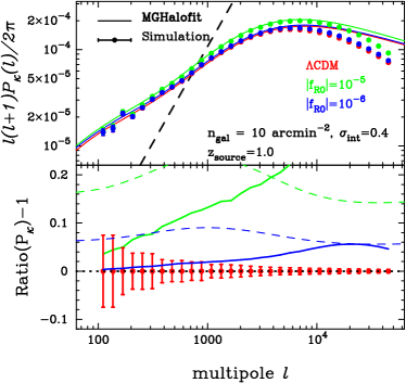
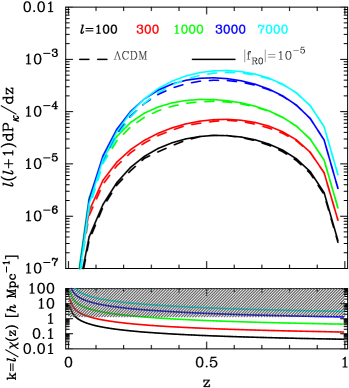
Figure 1: Impact of $f(R)$ gravity on the convergence power spectrum. Left: we show the dependence on $|f_{\rm R0}|$ of the convergence power spectrum. In the top panel, the colored points represent the average power spectrum over 100 realizations for the three models, while the bottom shows the relative difference between $\Lambda$CDM and the two $f(R)$ models. The black dashed line in the top panel corresponds to the shape noise contribution, while the colored lines are theoretical models based on a fitting formula of the three-dimensional matter power spectrum (Zhao, 2014). In the bottom panel, colored dashed line represents the relative difference of the convergence power spectrum for $\Lambda$CDM model when we vary the value of $\sigma_{8}$ to match to those in the $f(R)$ models. In the left-hand panels, the error bars represent the standard error of the average (i.e. the standard deviation of the each measurement divided by $\sqrt{100}$). Right: We show the integrand of the convergence power spectrum (16) as a function of redshift $z$. In the top panel, the dashed lines correspond to the $\Lambda$CDM case, while the solid lines are for the F5 model. There, different colored lines show the case of different multipoles as shown in the figure legend. In the lower panel, we show the comoving scale $k$ that contributes to the convergence power spectrum at the multipole $\ell$ at a given redshift $z$. As a reference, the grey hatched region represents the region where the linear matter perturbations would be enhanced by the additional scalar field degree of freedom.

Minkowski functionals

After constructing the smooth convergence field $\mathcal{K}$ on grid exactly as in the peak counts, we apply the following estimators of MFs, as shown in, e.g., Kratochvil et al. (2012),

$$V_{0}({\cal K}_{\rm thre}) = \frac{1}{A}\int\Theta(\mathcal{K}-{\cal K}_{\rm thre}){\rm d}x{\rm d}y,$$ (36)

$$V_{1}({\cal K}_{\rm thre}) = \frac{1}{4A}\int\delta_{D}(\mathcal{K}-{\cal K}_{\rm thre})\sqrt{\mathcal{K}_{x}^{2}+\mathcal{K}_{y}^{2}}{\rm d}x{\rm d}y,$$ (37)

$$V_{2}({\cal K}_{\rm thre}) = \frac{1}{2\pi A}\int\delta_{D}(\mathcal{K}-{\cal K}_{\rm thre})$$ (38)

$$\times \frac{2\mathcal{K}_{x}\mathcal{K}_{y}\mathcal{K}_{xy}-\mathcal{K}_{x}^{2}\mathcal{K}_{yy}-\mathcal{K}_{y}^{2}\mathcal{K}_{xx}}{\mathcal{K}_{x}^{2}+\mathcal{K}_{y}^{2}}{\rm d}x{\rm d}y,$$

where $\Theta(x)$ is the Heaviside step function and $\delta_{D}(x)$ is the Dirac delta function. The integrals in the above expressions are carried out by summing up the values over grid points specified by the sky coordinates $x$ and $y$. The subscripts on ${\cal K}$ represent differentiation with respect to these coordinates. The first and second differentiation are evaluated with finite difference. We compute MFs for 100 equally spaced bins of $(\mathcal{K}-\langle\mathcal{K}\rangle)/\sigma$ between $-10$ and $10$. We consider only the range $-3<(\mathcal{K}-\langle\mathcal{K}\rangle)/\sigma<4$ in the detectability analysis, for similar reasons to the peak counts. We will see shortly that a large amount of the sensitivity to the parameter $|f_{R0}|$ comes from this range.

5 RESULTS

5.1 Dependence of parameter in $f(R)$ gravity

Power spectrum

Let us first show the result of the convergence power spectrum $P_{\kappa}$. The left-hand panels in figure 1 summarize the average convergence power spectrum obtained from 100 ray-tracing maps. In both top and bottom panels, the red, green and blue points (or lines) correspond to the $\Lambda$CDM, F5 and F6 model, respectively. The red, green and blue solid lines in the top panel represent the corresponding theoretical predictions based on Eq. (16). To calculate Eq. (16) for the $f(R)$ models, we adopt the fitting formula of three-dimensional matter power spectrum as developed in Zhao (2014). Note that this fitting formula can reproduce the result in Takahashi et al. (2012) in the case of $|f_{\rm R0}|=0$. We find that the predication provides a reasonable fit to our simulation results for three different models in the range of $\ell\lower 2.15277pt\hbox{$\;\buildrel<\over{\sim}\;$}7000$. In the bottom panel, we show the relative difference of $P_{\kappa}$ between the $f(R)$ models and $\Lambda$CDM. The red error bars in the bottom panel corresponds to the standard error of the average convergence power spectrum for $\Lambda$CDM model. We confirm that the F5 and F6 models change the convergence power spectrum in the range of $\ell<7000$ by $\;\buildrel<\over{\sim}\;$20% and $\lower 2.15277pt\hbox{$\;\buildrel<\over{\sim}\;$}4\%$, respectively. In comparison, we also consider the relative difference of $P_{\kappa}$ between two $\Lambda$CDM models with different values of $\sigma_{8}$. The green dashed line in the bottom left-hand panel shows the relative difference between $\sigma_{8}=0.883$ and $0.830$, while the blue one is for the difference between $\sigma_{8}=0.845$ and $0.830$ (see also Table 1). While the overall level of the enhancement of power is similar to the modified gravity simulations, the trend in the dashed lines is quite different from that in the solid lines. Therefore, the convergence power spectrum can be a useful probe of $f(R)$ gravity whereas the effect is partly compensated by a change of $\sigma_{8}$.

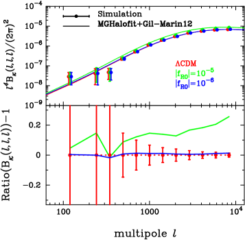
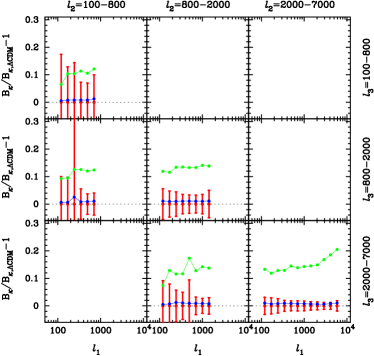
Figure 2: Impact of $f(R)$ gravity on the convergence bispectrum. Left: We show the dependence on $|f_{\rm R0}|$ of the convergence bispectrum for equilateral configuration with $\ell_{1}=\ell_{2}=\ell_{3}=\ell$. In the top panel, colored points represent the average bispectrum over 100 ray-tracing realizations for three models, while the bottom left one shows the relative difference between $\Lambda$CDM and the two $f(R)$ models. The colored solid line in the top panel shows the theoretical model based on Eq. (19) with the fitting formula in Gil-Marín et al. (2012). The error bars represent the standard error on the estimated average (i.e. the standard deviation divided by $\sqrt{100}$). Right: The relative difference of the convergence bispectrum between $\Lambda$CDM and the $f(R)$ models for more general triangular configurations $(\ell_{1},\ell_{2},\ell_{3})$ as shown on the axes. The red error bars show the standard error on the average bispectrum for $\Lambda$CDM model, while the green and blue lines are the ratio for F5 and F6 model, respectively. Note that we impose the condition of $\ell_{1}\leq\ell_{2}\leq\ell_{3}$ to count every triangle configuration once.

We further examine the contribution to $P_{\kappa}$ from the lens at a given redshift to understand when $f(R)$ gravity enhances the projected power the most significantly. The top right-hand panel in figure 1 shows the integrand in Eq. (16) using the fitting formula in Zhao (2014). Compared to $\Lambda$CDM, F5 model enhances the amplitude of the matter density fluctuations at $z\lower 2.15277pt\hbox{$\;\buildrel<\over{\sim}\;$}0.6$ for all the multipoles depicted here. In the bottom right panel, we show the wavenumber $k(z)=\ell/\chi(z)$ contributing in the calculation of Eq. (16) for a given redshift $z$. On linear scales where $\delta\rho_{m}\ll\bar{\rho}_{m}$, the Compton wavelength of the extra scalar field $f_{R}$ can be expressed as

$$\lambda_{C}^{-1}=\left(\frac{1}{3(n+1)}\frac{\bar{R}}{|f_{\rm R0}|}\left(\frac{\bar{R}}{\bar{R}_{0}}\right)^{n+1}\right)^{1/2}.$$ (39)

The grey hatched region in the bottom panel represents $k>a\lambda_{C}^{-1}$ where the fifth force due to $f_{R}$ can efficiently enhance the linear density fluctuations. Although the competition between the non-linear gravitational growth and the chameleon mechanism would make the situation more complicated, the criterion of $k>a\lambda_{C}^{-1}$ provides the typical scale where $f(R)$ gravity affects the density distribution. On large scales where $\ell\lower 2.15277pt\hbox{$\;\buildrel<\over{\sim}\;$}300$, the linear approximation works fairly well and the deviation from $\Lambda$CDM can be mainly explained by the scale-dependent linear growth rate. On the other hand, the chameleon mechanism does not completely suppress the effect of $f(R)$ gravity on the matter distribution on small scales.

Bispectrum

We next consider the convergence bispectrum $B_{\kappa}$. Figure 2 summarizes the simulation results obtained from 100 ray-tracing maps for the three different models with $|f_{\rm R0}|=0,10^{-6}$ and $10^{-5}$. In the left-hand panels, we show the result of $B_{\kappa}$ for the equilateral triangle configuration with $\ell_{1}=\ell_{2}=\ell_{3}=\ell$. First of all, we compare the simulation result for the $\Lambda$CDM model and the theoretical prediction. In the calculation, we adopt the fitting formula of the three-dimensional matter bispectrum $B_{\delta}$ proposed in Gil-Marín et al. (2012) and plug it into Eq. (19). This fitting formula explicitly includes the three-dimensional matter power spectrum and we use the fitting formula in Zhao (2014) (which is equivalent to (Takahashi et al., 2012) for $\Lambda$CDM) for that. We find that the fitting formula is in good agreement with the simulation results again over the range of $\ell\lower 2.15277pt\hbox{$\;\buildrel<\over{\sim}\;$}7000$ for $\Lambda$CDM model. This result is consistent with a previous work by Sato & Nishimichi (2013). For $\ell\lower 2.15277pt\hbox{$\;\buildrel<\over{\sim}\;$}300$, the difference between the simulation results and the analytic models appears to be relatively large, mildly larger than the error bars estimated from the scatter among realizations. This is possibly because we repeatedly use a single $N$-body simulation to generate a quasi-independent ensemble and thus the quoted error level might be not very accurate. Another reason for the small discrepancy is the finite area of the simulated maps. This can be expressed as a convolution with a window function corresponding to the $5^{\circ}\times 5^{\circ}$ geometry, and this corresponds to $\ell=360/5=72$ in multipole. The low-$\ell$ data points are not so far from this typical length scale. Furthermore, the fitting formula can also provide a reasonable fit to both F5 and F6 models, even though the fitting formula for $B_{\delta}$ is constructed for a $\Lambda$CDM cosmology by numerical simulations. In order to quantify the effect of $|f_{\rm R0}|$ on $B_{\kappa}$, we also show the relative difference of the bispectrum between the $\Lambda$CDM and the $f(R)$ models in the left-hand bottom panel and the right-hand panels of Figure 2. The bottom left-hand panel represents the result for the equilateral configuration, while the right-hand panels summarize more general configurations specified by three multipoles, $\ell_{1}\leq\ell_{2}\leq\ell_{3}$. In the right panels, we reduce the number of bins for $\ell_{2}$ and $\ell_{3}$ to show the effect of $|f_{\rm R0}|$ in an easy to see manner. Overall, we find that the F5 model affects the convergence bispectrum by $\lower 2.15277pt\hbox{$\;\buildrel<\over{\sim}\;$}20\%$ and the dependence on the triangle shape is rather weak except for $\ell_{i}\lower 2.15277pt\hbox{$\;\buildrel>\over{\sim}\;$}2000$. On the other hand, we can not find significant deviation from the $\Lambda$CDM for F6 model. Although the effect of $|f_{\rm R0}|$ on $B_{\kappa}$ seems similar to that on $P_{\kappa}$ for the angular scale of $\ell\lower 2.15277pt\hbox{$\;\buildrel<\over{\sim}\;$}2000$, the statistical uncertainty of $B_{\kappa}$ would be larger than $P_{\kappa}$, implying that the bispectrum would be less sensitive to $f(R)$ gravity and provide a weaker constraint on $|f_{\rm R0}|$ compared to the power spectrum. We revisit the constraining power on $|f_{\rm R0}|$ with cosmic shear statistics in Section 5.2. Nevertheless, we should note that $B_{\kappa}$ would play an important role to break the degeneracy among cosmological parameters such as $\Omega_{\rm m0}$ and $\sigma_{8}$ in cosmic shear analyses.

Peak count

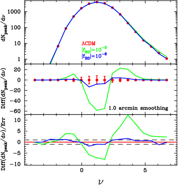
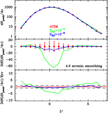
Figure 3: Impact of $f(R)$ gravity on the peak counts. Left: We show the dependence of the peak counts on $|f_{\rm R0}|$. In the top panel, the red points represent the average (differential) number density of peaks over 100 realizations for the $\Lambda$CDM model, while the green and blue lines are for the F5 and F6 models. The middle one shows the difference between $\Lambda$CDM and $f(R)$ models, while the bottom is for the difference normalized by the standard error of average for the $\Lambda$CDM model. Right: Similar to the left panel, but larger smoothing scale of 4.5 arcmin is adopted. In both panels, the error bars represent the standard error of the average (i.e. the standard deviation divided by $\sqrt{100}$). Note that the error level corresponds to $100\times{(5\,\mathrm{deg})^{2}}=2,500\,\mathrm{deg}^{2}$.

We here summarize the results of the peak counts. We define the differential number density of peaks and then compare the results among three different models. Figure 3 shows the effect of $f(R)$ gravity on the peak counts. The left-hand panel represents the simulation results with the smoothing scale of 1 arcmin, while the right-hand panel are for the smoothing with $\theta_{G}=4.5$ arcmin. In both panels, red, green and blue points (or lines) represent the average of number density of peaks for $\Lambda$CDM, F5, and F6 models, respectively. As in Figure 1, we show the difference of the number density in the middle panels, while we normalize the difference by the standard error of average for the $\Lambda$CDM model in the bottom panels. We find that the effect of $f(R)$ gravity on the peak counts appears in not only $\nu\geq 3$ but also $\nu\sim 1$. The peaks with $\nu\geq 3$ correspond to isolated massive dark matter halos along the line of sight [see Fan et al. (2010) for analytical estimate of the shape-noise contamination on these peaks and also Higuchi & Shirasaki (2016) for the detailed comparisons in $f(R)$ model]. General trend of the number density among three models is found to be consistent with the expectation from the halo mass function (e.g., Shirasaki et al., 2016). The number density of high peaks increases in the range of $\nu\geq 3$ in the HS model. These specific features would reflect the non-trivial dependence of halo mass function on $|f_{\rm R0}|$ (e.g., Li & Hu, 2011; Li & Efstathiou, 2012; Lombriser et al., 2013; Cataneo et al., 2016). With a larger smoothing scale, which roughly corresponds to the removal of Fourier modes with $\ell\lower 2.15277pt\hbox{$\;\buildrel>\over{\sim}\;$}2000$, a bumpy feature at $\nu\sim 3.5$ for the F5 model disappears. For larger $\theta_{G}$, the halo-peak correspondence gets worse because sharp structures such as halos are erased by the smoothing operation. This would indicate that the simple framework presented in Shirasaki et al. (2015) can not explain the number count of peaks on $\nu>3$ as $\theta_{G}$ would become larger. Also, we find the number density at $\nu\sim 1$ is significantly changed from $\Lambda$CDM when we set $|f_{\rm R0}|=10^{-5}$. This could originate from the larger density fluctuations in F5 and F6 models expressed in terms of $\sigma_{8}$ (Kratochvil et al., 2010) or the superposition of less massive objects (Yang et al., 2011). Although it is still not straightforward to physically interpret these low-S/N peaks and thus it might be safer to avoid them in cosmological tests, we would like to stress here that they do have sensitivity to the parameter $|f_{\rm R0}|$ in a statistical sense, even in the presence of realistic shape noise. We reserve the study on the degeneracy between $|f_{\rm R0}|$ and $\sigma_{8}$ in peak counts in Section 5.3.

Minkowski functionals

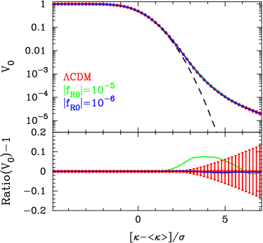
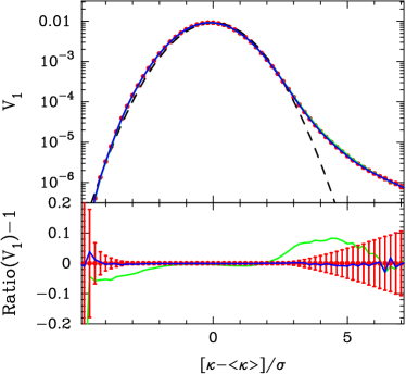
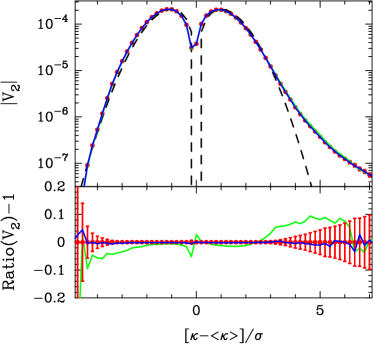
Figure 4: Impact of $f(R)$ gravity on the Minkowski functionals (MFs). The three panels represent the results of $V_{0}$, $V_{1}$ and $V_{2}$. In every panel, the error bars represent the standard error of the average (i.e. the standard deviation divided by $\sqrt{100}$). Also, colored points represent the average MF over 100 realizations for the three models, while the bottom portion shows the relative difference of MF between $\Lambda$CDM and $f(R)$ models. The dashed line shows the Gaussian prediction for $\Lambda$CDM model.

We then present the measurements of the lensing MFs obtained from 100 simulations. Figure 4 summarizes the effect of $|f_{\rm R0}|$ on the lensing MFs. First of all, we confirm the non-Gaussian feature in lensing MFs for the three models even when we add the shape noise for which we assume Gaussian distribution. The shape of the MFs obtained from simulations can not be explained by the Gaussian expectation in Eqs. (32)-(34) depicted by the dashed lines, implying that the lensing MFs are useful probe of non-Gaussian nature of the convergence field that can not be captured by the power spectrum. Our results are broadly consistent with a previous work by Ling et al. (2015). In the case of F5 model, we find that the deviation from $\Lambda$CDM is at most $\sim 10\%$ and the clear deviations are found at $x=({\cal K}-\langle{\cal K}\rangle)/\sigma\sim 2-5$. On the other hand, we find only $\lower 2.15277pt\hbox{$\;\buildrel<\over{\sim}\;$}1\%$ differences between F6 and $\Lambda$CDM models. Note that the deviation from the $\Lambda$CDM we observe is found to be smaller than Ling et al. (2015) have shown. One of the reasons behind this trend is in the difference of the adopted values of $|f_{\rm R0}|$ and other cosmological parameters. The model parameters used in Ling et al. (2015) are different despite the same label: their F5 means $|f_{\rm R0}|=1.29\times 10^{-5}$ instead of $10^{-5}$. They also adopted smaller $\Omega_{\rm m0}$ and $\sigma_{8}$, both indicating weaker screening and therefore stronger deviation from GR for the same $|f_{\rm R0}|$. Besides, the difference between our result and previous one would be partly explained by the projection effect. Our simulations include the projection effect and the shape noise simultaneously, while Ling et al. (2015) have focused on the surface mass density at $z=0.1$. Furthermore, we find that the difference of the lensing MFs between the $\Lambda$CDM and the HS model has the similar trend to a change of $\sigma_{8}$ (e.g., see Figure 2 in Shirasaki & Yoshida, 2014).

5.2 Detectability of imprint of $f(R)$ gravity

In order to quantify the detectability of $f(R)$ gravity in a given statistical quantity, we start by writing a measure of a goodness-of-fit;

$$\chi^{2} = \sum_{i,j}{\bf C}^{-1}_{ij}\left[{\cal O}(x_{i};true)-{\cal M}(x_{i};test)\right]$$ (40)

$$\,\,\,\,\,\,\,\,\,\,\,\,\,\,\,\,\,\,\,\,\,\,\,\,\,\times\left[{\cal O}(x_{j};true)-{\cal M}(x_{j};test)\right],$$

where ${\cal M}(x_{i};test)$ represents a theoretical model of cosmic shear statistic at the $i$-th bin of $x$ for a cosmological model that one wishes to test, ${\cal O}(x_{i};true)$ is an observed statistic drawn from the true unknown cosmology, and ${\bf C}$ is the covariance matrix of the observed data vector ${\cal O}$. In our case, ${\cal O}$ corresponds to either the power spectrum, bispectrum, peak counts or MFs, while $x$ refers to the multipole $\ell$, the peak height $\nu$, or the normalized convergence $({\cal K}-\langle{\cal K}\rangle)/\sigma$ depending on the statistics. In what follows, we also consider a data vector ${\cal O}$ composed of different statistics when we examine parameter constraints from joint analyses of more than one statistic. In such cases, we properly take into account the off-diagonal components relevant to the two statistics of interest in the covariance matrix.

When ${\cal O}$ follows a multi-variate Gaussian distribution and if we assume the correct model in $\mathcal{M}(x_{i};test)$, the quantity defined by Eq. (40) follows the $\chi^{2}$ distribution with the degree of freedom of $N_{\rm bin}-1$ as the name suggests, where $N_{\rm bin}$ represents the total number of bins for the observables ${\cal O}$. Borrowing the idea behind Eq. (40), which compares the levels of estimated (in the form of a covariance matrix) and measured (the actual scatter around the mean) cosmic variances, we define a similar quantity to assess the statistical power to constrain $|f_{\rm R0}|$ by replacing the numerator with the difference of the expected statistics in two models:

$$\left({\rm S/N}\right)^{2} = \sum_{i,j}{\bf C}^{-1}_{ij}\left[{\cal M}(x_{i};|f_{\rm R0}|)-{\cal M}(x_{i};\Lambda{\rm CDM})\right]$$ (41)

$$\,\,\,\,\,\,\,\,\,\,\,\times\left[{\cal M}(x_{j};|f_{\rm R0}|)-{\cal M}(x_{j};\Lambda{\rm CDM})\right],$$

where we consider the $f(R)$ cosmology characterized by $|f_{\rm R0}|$ and the fiducial $\Lambda$CDM cosmology.

One can assess the discriminating power of the statistic by the $({\rm S/N})^{2}$ defined above. Note that this quantity does not depend on the binning scheme explicitly, as long as we take a binning fine enough not to miss important features in the statistics. In the absence of degeneracy between different cosmological parameters, one can straightforwardly convert the $({\rm S/N})^{2}$ to the expected level of constraint on $|f_{R0}|$; $({\rm S/N})^{2}=4$ for $|f_{R0}|=10^{-5}$ corresponds to $\sigma_{|f_{R0}|}=10^{-5}/\sqrt{4}=5\times 10^{-6}$, for instance. Note that we consider the degeneracy among cosmological parameters in Section 5.3 in details.

In Eq (41), we estimate ${\cal M}(x_{i};|f_{\rm R0}|)$ and ${\cal M}(x_{i};\Lambda{\rm CDM})$ as the ensemble average over 100 realizations of our ray-tracing maps as shown in Section 4.1. To derive accurate covariance matrices of these observables and the cross covariance between two different observables, we also make use of the 1000 ray-tracing simulations performed by Sato et al. (2009). The maps in Sato et al. (2009) have almost the same design as our simulations, but are generated for slightly different cosmological parameters [consistent with Wilkinson Microwave Anisotropy Probe (WMAP) 3-year results (Spergel et al., 2007)]. We use the maps with a sky coverage of $5\times 5\,{\rm deg}^{2}$ for $z_{\rm source}=1$. In order to estimate cosmic shear statistics, we properly take into account the contamination from the intrinsic shape of sources by adding a Gaussian noise to shear (also see Section 4.1). For a given observable ${\cal O}$, we estimate the covariance matrix using the 1000 realizations of ray-tracing simulations as follows;

$${\bf C}_{ij} = \frac{1}{N_{\rm rea}-1}\sum_{r=1}^{N_{\rm rea}}\left[{\cal O}^{(r)}(x_{i})-\bar{{\cal O}}(x_{i})\right]$$ (42)

$$\,\,\,\,\,\,\,\,\,\,\,\,\,\,\,\,\,\,\,\,\,\,\,\,\,\,\,\,\,\,\,\,\,\,\,\,\,\,\,\,\,\,\,\,\,\times\left[{\cal O}^{(r)}(x_{j})-\bar{{\cal O}}(x_{j})\right],$$

$$\bar{{\cal O}}(x_{i}) = \frac{1}{N_{\rm rea}}\sum_{r=1}^{N_{\rm rea}}{\cal O}^{(r)}(x_{i}),$$ (43)

where $N_{\rm rea}=1000$ and ${\cal O}^{(r)}(x_{i})$ is the observable obtained from $r$-th realization of simulations for $i$-th bin of $x$. When we calculate the inverse covariance matrix, we multiply a debiasing correction, $\alpha=(N_{\rm rea}-N_{\rm bin}-2)/(N_{\rm rea}-1)$, with $N_{\rm rea}=1000$ and $N_{\rm bin}$ being the number of total bins in our data vector (Hartlap et al., 2007). In the following, we assume that the covariance matrix is scaled as the inverse of the survey area and consider a hypothetical lensing survey with a sky coverage of $1500\,{\rm deg}^{2}$, which corresponds to the ongoing imaging survey with Subaru Hyper Suprime-Cam(Miyazaki et al., 2006). Note that under the assumed scaling of the covariance matrix, one can easily calculate the corresponding $({\rm S/N})^{2}$ for a given sky coverage of $A\,{\rm deg}^{2}$ by multiplying the $({\rm S/N})^{2}$ presented in this section by a factor of $A/1,500$. Table 2 summarizes the results of this section.

Table 2: Summary of the signal-to-noise ratio among cosmic shear statistics. We show $({\rm S/N})^{2}$ defined by Eq. (40). We show the results for $|f_{R0}|=10^{-5}$ in the upper half, and for $|f_{R0}|=10^{-6}$ in the bottom half. In addition to the fiducial analysis, we also show the results when we increase the smoothing scale to $\theta_{G}=4.5\,{\rm arcmin}$, or the source number density is set to $n_{\rm gal}=30\,{\rm arcmin}^{-2})$. All values are for the sky coverage of 1,500 squared degrees.

	$P_{\kappa}$	$B_{\kappa}$	Peak	MFs	$P_{\kappa}+B_{\kappa}$	$P_{\kappa}+$Peak	$P_{\kappa}+$MFs
$|f_{\rm R0}|=10^{-5}$
Fiducial analysis	127.6	45.1	121.7	1000.9	130.5	201.6	1066.0
Larger smoothing scale	127.6	45.1	53.5	35.3	130.5	151.1	185.1
Higher source number density	255.1	73.9	608.2	2837.2	264.5	668.6	2972.2
$|f_{\rm R0}|=10^{-6}$
Fiducial analysis	2.63	0.301	4.85	4.28	2.64	6.52	6.51
Larger smoothing scale	2.63	0.301	1.39	0.237	2.64	3.37	3.45
Higher source number density	5.44	0.540	29.0	19.3	6.49	30.3	27.3

Fiducial analysis

As the fiducial analysis, we consider a situation in which the two spectra $P_{\kappa}$ and $B_{\kappa}$ are measured in the range of $100\leq\ell\leq 2000$, while we have the number density of peaks in the range of $-2<\nu<4$ and MFs are given for $-3\leq({\cal K}-\langle{\cal K}\rangle)/\sigma\leq 4$. For the two convergence spectra, we adopt the same binning as summarized in Section 4.2, leading to 14 bins for $P_{\kappa}$ and 78 bins for $B_{\kappa}$ in total. On the other hand, we construct the number density of peaks in 10 bins with width of $\Delta\nu=0.6$, while we employ 12 bins to measure each lensing MF.

As shown in Table 2, the values of $({\rm S/N})^{2}$ indicates that all the cosmic shear statistics considered here can distinguish the F5 model from the $\Lambda$CDM model with a high significance level when the other cosmological parameters are fully known. Even a very small modification to GR such as our F6 model is detectable by these statistics except when we employ the bispectrum alone. Surprisingly, non-standard statistics such as the peak counts or the MFs have very high signal-to-noise ratio competitive or significantly larger than the conventional analyses using the power or bispectra (Liu et al., 2016). This indicates that the weak lensing convergence field indeed exhibits strong non-Gaussianity that is difficult to capture by low-order polyspectra. Geometrical measures such as the MFs are especially powerful in such a regime. We also find the $({\rm S/N})^{2}$ from combined analyses with two statistics is slightly smaller than the simple sum of the individual values (the three right-hand columns). This is due to the cross covariance between the statistics. While we can access independent information through different measures reflecting an increase in the $({\rm S/N})^{2}$ from the combined analyses, part of it is common to that in the power spectrum. This demonstrates the importance of a proper account of the cross-covariance in actual data analyses.

Dependence on smoothing scale and shape noise

We have seen so far the statistical power of four different measures in testing the possibility of modified gravity. Among the four statistics, the power and the bispectra are given explicitly as a function of the physical scale. Since we expect that smaller scales are more severely contaminated by e.g., intrinsic alignment or baryonic physics, we can conduct a more reliable cosmological test by limiting ourselves in large scales. On the other hand, the dependence of the peak counts and the MFs on the physical scale is less clear. What we have done so far is based on the statistics at one given scale $\theta_{G}=1\,{\rm arcmin}$, chosen to have a good correspondence between peaks and massive clusters. We thus investigate in this section the dependence of the detectability of a non-zero $|f_{R0}|$ on the smoothing scale that defines the peaks and MFs. We also test the dependence on the mean density of source galaxies, which can alter the result significantly.

We first examine the dependence on the smoothing scales by setting $\theta_{G}=4.5\,{\rm arcmin}$, which roughly corresponds to $\ell=2000$. For this choice of smoothing, all the four statistics probe roughly the same angular scale and thus we expect that they have a similar level of theoretical uncertainties due to small scale effects. In this sense, we can do a fairer comparison among the four. The results are shown in Table 2 both for $|f_{R0}|=10^{-5}$ and $10^{-6}$. Compared to the fiducial analysis with $\theta_{G}=1\,{\rm arcmin}$, the level of non-Gaussianity in the smoothed map is strongly suppressed. As a result, the S/N from the lensing MFs is greatly reduced. The statistical power of the peak counts is also suppressed, but to a much lesser extent. When we combine these statistics with the power spectrum, we have a larger increase in the S/N for the MFs than for peak counts, because there is a larger overlap in information for the peak counts and the power spectrum with this choice of $\theta_{G}$. Although we lose significant $({\rm S/N})^{2}$ in the MFs, they still probe independent information to the power spectrum.

Another test is a larger source number density with the smoothing scale unchanged. We consider 30 ${\rm arcmin}^{-2}$, and this leads to the shape noise level reduced by a factor of $1/\sqrt{3}\sim 0.57$. We reanalyse the power and the bispectra in addition to the peak counts and the MFs in this case. We can see in Table 2 that such a deeper imaging survey with a higher source number density provides a significantly improved S/N. Especially, the peak counts and lensing MFs are sensitive to the number density. We find that $({\rm S/N})^{2}$ for peak counts and MFs increases by a factor of $\sim 5$ and $\sim 2.8$, respectively. Provided that the small scale uncertainties are well under control, these two statistics have a potential to distinguish the F5 or even F6 model from the $\Lambda$CDM model with a very high significance in upcoming deep imaging surveys.

5.3 Degeneracy among cosmological parameters

We then study the degeneracy between $|f_{\rm R0}|$ and cosmological parameters. Cosmic shear observables depend sensitively on the two parameters of $\Omega_{\rm m0}$ and $\sigma_{8}$ through Eq. (14). Thus, we focus on these parameters and investigate how well we can constrain $|f_{\rm R0}|$ when these parameters are jointly varied. We first construct a model of the parameter dependence of cosmic shear statistic ${\cal O}(x)$ by expanding into the Taylor series around a fiducial point $(\Omega_{\rm m0,fid},\sigma_{8,{\rm fid}},|f_{\rm R0}|=0)$:

$${\cal O}(x_{i};\Omega_{\rm m0},\sigma_{8},|f_{\rm R0}|) \simeq {\cal O}(x_{i};\Omega_{\rm m0,fid},\sigma_{8,{\rm fid}},|f_{\rm R0}|=0)$$ (44)

$$+\frac{\partial{\cal O}(x_{i})}{\partial\Omega_{\rm m0}}(\Omega_{\rm m0}-\Omega_{\rm m0,fid})$$

$$+\frac{\partial{\cal O}(x_{i})}{\partial\sigma_{8}}(\sigma_{8}-\sigma_{8,{\rm fid}})$$

$$+\frac{\partial{\cal O}(x_{i})}{\partial|f_{\rm R0}|}|f_{\rm R0}|,$$

where $\Omega_{\rm m0,fid}=0.315$, $\sigma_{8,{\rm fid}}=0.830$, and the first derivatives are estimated from the five simulations at the bottom of Table 1 by the finite difference method (both-sided for $\Omega_{\rm m0}$ and $\sigma_{8}$, and one-sided for $|f_{\rm R0}|$).

Figure 5 summarizes our cosmic shear statistics as a function of $|f_{\rm R0}|$, $\Omega_{\rm m0}$ and $\sigma_{8}$. In this section, we consider the same binning of observables as in the fiducial analysis in Section 5.2. Figure 5 shows the fractional difference of cosmic shear statistic compared to the fiducial model. The green and blue lines in the figure represent the ratio for F5 and F6 model, respectively. The black solid and dashed lines are for $\Lambda$CDM with higher $\Omega_{\rm m0}$ and $\sigma_{8}$. For visualization, we classify the triangular configuration of the arguments of the convergence bispectrum into equilateral $(\ell_{1}=\ell_{2}=\ell_{3})$, isosceles $(\ell_{1}=\ell_{2})$, and scalene $(\ell_{1}\neq\ell_{2}\neq\ell_{3})$. The grey error bars represent the statistical uncertainty in a hypothetical survey with 1,500 squared degrees estimated from the 1000 ray-tracing simulations in Sato et al. (2009). As a whole, the dependence of $|f_{\rm R0}|$ is found to be quite similar to that of $\Omega_{\rm m0}$ and $\sigma_{8}$ because $f(R)$ model predicts a higher $\sigma_{8}$ for a fixed amplitude of initial curvature perturbations and cosmic matter density through a more rapid growth of structure.

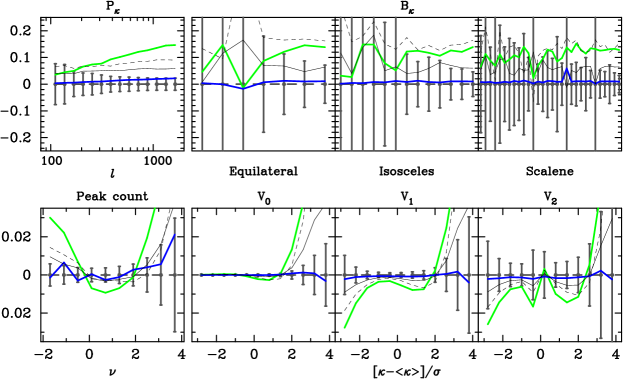
Figure 5: Degeneracy between cosmological parameters and $f(R)$ gravity. Each panel represents the relative difference of one of a various cosmic shear statistics between the fiducial $\Lambda$CDM model and the other models. The green and blue lines correspond to the F5 and F6 model, respectively. On the other hand, the black solid line shows the case of $\Lambda$ CDM with $\Omega_{\rm m0}$ larger by 0.025, while the black dashed line is for a model with $\sigma_{8}$ larger by 0.050. Note that the grey error bars in each panel correspond to the cosmic variance from a survey with the sky coverage of 1,500 squared degrees. The detailed configuration of triangles in bispectrum is summarized in Appendix.

Table 3: Expected constraint on $|f_{R0}|$ from Fisher analysis for various statistics. We show the $1$-$\sigma$ error level in units of $10^{-6}$, assuming the fiducial survey parameters; $\theta_{G}=1\,{\rm arcmin}$, $n_{\rm gal}=10\,{\rm arcmin}^{-2}$ and $1,500$ squared degrees. We consider both unmarginalized and marginalized cases over $\Omega_{\rm m0}$ and $\sigma_{8}$. We adopt the maximum multipole for the power and the bispectra to be $\ell_{\mathrm{max}}=2,000$ in the top two rows, while the bottom two rows include information on smaller scales up to $\ell_{\mathrm{max}}=8,000$, which probes roughly consistent length scales to the peak counts and the MFs.

	$P_{\kappa}$	$B_{\kappa}$	Peak	MFs	$P_{\kappa}+B_{\kappa}$	$P_{\kappa}+$Peak	$P_{\kappa}+$MFs	$P_{\kappa}+B_{\kappa}+$Peak	$P_{\kappa}+B_{\kappa}+$MFs	all
unmarginalized	0.616	1.799	0.454	0.483	0.615	0.392	0.392	0.398	0.398	0.281
marginalized	3.069	3.980	0.565	0.936	1.400	0.546	0.802	0.533	0.753	0.409
unmarginalized	0.394	1.21	0.454	0.483	0.405	0.317	0.310	0.329	0.327	0.262
marginalized	1.29	2.46	0.565	0.936	0.607	0.522	0.634	0.431	0.522	0.365

The Fisher matrix approach provides a quantitative method to evaluate the importance of degeneracy among cosmological parameters. The Fisher matrix $F_{\alpha\beta}$ is given by

$$F_{\alpha\beta}=\sum_{ij}{\bf C}_{ij}^{-1}\frac{\partial{\cal O}(x_{i})}{\partial p_{\alpha}}\frac{\partial{\cal O}(x_{j})}{\partial p_{\beta}},$$ (45)

where $p_{\alpha}$ and $p_{\beta}$ run for cosmological parameters (i.e., $|f_{\rm R0}|$, $\Omega_{\rm m0}$ and $\sigma_{8}$ in our case). Note that we ignore the cosmological dependence of the covariance matrix in Eq (45). We here consider two error levels; un-marginalized error of $|f_{\rm R0}|$ and marginalized error of $|f_{\rm R0}|$ considering $\Omega_{\rm m0}$ and $\sigma_{8}$. The former corresponds to the case in which the parameters $\Omega_{\rm m0}$ and $\sigma_{8}$ (or the amplitude of the primordial fluctuations, $A_{s}$, in realistic situations) are already constrained very tightly from independent observations, while the latter takes into account the effect of parameter degeneracy on error estimate. Thus, we can see the importance of parameter degeneracy by comparing the un-marginalized and marginalized errors.

Table 3 summarizes both un-marginalized and marginalized errors of $|f_{\rm R0}|$ for a hypothetical imaging survey with the sky coverage of 1,500 squared degrees. The two upper rows correspond to our fiducial case with $\ell_{\rm max}=2,000$ and $\theta_{G}=1$ arcmin. According to the Fisher analysis, the power-spectrum analysis results in the most degraded constraint on $|f_{\rm R0}|$ after marginalization over $\Omega_{\rm m0}$ and $\sigma_{8}$; the error level gets $\sim 5$ times larger. Although the other cosmic shear statistics do also suffer from parameter degeneracy, combinations of two or more observables can improve the situation quite significantly. We can confirm in the table that the parameter degeneracy is gradually broken by adding statistics one by one. By properly using the four cosmic shear statistics presented in this paper, one can provide a better marginalized constraint on $|f_{\rm R0}|$ than the un-marginalized error expected from the power-spectrum analysis alone. These results would demonstrate the importance of use of different cosmic shear statistics in upcoming imaging surveys.

So far, our discussion is based on the fiducial analysis. It is, then, of importance to quantify the constraining power from different physical scales. Indeed, the maximum multipole $\ell_{\rm max}=2,000$ used in the power and the bispectra and the smoothing scale $\theta_{G}=1$ arcmin for the peak counts and MFs correspond to somewhat different length scales as we already mentioned earlier. We now change the former to $\ell_{\rm max}=8,000$ to roughly match to $\theta_{G}=1$ arcmin. Note that this choice is a bit too aggressive given the larger uncertainties both in theoretical modelling and measurements. We show this ideal case only to see the information on the gravity theory in different statistics from a fair comparison at similar scales.

The resulting constraints on $|f_{\rm R0}|$ are listed in the bottom two rows of Table 3. The bottom line is the same as the fiducial analysis; the conventional power-spectrum analysis exhibits the most notable degradation of the constraint on $|f_{\rm R0}|$, and this is mitigated by combining more and more statistics. Now, thanks to the small-scale information from the power and the bispectra, the error level from each of the statistics is very similar.

Although Figure 5 shows clear degeneracy among three parameters of $|f_{\rm R0}|$, $\Omega_{\rm m0}$ and $\sigma_{8}$ in cosmic shear statistics, the effect of $|f_{\rm R0}|$ is not compensated by different $\Omega_{\rm m0}$ and $\sigma_{8}$ exactly. For instance, the scale-dependent linear growth rate and the specific feature in the halo mass function in the $f(R)$ model are quite unique and thus difficult to absorb by a change in $\Omega_{\rm m0}$ and $\sigma_{8}$ within the $\Lambda$CDM scenario.

In order to demonstrate this situation more quantitatively, we consider the effective bias on the $\Omega_{\rm m0}-\sigma_{8}$ plane assuming the F6 model is the true cosmological model that governs the universe but $\Lambda$CDM model is wrongly adopted in the data analysis. We estimate the bias in parameter estimation as (Huterer et al., 2006)

$$\delta p_{\alpha}=\sum_{\beta}F_{{\rm GR},\alpha\beta}^{-1}\left[{\cal O}(x_{i};{\rm F6})-{\cal O}(x_{i};{\rm fid})\right]{\bf C}^{-1}_{ij}\frac{\partial{\cal O}(x_{j})}{\partial p_{\beta}},$$ (46)

where $p_{\alpha}=(\Omega_{\rm m0},\sigma_{8})$, ${\cal O}(x_{i};{\rm fid})$ represents the assumed $\Lambda$CDM model, while ${\cal O}(x_{i};F6)$ is the true cosmological model, corresponding to the F6 model in this case. The matrix of $F_{{\rm GR},\alpha\beta}$ in Eq. (46) is the Fisher matrix for $\Omega_{\rm m0}$ and $\sigma_{8}$, and is the sub-matrix of that in Eq (45). The Fisher matrix $F_{{\rm GR},\alpha\beta}$ provides the confidence region around the fiducial $\Lambda$CDM parameter. If the difference of the cosmic shear statistics between F6 and $\Lambda$CDM models can be explained by simply the difference in $\sigma_{8}$, the bias by Eq (46) would be equal to the difference of two values of $\sigma_{8}$ in these models. More specifically, the bias on $\Omega_{\rm m0}-\sigma_{8}$ plane would be equal to $(\delta\Omega_{\rm m0},\delta\sigma_{8})=(0,\sigma_{8}({\rm F6})-\sigma_{8}(\Lambda{\rm CDM}))$, where $\sigma_{8}(\rm F6)$ represents the resulting $\sigma_{8}$ in F6 model, and so on.

Figure 6 shows the result of this analysis. While we show the standard Fisher analysis within the $\Lambda$CDM framework in the left-hand panel, we show in the right-hand panel the biased estimation in $\Omega_{\rm m0}-\sigma_{8}$ plane induced by the difference between F6 and $\Lambda$CDM model. We show the 95% confidence region estimated from the Fisher matrix with an ideal future survey with the sky coverage of 20,000 squared degrees. The centers of ellipses in the right-hand panel are off from the true position depicted by the crossing point of the horizontal and the vertical dotted lines, and the displacement from that point shows the effective bias given by Eq. (46). For simplicity, we employ the size the ellipses the same as in the left-hand panel. We also show by the grey star symbol the expected central value if the difference between F6 and $\Lambda$CDM can completely be explained by the change in $\sigma_{8}$.

According to the right-hand panel, we find that the effect of $f(R)$ gravity on the power spectrum would be mainly determined by the change of $\sigma_{8}$, but the other statistics suggest that the difference also propagates to the estimated $\Omega_{\rm m0}$. Since the convergence bispectrum is less sensitive to $|f_{\rm R0}|$, the bias from using it alone on $\Omega_{\rm m0}-\sigma_{8}$ plane would be smaller than the statistical uncertainty in a survey of 20,000 squared degrees. This implies that it is difficult to distinguish the F6 model from $\Lambda$CDM model with bispectrum alone. Interestingly, peak counts and lensing MFs would predict higher $\Omega_{\rm m0}$ and lower $\sigma_{8}$ if F6 is the true model. The amount of bias in lensing MFs is smaller than the one in peak counts, because of different sensitivity of $|f_{\rm R0}|$ as shown in Section 5.2.

The result indicates that one can eventually find a clue beyond the $\Lambda$CDM model by detecting discrepancies in the allowed parameter regions from multiple statistics. Notably, a realistic analysis of the power and the bispectra up to $\ell_{\rm max}=2,000$ can find this with a high significance for a value of $|f_{\rm R0}|$ as small as $10^{-6}$. The additional statistics such as the peak counts and the MFs would provide an even more promising path towards the law of gravity on cosmological scales.

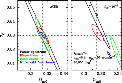
Figure 6: Consistency among cosmic shear statistics. In the left-hand panel, we show the 95% confidence region of $(\Omega_{\rm m0},\sigma_{8})$ for $\Lambda$CDM. In the right-hand panel, we represent the bias on the $\Omega_{\rm m0}-\sigma_{8}$ plane when F6 model is the true model but we use $\Lambda$CDM model in parameter constraints. The grey star point in the right panel is the expected bias assuming that the difference of statistics between F6 and $\Lambda$CDM can be explained by difference of $\sigma_{8}$. In both panels, colored symbols correspond to different cosmic shear statistics (black for power spectrum, red for bispectrum, green for peak counts, and blue for MFs). In this figure, we assume the sky coverage of 20,000 squared degrees and the source number density of 30 ${\rm arcmin}^{-2}$.

6 CONCLUSION AND DISCUSSION

In this paper, we studied the effects of $f(R)$ gravity on statistical properties of the weak gravitational lensing field. For this purpose, we have performed $N$-body simulations to investigate structure formation in a universe under the $f(R)$ model proposed in HS model. We then employed ray-tracing method to realize a realistic situation of weak lensing measurements in galaxy imaging survey. In ray-tracing simulations, we have properly taken into account the deflection of light along the line of sight and galaxy shape noise. The large set of these mock lensing catalogs enables us to study the information content about $f(R)$ gravity in cosmic shear statistics which have already been conducted in previous imaging surveys. Our main findings are summarized as follows:

1. The convergence power spectrum contain information about $f(R)$ gravity because of the scale-dependent linear growth rate and the environment-dependence of non-linear gravitational growth. Assuming the source redshift is set to be 1, $f(R)$ gravity would enhance the amplitude of the spectrum at $\ell=1000$ with a level of $\sim 12\%$ and $2\%$ for $|f_{\rm R0}|=10^{-5}$ and $10^{-6}$, respectively. Although the change of convergence power spectrum is expected given by the difference of $\sigma_{8}$ between $f(R)$ and $\Lambda$CDM models, correct understanding of the non-linear gravitational growth in $f(R)$ gravity would be required to determine the amplitude accurately (e.g., Zhao, 2014).

2. The convergence bispectrum is the lowest-order non-Gaussian information in weak lensing field. We find that it can change by $\sim 10\%$ with the model of $|f_{\rm R0}|=10^{-5}$ and the dependence on the triangle configuration in Fourier space is weak. However, the information of $f(R)$ gravity in convergence bispectrum would be less important than that in the power spectrum, because the change of amplitude would be smaller than the statistical uncertainty even in an upcoming survey with a sky coverage of 20,000 squared degrees. Our results indicate that the information from the convergence bispectrum should be used to break the degeneracy between $|f_{\rm R0}|$ and the present amplitude of matter fluctuations $\sigma_{8}$ in the convergence power spectrum. This is consistent with the previous investigation in Gil-Marín et al. (2011).

3. Peak counts in a reconstructed smooth convergence field are expected to be informative for constraining the nature of gravity, because the modification of gravity can affect the abundance of massive dark matter halos. We find that the number density of peaks can be affected by the presence of extra scalar degree of freedom with $|f_{\rm R0}|=10^{-5}$ with a level of a few percents. Besides the peaks with high height caused by isolated massive objects along a line of sight, the peaks with S/N of $\sim 1$ can be useful to distinguish the $f(R)$ model with $|f_{\rm R0}|=10^{-5}$ from GR. This information at intermediate peak height is similar to the effect of changing $\sigma_{8}$ in $\Lambda$CDM (c.f. Figure 5; lower left-hand panel), but again it is difficult to exactly compensate the difference of peak counts in $f(R)$ gravity and GR by varying $\sigma_{8}$.

4. MFs are an interesting statistic to extract non-Gaussian information from a given random field. Previous study (Ling et al., 2015) has investigated the possibility of using them to constrain on $f(R)$ model, while we improve the analysis by considering realistic observational situations. We find that lensing MFs in a reconstructed smooth convergence field show $2-3\%$ differences between two cases of $|f_{\rm R0}|=10^{-5}$ and 0 (or GR). The effect of $|f_{\rm R0}|$ in lensing MFs are reduced by the presence of shape noise and projection effect compared to the previous work, showing our approach with realistic ray-tracing simulations would be essential to predict them. Although $f(R)$ model with $|f_{\rm R0}|=10^{-5}$ would affect the lensing MFs with only a few percent, MFs are still useful to constrain $f(R)$ gravity because of their small statistical uncertainty. However, the constraining power of $|f_{\rm R0}|$ in lensing MFs would be strongly dependent on the smoothing scale in reconstruction.

5. Among the four statistics, the convergence power spectrum, peak counts and lensing MFs have a similar sensitivity to $f(R)$ gravity in typical ground-based imaging surveys if the small-scale clustering of lensing fields at $\lower 2.15277pt\hbox{$\;\buildrel>\over{\sim}\;$}1$ arcmin can be properly modelled. When we apply a larger smoothing to match the probed scale effectively to $\ell\lower 2.15277pt\hbox{$\;\buildrel<\over{\sim}\;$}2,000$, the non-Gaussian statistics have shown similar sensitivity to $f(R)$ gravity. Nevertheless, the information of peak counts and lensing MFs can be improved by a factor of $2-3$ when one can reduce the shape noise contaminations in a smoothed convergence map by increasing the source number density. In terms of degeneracy among cosmological parameters, the convergence power spectrum has the strongest degeneracy between $|f_{\rm R0}|$ and $\sigma_{8}$, while peak counts and lensing MFs would show a different degeneracy. Therefore, a complete and accurate understanding of peak counts and lensing MFs would be helpful to break the degeneracy between modified gravity and the concordance $\Lambda$CDM parameters. Note that the convergence bispectrum can be an unbiased indicator of $\Omega_{\rm m0}$ and $\sigma_{8}$ because of weak dependence of $|f_{\rm R0}|$.

Our findings are important for constraining the nature of gravity with weak lensing measurement. There still remain, however, crucial issues on the cosmic shear statistics proposed in this paper.

Although the peak counts and lensing MFs can be used to extract cosmological information beyond the two-point statistics, at the crucial length scales of structure probed by them, perturbative approaches break down because of the non-linear gravitational growth (Taruya et al., 2002; Petri et al., 2013). In order to sample a Likelihood function for a wide range of cosmological parameters, we require accurate theoretical predictions of the non-local statistics in convergence map beyond perturbation methods (e.g., Matsubara, 2003). A simplest approach to build the predictions for various cosmological models is to use a large set of cosmological $N$-body simulations (Shirasaki & Yoshida, 2014; Liu et al., 2015; Petri et al., 2015), while there exists a more flexible approach to predict the non-local statistics (e.g., Lin & Kilbinger, 2015). Another important issue is theoretical uncertainties associated with baryonic effects. Previous studies (e.g., Semboloni et al., 2013; Zentner et al., 2013) explored the effect of including baryonic components to the two-point correlation of cosmic shear and consequently to cosmological parameter estimation. Osato et al. (2015) have studied baryonic effects on peak counts and lensing MFs with hydrodynamic simulations under GR. Although the baryonic physics would play an important role in the regions where GR should be recovered, the modification of gravity might affect the large-scale structure. Since the peak count and lensing MFs would involve in the cosmological information of various structures in the Universe in complex way, we need to develop accurate modelling of cosmic shear statistics incorporated with both modifications of gravity and baryonic effects. The statistical properties and the correlation of source galaxies and lensing structures are still uncertain but could be critical when making lensing mass maps. For example, source-lens clustering (e.g., Hamana et al., 2002) and the intrinsic alignment (e.g., Hirata & Seljak, 2004) are likely to affect the information content of $f(R)$ gravity in cosmic shear statistics. There is a possibility that these two effects can induce the systematic effect on reconstruction of lensing mass maps (e.g., Kacprzak et al., 2016). We plan to address these important issues in future works.

Upcoming imaging surveys would provide imaging data of billions of galaxies at $z\sim 1$. Detailed statistical analyses of these precious data sets can reveal matter density distribution in the Universe regardless of which cosmic matter is luminous and dark. Since matter contents in the Universe can be evolved by nonlinear gravitational growth, a map of matter distribution observed in future would be a key to understand the nature of gravity. Cosmological tests of GR with imaging surveys are just getting started and the present work in this paper would a useful step in understanding the nature of gravity with future weak lensing data.

Appendix A The detailed configuration of triangles in lensing bispectrum

We provide the information of lensing bispectrum used in Figure 5.

Table 4: The configuration of triangles in lensing bispectrum shown in Figure 5. The ordering of ID corresponds to the data in Figure 5 from left to right.

ID	$\ell_{1}$	$\ell_{2}$	$\ell_{3}$
Equilateral
1	119.4	119.4	119.4
2	242.4	242.4	242.4
3	345.5	345.5	345.5
4	492.4	492.4	492.4
5	701.7	701.7	701.7
6	1000.0	1000.0	1000.0
7	1425.1	1425.1	1425.1
Isosceles
1	119.4	119.4	170.1
2	119.4	119.4	242.4
3	170.1	170.1	242.4
4	170.1	170.1	345.5
5	242.4	242.4	345.5
6	242.4	242.4	492.4
7	345.5	345.5	492.4
8	345.5	345.5	701.7
9	492.4	492.4	701.7
10	492.4	492.4	1000.0
11	701.7	701.7	1000.0
12	701.7	701.7	1425.1
13	1000.0	1000.0	1425.1

Table 5: Similar to Table A1, but for scalene triangles.

ID	$\ell_{1}$	$\ell_{2}$	$\ell_{3}$
Scalene
1	119.4	170.1	242.4
2	119.4	170.1	345.5
3	119.4	242.4	345.5
4	119.4	242.4	492.4
5	119.4	345.5	492.4
6	119.4	492.4	701.7
7	119.4	701.7	1000.0
8	119.4	1000.0	1425.1
9	170.1	242.4	345.5
10	170.1	242.4	492.4
11	170.1	345.5	492.4
12	170.1	345.5	701.7
13	170.1	492.4	701.7
14	170.1	701.7	1000.0
15	170.1	1000.0	1425.1
16	242.4	345.5	492.4
17	242.4	345.5	701.7
18	242.4	492.4	701.7
19	242.4	492.4	1000.0
20	242.4	701.7	1000.0
21	242.4	1000.0	1425.1
22	345.5	492.4	701.7
23	345.5	492.4	1000.0
24	345.5	701.7	1000.0
25	345.5	701.7	1425.1
26	345.5	1000.0	1425.1
27	492.4	701.7	1000.0
28	492.4	701.7	1425.1
29	492.4	1000.0	1425.1
30	701.7	1000.0	1425.1

REFERENCES

- Abbott et al. (2016) Abbott B. P., et al., 2016, Physical Review Letters, 116, 061102
- Anderson et al. (2012) Anderson L., et al., 2012, MNRAS, 427, 3435
- Arnold et al. (2014) Arnold C., Puchwein E., Springel V., 2014, MNRAS, 440, 833
- Bartelmann & Schneider (2001) Bartelmann M., Schneider P., 2001, Phys.~Rep., 340, 291
- Bean et al. (2007) Bean R., Bernat D., Pogosian L., Silvestri A., Trodden M., 2007, Phys. Rev.~D, 75, 064020
- Becker et al. (2016) Becker M. R., et al., 2016, Phys. Rev., D94, 022002
- Bertotti et al. (2003) Bertotti B., Iess L., Tortora P., 2003, Nature, 425, 374
- Bertschinger (1995) Bertschinger E., 1995, preprint (arXiv:9506070),
- Bose et al. (2015) Bose S., Hellwing W. A., Li B., 2015, J.~Cosmology Astropart. Phys., 2, 034
- Cataneo et al. (2016) Cataneo M., Rapetti D., Lombriser L., Li B., 2016, preprint, (arXiv:1607.08788)
- Clifton et al. (2012) Clifton T., Ferreira P. G., Padilla A., Skordis C., 2012, Phys. Rep., 513, 1
- Dietrich & Hartlap (2010) Dietrich J. P., Hartlap J., 2010, MNRAS, 402, 1049
- Dyson et al. (1920) Dyson F. W., Eddington A. S., Davidson C., 1920, Philosophical Transactions of the Royal Society of London Series A, 220, 291
- Fan et al. (2010) Fan Z., Shan H., Liu J., 2010, ApJ, 719, 1408
- Fomalont et al. (2009) Fomalont E., Kopeikin S., Lanyi G., Benson J., 2009, ApJ, 699, 1395
- Fu et al. (2014) Fu L., et al., 2014, MNRAS, 441, 2725
- Gil-Marín et al. (2011) Gil-Marín H., Schmidt F., Hu W., Jimenez R., Verde L., 2011, J.~Cosmology Astropart. Phys., 11, 019
- Gil-Marín et al. (2012) Gil-Marín H., Wagner C., Fragkoudi F., Jimenez R., Verde L., 2012, J.~Cosmology Astropart. Phys., 2, 047
- Hamana & Mellier (2001) Hamana T., Mellier Y., 2001, MNRAS, 327, 169
- Hamana et al. (2002) Hamana T., Colombi S. T., Thion A., Devriendt J. E. G. T., Mellier Y., Bernardeau F., 2002, MNRAS, 330, 365
- Hamana et al. (2004) Hamana T., Takada M., Yoshida N., 2004, MNRAS, 350, 893
- Hartlap et al. (2007) Hartlap J., Simon P., Schneider P., 2007, A&A, 464, 399
- He et al. (2013) He J.-h., Li B., Jing Y. P., 2013, Phys. Rev.~D, 88, 103507
- Higuchi & Shirasaki (2016) Higuchi Y., Shirasaki M., 2016, MNRAS, 459, 2762
- Hirata & Seljak (2004) Hirata C. M., Seljak U., 2004, Phys. Rev.~D, 70, 063526
- Hu & Sawicki (2007) Hu W., Sawicki I., 2007, Phys. Rev.~D, 76, 064004
- Huterer et al. (2006) Huterer D., Takada M., Bernstein G., Jain B., 2006, MNRAS, 366, 101
- Kacprzak et al. (2016) Kacprzak T., et al., 2016, MNRAS, 463, 3653
- Kaiser (1992) Kaiser N., 1992, ApJ, 388, 272
- Kayo et al. (2013) Kayo I., Takada M., Jain B., 2013, MNRAS, 429, 344
- Khoury & Weltman (2004) Khoury J., Weltman A., 2004, Phys. Rev.~D, 69, 044026
- Kilbinger (2015) Kilbinger M., 2015, Reports on Progress in Physics, 78, 086901
- Kilbinger et al. (2013) Kilbinger M., et al., 2013, MNRAS, 430, 2200
- Kratochvil et al. (2010) Kratochvil J. M., Haiman Z., May M., 2010, Phys. Rev.~D, 81, 043519
- Kratochvil et al. (2012) Kratochvil J. M., Lim E. A., Wang S., Haiman Z., May M., Huffenberger K., 2012, Phys. Rev.~D, 85, 103513
- Li & Efstathiou (2012) Li B., Efstathiou G., 2012, MNRAS, 421, 1431
- Li & Hu (2011) Li Y., Hu W., 2011, Phys. Rev.~D, 84, 084033
- Li et al. (2012) Li B., Zhao G.-B., Teyssier R., Koyama K., 2012, J.~Cosmology Astropart. Phys., 1201, 051
- Li et al. (2013) Li B., Hellwing W. A., Koyama K., Zhao G.-B., Jennings E., Baugh C. M., 2013, MNRAS, 428, 743
- Limber (1954) Limber D. N., 1954, ApJ, 119, 655
- Lin & Kilbinger (2015) Lin C.-A., Kilbinger M., 2015, A&A, 576, A24
- Ling et al. (2015) Ling C., Wang Q., Li R., Li B., Wang J., Gao L., 2015, Phys. Rev.~D, 92, 064024
- Liu et al. (2015) Liu J., Petri A., Haiman Z., Hui L., Kratochvil J. M., May M., 2015, Phys. Rev.~D, 91, 063507
- Liu et al. (2016) Liu X., et al., 2016, Physical Review Letters, 117, 051101
- Lombriser et al. (2013) Lombriser L., Li B., Koyama K., Zhao G.-B., 2013, Phys. Rev. D, 87, 123511
- Martinelli et al. (2012) Martinelli M., Melchiorri A., Mena O., Salvatelli V., Gironés Z., 2012, Phys. Rev.~D, 85, 024006
- Matsubara (2003) Matsubara T., 2003, ApJ, 584, 1
- Matsubara (2010) Matsubara T., 2010, Phys. Rev.~D, 81, 083505
- Miyazaki et al. (2006) Miyazaki S., et al., 2006, in Society of Photo-Optical Instrumentation Engineers (SPIE) Conference Series. , doi:10.1117/12.672739
- Navarro et al. (1997) Navarro J. F., Frenk C. S., White S. D. M., 1997, ApJ, 490, 493
- Nojiri & Odintsov (2006) Nojiri S., Odintsov S. D., 2006, preprint (hep-th/0601213),
- Osato et al. (2015) Osato K., Shirasaki M., Yoshida N., 2015, ApJ, 806, 186
- Oyaizu et al. (2008) Oyaizu H., Lima M., Hu W., 2008, Phys. Rev.~D, 78, 123524
- Perlmutter et al. (1997) Perlmutter S., et al., 1997, ApJ, 483, 565
- Petri et al. (2013) Petri A., Haiman Z., Hui L., May M., Kratochvil J., 2013, Phys. Rev.~D, 88, 123002
- Petri et al. (2015) Petri A., Liu J., Haiman Z., May M., Hui L., Kratochvil J. M., 2015, Phys. Rev. D, 91, 103511
- Petri et al. (2016) Petri A., Haiman Z., May M., 2016, prd, 93, 063524
- Planck Collaboration et al. (2015b) Planck Collaboration et al., 2015b, preprint, (arXiv:1507.02704)
- Planck Collaboration et al. (2015a) Planck Collaboration et al., 2015a, preprint (arXiv:1502.01589),
- Prunet et al. (2008) Prunet S., Pichon C., Aubert D., Pogosyan D., Teyssier R., Gottloeber S., 2008, ApJS, 178, 179
- Sato & Nishimichi (2013) Sato M., Nishimichi T., 2013, Phys. Rev.~D, 87, 123538
- Sato et al. (2009) Sato M., Hamana T., Takahashi R., Takada M., Yoshida N., Matsubara T., Sugiyama N., 2009, ApJ, 701, 945
- Schmidt et al. (2009) Schmidt F., Lima M., Oyaizu H., Hu W., 2009, Phys. Rev.~D, 79, 083518
- Schneider et al. (2002) Schneider P., van Waerbeke L., Kilbinger M., Mellier Y., 2002, A&A, 396, 1
- Semboloni et al. (2013) Semboloni E., Hoekstra H., Schaye J., 2013, MNRAS, 434, 148
- Shapiro et al. (1971) Shapiro I. I., Ash M. E., Ingalls R. P., Smith W. B., Campbell D. B., Dyce R. B., Jurgens R. F., Pettengill G. H., 1971, Physical Review Letters, 26, 1132
- Shi et al. (2015) Shi D., Li B., Han J., Gao L., Hellwing W. A., 2015, MNRAS, 452, 3179
- Shirasaki & Yoshida (2014) Shirasaki M., Yoshida N., 2014, ApJ, 786, 43
- Shirasaki et al. (2012) Shirasaki M., Yoshida N., Hamana T., Nishimichi T., 2012, ApJ, 760, 45
- Shirasaki et al. (2015) Shirasaki M., Hamana T., Yoshida N., 2015, MNRAS, 453, 3043
- Shirasaki et al. (2016) Shirasaki M., Hamana T., Yoshida N., 2016, PASJ, 68, 4
- Song et al. (2007) Song Y.-S., Hu W., Sawicki I., 2007, Phys. Rev. D, 75, 044004
- Spergel et al. (2007) Spergel D. N., Bean R., Doré O., Nolta M. R., 2007, ApJS, 170, 377
- Takada & Jain (2003) Takada M., Jain B., 2003, MNRAS, 340, 580
- Takahashi et al. (2012) Takahashi R., Sato M., Nishimichi T., Taruya A., Oguri M., 2012, ApJ, 761, 152
- Taruya et al. (2002) Taruya A., Takada M., Hamana T., Kayo I., Futamase T., 2002, ApJ, 571, 638
- Taylor & Weisberg (1982) Taylor J. H., Weisberg J. M., 1982, ApJ, 253, 908
- Tegmark et al. (2006) Tegmark M., et al., 2006, Phys. Rev.~D, 74, 123507
- Teyssier (2002) Teyssier R., 2002, aap, 385, 337
- Tomita (1986) Tomita H., 1986, Progress of Theoretical Physics, 76, 952
- Troxel & Ishak (2015) Troxel M. A., Ishak M., 2015, Phys. Rep., 558, 1
- Valageas et al. (2012) Valageas P., Sato M., Nishimichi T., 2012, A&A, 541, A161
- Vessot et al. (1980) Vessot R. F. C., et al., 1980, Physical Review Letters, 45, 2081
- White & Hu (2000) White M., Hu W., 2000, ApJ, 537, 1
- Yang et al. (2011) Yang X., Kratochvil J. M., Wang S., Lim E. A., Haiman Z., May M., 2011, Phys. Rev.~D, 84, 043529
- Zentner et al. (2013) Zentner A. R., Semboloni E., Dodelson S., Eifler T., Krause E., Hearin A. P., 2013, Phys. Rev.~D, 87, 043509
- Zhao (2014) Zhao G.-B., 2014, ApJS, 211, 23
- Zhao et al. (2011) Zhao G.-B., Li B., Koyama K., 2011, Phys. Rev.~D, 83, 044007
- de Felice & Tsujikawa (2010) de Felice A., Tsujikawa S., 2010, Living Reviews in Relativity, 13
- de La Cruz-Dombriz et al. (2008) de La Cruz-Dombriz A., Dobado A., Maroto A. L., 2008, Phys. Rev.~D, 77, 123515