Monitoring the Top-m Aggregation in a Sliding Window of Spatial Queries

Abstract

In this paper, we propose and study the problem of top-$m$ rank aggregation of spatial objects in streaming queries, where, given a set of objects $O$, a stream of spatial queries ($k$NN or range), the goal is to report the $m$ objects with the highest aggregate rank. The rank of an object w.r.t. an individual query is computed based on its distance from the query location, and the aggregate rank is computed from all of the individual rank orderings. Solutions to this fundamental problem can be used to monitor the importance / popularity of spatial objects, which in turn can provide new analytical tools for spatial data.

Our work draws inspiration from three different domains: rank aggregation, continuous queries and spatial databases. To the best of our knowledge, there is no prior work that considers all three problem domains in a single context. Our problem is different from the classical rank aggregation problem in the way that the rank of spatial objects are dependent on streaming queries whose locations are not known a priori, and is different from the problem of continuous spatial queries because new query locations can arrive in any region, but do not move.

In order to solve this problem, we show how to upper and lower bound the rank of an object for any unseen query. Then we propose an approximation solution to continuously monitor the top-$m$ objects efficiently, for which we design an Inverted Rank File (IRF) index to guarantee the error bound of the solution. In particular, we propose the notion of safe ranking to determine whether the current result is still valid or not when new queries arrive, and propose the notion of validation objects to limit the number of objects to update in the top-$m$ results. We also propose an exact solution for applications where an approximate solution is not sufficient. Last, we conduct extensive experiments to verify the efficiency and effectiveness of our solutions.

<ccs2012> <concept> <concept_id>10002951.10003227.10003236</concept_id> <concept_desc>Information systems Spatial-temporal systems</concept_desc> <concept_significance>500</concept_significance> </concept> <concept> <concept_id>10002951.10003227.10003236.10003237</concept_id> <concept_desc>Information systems Geographic information systems</concept_desc> <concept_significance>300</concept_significance> </concept> <concept> <concept_id>10002951.10003227.10003236.10003239</concept_id> <concept_desc>Information systems Data streaming</concept_desc> <concept_significance>300</concept_significance> </concept> </ccs2012>

[500]Information systems Spatial-temporal systems [300]Information systems Geographic information systems [300]Information systems Data streaming

1 Introduction

Rank aggregation is a classic problem in the database community which has seen several important advances over the years  [10, 8, 9, 23, 22, 1]. Informally, rank aggregation is the problem of combining two or more rank orderings to produce a single “best” ordering. Typically, this translates into finding the top-$m$ objects with the highest aggregate rank, where the algorithms used for ranking and aggregation can take several different forms. Common ranking and aggregation metrics include majority ranking (sum, average, median, and quantile), consensus-based ranking (Borda count), and pairwise disagreement based ranking (Kemeny optimal aggregation) [10, 16]. Rank aggregation has a wide variety of practical applications such as determining winners in elections, sports analytics, collaborative filtering, meta-search, and aggregation in database middleware.

One such application area where rank aggregation can be applied is in spatial computing [30]. In spatial databases for example, a fundamental problem is to rank objects based on their proximity from a query location. Range and $k$-nearest neighbor ($k$NN) queries are two pervasively used spatial query types. Given a set of objects $O$ and a query location $q$, a $k$NN query returns a ranked list of $k$ objects with the smallest spatial distance from $q$. Given a query location $q$ and a query radius $r$, a range query returns all the objects that are within $r$ distance from $q$, often sorted by the distance from $q$ [31].

Spatial queries are an important tool that provides partially ranked lists over a set of objects. Each object $o$ receives a different ranking (or is not ranked at all) which depends on the query location. Thus, aggregating the ranks of spatial objects can provide key insights into object importance in many different scenarios.

For example, consider a real estate analytics problem where home buyers are looking for houses to purchase. Each person has a preference on housing location, and a house is ranked based on the distance from a preferred location (e.g., close to a school or a railway station). A house that has a high aggregate rank is popular based on two or more users’ preferences. Clearly popularity in this context is a continuous query whose results change over time as new buyers search for houses, and recency can also play an important role when interpreting the final results. So, defining “popularity” is not immediately obvious in this example. However, identifying housing properties with the highest aggregate rank regardless of how rank is defined is of practical importance for both buyers and sellers. The information can either be used to recommend the “hottest” houses currently on the market, as a starting search point for a new buyer, or be used as a metric for a potential seller in monitoring the “popularity” of the houses that are not currently on the market and help make decisions on when to enter the market.

In this paper, we consider the problem of top-$m$ rank aggregation of spatial objects for streaming queries, where, given a set of objects $O$, a stream of spatial queries ($k$NN or range), the problem is to report the $m$ objects with the highest aggregate rank. Here, an object that satisfies the query constraint is ranked based on its distance from the query location, and the aggregation is computed using all of the individual rank orderings. To maintain recency information and minimize memory costs, a sliding window model is imposed on the query stream, and a query is valid only while it remains in the window. We consider one of the most common models for sliding windows, the count-based window [24].

Our work draws inspiration from three different domains – spatial databases, continuous queries, and rank aggregation. While several seminal papers have considered various combinations of these three domains, no previous work has considered approaches to combining all three. We summarize previous work, and the subtle distinctions between previous best solutions in these problem domains and our work in Section 2.

In the domain of rank aggregation, previous solutions have addressed the problem of incrementally computing individually ranked lists using on-demand algorithms [12, 23]. However, these approaches do not consider streaming queries, and the best way to extend these approaches to sliding window problem is not obvious.

In the domain of continuous spatial queries, objects are streaming, but the queries do not change [24, 3, 15]. Continuous result updates of top-$k$ queries where the query location is changing have also been extensively studied in the literature [18, 4, 13]. These approaches make the assumption that a query location can move only to an adjacent location, and construct a safe region around the queries, such that the top-$k$ results do not change as long as the query location remains in the safe region. These problems are subtly different from the streaming query problem explored in this work, where each new query location can be anywhere in space and the query does not move.

In the domain of spatial databases, other related work on finding the top objects with the maximum number of Reverse $k$ Nearest Neighbors (R$k$NN) exists [34, 19, 36]. Given a set of objects $O$, the $RkNN(o)$ is the set of objects containing $o$ as a $k$NN. Another variant of R$k$NN is bichromatic, where given a set of objects $O$ and a set of users $U$, the $RkNN(o)$ is the set of users regarding $o$ as a $k$NN of $O$. Although the count of R$k$NN is also an aggregation, these solutions do not consider the rank position of the objects for the aggregation. Rather, the approaches rely on properties of skyline and $k$-skyband queries to estimate the number of R$k$NN for an object. Finding the exact rank of an object in a skyline or a $k$-skyband is not straightforward. Moreover, to the best of our knowledge, there is no previous work on the continuous case of finding the object with the maximum number of R$k$NN for streaming queries (users).

Our contribution

In this paper: (i) We propose and formalize the problem of top-$m$ rank aggregation on a sliding window of spatial queries, which draws inspiration from the three classical problem domains – rank aggregation, continuous query and spatial databases. (ii) We propose an exact solution to continuously monitor the top-$m$ ranked objects. (iii) We propose an approximation algorithm with guaranteed error bounds to maximize the reuse of the computations from previous queries in the current window, and show how to incrementally update the top-$m$ results only when necessary. In particular, the following three technical contributions have been made. (iv) We propose the notion of safe ranking to determine whether the result set in a previous window is still valid or not in the current window. (v) We propose the notion of validation objects which are able to limit the number of objects to be updated in the result set. (vi) We show how to use an Inverted Rank File (IRF) index to bound the error of the solution.

To summarize, aggregating spatial object rankings can provide key insights into the importance of objects in many different problem domains. Our proposed solutions are generic and applicable to many different spatial rank aggregation problems, and a variety of different query types such as range queries, $k$-nearest neighbor ($k$NN) queries, and reverse $k$NN (R$k$NN) queries can be adapted and used within our framework.

The rest of the paper is organized as follows. Sec. 2 reviews previous related work. Sec. 3 presents the problem definition and an exact solution. Sec. 4 shows how to compute the lower and upper bounds for rank aggregation using an inverted rank file, which provides a foundation for an approximate solution to the rank aggregation problem introduced in Sec. 5. In Sec. 6, we validate our approach experimentally. Finally, we conclude and discuss future work in Sec. 7.

2 Related Work

Since our work draws inspiration from three different problem domains in database area – rank aggregation, spatial queries and streaming queries, we review the related work for each of these problem domains, and combinations of two domains (if any).

2.1 Rank aggregation

Given a set of ranked lists, where objects are ranked in multiple lists, the problem is to find the top-$m$ objects with the highest aggregate rank. This is a well studied and classic problem, mostly for its importance in determining winners based on the ranks from different voters [2, 9, 23, 22, 12, 10, 8].

The approaches of Fagin et al. [10] and Dwork et al. [8] assume that the ranked lists exist before aggregation, and explore exact and approximate solutions for Kendall optimal aggregation, and the related problem of Kemeny optimal aggregation, which is known to be NP-Hard for $4$ or more lists. When the complete ranked lists are not available a priori, or random access in a ranked lists is expensive, Guntzer et al. [12] and Mamoulis et al. [23] have shown that the ranked objects for an individually ranked list can be computed incrementally one-by-one using on-demand aggregation. However, these incremental approaches [12, 23] are not straightforward to extend to sliding window models where queries are also removed from the result set as new queries arrive.

2.2 Top-k aggregation over streaming data

A related body of work on aggregation is to find the most frequent items, or finding the majority item over a stream of data [7, 21]. This problem is essentially an aggregation of the count of the data, which is studied for sliding window models as well [17, 28]. The solutions can be categories mainly as sampling-based, counting-based, and hashing-based approaches. The goal of the approaches is to identify the high frequency items and maintain their frequency count as accurately as possible in a limited space. As the result of the queries are not readily available for the count aggregation in our problem, these approaches cannot be directly applied.

2.3 Database queries

The relevant work from the database domain can be categorized mainly as - (i) moving, (ii) streaming, and (iii) maximum top-$k$.

Moving queries

In spatial databases, given a moving query and a set of static objects, the problem is to report the query result continuously as the query location moves [13, 18, 27, 4, 5]. The most common assumption made to improve efficiency is that a query location can move only to a neighboring region [13, 27, 4, 5]. By maintaining a safe region around the query location, a result set remains valid as long as the query moves within that region. The results must only be updated when the query moves out of the safe region. Thus, both the computation and communication cost to report updated results are reduced. Li et al. [18] substitute the safe region with a set of safe guarding objects around the query location such that as long as the current result objects are closer to query than any safe guarding objects, the current result remains valid.

The problem of continuously updating $k$NN results when both the query location and the object locations can move was initially explored by Mouratidis et al. [25]. Mouratidis et al. solve the problem by using a conceptual partitioning of the space around each query, where the partitions are processed iteratively to update results when the query or any of the objects move. In contrast, streaming queries studied in this paper can originate anywhere in space and does not move, thus the safe region based approaches are not applicable.

Query processing over streaming objects

Many different streaming query problems have been explored over the years, among which the problem of continuous maintenance of query results [3] is most closely related to our problem. Bohm et al. [3] explore an expiration time based recency approach where objects are only valid in a fixed time window. Other related work explored sliding window models where objects are valid only when they are contained in the sliding window [24, 15, 26, 29]. The two most common variants of sliding windows are - (i) count based windows which contain the $|W|$ most recent data objects; and (ii) time-based windows which contain the objects whose time-stamps are within $|W|$ most recent time units. Note that the number of objects that can appear within a time-based window can vary, when the number of objects in a count based window are fixed.

The general approach in all of these solutions is as follows – Queries are registered to an object stream, and as a new object arrives, the object is reported to the queries if it qualifies as a result for that query. The solutions rely on the idea of a skyline, where the set of objects that are not dominated by any other object in any dimension must be considered. In these models, the queries are static, and the skyline is computed for a query. Newly arriving objects can be pruned based on the properties of the skyline. The key difference between our problem and related streaming problems is that objects are static in our model while the queries are streaming.

Maximizing Reverse Top-$k$

Another related body of work is reverse top-$k$ querying  [19, 6, 14, 32]. Given a set of objects and a set of users, the query is to find the object that is a top-$k$ object of the maximum number of users. Li et al. [19] explore solutions for spatial databases using precomputed Voronoi diagrams. Other solutions for the problem use properties of skyline and $k$-skyband to estimate the number of users that have an object as a top-$k$ result. A $k$-skyband contains the objects that are dominated by at most $k-1$ objects. Unlike top-$k$ queries, the number of objects that can be returned by a range query is not fixed, therefore maintaining a skyband is not straightforward for range queries.

A related problem in spatial databases is to find a region in space such that if an object is placed in that region, the object will have the maximum number of reverse $k$NNs [33, 37, 20, 35]. Solutions for this problem depend on static queries (users), and are therefore not directly applicable to our problem. Moreover, these solutions do not consider the rank position of the object in the top-$k$ results in their solutions.

Gkorgkas et al. [11] consider the temporal version of the reverse $k$NN problem. The score of an object $o$ is defined as the number of R$k$NN, and the continuity score of $o$ is defined as the maximum number of consequent intervals for which $o$ is a top-$m$ highest scored object. The goal is to find the object with the highest continuity score. Although the problem is scoped temporally, both the queries and the objects in the database are static.

3 Preliminaries

3.1 Problem Definition

Let $O$ be a set of $N$ objects where $o\in O$ is a single point in $d$-dimensional Euclidean space, $X^{d}$. Now consider a stream of user queries SQ which is an infinite sequence $\langle q_{1},q_{2},\dots\rangle$ in order of their arrival time. Each query $q$ is a single point in $X^{d}$, and associated with a spatial constraint, ${\mbox{\em Con}}(q)$, such as range or $k$NN. In this work, we focus primarily on range queries, but our solutions are easily generalized to other spatial query types.

We adopt the sliding window model where queries are a continuous ordered stream, and a query is only valid while it belongs to the sliding window $W$. We consider only a count-based sliding window in this work, but time-based windows are also possible. A count-based window contains the $|W|$ most recent items, ordered by arrival time. Before defining our problem, we first present a rank aggregation measure of an object for a window of $|W|$ queries, denoted as popularity which will be used in this work.

Popularity measure

Each query $q$ partitions the $O$ objects into two sets such that, $O^{+}_{q}=\{o\in O\mid o\mbox{ satisfies }{\mbox{\em Con}}(q)\}$ and $O^{-}_{q}=\{o\in O\mid o\mbox{ does not satisfy }{\mbox{\em Con}}(q)\}$. Each object $o^{+}\in O^{+}_{q}$ is ranked based on the Euclidean distance from $q$, ${\bm{d}}(o,q)$. Other distance measures can be used to rank the objects, but are not considered in this work. The rank of $o$ with respect to $q$, ${\bm{r}}(o,q)=i$, is defined as the $\mathnormal{i}\cdot$th position of $o\in O^{+}_{q}$ in an ordered list indexed from $\mathnormal{i}=1$ to $|O^{+}|$ where ${\bm{d}}(o^{+}_{i},q)\leq{\bm{d}}(o^{+}_{i+1},q)$.

The popularity of an object $o\in O$ in a sliding window $W$ of queries is an aggregation of the ranks of $o$ with respect to the queries in $W$. We now formally define Popularity (${\bm{\rho}}$) as a rank aggregation function for a sliding window of $|W|$ queries. Other similar aggregation functions are applicable to our problem but beyond the scope of this paper.

$${\bm{\rho}}(o,W)=\frac{{\sum_{i=1}^{|W|}}\left\{\begin{array}[]{ll}N-{\bm{r}}(o,q_{i})+1&\mbox{where }o\in O^{+}_{q_{i}}\\ 0&\mbox{otherwise}\\ \end{array}\right.}{|W|}$$

A higher value of ${\bm{\rho}}(o,W)$ indicates higher popularity. If an object does not satisfy the constraint of a query, the contribution in the aggregation for that query is zero.

Table 1: Notation

Symbol	Description
Section 3
$W$	Sliding window of $|W|$ most recent queries.
${\bm{d}}(o,q)$	Euclidean distance between object $o$ and query $q$.
${\mbox{\em Con}}(q)$	Spatial constraint (range or $k$NN) of $q$.
${\bm{r}}(o,q)$	Ranked position of $o$ based on ${\bm{d}}(o,q)$.
$O^{+}_{q}$	The set of objects in O that satisfy ${\mbox{\em Con}}(q)$.
$\rho(o,W)$	Popularity (aggregated rank) of $o$ for queries in $W$.
Section 4
$c$	A leaf level cell of a Quadtree.
${\bm{d^{\,\downarrow}}}(o,c_{q})$ (${\bm{d^{\,\uparrow}}}(o,c_{q})$)	The minimum (maximum) Euclidean distance between $o$ and any query in $c_{q}$.
${\bm{r^{\,\downarrow}}}(o,c_{q})$ (${\bm{r^{\,\uparrow}}}(o,c_{q})$)	Lower (upper) bound rank of $o$ for any query $q$ in cell $c_{q}$.
$B$	Block size of the rank lists.
${\bm{d^{\,\downarrow}}}(b,c_{q})$ (${\bm{d^{\,\uparrow}}}(b,c_{q})$)	The minimum (maximum) distance between any object in a block $b$ and any query in cell $c_{q}$.
Section 5.1, 5.2
$\epsilon$	Approximation parameter.
$qo$	The least recent query, which is excluded from $W$.
$qn$	The most recent query, which is added to $W$.
$W_{i-1}$, $W_{i}$	Two consecutive windows, where $W_{i}$ is derived from $W_{i-1}$ by excluding $qo$ and adding $qn$. $|W_{i}|$=$|W_{i-1}|$.
${\bm{\hat{r}}}(o,q)$	Approximate rank of $o$ for $q$.
${\bm{\hat{\rho}}}(o,W_{i})$	Approximate popularity of $o$ for window $W_{i}$.
$\mathscr{R}_{i}$	The set of result objects for a window $W_{i}$.
$o_{m}$	The $\mathnormal{m}\cdot$th object from the set $\mathscr{R}_{i-1}$.
Section 5.3
${\bm{\hat{r}^{\,\downarrow}}}(b,q)$ (${\bm{\hat{r}^{\,\uparrow}}}(b,q)$)	Lower (upper) bound rank of any object in block $b$ w.r.t. $q$.
${\bm{\hat{\rho}}}(o_{m+1},W_{i-1})$	The approximate popularity of top $\mathnormal{(m+1)}\cdot$th object from $\mathscr{R}_{i}-1$ in previous window $W_{i-1}$.
${\bm{\hat{\rho}}}(o_{m},W_{i-1}\backslash qo)$	The approximate popularity of top $\mathnormal{m}\cdot$th object from $\mathscr{R}_{i-1}$, updated w.r.t. excluding $q_{o}$ from Window $W_{i-1}$.
${\bm{\hat{\rho}}}(o_{m},W_{i})$	The approximate popularity of top $\mathnormal{m}\cdot$th object from $\mathscr{R}_{i}$.

Table 1 summarizes the notation used in the remainder of the paper. We now formally define our problem as follows:

Definition 1.

Top-$m$ popularity in a sliding window of spatial queries (T$m\rho$Q) problem. Given a set of objects $O$, the number of objects to monitor $m$, and a stream of spatial queries SQ ($q_{1},q_{2},\dots$), maintain an aggregate result set $\mathscr{R}$, such that $\mathscr{R}\subseteq O$, $|\mathscr{R}|=m$, $\forall o\in\mathscr{R}$, $o^{\prime}\in O\backslash\mathscr{R}$, ${\bm{\rho}}(o,W)\geq{\bm{\rho}}(o^{\prime},W)$, where $W$ contains the $|W|$ most recent queries.

3.2 Baseline

A straightforward approach to continuously monitor the top-$m$ popular objects in $W$ is: (i) Each time a new query, $qn$ arrives, compute the individual rank of all the objects in $O^{+}_{qn}$ that satisfy the query constraint, ${\mbox{\em Con}}(qn)$. (ii) Update $\rho$ of the objects $o\in O^{+}_{qn}$ for $qn$, and the objects $o^{\prime}\in O^{+}_{qo}$ for the query $qo$. Here, $qo$ is the least recent query that is removed from $W$ as $qn$ arrives. (iii) Sort all of the objects that are contained in $O^{+}_{q}$ for at least one query $q$ in the current window, and return the top-$m$ objects with the highest ${\bm{\rho}}$ as $\mathscr{R}$. As there is no prior work on aggregating spatial query results in a sliding window, (See Section 2), we consider this straightforward solution as a baseline approach.

Unfortunately, the baseline approach is computationally expensive for several reasons:

1. For each query, the ranks of all objects that satisfy the ${\mbox{\em Con}}(q)$ must be computed. As the number of objects can be very large, and the queries can arrive at a high rate, this step incurs a high computational overhead.

2. Each time the sliding window shifts, ${\bm{\rho}}$ for a large number of objects may need to be updated.

3. The union of all of the objects that satisfy ${\mbox{\em Con}}(q)$ for each query in the current window must be sorted by the updated ${\bm{\rho}}$.

To overcome these limitations, we seek techniques which avoid processing objects for the query stream that cannot affect the top-$m$ objects in $\mathscr{R}$. This minimizes the number of popularity computations that must occur. Two possible approaches to accomplish this, are: accurately estimate the rank of the objects for newly arriving queries, or reuse the computations from prior windows efficiently. We consider both of these approaches in the following sections.

4 Rank Bounds and Indexing

In this section, we first present how to compute an upper bound and a lower bound for the rank of an object w.r.t. an unseen query, and then propose an indexing approach referred to as an Inverted Rank File (IRF) that can be used to estimate the rank of objects for arriving queries.

4.1 Computing Rank Bounds

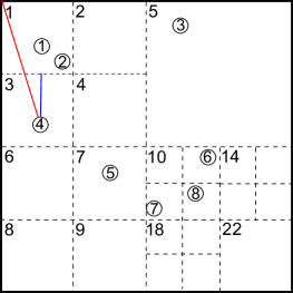
Figure 1: Computing rank bounds

Here, we assume that the space has been partitioned into cells (the space partitioning step is explained in Section 5.1). The rank bound for an object $o$ w.r.t. a cell $c_{q}$ is computed as follows. For any query $q$ arriving with a location in cell $c_{q}$, the rank of $o$ satisfies the condition, ${\bm{r^{\,\downarrow}}}(o,c_{q})\leq{\bm{r}}(o,q)\leq{\bm{r^{\,\uparrow}}}(o,c_{q})$, where ${\bm{r^{\,\downarrow}}}(o,c_{q})$ and ${\bm{r^{\,\uparrow}}}(o,c_{q})$ are the lower and the upper bound rank of $o$ for any query $q$ in cell $c_{q}$, respectively.

Lower rank bound

The lower rank bound, ${\bm{r^{\,\downarrow}}}(o,c_{q})$, is computed such that the rank of object $o$ will be at least ${\bm{r^{\,\downarrow}}}(o,c_{q})$ for a query $q$ contained in cell $c_{q}$. Note that a smaller value of rank indicates a smaller Euclidean distance from the query location. The lower bound rank is computed from the number of objects $o{{}^{\prime}}\in O\backslash o$ that are definitely closer to $q$ in $c_{q}$ than $o$. Specifically, let $\ell_{n}$ be the number of objects $o{{}^{\prime}}\in O\backslash o$ such that ${\bm{d^{\,\uparrow}}}(o{{}^{\prime}},c_{q})\leq{\bm{d^{\,\downarrow}}}(o,c_{q})$, where ${\bm{d^{\,\uparrow}}}(o{{}^{\prime}},c_{q})$ is the maximum Euclidean distance between $o^{\prime}$ and cell $c_{q}$, and ${\bm{d^{\,\downarrow}}}(o,c_{q})$ is the minimum Euclidean distance between $o$ and $c_{q}$. Therefore, even if a query $q$ has a location that is the closest point of $c_{q}$ to $o$, there are still at least $\ell_{n}$ objects closer to $q$ than $o$. So the rank of $o$ must be greater than $\ell_{n}$ for any query in $c_{q}$, meaning that ${\bm{r^{\,\downarrow}}}(o,c_{q})=\ell_{n}+1$. We now give an example of computing the lower rank bound using Figure 1.

Example 1.

Let $O=\{o_{1},o_{2},\dots,o_{8}\}$ be the set of objects and $c_{1}$ be a cell in Euclidean space $X^{d}$. The minimum distance between $c_{1}$ and object $o_{4}$ is shown as the blue line. From Figure 1, only the maximum distance between $c_{1}$ and the object $o_{1}$ is less than ${\bm{d^{\,\downarrow}}}(o_{4},c_{1})$. Therefore, the lower bound rank of $o_{4}$ for cell $c_{1}$ is ${\bm{r^{\,\downarrow}}}$$(o_{4},c_{1})=1+1=2$, i.e., the rank of $o_{4}$ for any query appearing in $c_{1}$ must be greater than or equal to $2$.

Upper rank bound

The upper rank bound ${\bm{r^{\,\uparrow}}}(o,c_{q})$ is the maximum rank an object $o$ can have for any query $q$ appearing in any location of $c_{q}$. This bound is computed as the number of objects that can be closer to $q$ in $c_{q}$ than $o$. Let, $u_{n}$ be the number of objects $o{{}^{\prime}}\in O\backslash o$ such that, ${\bm{d^{\,\downarrow}}}(o{{}^{\prime}},c_{q})<{\bm{d^{\,\uparrow}}}(o,c_{q})$ for any query $q$ in $c_{q}$, where ${\bm{d^{\,\downarrow}}}(o{{}^{\prime}},c_{q})$ is the minimum distance between $o{{}^{\prime}}$ and $c_{q}$ and ${\bm{d^{\,\uparrow}}}(o,c_{q})$ is the maximum distance between $o$ and $c_{q}$. Therefore, even if a query $q$ arrives at the farthest location in $c_{q}$ from $o$, there are at most $u_{n}$ objects that can possibly be closer to $q$ than $o$. So the rank of $o$ cannot be greater than $u_{n}+1$ for any query in $c_{q}$, resulting in ${\bm{r^{\,\uparrow}}}(o,c_{q})=u_{n}+1$.

Example 2.

In Figure 1, the maximum distance from $o_{4}$ to cell $c_{1}$ is shown with a red line. Here, the minimum distance between $c_{1}$ and each of the objects $o_{1},o_{2}$ and $o_{3}$ is less than ${\bm{d^{\,\uparrow}}}(o_{4},c_{1})$. So, ${\bm{r^{\,\uparrow}}}$$(o_{4},c_{1})=3+1=4$. Therefore, the rank of $o_{4}$ for any query in $c_{1}$ must be less than or equal to $4$.

4.2 Indexing Rank

Figure 2: An example inverted rank file

We present an indexing technique called an Inverted Rank File (IRF) where $X^{d}$ is partitioned into different cells, and the rank bounds of each object for queries appearing in the cell is precomputed. The rank information is indexed such that, if a query $q$ arrives anywhere inside a cell $c_{q}$, the rank of any object for $q$ can be estimated. A quadtree structure is employed to partition $X^{d}$ into cells.

First, we present the general structure of an IRF. Later in Section 5.1 we present a space partitioning approach to approximately answer T$m\rho$Q with a guaranteed error bound, and present the rationale behind using a quadtree for space partitioning.

Inverted Rank File

An inverted rank file consists of two components, a collection of all leaf level cells of the quadtree, and a set of rank lists, one for each leaf level cell $c$ of the quadtree. Each rank list is a sorted sequence of tuples of the form $\langle o,{\bm{r^{\,\downarrow}}}(o,c_{q})\rangle$, one for each object $o\in O$, sorted in ascending order of ${\bm{r^{\,\downarrow}}}(o,c_{q})$. If multiple objects have the same ${\bm{r^{\,\downarrow}}}(o,c_{q})$ for a cell $c_{q}$, those tuples are sorted by ${\bm{d^{\,\downarrow}}}(o,c_{q})$. Here, ${\bm{r^{\,\downarrow}}}(o,c_{q})$ is the lower bound rank of $o$ for a query $q$ coming in cell $c_{q}$. Note that, for any object $o$, ${\bm{r^{\,\downarrow}}}(o,c_{q})\leq{\bm{r}}(o,q)$ holds for any query $q$ arriving in any location of $c_{q}$. Each rank list is stored as a sequence of blocks of a fixed length, $B$. Each block $b$ of the rank list for cell $c_{q}$ is associated with the minimum distance between $c_{q}$ and any object in $b$, where ${\bm{d^{\,\downarrow}}}(b,c_{q})=\min_{o\in b}{\bm{d^{\,\downarrow}}}(o,c_{q})$.

Example 3.

Figure 3 illustrates an IRF index for the objects $O=\{o_{1},o_{2},\dots,o_{8}\}$ shown in Figure 1. Assume that the quadtree partitions the space into $22$ disjoint leaf cells as shown in Figure 1, and the size of each block is $B=2$. As a specific example, the lower bound rank of the object $o_{4}$ is $2$ for the quadtree cell $c_{1}$. If a new query arrives in any location contained within cell $c_{1}$, the lower bound of the rank of $o_{4}$ is $2$.

5 Approximate Solution

As the rate of incoming queries can be very high, there may be instances where the cost of computing the exact solution is too expensive. In this section, an approximate solution for the T$m\rho$Q problem is presented. This can be accomplished by using the rank bounds to create an approximate solution with a guaranteed error bound. At the highest level, the approximate solution consists of the following steps:

1. A space partitioning technique is used to construct an IRF index in order to support the incremental computation of the approximate solution of T$m\rho$Q.

2. A safe rank is computed which represents a threshold, if this threshold is exceeded by a result object currently in $\mathscr{R}$, that object must remain in $\mathscr{R}$ as a valid result. Specifically, the current safe rank can be computed by combining: (i) a block based safe rank; and (ii) an object based safe rank.

3. If the ranks of all the result objects are safe, $\mathscr{R}$ does not need to be updated. Otherwise, more work must be done to determine if any object can affect $\mathscr{R}$. This can be achieved using a second technique called validation objects, which incrementally identifies the objects than can affect $\mathscr{R}$. As long as the current result objects have a higher popularity than the validation objects, $\mathscr{R}$ does not need to be updated.

4. If $\mathscr{R}$ must be updated, the approximate popularity of the affected objects are computed. We show that the popularity computations of the prior windows can be used to efficiently approximate the popularity scores of the objects that must change.

We first present the space partitioning approach used to construct the IRF for approximate results in Section 5.1. Then, we present the approximate popularity measure of an object using rank bounding in Section 5.2. In particular, we first outline the workflow of our approximation algorithm, then we propose the notion of safe ranking to determine whether the current result is still valid or not (in Section 5.3), and the notion of validation objects which limit the number of objects to update in the result whenever the window shifts (in Section 5.4). Finally, in Section 5.5 we discuss the error bound guarantees provided by our approximation algorithm.

5.1 Space partitioning

Ideally, rank bound estimations should be as close as possible to the actual rank of each object. If the quadtree leaf cell where a query $q$ arrives is as small as a single point location (i.e., the same as the location of $q$), then both the upper and the lower bound ranks of any object will be exactly the same as the actual rank of that object for $q$. However, if the space is partitioned in this way, then each point in $X^{d}$ will become a leaf cell of the quadtree, and the number of cells will be infinite. Therefore, we propose a partitioning technique which guarantees that the difference between the rank bounds of any object and its true rank is bounded by a threshold, $\epsilon$.

Specifically, for any $o\in O$, and any leaf level cell $c$ of the quadtree, the difference between the upper and the lower bound rank must be within a percentage of the lower bound rank:

$${\bm{r^{\,\uparrow}}}(o,c)-{\bm{r^{\,\downarrow}}}(o,c)\leq\epsilon\times{\bm{r^{\,\downarrow}}}(o,c)$$ (1)

Otherwise, cell $c$ is further partitioned until the condition holds. As an example, let the threshold be $50\%$ of the lower bound, $\epsilon=0.5$. For an object $o$, and a cell $c_{i}$, let ${\bm{r^{\,\downarrow}}}(o,c_{i})=10$ and ${\bm{r^{\,\uparrow}}}(o,c_{i})=20$. So, the cell $c_{i}$ needs to be further partitioned for $o$ until the condition is met. As another example, for the same object $o$ and another cell $c_{j}$, let ${\bm{r^{\,\downarrow}}}(o,c_{j})=100$ and ${\bm{r^{\,\uparrow}}}(o,c_{j})=120$. Now cell $c_{j}$ does not need to be partitioned for $o$ since $120-100\leq 0.5\times 100$.

The intuition behind this partitioning scheme becomes quite clear when the notion of “top” ranked objects is taken into consideration. Getting the exact position of the highest ranked object matters much more than getting the exact position of the object at the thousandth position. So, the granularity of exactness in our inequality degrades gracefully with the true rank of the object.

0.1 Initialize Quadtree with the $X^{d}$

0.2 node $\leftarrow$ Quadtree(root)

0.3 Quadtree(root) $\leftarrow$ Partition(node, $O,\epsilon$)

0.4 return Quadtree

0.5

0.6 Procedure Partition(node,$O,\epsilon$)

0.7 $O^{\prime}$ $\leftarrow\varnothing$

0.8 for $o\in O$ do

0.9       if ${\bm{r^{\,\uparrow}}}(o,\mbox{node})-{\bm{r^{\,\downarrow}}}(o,\mbox{node})>\epsilon\times{\bm{r^{\,\downarrow}}}(o,\mbox{node})$ then

0.10             $O^{\prime}\leftarrow o$

0.11            

0.12      

0.13if $O^{\prime}\neq\varnothing$ then

0.14       Split(node)

0.15       for child of node do

0.16             child $\leftarrow$ Partition(child, $O^{\prime},\epsilon$)

0.17            

0.18 return node

end procedure

Algorithm 1 Quadtree Partition($O,\epsilon$)

Partitioning process

The partitioning of $X^{d}$ using this strategy can be achieved iteratively. Algorithm 1 illustrates the partitioning process. The root of the quadtree is initialized with the entire space $X^{d}$. The process starts from the root cell and recursively partitions $X^{d}$. If the partitioning condition is not satisfied for an object $o$ and a cell $c$, partitioning of $c$ continues until Condition (1) is met (Lines 1.8 - 1.14). The process terminates when for each object $o$, the partitioning condition holds for all of the current leaf level quadtree cells $c$.

Why use a Quadtree? We use a quadtree to partition the space and then organize the spatial information for each quadtree cell. The rationale for using a quadtree is as follows: (i) The quadtree partitions the space into mutually-exclusive cells. In contrast, MBRs in an R-tree may have overlaps, so a query location can overlap with multiple partitions, making it difficult to estimate the object ranks in new queries. (ii) A quadtree is an update-friendly structure, and the partitioning granularity can be dynamically changed using $\epsilon$ to improve the accuracy bounds. This allows performance to be quickly and easily tuned for different collections. (iii) In a quadtree, a cell $c$ is partitioned only when any rank bounds for $c$ do not satisfy Condition (1). In contrast, if a regular grid structure of equal cell size is used, enforcing partitioning using Condition (1) will result in unnecessary cells being created.

Now we present the approximate popularity measure for an object in a sliding window $W$ of queries using the new rank bounds.

5.2 Framework of approximate solution

In this section, we first introduce how to compute the approximate popularity of an object for a given sliding window, then we show how to aggregate the top-$m$ approximate results. Since this section is all about how to compute the approximate popularity of objects, we use the terms popularity and approximate popularity interchangeable, unless specified otherwise.

First, a lemma is presented to show that the rank of any object $o$ for a query $q$ arriving in a cell $c$ can be estimated using only the lower bound rank, ${\bm{r^{\,\downarrow}}}(o,c)$ within an error bound.

Lemma 1.

For any object $o\in O$, and any query $q$ arriving in cell $c$, ${\bm{r^{\,\downarrow}}}(o,c)\leq{\bm{r}}(o,q)\leq(1+\epsilon)\times{\bm{r^{\,\downarrow}}}(o,c)$ always holds.

Proof.

The rank bounds are computed such that ${\bm{r^{\,\downarrow}}}(o,c)\leq{\bm{r}}(o,q)\leq{\bm{r^{\,\uparrow}}}(o,c)$ always holds. For any object $o\in O$, and for any leaf level cell $c$ of the quadtree, the space is partitioned in a way that guarantees ${\bm{r^{\,\uparrow}}}(o,c)-{\bm{r^{\,\downarrow}}}(o,c)\leq\epsilon\times{\bm{r^{\,\downarrow}}}(o,c)$, so, clearly ${\bm{r^{\,\downarrow}}}(o,c)\leq{\bm{r}}(o,q)\leq(1+\epsilon)\times{\bm{r^{\,\downarrow}}}(o,c)$ also holds. ∎

Based on Lemma 1, we approximate the rank of an object with an error bound as:

$${\bm{\hat{r}}}(o,q)=(1+\frac{\displaystyle\epsilon}{\displaystyle 2})\times{\bm{r^{\,\downarrow}}}(o,c)$$ (2)

Corollary 1.

For any object $o\in O$, and any query $q$ arriving in cell $c$, $|{\bm{r}}(o,q)-{\bm{\hat{r}}}(o,q)|\leq\epsilon/2\times{\bm{r^{\,\downarrow}}}(o,c)$ always holds.

Proof.

Here, $\epsilon/2\times{\bm{r^{\,\downarrow}}}(o,c)$ is the average of ${\bm{r^{\,\downarrow}}}(o,c)$ and $(1+\epsilon)\times{\bm{r^{\,\downarrow}}}(o,c)$. Therefore, the proof follows from Lemma 1. ∎

The approximate popularity ${\bm{\hat{\rho}}}(o,W)$ of an object $o$ for the queries $q$ in a $W$ can be computed using rank approximation as:

$${\bm{\hat{\rho}}}(o,W)=\frac{{\sum_{i=1}^{|W|}}\left\{\begin{array}[]{ll}N-{\bm{\hat{r}}}(o,q_{i})+1&\mbox{where }o\in O^{+}_{q_{i}}\\ 0&\mbox{otherwise}\\ \end{array}\right.}{|W|}$$ (3)

Next we present the algorithm to compute the top-$m$ objects with the highest approximate popularity in the sliding window. Later in Section 5.5, we show how to bound the approximation error.

Updating a count based sliding window $W_{i}$ of queries from the previous window $W_{i-1}$ can be formulated as replacing the least recent query $qo$ by the most recent query $qn$ when the sliding window shifts. As a result, only the leaf level cells (in the quadtree) that contain $qn$ and $qo$ need to be found, namely $c_{qn}$ and $c_{qo}$. The rank lists corresponding to these cells can be quickly retrieved from the IRF index. For each window $W_{i}$, assume that $m+1$ objects with the highest ${\bm{\hat{\rho}}}$ are computed, where the top $m$ objects are returned as the result $\mathscr{R}_{i}$ of T$m\rho$Q for $W_{i}$, and the popularity of the $\mathnormal{(m+1)}\cdot$th object is used in the next window to identify the safe rank and the validation objects efficiently.

0.1 Input:

0.2    Window $W_{i}$, number of result objects $m$, the result objects $\mathscr{R}_{i-1}$ of

0.3    the previous window $W_{i-1}$, and the $\mathnormal{m+1}\cdot$th best popularity

0.4    ${\bm{\hat{\rho}}}(o_{m+1},W_{i-1})$ of the previous window $W_{i-1}$.

0.5 Output:  Result objects $\mathscr{R}_{i}$ of the current window $W_{i}$.

0.6 Initialize a max-priority queue $PQ$

0.7 $\mathscr{R}_{i}\leftarrow\emptyset$

0.8 $qn\leftarrow W_{i}\backslash W_{i-1}$

0.9 $qo\leftarrow W_{i-1}\backslash W_{i}$

0.10 for $o\in\mathscr{R}_{i-1}$ do

0.11       ${\bm{\hat{\rho}}}(o,W_{i-1}\backslash qo)\leftarrow{\bm{\hat{\rho}}}(o,W_{i-1})-\frac{\displaystyle\zeta({\bm{\hat{r}}}(o,qo))}{\displaystyle|W_{i}|}$

0.12${\bm{\hat{\rho}}}(o_{m},W_{i-1}\backslash qo)\leftarrow$ the approximate popularity of top $\mathnormal{m}\cdot$th object from $\mathscr{R}_{i-1}$ after updating for $qo$.

0.13

0.14$\mbox{\emph{BSR}}\leftarrow$ Block_safe_rank(${\bm{\hat{\rho}}}(o_{m+1},W_{i-1})$,${\bm{\hat{\rho}}}(o_{m},W_{i-1}\backslash qo)$,$PQ$)

0.15 for $o\in\mathscr{R}_{i-1}$ do

0.16       ${\bm{\hat{\rho}}}(o,W_{i})\leftarrow{\bm{\hat{\rho}}}(o,W_{i-1}\backslash qo)+\frac{\displaystyle\zeta({\bm{\hat{r}}}(o,qn))}{\displaystyle|W|}$

0.17       if ${\bm{\hat{r}}}(o,qn)\leq\mbox{BSR}$ and $o\in O^{+}_{qn}$ then

0.18             $\mathscr{R}_{i}\leftarrow o$

0.19      

0.20if $|\mathscr{R}_{i}|<m$ then

0.21       ${\bm{\hat{\rho}}}(o_{m},W_{i})\leftarrow$ current $\mathnormal{m}\cdot$th best popularity of $\mathscr{R}_{i-1}$ in $W_{i}$.

0.22       $\mbox{\emph{OSR}}\leftarrow$ Object_safe_rank(${\bm{\hat{\rho}}}(o_{m+1},W_{i-1}),{\bm{\hat{\rho}}}(o_{m},W_{i}),PQ$)

0.23       for $o\in\mathscr{R}_{i-1}\backslash\mathscr{R}_{i}$ do

0.24             if ${\bm{\hat{r}}}(o,qn)\leq\mbox{OSR}$ and $o\in O^{+}_{qn}$ then

0.25                   $\mathscr{R}_{i}\leftarrow o$

0.26            

0.27

0.28if $|\mathscr{R}_{i}|<m$ then

0.29       VO $\leftarrow$ Validation_objects(${\bm{\hat{\rho}}}(o_{m},W_{i})$, $PQ$)

0.30       if VO $\neq\emptyset$ then

0.31             $\mathscr{R}_{i}$ $\leftarrow$ Update_results($\mbox{\emph{VO}},\mathscr{R}_{i-1}\backslash\mathscr{R}_{i}$)

0.32            

0.33      

0.34

return $\mathscr{R}_{i}$

Algorithm 2 T$m\rho$Q

The steps for updating the approximate solution of T$m\rho$Q for a window $W_{i}$ are shown in Algorithm 2. Note that notation was previously defined in Table 1. Here, $\zeta(o,q)$ is the contribution of $q$ to the popularity of $o$, and is computed as:

$\zeta({\bm{\hat{r}}}(o,q))=\left\{\begin{array}[]{ll}N-{\bm{\hat{r}}}(o,q)+1&\mbox{where }o\in O^{+}_{q}\\ 0&\mbox{otherwise}\\ \end{array}\right.$

First, the approximate popularity of the result objects $o\in\mathscr{R}_{i-1}$ for the excluded query $qo$ with ${\bm{\hat{r}}}(o,qo)$ is updated. Let the updated $\mathnormal{m}\cdot$th highest popularity from the set of $\mathscr{R}_{i-1}$ be ${\bm{\hat{\rho}}}(o_{m},W_{i-1}\backslash qo)$ (Lines 2.10 - 2.12 in Algorithm 2). The rest of the algorithm consists of three main components - (i) computing the safe rank in two steps (block based and object based safe rank), (ii) finding the set of validation objects, and (iii) updating $\mathscr{R}_{i}$.

Locating an object in IRF

Since some of the steps in Algorithm 2 require finding the entry of a particular object in a rank list in IRF, we first present an efficient technique for locating objects, and then describe the remaining steps of the approximation algorithm.

We start with a lemma to find a relation between the minimum Euclidean distance of the objects from a cell $c$ and the lower rank bounds of the objects for any query in cell $c$.

Lemma 2.

For any two objects $o_{i},o_{j}\in O$ and a cell $c$, if ${\bm{r^{\,\downarrow}}}(o_{i},c)\leq{\bm{r^{\,\downarrow}}}(o_{j},c)$, then ${\bm{d^{\,\downarrow}}}(o_{i},c)\leq{\bm{d^{\,\downarrow}}}(o_{j},c)$ always holds.

Proof.

We prove the lemma using proof by contradiction. Assume that ${\bm{d^{\,\downarrow}}}(o_{i},c)>{\bm{d^{\,\downarrow}}}(o_{j},c)$ is true. In the rank list of IRF, the entries $\langle o,{\bm{r^{\,\downarrow}}}(o,c)\rangle$ are sorted in ascending order of the lower rank bound, ${\bm{r^{\,\downarrow}}}(o,c)$. Here, ${\bm{r^{\,\downarrow}}}(o,c)$ is the number of objects $o^{\prime}$ (plus 1) that are guaranteed to be closer to $c$ than $o$. So, ${\bm{d^{\,\uparrow}}}(o^{\prime},c)\leq{\bm{d^{\,\downarrow}}}(o,c)$. Let $\mid O^{\prime}_{i}\mid=\ell_{i}$ be the set of all the objects from $O$ such that $\forall o^{\prime}_{i}\in O^{\prime}_{i}$, ${\bm{d^{\,\uparrow}}}(o^{\prime}_{i},c)\leq{\bm{d^{\,\downarrow}}}(o_{i},c)$, and $\mid O^{\prime}_{j}\mid=\ell_{j}$ be the set of objects where $\forall o^{\prime}_{j}\in O^{\prime}_{j}$, ${\bm{d^{\,\uparrow}}}(o^{\prime}_{j},c)\leq{\bm{d^{\,\downarrow}}}(o_{j},c)$. As ${\bm{r^{\,\downarrow}}}(o_{i},c)\leq{\bm{r^{\,\downarrow}}}(o_{j},c)$, then $\ell_{i}\leq\ell_{j}$ is also true.

Since ${\bm{d^{\,\downarrow}}}(o_{i},c)>{\bm{d^{\,\downarrow}}}(o_{j},c)$ was assumed to be true, ${\bm{d^{\,\uparrow}}}(o^{\prime}_{j},c)\leq{\bm{d^{\,\downarrow}}}(o_{j},c)<{\bm{d^{\,\downarrow}}}(o_{i},c)$. Therefore, $o^{\prime}_{i}$ and $o^{\prime}_{j}$ both are in the set of objects from $O$ that satisfy ${\bm{d^{\,\uparrow}}}(o^{\prime}_{i},c)\leq{\bm{d^{\,\downarrow}}}(o_{i},c)$, and ${\bm{d^{\,\uparrow}}}(o^{\prime}_{j},c)<{\bm{d^{\,\downarrow}}}(o_{i},c)$, respectively. Hence, $O^{\prime}_{j}\subseteq O^{\prime}_{i}$, so $\ell_{j}\leq\ell_{i}$ must be true. But this is a contradiction. Therefore, ${\bm{d^{\,\downarrow}}}(o_{i},c)>{\bm{d^{\,\downarrow}}}(o_{j},c)$ cannot be true. If ${\bm{r^{\,\downarrow}}}(o_{i},c)\leq{\bm{r^{\,\downarrow}}}(o_{j},c)$ is true, ${\bm{d^{\,\downarrow}}}(o_{i},c)\leq{\bm{d^{\,\downarrow}}}(o_{j},c)$ must hold. ∎

Lemma 2 show that sorting the objects by the value of ${\bm{r^{\,\downarrow}}}(o,c)$ is equivalent to sorting the objects by their minimum Euclidean distance to $c$, ${\bm{d^{\,\downarrow}}}(o,c)$. If multiple objects have the same ${\bm{r^{\,\downarrow}}}(o,c)$, they are already stored as sorted by their ${\bm{d^{\,\downarrow}}}(o,c)$ as described in Sec. 4.2. Therefore, we can locate an entry position of object $o$ in the rank list of cell $c$ (in IRF) in three steps.
(1) Compute the minimum Euclidean distance ${\bm{d^{\,\downarrow}}}(o,c)$ of $c$ from $o$.
(2) Using an IRF as described in Sec. 4.2, each block $b$ of the rank list for cell $c$ is associated with the minimum distance between $c_{q}$ and any object in $b$, ${\bm{d^{\,\downarrow}}}(b,c)$, so a binary search on ${\bm{d^{\,\downarrow}}}(b,c)$ can be performed to find the position of the block $b$ where $o$ is stored.
(3) Perform a linear scan in that block to find the entry for $o$.

The entire process has $\mathscr{O}(log_{2}(N/B)+B)$ time complexity, where $B$ is the number of objects in a block.

5.3 Safe rank

Recall that in Algorithm 2 the purpose of finding a safe rank is to minimize the number of updates in $\mathscr{R}_{i-1}$ (result objects in the previous window $W_{i-1}$) to get the result set $\mathscr{R}_{i}$ (in the current window $W_{i}$) whenever the sliding window shifts. In particular, the idea is to compute the safe rank OSR for the objects $o\in\mathscr{R}_{i-1}$ such that, if ${\bm{\hat{r}}}(o,qn)<\mbox{\emph{OSR}}$, then no other object from $o^{\prime}\in O\backslash\mathscr{R}_{i-1}$ can have a higher ${\bm{\hat{\rho}}}$ than $o$, thereby $o$ is a valid result in $\mathscr{R}_{i}$ as well. Note that a smaller value of rank implies a higher contribution in the popularity measure. The safe rank is defined w.r.t. the current window $W_{i}$ by default.

Before presenting the computation of an object’s safe rank, the concept of popularity gain of an object $o$ is introduced, which results from replacing the least recent query $qo$ by the most recent query $qn$, and is denoted by $\Delta_{o}$:

$$\Delta_{o}={\bm{\hat{\rho}}}(o,W_{i})-{\bm{\hat{\rho}}}(o,W_{i-1})=\frac{\zeta({\bm{\hat{r}}}(o,qn))-\zeta({\bm{\hat{r}}}(o,qo))}{|W_{i}|}$$ (4)

Here, if $o$ does not satisfy the query constraint ${\mbox{\em Con}}(q)$, the contribution of $q$ to the popularity of $o$, $\zeta({\bm{\hat{r}}}(o,qn))=0$.

Let $\Delta_{o}^{\,\uparrow}$ denote the maximum popularity gain among all objects (in the current window $W_{i}$). Then the popularity of any object $o^{\prime}\in O\backslash\mathscr{R}_{i-1}$ can be at most ${\bm{\hat{\rho}}}(o_{m+1},W_{i-1})+\Delta_{o}^{\,\uparrow}$, where ${\bm{\hat{\rho}}}(o_{m+1},W_{i-1})$ is the $\mathnormal{(m+1)}\cdot$th highest approximate popularity in the previous window $W_{i-1}$. In other words, if the updated popularity of an object $o\in\mathscr{R}_{i-1}$ is higher (better) than ${\bm{\hat{\rho}}}(o_{m+1},W_{i-1})+\Delta_{o}^{\,\uparrow}$, then such an $o$ is guaranteed to remain in $\mathscr{R}_{i}$, which inspires the design of the object-level safe rank OSR shown in the following equation:

$${\bm{\hat{\rho}}}(o_{m},W_{i-1}\backslash qo)+\frac{N-\mbox{\emph{OSR}}+1}{|W_{i}|}\geq{\bm{\hat{\rho}}}(o_{m+1},W_{i-1})+\Delta_{o}^{\,\uparrow}$$ (5)

Since a lower rank indicates a higher contribution to the popularity, the gain will be maximized when the difference between $\zeta({\bm{\hat{r}}}(o,qn))$ and $\zeta({\bm{\hat{r}}}(o,qo))$ is maximized. Therefore, the goal of minimizing the updates of objects in $R_{i-1}$ (set at the beginning of this section) can be reduced to the challenge of how to compute a tight estimation of $\Delta_{o}^{\,\uparrow}$.

A naive approach to estimate $\Delta_{o}^{\,\uparrow}$ is to overestimate $\zeta({\bm{\hat{r}}}(o,qn))$ as $N-1+1$ (the rank of $o$ is “1” for $qn$) and underestimate $\zeta({\bm{\hat{r}}}(o,qo))$ as “0” ($o$ does not satisfy ${\mbox{\em Con}}(qo)$). The safe rank OSR for $W_{i}$ can then be computed using the naive maximum gain value in Eqn. 5. However, such an estimation of the maximum gain is too loose, and may not have any pruning capacity, especially if the queries $qn$ and $qo$ are close to each other (an object that is ranked very high for $qn$ but ranked very low for $qo$ may not exist).

5.3.1 Block-level popularity gain

Since the objects are arranged blockwise in an IRF index, and each object $o$ is sorted by its lower bound rank ${\bm{r^{\,\downarrow}}}(o,c_{q})$ in ascending order, we are motivated to define and utilize a block-level gain as the first step in finding a tighter estimation of the maximum object-level gain.

In particular, a block-level maximum gain $\Delta_{b}^{\,\uparrow}$ is computed, such that $\Delta_{b}^{\,\uparrow}\geq\Delta_{o}^{\,\uparrow}$, which can be used to find the block-level safe rank, BSR. If the rank of any result object is not better than BSR for $qn$, then an object-level maximum gain, $\Delta_{o}^{\,\uparrow}$ is computed. The object-level safe rank OSR can be computed using this value, where $\mbox{\emph{OSR}}\geq\mbox{\emph{BSR}}$, as a lower value of rank implies a higher gain. If the rank of any result object is still not safe, then the validation objects (proposed in Sec. 5.4) must be checked to decide if $\mathscr{R}_{i-1}$ needs to be updated. Here, some part of the safe rank calculations can be reused to find the validation objects, which will be explained in Section 5.4.

Next, we define the block-level gain and propose a technique to compute the block-level maximum gain, from which a block-level safe rank BSR can be computed in the following section.

Block-level gain computation

Figure 3: Upper bound rank computation of a block

Given a block $b$ from the rank list of $qn$, the block-level gain $\Delta_{b}$ is an overestimation of the gain of the objects $o\in b$, such that $\Delta_{b}\geq\Delta_{o}$. As the gain is maximized when the difference between $\zeta({\bm{\hat{r}}}(o,qn))$ and $\zeta({\bm{\hat{r}}}(o,qo))$ is maximized, a technique to compute $\Delta_{b}$ can be actualized by finding: (i) a lower bound estimation of the rank of any object $o\in b$ for $qn$, namely ${\bm{\hat{r}^{\,\downarrow}}}(b,qn)$, where, ${\bm{\hat{r}^{\,\downarrow}}}(b,qn)\leq{\bm{\hat{r}}}(o,qn)$; and (ii) an upper bound estimation of the rank that any object $o\in b$ can have for $qo$, denoted as ${\bm{\hat{r}^{\,\uparrow}}}(b,qo)$, such that ${\bm{\hat{r}}}(o,qo)\leq{\bm{\hat{r}^{\,\uparrow}}}(b,qo)$.

Since the objects are sorted in ascending order of lower bound ranks in the IRF index, the lower bound rank of the first entry of $b$ is implicitly ${\bm{\hat{r}^{\,\downarrow}}}(b,qn)$. Here, $\forall o\in b,{\bm{\hat{r}^{\,\downarrow}}}(b,qn)\leq{\bm{r^{\,\downarrow}}}(o,qn)$ holds by definition.

Next, for the same block $b$ of the rank list of $qn$, finding the maximum rank ${\bm{\hat{r}^{\,\uparrow}}}(b,qo)$ that any object $o\in b$ can have for $qo$ is needed. To achieve this, a block $b^{\prime}$ is found such that all of the objects $o\in b$ are guaranteed to be in the rank list of $qo$ before $b^{\prime}$. As the objects are sorted by ${\bm{r^{\,\downarrow}}}(o,c_{qo})$ in the rank list of $c_{qo}$, ${\bm{r^{\,\downarrow}}}(o^{\prime},c_{qo})$ is guaranteed to be greater than that of any object in $b^{\prime}$, where $o^{\prime}$ is the first entry of $b^{\prime}$. Therefore, ${\bm{r^{\,\downarrow}}}(o^{\prime},qo)$ is taken as the upper bound estimation, ${\bm{\hat{r}^{\,\uparrow}}}(b,qo)$.

For a tight estimation of ${\bm{\hat{r}^{\,\uparrow}}}(b,qo)$, the block $b^{\prime}$ with the smallest ${\bm{r^{\,\downarrow}}}(o^{\prime},qo)$ must be found. As the objects and blocks of a rank list are sorted by the minimum Euclidean distance from the corresponding cell (Section 4.2), and $\forall o\in b,$ ${\bm{d^{\,\downarrow}}}(o,c_{qo})\leq{\bm{d^{\,\uparrow}}}(b,c_{qo})$, a binary search over the blocks of the rank list of $qo$ is performed to find the first position of the block $b^{\prime}$ where ${\bm{d^{\,\uparrow}}}(b,c_{qo})\leq{\bm{d^{\,\downarrow}}}(b^{\prime},c_{qo})$. Here, ${\bm{d^{\,\uparrow}}}(b,c_{qo})$ is computed as the maximum Euclidean distance between the minimum bounding rectangle of the objects $o\in b$ and cell $c_{qo}$.

Example 4.

Computing the block gain is explained with the example in Figure 3. Let $c_{1}$ and $c_{2}$ be the cell where query $qn$ and $qo$ arrive respectively. Assume that the constraint of both queries are satisfied by all the objects for ease of explanation. Let $b=\langle(o_{4},2),(o_{5},4)\rangle$ be the block of the rank list of $qn$ currently under consideration. Here, ${\bm{\hat{r}^{\,\downarrow}}}(b,qn)=2$, which is the lower bound of the first entry of $b$. Let ${\bm{d^{\,\uparrow}}}(b,c_{2})=14$, computed from the MBR of block $b$ and cell $c_{2}$. Now, as the objects and the blocks in the rank list of $c_{2}$ are sorted by their minimum Euclidean distance from $c_{2}$, a binary search is performed with the value $14$ over the ${\bm{d^{\,\downarrow}}}$ of the blocks in $c_{2}$. Note that, $b$ is a block in the rank list of $c_{1}$, consisting of the objects $o_{4}$ and $o_{5}$. Here, we get $b^{\prime}=\langle(o_{6},6),(o_{8},6)\rangle$, as ${\bm{d^{\,\downarrow}}}(b^{\prime},c_{2})=18$, which is the smallest value of ${\bm{d^{\,\downarrow}}}$ greater than $14$, shown with an arrow. So, ${\bm{\hat{r}^{\,\uparrow}}}(b,qo)=6$ is the lower bound rank of the first entry of $b^{\prime}$.

5.3.2 Block-level safe rank

0.1 Input:

0.2    ${\bm{\hat{\rho}}}(o_{m+1},W_{i-1})$ - $\mathnormal{(m+1)}\cdot$th highest popularity of $W_{i-1}$,

0.3    ${\bm{\hat{\rho}}}(o_{m},W_{i-1}\backslash qo)$ - $\mathnormal{m}\cdot$th highest popularity from $\mathscr{R}_{i-1}$ after updating

0.4    for $qo$, and $PQ$ - a max-priority queue.

0.5 Output:  Block based safe rank - BSR

0.6 $b\leftarrow$ first block in the rank list of $c_{qn}$.

0.7 $\Delta_{b}^{\,\uparrow}\leftarrow 0$

0.8 do

0.9       ${\bm{\hat{r}^{\,\downarrow}}}(b,qn)\leftarrow{\bm{r^{\,\downarrow}}}(o,c_{qn})$ of the first entry $o$ from $b$.

0.10       ${\bm{d^{\,\uparrow}}}(b,c_{qo})\leftarrow$ Maximum Euclidean distance between $b$ and $c_{qo}$.

0.11       $b^{\prime}\leftarrow$ First position of the block of $c_{qo}$, where ${\bm{d^{\,\uparrow}}}(b,c_{qo})\leq{\bm{d^{\,\downarrow}}}(b^{\prime},c_{qo})$.

0.12       ${\bm{\hat{r}^{\,\uparrow}}}(b,qo)\leftarrow$ ${\bm{r^{\,\downarrow}}}(o^{\prime},c_{qo})$ of the first entry $o^{\prime}$ of $b^{\prime}$.

0.13       $\Delta_{b}\leftarrow\frac{\displaystyle\zeta({\bm{\hat{r}^{\,\downarrow}}}(b,qn))-\zeta(\displaystyle{\bm{\hat{r}^{\,\uparrow}}}(b,qo))}{\displaystyle|W|}$

0.14       Enqueue ($PQ,b,\Delta_{b})$

0.15       $\Delta_{b}^{\,\uparrow}\leftarrow\Delta_{top(PQ)}$

0.16       $b\leftarrow$ Next ($c_{qn}$)

0.17      

0.18while $b$ cannot have a better gain than $\Delta_{b}^{\,\uparrow}$;

0.19BSR $\leftarrow$ Compute from ${\bm{\hat{\rho}}}(o_{m+1},W_{i-1})$,${\bm{\hat{\rho}}}(o_{m},W_{i-1}\backslash qo)$, $\Delta_{b}^{\,\uparrow}$ as Eqn. 6.

return BSR

Algorithm 3 Block_safe_rank

By making use of the values ${\bm{\hat{r}^{\,\downarrow}}}(b,qn)$ and ${\bm{\hat{r}^{\,\uparrow}}}(b,qo)$ of block $b$, a block-level estimation of the maximum gain for $W_{i}$ can found, and a block-level safe rank BSR can be computed, as shown in Algorithm 3. Algorithm 3 shows the steps needed to compute the block-level safe rank by finding the maximum gain of a block using the rank lists of $qn$ and $qo$. A max-priority queue PQ is used to keep track of blocks that must be visited, where the key is $\Delta_{b}$. Here, $\Delta_{b}$ is an overestimation of the gain of the objects in $b$. For any object $o\in b$, $\Delta_{o}\leq\Delta_{b}$, is computed in Line 3.13 as -

$$\Delta_{b}\leftarrow\frac{\displaystyle\zeta({\bm{\hat{r}^{\,\downarrow}}}(b,qn))-\zeta(\displaystyle{\bm{\hat{r}^{\,\uparrow}}}(b,qo))}{\displaystyle|W_{i}|}$$

Recall that in the IRF index, each object $o$ in the rank list is sorted in ascending order of the lower bound rank w.r.t. the cell $c_{qn}$, and the traversal starts from the beginning of the rank list of $c_{qn}$ so that the objects with a higher gain are most likely to be explored first. The traversal continues until the subsequent blocks of the rank lists of $qn$ cannot have a better gain than the current maximum gain $\Delta_{b}^{\,\uparrow}$ found so far. Here, the terminating condition of Line 3.17 is:

$$\frac{\zeta({\bm{\hat{r}^{\,\downarrow}}}(b,qn))}{|W_{i}|}<\Delta_{b}^{\,\uparrow}$$

Lastly, in Line 3.18 the maximum gain value $\Delta_{b}^{\,\uparrow}$ is used to compute the block-level safe rank as follows:

$${\bm{\hat{\rho}}}(o_{m},W_{i-1}\backslash qo)+\frac{N-\mbox{\emph{BSR}}+1}{|W_{i}|}\geq{\bm{\hat{\rho}}}(o_{m+1},W_{i-1})+\Delta_{b}^{\,\uparrow}$$ (6)

5.3.3 Object-level safe rank

0.1 Input:

0.2    ${\bm{\hat{\rho}}}(o_{m+1},W_{i-1})$ - $\mathnormal{(m+1)}\cdot$th highest popularity of $W_{i-1}$,

0.3    ${\bm{\hat{\rho}}}(o_{m},W_{i-1}\backslash qo)$ - the updated $\mathnormal{m}\cdot$th highest popularity from $\mathscr{R}_{i-1}$

0.4    after removing $qo$, and $PQ$ - a max-priority queue from    Block_safe_rank.

0.5 Output:  Object-level safe rank, OSR

0.6 while $PQ$ not empty do

0.7       $E\leftarrow$ Dequeue ($PQ$)

0.8       if E is object then

0.9             $\Delta_{o}^{\,\uparrow}\leftarrow\Delta_{E}$

0.10             break

0.11            

0.12       else

0.13             for o in E do

0.14                   $\Delta_{o}\leftarrow\frac{\displaystyle\zeta({\bm{\hat{r}}}(o,qn))-\zeta({\bm{\hat{r}}}(o,qo))}{\displaystyle|W|}$

0.15                   Enqueue ($PQ,o,\Delta_{o}$)

0.16                  

0.17OSR $\leftarrow$ Compute from ${\bm{\hat{\rho}}}(o_{m},W_{i})$,${\bm{\hat{\rho}}}(o_{m},W_{i-1}\backslash qo)$,$\Delta_{o}^{\,\uparrow}$ (by Eqn. 5).

return $OSR$

Algorithm 4 Object_safe_rank

If the rank of any object $o\in\mathscr{R}_{i-1}$ for $qn$ is not smaller (better) than the block-level safe rank BSR, then the object-level safe rank is computed, where $\mbox{\emph{OSR}}\geq\mbox{\emph{BSR}}$ is used to further determine whether the result needs to updated or not (Lines 2.18 - 2.23 in Algorithm 2).

Algorithm 4 shows a best-first approach to compute the maximum object gain using the same priority queue PQ maintained in the block-level computation. In each iteration, the top element $E$ of PQ is dequeued from PQ. If $E$ is a block, the approximate rank of each object $o\in E$ for $qn$ and $qo$ is computed using the corresponding lower bound rank in the rank lists. The objects are then enqueued in PQ, and indexed by the gain computed using Eqn. 4. If $E$ is an object, then the gain is returned as the maximum object level gain $\Delta_{o}^{\,\uparrow}$ (Lines 4.8 - 4.9). The object-level safe rank, OSR, is then computed in the same manner as Eqn. 6 with the value $\Delta_{o}^{\,\uparrow}$.

5.4 Validation objects

If the rank of any object $o\in\mathscr{R}_{i-1}$ is not safe, a set of validation objects VO is found such that, as long as $\forall vo\in\mbox{\emph{VO}}$, ${\bm{\hat{\rho}}}(o,W_{i})\geq{\bm{\hat{\rho}}}(vo,W_{i})$, $o$ is a valid result object of $\mathscr{R}_{i}$. We present an efficient approach to incrementally identify VO. Furthermore, we show that if the result needs to be updated, the new result objects also must come from VO.

First, after a new query $qn$ arrives, the approximate rank for each object $o\in\mathscr{R}_{i-1}$ is computed, and the appropriate popularity scores are updated. Let the updated $\mathnormal{m}\cdot$th highest approximate popularity from $\mathscr{R}_{i-1}$ be ${\bm{\hat{\rho}}}(o_{m},W_{i})$ (Line 2.19 of Algorithm 2). The priority queue PQ maintained for safe rank computation is used to find the set VO of validation objects, where ${\bm{\hat{\rho}}}(o_{m},W_{i})$ is used as a threshold to terminate the search.

A best-first search is performed using PQ to find the objects that have gain high enough to be a result. Specifically, if the dequeued element $E$ from PQ is a block, the ${\bm{\hat{r}}}$ of each object $o$ in $E$ is computed for $qn$ and $qo$ in the same manner as described for the object-level safe rank computation. As the popularity of an object $o\in O\backslash\mathscr{R}_{i-1}$ can be at most ${\bm{\hat{\rho}}}(o_{m+1},W_{i-1})+\Delta_{o}$, an object $o$ is included in the validation set if $o$ satisfies the following condition:

$${\bm{\hat{\rho}}}(o_{m+1},W_{i-1})+\Delta_{o}\geq{\bm{\hat{\rho}}}(o_{m},W_{i})$$ (7)

As PQ is a max-priority queue which is maintained for the gain of the objects and the blocks, the process can be safely terminated when the gain of a dequeued element $E$ does not satisfy the condition in Equation 7.

If no validation object is found, this implies that there is no object that can have a higher popularity than the current results. In this case, the result set $\mathscr{R}_{i-1}$ (of previous window $W_{i-1}$) remains unchanged, and is the result of current window $W_{i}$. Otherwise, the popularity of each object in $\mathscr{R}_{i-1}\backslash\mathscr{R}_{i}$ needs to be checked against the popularity of the validation objects $vo\in\mbox{\emph{VO}}$ to update the result.

5.4.1 Updating results

As described in Section 5.4, the set of validation objects VO is computed such that no object $o\backslash\mbox{\emph{VO}}$ can have a higher popularity than any of the objects in $\mathscr{R}_{i-1}$. Therefore, only objects in VO are considered when updating the result set. To update the results using the objects $vo\in\mbox{\emph{VO}}$, the popularity of $vo$ for the current window must be computed. Therefore, an efficient technique to compute the popularity of the validation objects is now presented.

Computing ${\bm{\hat{\rho}}}$ of the validation objects

As the popularity gain of each $vo\in\mbox{\emph{VO}}$ has already been computed as described in Section 5.4, it is sufficient to find the ${\bm{\hat{\rho}}}(vo,W_{i-1}\backslash qo)$ and use it to compute ${\bm{\hat{\rho}}}(vo,W_{i})$. Since the popularity of every object for every window is not computed, a straightforward way to compute ${\bm{\hat{\rho}}}(vo,W_{i-1}\backslash qo)$ is to find the rank of $vo$ for each $q\in W_{i-1}\backslash qo$ using the corresponding rank lists. However, this approach is computationally expensive, especially when the window size is large. Moreover, if $vo$ was a validation object or a result object in a prior window $W_{i-y}$, then the same computations are repeated unnecessarily for the queries shared by the windows (the queries contained in $W_{i}\cap W_{i-y}$).

Therefore, if ${\bm{\hat{\rho}}}$ of a result or a validation object is computed for a window $W_{i-y}$, the aim is to reuse this computation for later windows in an efficient way. This can be accomplished by storing the popularity of a subset of “necessary” objects from prior windows for later reuse. We show that the choice of these limited number of windows is optimal, and storing the popularity for any additional windows cannot reduce the computational cost any further.

Choosing the limited number of prior windows

The popularity computations can be reused if the number of shared queries among the windows is greater than the number of queries that differ. Otherwise, the popularity must be computed for the window $W_{i}$ from scratch rather than reusing the popularity computations from $W_{i-y}$. Specifically, let $Y$ be the number of shared queries among windows $W_{i}$, $W_{i-y}$ ($Y=|W_{i}\cap W_{i-y}|$), $Q_{o}=W_{i-y}\backslash W_{i}$, and $Q_{n}=W_{i}\backslash W_{i-y}$. So in a count based window, $|Q_{n}|=|W_{i}|-Y$ and $|Q_{o}|=|W_{i}|-Y$, as each time the sliding window shifts, a new query is inserted and the least recent query is removed from the window. If the number of computations required for the shared queries is greater than the number of computations for $|Q_{n}|+|Q_{o}|$, i.e., $Y\geq 2(|W_{i}|-Y)$, then computations can be reused. So the number of shared queries, $Y$, should be greater than or equal to $2|W_{i}|/3$ for efficient reuse.

Reusing popularity computations

If the condition $Y\geq 2|W_{i}|/3$ holds, the popularity of an object $o$ computed for $W_{i-y}$ can be used as ${\bm{\hat{\rho}}}(o,W_{i})$ as follows:

$${\bm{\hat{\rho}}}(o,W_{i})={\bm{\hat{\rho}}}(o,W_{i-y})+$$ (8)

$$\frac{\sum_{qn\in Q_{n}}\zeta({\bm{\hat{r}}}(o,qn))-\sum_{qo\in Q_{o}}\zeta({\bm{\hat{r}}}(o,qo))}{|W_{i}|}$$

Popularity lookup table

A popularity lookup table is maintained with the popularity of the result and validation objects for the most recent $2|W_{i}|/3$ windows. If a validation object $vo$ of the current window $W_{i}$ is found in the lookup table, the popularity is computed using Equation 8. Otherwise, the popularity of $vo$ is computed from the rank lists of the queries in $W_{i}$. The popularity $vo$ for $W_{i}$ is then added to the popularity lookup table for later windows.

Obtaining Results

The objects $vo\in\mbox{\emph{VO}}$ are considered one by one to update the results. After computing the popularity of an object $vo\in\mbox{\emph{VO}}$, if ${\bm{\hat{\rho}}}(vo,W_{i})>{\bm{\hat{\rho}}}(o_{m},W_{i})$, then $vo$ is added to $\mathscr{R}_{i}$. The set $\mathscr{R}_{i}$ is adjusted such that it contains $m$ objects with the highest ${\bm{\hat{\rho}}}$, and the value of ${\bm{\hat{\rho}}}(o_{m},W_{i})$ is adjusted accordingly. In this process, if the overestimated popularity of an object $vo$ computed with Eqn 7 is less than the updated ${\bm{\hat{\rho}}}(o_{m},W_{i})$, that object can be safely discarded from consideration without computing its popularity.

5.5 Approximation error bound

In this section we present the bound for approximation error of our proposed approach. Specifically we show that, for any object $o\in O$, and any window $W$ of queries, the ratio between ${\bm{\hat{\rho}}}(o,W)$ and $\rho(o,W)$ is bounded.

Lemma 3.

For any object $o\in O$, and a window $W$ of queries, the approximation ratio is bounded by $1-\epsilon/2N$.
(i) ${\bm{\hat{\rho}}}(o,W)/\rho(o,W)\leq 1-\epsilon/2N$ when $\rho(o,W)\geq{\bm{\hat{\rho}}}(o,W)$; and
(ii) $\rho(o,W)/{\bm{\hat{\rho}}}(o,W)\leq 1-\epsilon/2N$ when ${\bm{\hat{\rho}}}(o,W)\geq\rho(o,W)$ always holds.

Proof.

See Appendix A ∎

6 Experimental Evaluation

In this section, we present the experimental evaluation for our proposed approach to monitor the top-$m$ popular objects in a sliding window of streaming queries. As there is no prior work that directly answers this problem (Section 2), we compare our approximate solution (proposed in Section 5), denoted by AP, with the baseline exact approach (proposed in Section 3.2), denoted by BS.

6.1 Experiment Settings

Datasets and query generation

All experiments were conducted using two real datasets, (i) Aus dataset at a city scale and (ii) Foursq dataset at a country scale.

The Aus dataset contains $52,913$ real estate properties sold in a major Metropolitan city in Australia between 2013 to 2015, collected from the online real estate advertising site. As a property can be sold multiple times over the period, only the first sale was retained in the dataset. The locations of the queries in the Aus dataset were created by using locations of $987$ facilities (train stations, schools, hospitals, supermarkets, and shopping centers) in this region. We generated two sets of queries from these locations, each of size $20K$. Repeating queries were created using two different approaches: (i) uniform; and (ii) skewed distribution respectively. We denote the uniform and the skewed query set as U and S, respectively. The radius of the queries are varied as an experimental parameter, and is discussed further in Section 6.2.

The Foursq dataset contains $304,133$ points of interest (POI) from Foursquare in $34$ cities spread throughout the USA. The queries for the Foursq dataset were generated using the user check-ins. From the check-ins of each user, we generated a query, where the query location was the centroid of all the check-ins of that user, and the query radius was set as the minimum distance that covers these check-ins. If a user has only one check-in record, we set the query location as the check-in location, and the radius of the query is randomly assigned from another user. As a result, a total of $22,442$ queries were generated for the Foursq dataset.

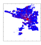
(a) Aus

(b) Foursq

Figure 4: Dataset and query locations

Since Aus dataset represents a real city-level data and queries are real facilities in that city, it is the best candidate for effectiveness study; as a result we conducted efficiency and effectiveness study on Aus. Since the queries generated for Foursq spread over the whole country, we find that it is more suitable for the efficiency and scalability study; nonetheless, we conducted the effectiveness study for Foursq and most experiment results are shown in Appendix B.

After initializing the sliding window, we evaluated the performance of both BS and AP approaches for $10K$ query arrivals in the stream, i.e., $10K$ shifts of the sliding window. We repeated the process $50$ times, and report the mean performance. For the Aus dataset, the arrival order of the queries was randomly generated. For the Foursq dataset, the arrival order of a query in the stream was obtained from the most recent check-in time of the corresponding user. Figure 4 shows the location distribution of the objects, and the queries for both datasets, where the blue and the red points represent object locations and query locations respectively. Note that, for the Foursq dataset, the POIs are clustered in large cities (i.e., blue clusters). As a user may check-in in different cities, the queries (which are the centroid of the check-in locations) are distributed in different locations across the US.

Table 2: Parameters

Parameter	Range
$W$	$100,200,{\bf 400},800,1600$
$m$	$1,5,{\bf 10},20,50,100$
Query radius (%)	$1,2,{\bf 4},8,16$
$\epsilon$	$1,2,{\bf 3},4,5$
$B$	$32,64,{\bf 128},256,512$

Evaluation Metrics & Parameter

We studied the efficiency, scalability and effectiveness for both the baseline approach (BS), and the approximate approach (AP) by varying several parameters. The parameter of interest and their ranges are listed in Table 2, where the values in bold represent the default values. For all experiments, a single parameter varied while keeping the rest as the default settings. For efficiency and scalability, we studied the impact of each parameter on: the number of objects whose popularity are computed per query (OPQ), to update the answer of T$m\rho$Q; and the runtime per query (RPQ).

In order to measure the effectiveness of our approximate approach, the impact of each parameter on the following two metrics are studied:

1. Approximation ratio: For a window $W$, for each $o_{i}\in\mathscr{R}$, $o^{\prime}_{i}\in\hat{\mathscr{R}}$, where $i$ is the corresponding position of the object in the top-$m$ results, we compute the approximation ratio as -

   $$ratio=max\left(\frac{\hat{\rho}(o^{\prime}_{i},W)}{\rho(o_{i},W)},\frac{\rho(o_{i},W)}{\hat{\rho}(o^{\prime}_{i},W)}\right)$$

   We report the average approximation ratio of the sliding window by varying different parameters. As the approximate popularity of an object is an aggregation over the estimated ranks, the approximation ratio may not be “1” (the best approximation ratio) even if the approximate result object list $\hat{\mathscr{R}}$ is exactly the same as that result list returned by the baseline. Therefore, we present the following metric to demonstrate the similarity of the approximate result object lists with the baseline.

2. Percentage of result overlap: For a window $W$, let $|\mathscr{R}|=|O|$, where $\mathscr{R}$ is the sorted list of all of the objects according to their exact popularity. We report the similarity between the result list returned by the approximate approach, $\hat{\mathscr{R}}$ with $\mathscr{R}$ at different depths. Specifically, for each result object $o^{\prime}_{i}\in\hat{\mathscr{R}}$, where $|\hat{\mathscr{R}}|=m$, we record the percentage of objects in $\hat{\mathscr{R}}$, overlapping with the top-$k$ objects of $\mathscr{R}$, where $k$ is varied from $10$ to $200$. For instance, when $m=50$, we compute how many objects in the top-$50$ approximate result that also appear in the top-$50$, top-$75$, $\dots$, top-$150$ exact results. We report the percentage of the shared objects for different choices of $k$, averaged by $10,000$ shifts of the sliding window.

Setup

All indexes and algorithms were implemented in C++. The experiments were ran on a $24$ core Intel Xeon $E5-2630$ running at $2.3$ GHz using $256$ GB of RAM, and $1$TB $6$G SAS $7.2$K rpm SFF ($2.5$-inch) SC Midline disk drives. All index structures are memory resident.

6.2 Efficiency & Scalability Evaluation

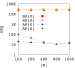
(a) Objects computed

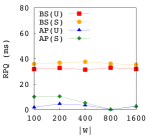
(b) Runtime

Figure 5: Effect of varying $|W|$ on Aus dataset

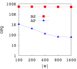
(a) Runtime

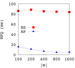
(b) Objects computed

Figure 6: Effect of varying $|W|$ on Foursq dataset

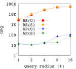
(a) Objects computed

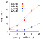
(b) Runtime

Figure 7: Effect of varying query radius on Aus dataset

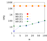
(a) Objects computed

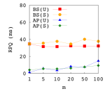
(b) Runtime

Figure 8: Effect of varying $m$ on Aus dataset

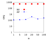
(a) Objects computed

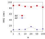
(b) Runtime

Figure 9: Effect of varying $m$ on Foursq dataset

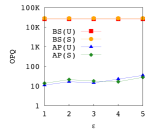
(a) Objects computed

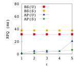
(b) Runtime

Figure 10: Effect of varying $\epsilon$ on Aus dataset

Figure 11: Effect of varying $B$ on Aus dataset

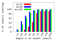
Figure 12: % of result overlap for varying $m$ in Aus dataset

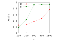
Figure 13: Index size vs. approximation ratio for varying $\epsilon$

Varying $|W|$

Figure 5 and Figure 6 show the impact of varying the number of queries in the sliding window, $|W|$, for Aus and Foursq, respectively. For Aus, the experiments were conducted using uniform and skewed query sets, while the Foursq query set is derived directly from user check-ins.

For both datasets, the number of popularity computations required by the approximate approach is about $3$ orders of magnitude less than the baseline. The reason is two-fold: (i) In the approximate approach, we compute the popularity of only the objects necessary to update the result. If the result objects of the previous window are found as valid, we do not need to compute the popularity of any additional object. In contrast, the baseline solution must update the popularity for all of the objects that satisfy the query constraint. (ii) Since the popularity function is an average aggregation (see Sec. 3), the popularity of an object usually does not change drastically as $|W|$ increases. Therefore, the result objects in a window are more likely to stay valid in subsequent windows for larger values of $|W|$, thereby requiring even fewer objects being checked. As shown in Figure 5b and Figure 6b, fewer popularity computation directly translates to lower running time.

In Aus, the performance in both uniform and skewed query sets improves $|W|$ increases, but drops slightly from $|W|=800$ to $|W|=1600$ for the approximate approach. The reason is that, if the results are not valid for a window, we need to look in the validation objects, which is a subset of the objects that satisfy the constraint of at least one query in the current window. So although the results update less often for larger $|W|$, an update in the results may require checking more objects for a larger $|W|$.

Varying query range

Figure 7 shows the performance when varying the radius of each query as a percentage of the dataspace. We vary the query radius only for Aus, as we use the radius that covers the check-in locations of a user as the query radius in the Foursq dataset. Here, the number of objects that fall into the query range grows as query radius increases. Therefore, the performance of the baseline declines rapidly when the query radius increases. In contrast, the approximate approach computes the popularity of only the objects that can be a result, which is a subset of the objects that fall within the query range. Thus, the approximate approach outperforms the baseline, and the benefit is more significant as the query radius increases.

Varying $m$

The experimental results when varying the number of result objects, $m$, are shown in Figure 8 and Figure 9 for Aus and Foursq, respectively. Here, the performance of the baseline does not vary much, as the baseline computes the popularity for all of the objects that fall within the query range regardless of the value of $m$. The approximate approach outperforms the baseline, because the approximate approach considers only the objects that can potentially be in the top-$m$ results. As more objects qualify to be a result, the performance of the approximate approach decreases with the increase of $m$.

Varying $\epsilon$

Figure 10 shows the performance of the approaches when varying the approximation parameter $\epsilon$ for Aus dataset. The approximate approach consistently outperforms the baseline for all choices of $\epsilon$. As the rank of an object is more accurately approximated for a smaller value of $\epsilon$, it leads to checking fewer number of objects and a lower runtime. As a result, the performance of the approximate approach gradually decreases with the increase of $\epsilon$.

Varying $B$

We vary the block size of the rank lists as the parameter $B$, and measure the performance. We find that the number of objects to check does not vary with $B$, because, if the result of a window needs to be updated, the same set of validation objects are retrieved regardless of the rank list block size Therefore, we only show the runtime for varying $B$ in Figure 11. For each $B$, the total runtime is shown as a breakdown of the computation time for (i) block-level safe rank, (ii) object-level safe rank, and (iii) validation object computation for both uniform and skewed query sets. From Figure 11 we can conclude that: (1) as the total number of blocks decreases for higher $B$, the time required to compute the block-level safe rank also decreases; and (2) the validation object lookups dominate the computational costs of the approximate solution.

6.3 Effectiveness Evaluation

Varying $m$

As shown in Figure 4a, the query locations originally follow a skewed distribution, and most of the query locations are clustered in a small area (which is the central business district of that city), while the rest of the queries are scattered regionally for Aus dataset. In the uniform query set, the queries are repeated uniformly, thus the upsized query set also follows the same (skewed) distribution of the original query set. For this reason, we evaluated our effectiveness as a percentage of result overlap when using the uniformly upsized query set to capture a more realistic scenario.

The percentage of result overlap between the top-$m$ approximate results and the top-$k$ exact results for Aus dataset are shown in Figure 12, where $k$ ranges from $10$ to $200$ and we set three choices of $m$ ($10$, $50$, $100$). We find that as $k$ increases, the overlap percentage also increases. For $m=50$ and $100$, the overlap percentage quickly reaches $90\%$ when $k=50$. Note that, if multiple objects have the same popularity value, we treat their rank position in the result as equivalent.

More experiment results on the percentage of result overlap for the Foursq dataset and the approximation ratio for both datasets for the varying $m$ can be found in Appendix B.

Varying query range

Please refer to Appendix B for the approximation ratio w.r.t varying query ranges.

Varying $\epsilon$, space vs. effectiveness tradeoff

Figure 13 shows the tradeoff between the space requirement and the effectiveness in terms of approximation ratio for varying $\epsilon$. Here, the x-axis represents the index size in GB for both datasets, where $\epsilon$ is varied from $1$ to $5$ at an interval of $1$. Since the approximate popularity of an object becomes closer to the exact popularity as $\epsilon$ decreases, the approximation ratio also improves for smaller $\epsilon$.

7 Conclusion

In this paper, we presented the problem of top-$m$ rank aggregation of spatial objects for streaming queries. We showed how to bound the rank of an object for any unseen query, and then proposed an exact solution for the problem. We then proposed an approximate solution with a guaranteed error bound, in which used safe ranking to determine whether the current result is still valid or not when new queries arrive, and validation objects to limit the number of objects to update in the top-$m$ results. We conducted a series of experiments on two real datasets, and show that the approximate approach is about $3$ orders of magnitude efficient than the exact solution on the collections, and the results returned by the approximate approach have more than a $90\%$ overlap with the exact solution for $m$ higher than $50$. Our work combines three important problem domains (rank aggregation, continuous queries and spatial databases) into a single context. In future work, we intend to continue exploring other spatial query constraints and rank aggregation functions using our framework in order to better understand how the interplay between these three important domains can be leveraged to solve other cross-disciplinary problems.

Appendix A Proof of approximation error bound

Proof.

Here, ${\bm{\hat{r}}}(o,q)$ is the average value of the ${\bm{r^{\,\downarrow}}}(o,c)$ and ${\bm{r^{\,\uparrow}}}(o,c)=(1+\epsilon)\times{\bm{r^{\,\downarrow}}}(o,c)$, where $c$ is the cell that contains $q$. Therefore, the difference between ${\bm{r}}(o,q)$ and ${\bm{\hat{r}}}(o,q)$ is maximum when ${\bm{r}}(o,q)={\bm{r^{\,\downarrow}}}(o,c)$ or ${\bm{r}}(o,q)={\bm{r^{\,\uparrow}}}(o,c)$.

From Equation 3, the difference between the exact and the approximate popularity computation of an object $o$ is derived from substituting the ${\bm{r}}(o,q)$ by ${\bm{\hat{r}}}(o,q)$ for each query $q$ in $W$. If $o$ does not satisfy ${\mbox{\em Con}}(q)$, the contribution to the popularity for $q$ is $0$ for both cases. Therefore, the difference between $\rho(o,W)$ and ${\bm{\hat{\rho}}}(o,W)$ is maximum when either (i) ${\bm{r}}(o,q_{i})={\bm{r^{\,\downarrow}}}(o,c_{i})$, or (ii) ${\bm{r}}(o,q_{i})={\bm{r^{\,\uparrow}}}(o,c_{i})$ for each $q_{i}$ in $W$. We denote $\lambda_{i}={\sum_{i=1}^{|W|}}{\bm{r^{\,\downarrow}}}(o,c_{i})$ for ease of presentation.

(i) If ${\bm{r}}(o,q_{i})={\bm{r^{\,\downarrow}}}(o,c_{i})$ for each $q_{i}$ in $W$, then

$$(1)\hphantom{1}\rho(o,W) =\frac{{\sum_{i=1}^{|W|}}N-{\bm{r^{\,\downarrow}}}(o,c_{i})+1}{|W|},\mbox{ and }$$

$$(2)\hphantom{1}{\bm{\hat{\rho}}}(o,W) =\frac{{\sum_{i=1}^{|W|}}N-(1+\epsilon/2)\times{\bm{r^{\,\downarrow}}}(o,c_{i})+1}{|W|}\mbox{ (from Eqn.~{}\ref{eqn:ar}).}$$

$$\rho(o,W)-{\bm{\hat{\rho}}}(o,W) =\frac{{\sum_{i=1}^{|W|}}-{\bm{r^{\,\downarrow}}}(o,c_{i})+(1+\epsilon/2){\bm{r^{\,\downarrow}}}(o,c_{i})}{\displaystyle|W|}$$

$$=\epsilon/2\times\frac{\displaystyle\lambda_{i}}{\displaystyle|W|}$$

$$\frac{\displaystyle\rho(o,W)}{\displaystyle\rho(o,W)-{\bm{\hat{\rho}}}(o,W)} =\frac{{\sum_{i=1}^{|W|}}N-{\bm{r^{\,\downarrow}}}(o,c_{i})+1}{\displaystyle\epsilon/2\times\lambda_{i}}$$

$$=\frac{\displaystyle W\times N+W-\lambda_{i}}{\displaystyle\epsilon/2\times\lambda_{i}}$$

Here, ${\bm{r^{\,\downarrow}}}(o,c)$ is the lower bound rank estimation, and the rank of an object is between $[1,N]$, hence, $W\leq\lambda_{i}\leq W\times N$. Therefore, the value of the nominator $W\times N+W-\lambda_{i}$ is also between $[W,W\times N]$. So by setting the lowest value of $\lambda_{i}$ in the equation, we get the following inequality,

$$\frac{\displaystyle\rho(o,W)}{\displaystyle\rho(o,W)-{\bm{\hat{\rho}}}(o,W)} \leq\frac{\displaystyle W\times N+W-W}{\displaystyle\epsilon/2\times W}$$

$$\leq\frac{\displaystyle N}{\displaystyle\epsilon/2}$$

$$\leq\frac{\displaystyle 2N}{\displaystyle\epsilon}$$

$$\Rightarrow\frac{\displaystyle\rho(o,W)-{\bm{\hat{\rho}}}(o,W)}{\displaystyle\rho(o,W)} \geq\frac{\displaystyle\epsilon}{\displaystyle 2N},\mbox{ (by taking the inverse)}$$

$$\Rightarrow 1-\frac{\displaystyle{\bm{\hat{\rho}}}(o,W)}{\displaystyle\rho(o,W)} \geq\frac{\displaystyle\epsilon}{\displaystyle 2N}$$

$$\Rightarrow\frac{\displaystyle{\bm{\hat{\rho}}}(o,W)}{\displaystyle\rho(o,W)} \leq 1-\frac{\displaystyle\epsilon}{\displaystyle 2N}$$

(ii) If ${\bm{r}}(o,q_{i})={\bm{r^{\,\uparrow}}}(o,c_{i})$ for each $q_{i}$ in $W$, then

$$(1)\hphantom{1}\rho(o,W) =\frac{{\sum_{i=1}^{|W|}}N-(1+\epsilon)\times{\bm{r^{\,\downarrow}}}(o,c_{i})+1}{|W|}\mbox{, and }$$

$$(2)\hphantom{1}{\bm{\hat{\rho}}}(o,W) =\frac{{\sum_{i=1}^{|W|}}N-(1+\epsilon/2)\times{\bm{r^{\,\downarrow}}}(o,c_{i})+1}{|W|}\mbox{ (from Eqn.~{}\ref{eqn:ar}). }$$

$${\bm{\hat{\rho}}}(o,W)-\rho(o,W) =\frac{{\sum_{i=1}^{|W|}}-(1+\epsilon/2)\times{\bm{r^{\,\downarrow}}}(o,c_{i})+(1+\epsilon)\times{\bm{r^{\,\downarrow}}}(o,c_{i})}{\displaystyle|W|}$$

$$=\epsilon/2\times\frac{\displaystyle\lambda_{i}}{\displaystyle|W|}$$

$$\frac{\displaystyle{\bm{\hat{\rho}}}(o,W)}{\displaystyle{\bm{\hat{\rho}}}(o,W)-\rho(o,W)} =\frac{{\sum_{i=1}^{|W|}}N-(1+\epsilon/2)\times{\bm{r^{\,\downarrow}}}(o,c_{i})+1}{\displaystyle\epsilon/2\times\lambda_{i}}$$

$$=\frac{\displaystyle W\times N+W-(1+\epsilon/2)\times\lambda_{i}}{\displaystyle\epsilon/2\times\lambda_{i}}$$

Setting the lowest value of $\lambda_{i}=W$ in the equation produces the following inequality,

$$\frac{\displaystyle{\bm{\hat{\rho}}}(o,W)}{\displaystyle{\bm{\hat{\rho}}}(o,W)-\rho(o,W)} \leq\frac{\displaystyle W\times N+W-(1+\epsilon/2)\times W}{\displaystyle\epsilon/2\times W}$$

$$\leq\frac{\displaystyle N-\epsilon/2}{\displaystyle\epsilon/2}$$

$$\Rightarrow\frac{\displaystyle{\bm{\hat{\rho}}}(o,W)-\rho(o,W)}{\displaystyle{\bm{\hat{\rho}}}(o,W)} \geq\frac{\displaystyle\epsilon/2}{\displaystyle N-\epsilon/2},\mbox{ (by taking the inverse)}$$

Since the value $\epsilon$ is between $[0,N-1]$, the denominator $N-\epsilon/2$ can be a maximum of $N$.

$$1-\frac{\displaystyle\rho(o,W)}{\displaystyle{\bm{\hat{\rho}}}(o,W)} \geq\frac{\displaystyle\epsilon/2}{\displaystyle N-\epsilon/2}\geq\frac{\displaystyle\epsilon/2}{\displaystyle N}$$

$$\Rightarrow\frac{\displaystyle\rho(o,W)}{\displaystyle{\bm{\hat{\rho}}}(o,W)} \leq 1-\frac{\displaystyle\epsilon}{\displaystyle 2N}$$

∎

Appendix B Additional experiment results

In this section, we show additional experiment results on our effectiveness study. Recall the experiment setting, although the primary purpose of the real country-level Foursq is to test out the scalability of our approximate and exact solution on real data, we also report its effectiveness results for the completeness of experiments.

Varying $|W|$

Table 3 shows the average approximation ratio for both datasets. Although the average approximation ratio gradually improves for both uniform and skewed query sets as $|W|$ increases, the change does not follow any obvious pattern. The explanation for this random behaviour is that popularity is an average aggregation of $|W|$ ranks, so if both the exact and the approximate popularity do not change at the same rate with $|W|$, their ratios do not change in a fixed way.

Varying $m$

Figure 15 shows the percentage of overlap between the top-$m$ approximate results and the top-$k$ exact results for Foursq dataset. Although the overlap becomes close to 100% for higher $m$, the overlap is not as good as the Aus dataset for lower values of $m$. The reason is as follows. As shown in Figure 4 the objects in Foursq are clustered into cities, and the cities are scattered in different parts of the USA. On the other hand, the query locations are distributed all over the dataspace, as a user can check-in at different cities. Therefore, the popularity values of most of the objects in a city are very close to each other. Figure 14 shows a screenshot of the top-$10$ popularities computed in the baseline approach at three example instances. As we can see, the final rank of two objects can be very far away for a slight difference in their popularity values; for example, in the first example instance, the difference between every adjacent objects’ popularity score is only 0.25 in average while the absolute values are at the scale of 50K.

Table 3: Approximation ratio for varying $|W|$

		100	200	400	800	1600
Aus	$U$	2.12	1.60	1.57	1.67	1.55
	$S$	3.19	1.55	2.14	1.30	1.34
Foursq		2.76	6.87	3.49	3.15	2.33

Table 4: Approximation ratio for varying $m$

		1	5	10	20	50	100
Aus	$U$	3.00	4.79	1.57	1.56	1.49	1.49
	$S$	5.61	2.03	2.14	1.60	1.17	1.16
Foursq		1.57	2.62	2.68	3.31	3.37	2.47

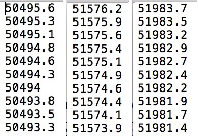
Figure 14: Popularity values of top-$10$ objects in Foursq dataset

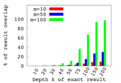
Figure 15: % of result overlap for varying $m$ in Foursq dataset

Table 4 shows the approximation ratio for varying $m$ for Aus dataset. As shown in the table, the approximation ratio keeps improving with the increase of $m$, probably because most objects in the top-$m$ ranked list have very similar scores in both their approximate popularity and approximate popularity when $m<100$. the top-$m$ ranked list are very close to each have very similar exact and approximate popularity scores.

Approximation ratio for varying query range

Table 5: Approximation ratio for varying query radius

		1	2	4	8	16
Aus	$U$	2.55	1.55	1.57	1.61	1.63
	$S$	3.32	2.88	2.14	2.39	3.55

The approximation ratio of the results w.r.t. varying query ranges are shown in Table 5. We find that the approximation ratio does not indicate any significant pattern for this parameter, because the approximation calculation does not depend on the query radius or the number of5objects falling within that range.

References

- Ailon et al. [2008] N. Ailon, M. Charikar, and A. Newman. Aggregating inconsistent information: ranking and clustering. JACM, 55(5):23, 2008.
- Bartholdi et al. [1989] J. J. Bartholdi, C. A. Tovey, and M. A. Trick. The computational difficulty of manipulating an election. Social Choice and Welfare, 6(3):227–241, 1989.
- Bohm et al. [2007] C. Bohm, B. C. Ooi, C. Plant, and Y. Yan. Efficiently processing continuous k-nn queries on data streams. In ICDE, pages 156–165, 2007.
- Cheema et al. [2012] M. Cheema, W. Zhang, X. Lin, Y. Zhang, and X. Li. Continuous reverse k nearest neighbors queries in euclidean space and in spatial networks. The VLDB Journal, 21(1):69–95, 2012.
- Cheema et al. [2010] M. A. Cheema, L. Brankovic, X. Lin, W. Zhang, and W. Wang. Multi-guarded safe zone: An effective technique to monitor moving circular range queries. In ICDE, pages 189–200, 2010.
- Chen-Yi et al. [2013] L. Chen-Yi, K. Jia-Ling, and A. P. Chen. Determining k-most demanding products with maximum expected number of total customers. TKDE, 25(8):1732–1747, 2013.
- Cormode and Hadjieleftheriou [2008] G. Cormode and M. Hadjieleftheriou. Finding frequent items in data streams. Proc. VLDB Endow., 1(2):1530–1541, 2008.
- Dwork et al. [2001] C. Dwork, R. Kumar, M. Naor, and D. Sivakumar. Rank aggregation methods for the web. In WWW, pages 613–622, 2001.
- Fagin et al. [2001] R. Fagin, A. Lotem, and M. Naor. Optimal aggregation algorithms for middleware. In PODS, pages 102–113, 2001.
- Fagin et al. [2003] R. Fagin, R. Kumar, and D. Sivakumar. Efficient similarity search and classification via rank aggregation. In SIGMOD, pages 301–312, 2003.
- Gkorgkas et al. [2013] O. Gkorgkas, A. Vlachou, C. Doulkeridis, and K. Nørvåg. Discovering influential data objects over time. In SSTD, pages 110–127, 2013.
- Guntzer et al. [2001] J. Guntzer, W. T. Balke, and W. Kiessling. Towards efficient multi-feature queries in heterogeneous environments. In ITCC, pages 622–628, 2001.
- Hasan et al. [2009] M. Hasan, M. A. Cheema, X. Lin, and Y. Zhang. Efficient construction of safe regions for moving knn queries over dynamic datasets. In SSTD, pages 373–379, 2009.
- Koh et al. [2014] J.-L. Koh, C.-Y. Lin, and A. P. Chen. Finding k most favorite products based on reverse top-t queries. PVLDB, 23(4):541–564, 2014.
- Korn et al. [2002] F. Korn, S. Muthukrishnan, and D. Srivastava. Reverse nearest neighbor aggregates over data streams. In VLDB Endowment, pages 814–825, 2002.
- Langville and Meyer [2012] A. Langville and C. Meyer. Who’s #1?: The Science of Rating and Ranking. Princeton University Press, 2012. ISBN 9781400841677.
- Lee and Ting [2006] L. K. Lee and H. F. Ting. A simpler and more efficient deterministic scheme for finding frequent items over sliding windows. In PODS, pages 290–297, 2006.
- Li et al. [2014a] C. Li, Y. Gu, J. Qi, G. Yu, R. Zhang, and W. Yi. Processing moving knn queries using influential neighbor sets. Proc. VLDB Endow., 8(2):113–124, 2014a.
- Li et al. [2014b] C.-L. Li, E. T. Wang, G.-J. Huang, and A. L. P. Chen. Top-n query processing in spatial databases considering bi-chromatic reverse k-nearest neighbors. Information Systems, 42:123–138, 2014b.
- Lin et al. [2013] H. Lin, F. Chen, Y. Gao, and D. Lu. OptRegion: Finding optimal region for bichromatic reverse nearest neighbors. In DASFAA, pages 146–160, 2013.
- Liu et al. [2011] H. Liu, Y. Lin, and J. Han. Methods for mining frequent items in data streams: an overview. Knowledge and Information Systems, 26(1):1–30, 2011.
- Mamoulis et al. [2006] N. Mamoulis, K. H. Cheng, M. L. Yiu, and D. W. Cheung. Efficient aggregation of ranked inputs. In ICDE, page 72, 2006.
- Mamoulis et al. [2007] N. Mamoulis, M. L. Yiu, K. H. Cheng, and D. W. Cheung. Efficient top-k aggregation of ranked inputs. ACM Trans. Database Syst., 32(3):19, 2007.
- Mouratidis and Papadias [2007] K. Mouratidis and D. Papadias. Continuous nearest neighbor queries over sliding windows. TKDE, 19(6):789–803, 2007.
- Mouratidis et al. [2005] K. Mouratidis, D. Papadias, and M. Hadjieleftheriou. Conceptual partitioning: an efficient method for continuous nearest neighbor monitoring. In SIGMOD, pages 634–645, 2005.
- Mouratidis et al. [2006] K. Mouratidis, S. Bakiras, and D. Papadias. Continuous monitoring of top-k queries over sliding windows. In SIGMOD, pages 635–646, 2006.
- Nutanong et al. [2010] S. Nutanong, R. Zhang, E. Tanin, and L. Kulik. Analysis and evaluation of v*-knn: an efficient algorithm for moving knn queries. The VLDB Journal, 19(3):307–332, 2010.
- Papapetrou et al. [2012] O. Papapetrou, M. Garofalakis, and A. Deligiannakis. Sketch-based querying of distributed sliding-window data streams. Proc. VLDB Endow., 5(10):992–1003, 2012.
- Pripužić et al. [2014] K. Pripužić, I. P. Žarko, and K. Aberer. Top-k/w publish/subscribe: A publish/subscribe model for continuous top-k processing over data streams. Information Systems, 39:256 – 276, 2014.
- Shekhar et al. [2016] S. Shekhar, S. K. Feiner, and W. G. Aref. Spatial computing. Comm. of the ACM, 59(1):72–81, 2016.
- Tao et al. [2007] Y. Tao, V. Hristidis, D. Papadias, and Y. Papakonstantinou. Branch-and-bound processing of ranked queries. Inf. Syst., 32(3):424–445, 2007.
- Vlachou et al. [2010] A. Vlachou, C. Doulkeridis, K. Nørvåg, and Y. Kotidis. Identifying the most influential data objects with reverse top-k queries. PVLDB, 3(1-2):364–372, 2010.
- Wong et al. [2009] R. C.-W. Wong, M. T. Özsu, P. S. Yu, A. W.-C. Fu, and L. Liu. Efficient method for maximizing bichromatic reverse nearest neighbor. PVLDB, 2(1):1126–1137, 2009.
- Xia et al. [2005] T. Xia, D. Zhang, E. Kanoulas, and Y. Du. On computing top-t most influential spatial sites. In VLDB Endowment, pages 946–957, 2005.
- Yan et al. [2011] D. Yan, R. C.-W. Wong, and W. Ng. Efficient methods for finding influential locations with adaptive grids. In CIKM, pages 1475–1484, 2011.
- Zhan et al. [2012] L. Zhan, Y. Zhang, W. Zhang, and X. Lin. Finding top k most influential spatial facilities over uncertain objects. In CIKM, pages 922–931, 2012.
- Zhou et al. [2011] Z. Zhou, W. Wu, X. Li, M. L. Lee, and W. Hsu. MaxFirst for MaxBRkNN. In ICDE, pages 828–839, 2011.