Minimax Filter: Learning to Preserve Privacy
from Inference Attacks

Abstract

Preserving privacy of continuous and/or high-dimensional data such as images, videos and audios, can be challenging with syntactic anonymization methods which are designed for discrete attributes. Differentially privacy, which uses a more rigorous definition of privacy loss, has shown more success in sanitizing continuous data. However, both syntactic and differential privacy are susceptible to inference attacks, i.e., an adversary can accurately infer sensitive attributes from sanitized data. The paper proposes a novel filter-based mechanism which preserves privacy of continuous and high-dimensional attributes against inference attacks. Finding the optimal utility-privacy tradeoff is formulated as a min-diff-max optimization problem. The paper provides an ERM-like analysis of the generalization error and also a practical algorithm to perform minimax optimization. In addition, the paper proposes a noisy minimax filter which combines minimax filter and differentially-private mechanism. Advantages of the method over purely noisy mechanisms is explained and demonstrated with examples. Experiments with several real-world tasks including facial expression classification, speech emotion classification, and activity classification from motion, show that the minimax filter can simultaneously achieve similar or higher target task accuracy and lower inference accuracy, often significantly lower than previous methods.

Keywords: inference attack, empirical risk minimization, minimax optimization, differential privacy, k-anonymity

1 Introduction

Privacy is an important issue when data collected from or related to individuals are analyzed and released to a third party. In response to growing privacy concerns, various methods for privacy-preserving data publishing have been proposed (see Fung et al. 2010 for a review.) Syntactic anonymization methods, such as $k$-anonymity (Sweeney, 2002) and $l$-diversity (Machanavajjhala et al., 2007) focus on anonymization of quasi-identifiers and protection of sensitive attributes in static databases. However, it is known that syntactic anonymization is susceptible to several types of attacks such as the DeFinetti attack (Kifer, 2009). An adversary may be able to accurately infer sensitive attributes of individuals from insensitive, sanitized attributes. High-dimensional data also poses a challenge for syntactic anonymization methods. For example, $k$-anonymity is known to be ineffective for high-dimensional sparse databases (Narayanan and Shmatikov, 2008). In addition, syntactic anonymization methods are designed with discrete attributes in mind. However, continuous attributes such as videos, images, or audios cannot be discretized by binning or clustering without loss of information. Besides, conventional categorization of attributes as identifiers, quasi-identifiers, or sensitive information becomes ambiguous with multimedia-type data. For example, an image can be an identifier if it contains the face of the data owner. However, even if the face is blurred, other attributes considered sensitive by the owner such as gender or race can still be recognizable. Furthermore, identifying or sensitive information can be revealed through correlation with other information such as the background or other people in the scene.

Differential privacy (Dwork and Nissim, 2004; Dwork et al., 2006; Dwork, 2006) was proposed to address many weaknesses of syntactic methods (see the discussion by Clifton and Tassa 2013.) Differential privacy has a more formal privacy guarantee than that of syntactic methods, and is applicable to many problems beyond database release (Dwork et al., 2014). In particular, differential privacy can be defined for continuous and/or high-dimensional attributes as well as for functions (Hall et al., 2013). However, similarly to syntactic anonymization, differential privacy is not immune to inference attacks (Cormode, 2011), as differentially privacy only prevents an adversary from gaining additional knowledge by inclusion/exclusion of a subject (Dwork et al., 2014), and not from gaining knowledge from released data itself. Therefore, an adversary may still guess sensitive attributes of subjects from differentially-private attributes with confidence.

To preserve privacy of continuous high dimensional data from inference attacks, this paper proposes an approach which differs significantly from previous syntactic or differentially-private approaches. Consider a scenario where a social media user wants to obfuscate all faces in her picture with minimal distortion before posting the picture online. The obfuscation mechanism proposed in the paper is a type of filtering of the original features by a non-invertible transformation. How to choose an optimal filter is explained in the following general description. Once the filtered data (e.g., obfuscated pictures) are released, an adversary will try to infer sensitive or identifying attributes from the data in particular using machine learning predictors. Therefore the data owner needs a filter that can minimize the maximum accuracy that any adversary may achieve in predicting the sensitive or identifying attributes. This is an instance of minimax games between the data owner and the adversary. The privacy of filtered data is measured by the expected risk of adversarial algorithms on specific inference tasks such as identification. However, if privacy is the only goal, near-perfect privacy is achievable with a simple mechanism that sends no or garbage data, which has no utility for any party. To avoid those trivial solutions, (dis)utility of filtered data needs to be considered as the second goal. Disutility can be measured by the amount of distortion of the original data after filtering. Alternatively, if there are particular tasks of interest to be performed on the data by non-adversarial analysts, then again the expected risk of the target tasks can be used as disutility. The two goals—achieving privacy and utility—are often mutually conflicting, and finding an optimal tradeoff between the two is a central question in privacy research (see Related work.) This paper proposes to minimize the difference of two risks by the minimax optimization of (7). The solution to the optimization problem will be referred to as minimax filter. In the literature, several methods have been used to solve continuous minimax optimization problems, including the method by Kiwiel (1987) used in Hamm (2015). The paper uses a simpler optimization method based on the classic theorem of Danskin (1967).

A notable assumption this paper makes is that the training data for computing an optimal filter are independent of the test data. For example, there are publicly available data sets that can be used to compute minimax filters such as those from the UCI data repository. As the training data set is already public information, the paper considers only the privacy of the subjects who use the filter at test time. A similar assumption was made in Hamm et al. (2016) for knowledge transfer purposes. After the filter is learned from training data, a new test subject can use the filter to obfuscate her data by herself without requiring a third party to collect and process her raw data. Note that this setting is analogous to the setting of local differential privacy (Duchi et al., 2013) where the entity that collects data is not trusted. Since the training procedure can only access empirical risks, the performance of the filter on test data is given in the form of expectation/probability. The paper presents an analysis of generalization error for empirical minimax optimizers in analogy with the analysis of empirical risk minimizers (ERM).

The goal of minimax filter is to prevent inference attacks, and its privacy guarantee is quite different from those of other privacy mechanisms. It is task-dependent and is given in probability or expectation rather than given absolutely, which may be considered weaker than other privacy criteria such as differential privacy. Furthermore, the sanitized data whose sensitive information is filtered out may become unsafe in the future if people’s perception of which attribute is sensitive changes over time. Since the goal of minimax filter and the goal of differential privacy are very different, it is natural to ask if the two methods can be combined to take advantages of both methods. Consequently, this paper presents an extension of minimax filter called noisy minimax filter, which combines the filter with additive noise mechanism to satisfy the differential privacy criterion. Two methods of combination—preprocessing and postprocessing—are proposed (see Fig. 2.) In the preprocessing approach, minimax filter is applied before perturbation to reduce the sensitivity of transformed data, so that the same level of differential privacy is achieved with less noise. Similar ideas have been utilized before, where data are transformed by Discrete Fourier Transform (Rastogi and Nath, 2010) and by Wavelet Transform (Xiao et al., 2011) before noise is added. In the postprocessing approach, minimax filter is applied after perturbation, and its performance is compared with the preprocessing approach.

Minimax filter and its extensions are evaluated with several real-world tasks including facial expression classification, speech emotion classification, and activity classification from motion. Experiments show that publicly available continuous and high-dimensional data sets are surprisingly susceptible to subject identification attacks, and that minimax filters can reduce the privacy risks to near chance levels without sacrificing utility much. Experiments with noisy minimax filter also yield intuitive results. Differential privacy and resilience to inference attack are indeed different goals, such that using differentially private mechanism alone to achieve the latter requires a large amount of noise that destroys utility of data. In contrast, minimax filters can suppress inference attack with little loss of utility with or without perturbation. Therefore, adding a small amount of noise to the minimax filter can provide a formal differential privacy to a degree and also high on-average task-dependent utility and privacy against inference attacks.

To summarize, the paper has the following contributions.

• The paper proposes a novel filtering approach which preserves privacy of continuous and high-dimensional attributes against inference attacks. This mechanism is different from previous mechanisms in many ways; in particular, it is a learning-based approach and is task-dependent.

• The paper measures utility and privacy by expected risks, and formulates the utility-privacy tradeoff as a min-diff-max optimization problem. The paper provides an ERM-like analysis of the generalization performance of empirical optimizers.

• The paper presents a practical algorithm which can find minimax filters for a broad family of filters and losses/classifiers. The proposed optimization algorithm and supporting classes can be found on the open-source repository.

• The paper proposes preprocessing and postprocessing approaches to combine minimax filter with noisy mechanisms. The resulting combination can achieve resilience to inference attacks and differential privacy at the same time.

• The paper evaluates proposed algorithms on real-world tasks and compares them with representative algorithms from the literature.

The rest of the paper is organized as follows. Sec. 2 presents related work in the literature. Sec. 3 presents minimax filters and analyzes its generalization performance on test data. Sec. 4 explains the difficulty of solving general minimax problems, and present a simple alternating optimization algorithm. Sec. 5 presents noisy minimax filters and two types of perturbation by additive noise. Sec. 6 evaluates minimax filters with three data sets compared to non-minimax approaches and also evaluates noisy minimax filters under various conditions. Sec. 7 concludes the paper with discussions.

2 Related work

Optimal utility-privacy tradeoff is one of the main goals in privacy research. Utility-privacy tradeoff has particularly been well-studied under differential privacy assumptions (Dwork and Nissim, 2004; Dwork et al., 2006; Dwork, 2006), in the context of the statistical estimation (Smith, 2011; Alvim et al., 2012; Duchi et al., 2013) and learnability (Kasiviswanathan et al., 2011). Other measures of privacy and utility were also proposed. Information-theoretic quantities were proposed by Sankar et al. (2010); Rebollo-Monedero et al. (2010); du Pin Calmon and Fawaz (2012) who analyzed privacy in terms of the rate-distortion theory in communication. One problem with using mutual information or related quantity is that it is difficult to estimate mutual information of high-dimensional and continuous variables in practice without assuming a simple distribution. In contrast, this paper proposes to use classification or regression risks to measure privacy and utility, which is directly computable from data without making assumptions on the distribution. Regarding the use of risks in this paper, classification error-based quantities have been suggested in the literature (Iyengar, 2002; Brickell and Shmatikov, 2008; Li and Li, 2009). However, privacy in those works is measured either by syntactic anonymity or probabilistic divergence which are mainly suitable for discrete attributes. In this paper, privacy and utility are both defined using risks and are therefore directly comparable when defining the tradeoff of the two. Furthermore, the proposed method explicitly preserves privacy against inference attacks, which both syntactic and differentially-private methods are known to be susceptible to (Cormode, 2011).

Most of the aforementioned works focused on the analyses of utility-privacy tradeoff using different measures and assumptions. Few studied efficient algorithms to actively find optimal tradeoff which this paper aims to do. For discrete variables, Krause and Horvitz (2008) showed the NP-hardness of optimal utility-privacy tradeoff in discrete attribute selection, and demonstrated near-optimality of greedy selection. In particular, they used a weighted difference of utility and privacy cost as the joint cost similar to this work. Ghosh et al. (2009) proposed geometric mechanism and linear programming to achieve near-optimal utility for unknown users. Note that the optimization problems with discrete distributions are quite different from the problems involving high-dimensional and/or continuous distributions.

Algorithms for preserving privacy of high-dimensional face images has been proposed previously. Newton et al. (2005) applied k-anonymity to images; Enev et al. (2012) proposed to learn a linear filter using Partial Least Squares to reduce the covariance between filtered data and private labels; Whitehill and Movellan (2012) also proposed a linear filter using the log-ratio of the Fisher’s Linear Discriminant Analysis metrics. Xu et al. (2017) presented a related method of preserving privacy of linear predictors using the Augmented Fractional Knapsack algorithm. This paper differs from these in several aspects: it is not limited to linear filters and is applicable to arbitrary differentiable nonlinear filters such as multilayer neural networks; it directly optimizes the utility-privacy risk instead of optimizing heuristic criteria such as covariance differences or LDA log-ratios.

The noisy minimax filter proposed in Sec. 5 bears a resemblance to the work of Rastogi and Nath (2010) and Xiao et al. (2011). Rastogi and Nath (2010) presented a differentially private method of answering queries on time-series data. They used Discrete Fourier Transform to reduce the data dimension and homomorphic encryption to perform distributed noise addition which outperformed the naive noise addition method. Xiao et al. (2011) presented a differentially private range-counting method where they used wavelets to transform the data before adding noise. Effectiveness of the method was analyzed and also demonstrated empirically. The noisy minimax filter presented in this paper, especially the preprocessing approach, is similar in concept to those works in that the combination of data transformation and perturbation is used to enhance utility. However, the transform in this paper (i.e., the minimax filter) is learned from data for specific tasks unlike the Fourier or the Wavelet transform which are data and task independent.

Lastly, the alternating optimization algorithm (Alg. 1) presented in this paper is related to the algorithm proposed by Goodfellow et al. (2014). The algorithm proposed in this paper solves a min-diff-max problem to find an optimal utility-privacy tradeoff, while Goodfellow et al. (2014) solve a minimax problem to learn generative models.

Parts of this paper have appeared in conference proceedings (Hamm, 2015, 2017). New materials in this paper include reformulations of concepts and terms, ERM-like analysis of generalization error, new closed-form examples for minimax optimization, and an alternating optimization algorithm to solve minimax problems.

3 Minimax Filter

In this section, minimax filter is introduced and discussed in detail, and its generalization error is analyzed.

3.1 Formulation

Minimax filter is a non-invertible transformation of raw features/attributes such that the transformed data have optimal utility-privacy tradeoff. Non-invertibility is assumed so that original features are not always recoverable from the filtered data. Let’s assume the filter is deterministic; randomize filters will be discussed in Sec. 5. Let $\mathcal{X}\subset\mathbb{R}^{D}$ be the space of features/attributes as real-valued vectors. Note that discrete attributes can also be represented by real vectors, e.g., by one-hot vector. Let the filter be a map

$$g(x;u)\in G:\mathcal{X}\times\mathcal{U}\to\mathbb{R}^{d}$$ (1)

which is continuous in $x$ and is continuously differentiable w.r.t. the parameter $u\in\mathcal{U}$. Given a filtered output $g(x)$, an adversary can make a prediction $h_{p}(g(x);v)$ of a private variable $y$ which can be an identifying or sensitive attribute. The prediction function $h_{p}(g(x);v)$ parameterized by $v\in\mathcal{V}$ is also assumed to be continuous in $v$ and continuously differentiable w.r.t. to the input $g(x)$. The paper proposes to use expected risk to measure the privacy of filtered output against adversarial inference:

$$f_{\mathrm{priv}}(u,v)\triangleq E[l_{p}(h_{p}(g(x;u);v),y)],$$ (2)

where $l_{p}(\cdot)$ is a continuously differentiable loss function. From the assumptions above, $f_{\mathrm{priv}}$ is continuously differentiable w.r.t. the filter parameter $u$.

Trivial solutions to maximize privacy already exist, which are the filters that output random or constant numbers independent of actual data. However, such filters have no utility whatsoever for any party. To avoid such trivial solutions, it is necessary to consider the secondary goal of maximizing utility.

Suppose the disutility of filtered data is measured by the distortion of the original data. If $g(x;u)$ is the filter/encoder $\mathcal{X}\to\mathbb{R}^{d}$, then one can construct the decoder $h(\cdot\;;w):\mathbb{R}^{d}\to\mathcal{X}$, such that following reconstruction error

$$f_{\mathrm{util}}(u,w)\triangleq E[\|h_{u}(g(x;u);w)-x\|^{2}],$$ (3)

is minimized (i.e., $\min_{w}f_{\mathrm{util}}(u,w)$.)

For another example of utility, let $z$ be a target variable that is of interest to the subjects and analysts such as medical diagnosis of users’ data. An analyst can make a prediction $h_{u}(g(x);w)$ parameterized by $w\in\mathcal{W}$, which is assumed to be continuous in $w$ and continuously differentiable w.r.t. the input $g(x)$. The (dis)utility of the filtered output for a non-adversarial analyst can also be measured by the expected risk

$$f_{\mathrm{util}}(u,w)\triangleq E[l_{u}(h_{u}(g(x;u);w),z)],$$ (4)

where $l_{u}(\cdot)$ is a continuously differentiable loss function, such that $f_{\mathrm{util}}$ is continuously differentiable w.r.t. the filter parameter $u$. To facilitate the analysis, the paper assumes that the constraint sets $\mathcal{W}$, $\mathcal{V}$, and $\mathcal{U}$ are compact and convex subsets of Euclidean spaces such as a ball with a large but finite radius. Along with the assumption that the filter $g$ and the risks $f_{\mathrm{priv}}$ and $f_{\mathrm{util}}$ are all continuous, min and max values are bounded and attainable. In addition, the solutions to min or max problems are assumed to be in the interior of $\mathcal{W}$, $\mathcal{V}$, and $\mathcal{U}$, enforced by adding appropriate regularization (e.g, $\lambda\|w\|^{2}$) to the optimization problems if necessary. For this reason, min or max problems that appear in the paper will be treated as unconstrained and the notations $u\in\mathcal{U}$, $v\in\mathcal{V}$, and $w\in\mathcal{W}$ will be omitted.

Having defined the privacy measure and the utility measure, the goal of a filter designer is to find a filter that achieves the following two objectives. The first objective is to maximize privacy

$$\max_{u}\min_{v}f_{\mathrm{priv}}(u,v)\;\;\;(\mathrm{or}\;\mathrm{equivalently,}\;\;\min_{u}\max_{v}-f_{\mathrm{priv}}(u,v))$$ (5)

where $\min_{v}f_{\mathrm{priv}}(u,v)$ represents the risk of the worst (i.e., most capable) adversary: the smaller the risk, the more accurately can she infer the sensitive variable $y$. As mentioned before, this problem alone has a trivial solution such as a constant filter that outputs zeros. The second objective is to minimize disutility

$$\min_{u}\min_{w}f_{\mathrm{util}}(u,w)\;\;\;(\mathrm{or}\;\mathrm{equivalently,}\;\;\min_{u}-\max_{w}-f_{\mathrm{util}}(u,w))$$ (6)

where $\min_{w}f_{\mathrm{util}}(u,w)$ represents the risk of the best analyst: the smaller the risk, the more accurately can the analyst reconstruct original data $x$ or predict the variable of interest $z$. To achieve the two opposing goals, we can solve the joint problem of minimizing the weighted sum

$$\min_{u}\;\left[\max_{v}-f_{\mathrm{priv}}(u,v)+\rho\;\min_{w}f_{\mathrm{util}}(u,w)\right],$$ (7)

or equivalently the weighted difference of max values

$$\min_{u}\;\left[\max_{v}-f_{\mathrm{priv}}(u,v)-\rho\max_{w}-f_{\mathrm{util}}(u,w)\right].$$ (8)

The constant $\rho>0$ determines the relative importance of utility versus privacy. For a small $\rho\ll 1$, the problem is close to a trivial privacy-only task, and for a large $\rho\gg 1$, the problem is close to a utility-only task. The solution to (7) or (8) will be referred to as minimax filter and is by definition an optimal filter for utility-privacy tradeoff in terms of expected risks given the family of filters $\{g(\cdot\;;u)|u\in\mathcal{U}\}$, the family of private losses/classifiers $\{l_{p}(h_{p}(\cdot\;;v))|v\in\mathcal{V}\}$ and the family of utility losses/classifiers $\{l_{u}(h_{u}(\cdot\;;w))|w\in\mathcal{W}\}$. Note that the choice of filter and loss/classifier families is very flexible, with the assumption of differentiability only. In practice, almost-everywhere differentiability suffices to use the algorithm in the paper. Fig. 1 shows an example filter/classifier from the class of multilayer neural networks. As an aside, the joint problem may be formulated as minimization of disutility with a hard constraint on privacy risk. When using interior-point methods, the procedure is similar to solving (8) iteratively with an increasing $\rho$, which is more demanding than minimizing the weighted sum only once as the paper proposes.

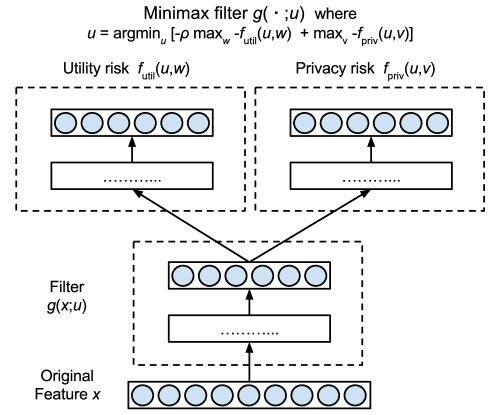
Figure 1: Minimax filter with a filter/classifiers from the class of multilayer neural networks.

3.2 Notes on private and utility tasks

The private variable $y$ can be any attribute which is considered sensitive or identifying. For example, let $y$ be any number or string unique to a person in the data set. Such identifiers are bijective with $\{1,...,S\}$, where $S$ is the total number of subjects, so assume $y\in\{1,...,S\}$. The private task for an adversary is then to predict the subject number $y$ from the filtered data $g(x)$, whose inaccuracy is measured by the expected risk of the identification task. That is, the less accurate the private classifier is, the more anonymous the filtered output is. The identity variable can also be group identifiers, e.g., $y$ is a demographic grouping based on age, sex, ethnicity, etc. Another example of private tasks is to single-out a particular subject among the rest, in which case $y$ is binary: $y=-1$ means ‘not the target subject’ and $y=1$ means ‘target subject’. To summarize, anonymity of filtered data in this paper means resilience to inference attacks on any variable $y$ that we choose. This unifying approach is convenient since we need not determine whether an attribute is an identifier, a quasi-identifier or a sensitive attribute as in syntactic anonymization. Any information hidden in the continuous high-dimensional features which are relevant to the private variable $y$—whatever it may be—will be maximally filtered out by construction. Similarly, the target variable $z$ of interest can be any variable that is not the same as the private variable $y$. In the pathological case where they are the same ($z=y$), the objective (8) becomes

$$\min_{u}\;\left[(1-\rho)\max_{v}-f(u,v)\right]$$ (9)

which is either a trivial privacy-only problem when $0\leq\rho<1$, or a utility-only problem when $\rho>1$. In general, $z$ and $y$ will be correlated to a certain degree, and the minimax filter will find the best compromise of utility and privacy risks.

Also, private and target tasks need not be classification tasks only. Regression tasks can also be used as a target task, as well as unsupervised tasks that do not require label $z$. Unsupervised tasks are useful when the target task is unknown or non-specific. For example, (3) measures the expected least-squares error between the original and the reconstructed features.

3.3 Multiple tasks

Extension of the idea in the previous section to multiple private and target tasks is straightforward. Suppose there are $N_{p}$ private tasks $f_{\mathrm{priv}}^{1}(u,v_{1}),...,f_{\mathrm{priv}}^{N_{p}}(u,v_{Np})$ associated with private random variables $y^{1},...,y^{Np}$. Note that $f_{\mathrm{priv}}^{i}(u,v_{i})=E[l_{p}^{i}(h^{i}(g(x;u);v_{i}),y^{i})]$. Similarly, suppose there are $N_{u}$ target tasks $f_{\mathrm{util}}^{1}(u,w_{1}),...,f_{\mathrm{util}}^{N_{u}}(u,w_{Nu})$ associated with target random variables $z_{1},...,z_{Nu}$. If $\kappa_{1},...,\kappa_{Np}$ are the coefficients representing relative importance of private tasks, and $\rho_{1},...,\rho_{Nu}$ are the coefficients for utility tasks, then the final objective is to solve the following problem

$$\min_{u}\;\left[\sum_{i=1}^{N_{p}}\kappa_{i}\max_{v_{i}}-f_{\mathrm{priv}}^{i}(u,v_{i})\;+\;\sum_{i=1}^{N_{u}}\rho_{i}\min_{w_{i}}f_{\mathrm{util}}^{i}(u,w_{i})\;\right].$$ (10)

Since this can be rewritten as

$$\min_{u}\;\left[\max_{v_{1},...,v_{N_{p}}}-\sum_{i=1}^{N_{p}}\kappa_{i}f_{\mathrm{priv}}^{i}(u,v_{i})\;+\;\min_{w_{1},...,w_{N_{u}}}\sum_{i=1}^{N_{u}}\rho_{i}f_{\mathrm{util}}^{i}(u,w_{i})\;\right],$$ (11)

this multiple task problem is nearly identical to the original single task problem (7), with the new utility and privacy tasks defined as

$$\hat{f}_{\mathrm{priv}}(u,v\mathrm{=}(v_{1},...,v_{Np})) \triangleq \sum_{i}\kappa_{i}f_{\mathrm{priv}}^{i}(u,v_{i}),\;\;\mathrm{and}$$ (12)

$$\hat{f}_{\mathrm{util}}(u,w\mathrm{=}(w_{1},...,w_{Nu})) \triangleq \sum_{i}\rho_{i}f_{\mathrm{util}}^{i}(u,w_{i}),$$ (13)

with $\rho=1$. Using this, it is straightforward to extend the analysis and algorithms developed for single tasks to those for multiple tasks.

3.4 Generalization performance of minimax filter

The proposed privacy mechanism is a learning-based approach. An optimal filter is one that solves the expected risk optimization (7). However, in reality, an optimal filter has to be estimated from finite training samples, and we need a guarantee on the performance of the learned filter on unseen test samples. This section derives generalization bounds for empirical minimax filter similar to the derivation of bounds for empirical risk minimizers (ERM).

The joint problem for expected risks was

$$\min_{u}\left[\max_{v}-f_{\mathrm{priv}}(u,v)+\rho\min_{w}f_{\mathrm{util}}(u,w)\right]\\ =\min_{u}\left[\max_{v}-E[l_{p}(u,v)]+\rho\min_{w}E[l_{u}(u,w)]\right].$$ (14)

A joint loss $l_{J}$ is introduced for convenience:

$$l_{J}(u,v,w)\triangleq-l_{p}(u,v)+\rho\;l_{u}(u,w).$$ (15)

Let $(u^{\ast},v^{\ast},w^{\ast})$ be a solution to the expected risk optimization problem:

$$E_{D}[l_{J}(u^{\ast},v^{\ast},w^{\ast})]=\min_{u}\left[\max_{v}E_{D}[-l_{p}(u,v)]+\rho\min_{w}E_{D}[l_{u}(u,w)]\right],$$ (16)

where $E_{D}[\cdot]$ is the expected value w.r.t. the unknown data distribution $P(x,y)$. Similarly, let $(\hat{u},\hat{v},\hat{w})$ be a solution to the empirical risk minimax problem:

$$E_{S}[l_{J}(\hat{u},\hat{v},\hat{w})]=\min_{u}\left[\max_{v}E_{S}[-l_{p}(u,v)]+\rho\min_{w}E_{S}[l_{u}(u,w)]\right],$$ (17)

where the empirical mean $E_{S}[\cdot]$ for $S=\{(x_{1},y_{1}),\cdots,(x_{N},y_{N})\}$ is

$$E_{S}[l(x,y)]\triangleq\frac{1}{N}\sum_{(x,y)\in S}l(x,y).$$ (18)

The goal in this analysis is to show that the expected and the empirical optimizers perform equally well in expectation/probability given enough training samples:

$$E_{D}[l_{J}(\hat{u},\hat{v},\hat{w})]\simeq E_{D}[l_{J}(u^{\ast},v^{\ast},w^{\ast})],\;\;\mathrm{as}\;\;N\to\infty.$$ (19)

The main result is the Theorem 4 which is proved in the remainder of this section. Let’s define optimal parameters $v(u)$ and $w(u)$ given $u$ as

$$v^{\ast}(u) \triangleq \arg\max_{v}E_{D}[-l_{p}(u,v)],\;\;\;\;\;\hat{v}(u)\;\;\triangleq\;\;\arg\max_{v}E_{S}[-l_{p}(u,v)],$$ (20)

$$w^{\ast}(u) \triangleq \arg\min_{w}E_{D}[l_{u}(u,w)],\;\;\;\;\;\;\;\hat{w}(u)\;\;\triangleq\;\;\arg\min_{w}E_{S}[l_{u}(u,w)].$$ (21)

One can then write

$$E_{D}[l_{J}(u^{\ast},v^{\ast},w^{\ast})] = \min_{u}\left[E_{D}[-l_{p}(u,v^{\ast}(u))]+\rho E_{D}[l_{u}(u,w^{\ast}(u))\right]]$$ (22)

$$= \min_{u}E_{D}[l_{J}(u,v^{\ast}(u),w^{\ast}(u))],$$ (23)

and similarly

$$E_{S}[l_{J}(\hat{u},\hat{v},\hat{w})]=\min_{u}\left[E_{S}[-l_{p}(u,\hat{v}(u))]+\rho E_{S}[l_{u}(u,\hat{w}(u))]\right]=\min_{u}E_{S}[l_{J}(u,\hat{v}(u),\hat{w}(u))].$$ (24)

From these definitions we have for all $u$,

$$E_{D}[l_{J}(u^{\ast},v^{\ast},w^{\ast})] \leq E_{D}[l_{J}(u,v^{\ast}(u),w^{\ast}(u))],$$ (25)

$$E_{S}[l_{J}(\hat{u},\hat{v},\hat{w})] \leq E_{S}[l_{J}(u,\hat{v}(u),\hat{w}(u))].$$ (26)

Also from definition, for all $(u,v,w)$,

$$E_{D}[l_{J}(u,v,w^{\ast}(u))] \leq E_{D}[l_{J}(u,v,w)]\;\leq\;E_{D}[l_{J}(u,v^{\ast}(u),w)],$$ (27)

$$E_{S}[l_{J}(u,v,\hat{w}(u))] \leq E_{S}[l_{J}(u,v,w)]\;\leq\;E_{S}[l_{J}(u,\hat{v}(u),w)].$$ (28)

These observations imply the following theorem.

Theorem 1

The risk difference of expected and empirical optimizers is at most twice the largest difference of expected and empirical risks of any set of parameters:

$$|E_{D}[l_{J}(\hat{u},\hat{v},\hat{w})]-E_{D}[l_{J}(u^{\ast},v^{\ast},w^{\ast})]|\leq 2\sup_{u,v,w}\left|E_{D}[l_{J}(u,v,w)]-E_{S}[l_{J}(u,v,w)]\right|.$$ (29)

Proof  The expected risk of empirical risk optimizers $(\hat{u},\hat{v},\hat{w})$ is upper-bounded by the risk of expected risk optimizers $(u^{\ast},v^{\ast},w^{\ast})$ as follows:

$$E_{D}[l_{J}(\hat{u},\hat{v},\hat{w})]-E_{D}[l_{J}(u^{\ast},v^{\ast},w^{\ast})]$$

$$= E_{D}[l_{J}(\hat{u},\hat{v},\hat{w})]-E_{S}[l_{J}(\hat{u},\hat{v},\hat{w})]-\left(E_{D}[l_{J}(u^{\ast},v^{\ast},w^{\ast})]-E_{S}[l_{J}(\hat{u},\hat{v},\hat{w})]\right)$$

$$\leq E_{D}[l_{J}(\hat{u},\hat{v},\hat{w})]-E_{S}[l_{J}(\hat{u},\hat{v},\hat{w})]-\left(E_{D}[l_{J}(u^{\ast},v^{\ast},w^{\ast})]-E_{S}[l_{J}(u^{\ast},\hat{v}(u^{\ast}),\hat{w}(u^{\ast}))]\right)\;\;(\mathrm{from}\;(\ref{eq:ineq2}))$$

$$\leq E_{D}[l_{J}(\hat{u},\hat{v},\hat{w})]-E_{S}[l_{J}(\hat{u},\hat{v},\hat{w})]-\left(E_{D}[l_{J}(u^{\ast},\hat{v}(u^{\ast}),w^{\ast})]-E_{S}[l_{J}(u^{\ast},\hat{v}(u^{\ast}),\hat{w}(u^{\ast}))]\right)\;\;(\mathrm{from}\;(\ref{eq:ineq3}))$$

$$\leq E_{D}[l_{J}(\hat{u},\hat{v},\hat{w})]-E_{S}[l_{J}(\hat{u},\hat{v},\hat{w})]-\left(E_{D}[l_{J}(u^{\ast},\hat{v}(u^{\ast}),w^{\ast})]-E_{S}[l_{J}(u^{\ast},\hat{v}(u^{\ast}),w^{\ast})]\right)\;\;(\mathrm{from}\;(\ref{eq:ineq4}))$$

$$\leq 2\sup_{u,v,w}\left|E_{D}[l_{J}(u,v,w)]-E_{S}[l_{J}(u,v,w)]\right|.$$

The difference can also be lower-bounded as follows:

$$E_{D}[l_{J}(u^{\ast},v^{\ast},w^{\ast})]-E_{D}[l_{J}(\hat{u},\hat{v},\hat{w})]$$

$$= E_{D}[l_{J}(u^{\ast},v^{\ast},w^{\ast})]-E_{S}[l_{J}(\hat{u},\hat{v},\hat{w})]-\left(E_{D}[l_{J}(\hat{u},\hat{v},\hat{w})]-E_{S}[l_{J}(\hat{u},\hat{v},\hat{w})]\right)$$

$$\leq E_{D}[l_{J}(\hat{u},v^{\ast}(\hat{u}),w^{\ast}(\hat{u}))]-E_{S}[l_{J}(\hat{u},\hat{v},\hat{w})]-\left(E_{D}[l_{J}(\hat{u},\hat{v},\hat{w})]-E_{S}[l_{J}(\hat{u},\hat{v},\hat{w})]\right)\;\;(\mathrm{from}\;(\ref{eq:ineq1}))$$

$$\leq E_{D}[l_{J}(\hat{u},v^{\ast}(\hat{u}),w^{\ast}(\hat{u}))]-E_{S}[l_{J}(\hat{u},v^{\ast}(\hat{u}),\hat{w})]-\left(E_{D}[l_{J}(\hat{u},\hat{v},\hat{w})]-E_{S}[l_{J}(\hat{u},\hat{v},\hat{w})]\right)\;\;(\mathrm{from}\;(\ref{eq:ineq4}))$$

$$\leq E_{D}[l_{J}(\hat{u},v^{\ast}(\hat{u}),\hat{w})]-E_{S}[l_{J}(\hat{u},v^{\ast}(\hat{u}),\hat{w})]-\left(E_{D}[l_{J}(\hat{u},\hat{v},\hat{w})]-E_{S}[l_{J}(\hat{u},\hat{v},\hat{w})]\right)\;\;(\mathrm{from}\;(\ref{eq:ineq3}))$$

$$\leq 2\sup_{u,v,w}\left|E_{D}[l_{J}(u,v,w)]-E_{S}[l_{J}(u,v,w)]\right|.$$

 
To bound the RHS of (29), one can use the Rademacher complexity theory (e.g., Lemma 26.2 of Shalev-Shwartz and Ben-David (2014).)

Lemma 2

Let $F$ be a class of real-valued functions, and let $S$ be a set of $N$ samples $S=\{(x_{1},y_{1}),...,(x_{N},y_{N})\}$. Then,

$$E_{S\sim D^{N}}\left[\sup_{f\in F}|E_{D}[f]-E_{S}[f]|\right]\leq 2E_{S\sim D^{N}}[\mathfrak{R}(F\circ S)],$$ (30)

where $\mathfrak{R}(F\circ S)$ is the empirical Rademacher complexity

$${\mathfrak{R}}(f\circ S)\triangleq\frac{1}{N}E_{\sigma\sim\{-1,+1\}^{N}}\left[\sup_{f\in F}\sum_{i=1}^{N}\sigma_{i}f(x_{i},y_{i})\right]$$ (31)

for the class of real-valued functions $\{(x,y)\mapsto f(x,y)\;:\;\forall f\in F\}$.

Consider the class of real-valued functions defined from the joint loss (15):

$$l_{J}\circ H_{J}\circ S \triangleq \{(x,y,z)\mapsto l_{J}(x,y,z;u,v,w)\;:\;u\in\mathcal{U},v\in\mathcal{V},w\in\mathcal{W}\}$$

$$= \{(x,y,z)\mapsto-l_{p}(h_{v}(g_{u}(x)),y)+\rho\;l_{u}(h_{w}(g_{u}(x)),z)\;:\;u\in\mathcal{U},v\in\mathcal{V},w\in\mathcal{W}\}.$$

Let ${\mathfrak{R}}(l_{J}\circ H_{J}\circ S)$ denote the empirical Rademacher complexity of the joint loss class. Furthermore, the Rademacher complexity of sum of functions can be upper-bounded by the sum of complexities:

Lemma 3

The empirical Rademacher complexity of the joint privacy-utility loss is upper-bounded as

$$\mathfrak{R}(l_{J}\circ H_{J}\circ S)\leq\mathfrak{R}(l_{p}\circ H_{p}\circ G\circ S)+\rho\;\mathfrak{R}(l_{u}\circ H_{u}\circ G\circ S),\;\;\;(\rho>0)$$ (33)

where

$$l_{p}\circ H_{p}\circ G\circ S \triangleq \{(x,y,z)\mapsto l_{p}(h_{p}(g_{u}(x)),y)\;:\;u\in\mathcal{U},v\in\mathcal{V}\},$$ (34)

$$l_{u}\circ H_{u}\circ G\circ S \triangleq \{(x,y,z)\mapsto l_{u}(h_{u}(g_{u}(x)),z)\;:\;u\in\mathcal{U},w\in\mathcal{W}\}.$$ (35)

Proof 

$$\mathfrak{R}(l_{J}\circ H_{J}\circ S) = \frac{1}{N}E_{\sigma}\left[\sup_{u,v,w}\left|\sum_{i=1}^{N}\sigma_{i}l_{J}(x_{i},y_{i},z_{i};u,v,w)\right|\right]$$ (36)

$$= \frac{1}{N}E_{\sigma}\left[\sup_{u,v,w}\left|\sum_{i=1}^{N}\sigma_{i}(-l_{p}(x_{i},y_{i};u,v)+\rho\;l_{u}(x_{i},z_{i};u,w))\right|\right]$$ (37)

$$\leq \frac{1}{N}E_{\sigma}\left[\sup_{u,v}\left|\sum_{i=1}^{N}\sigma_{i}l_{p}(x_{i},y_{i};u,v)\right|+\rho\;\sup_{u,w}\left|\sum_{i=1}^{N}\sigma_{i}l_{u}(x_{i},z_{i};u,w)\right|\right]$$ (38)

$$= \mathfrak{R}(l_{p}\circ H_{p}\circ G\circ S)+\rho\;\mathfrak{R}(l_{u}\circ H_{u}\circ G\circ S).$$ (39)

 
From Theorem 1 and Lemmas 2 and  3, we get the following generalization bounds in terms of the Rademacher complexity.

Theorem 4

$$E_{S\sim D^{m}}\left[|E_{D}[l_{J}(u^{\ast},v^{\ast},w^{\ast})]-E_{D}[l_{J}(\hat{u},\hat{v},\hat{w})]|\right]$$

$$\;\;\;\;\;\;\;\;\;\;\;\;\leq\;\;4E_{S\sim D^{m}}\left[\mathfrak{R}(l_{p}\circ H_{p}\circ G\circ S)+\rho\;\mathfrak{R}(l_{u}\circ H_{u}\circ G\circ S)\right].$$ (40)

A probabilistic bound instead of expected value can also be obtained by applying McDiarmid’s inequality, which is omitted.

The Rademacher complexity of privacy and utility losses depends on our choice of loss functions, hypothesis classes, and filter classes. For the simple case of linear filters and linear classifiers, one can compute the complexity using the following lemmas (26.9 and 26.10 from Shalev-Shwartz and Ben-David (2014)):

Lemma 5

Suppose $\phi:\mathbb{R}\to\mathbb{R}$ is $\alpha$-Lipschitz, i.e., $|\phi(a)-\phi(b)|\leq\alpha|a-b|,\;\forall a,b\in\mathbb{R}$. Then,

$$\mathfrak{R}(\phi\circ F)=\alpha\mathfrak{R}(F).$$ (41)

Lemma 6

For the class of linear classifiers $H=\{x\mapsto w^{T}x\;:\;\|w\|_{2}\leq 1\}$,

$$\mathfrak{R}(H\circ S)\leq\frac{1}{\sqrt{N}}\sup_{x\in S}\|x\|_{2}.$$ (42)

.

From these lemmas and Theorem 4, we have a corollary for a simple case of linear filters and classifiers.

Corollary 7

Let the loss functions $l_{u}$ and $l_{p}$ be $\alpha$-Lipschitz (e.g., $\alpha=1$ for logistic regression.) Suppose $U$ is a $d\times D$ real matrix with a bounded norm $\|U\|_{2}\leq 1$, and $w$ and $v$ are vectors with bounded norms ($\|w\|_{2}\leq 1$ and $\|v\|_{2}\leq 1$). If the feature domain $\mathcal{X}$ is also bounded with a radius $r=\max_{x\in\mathcal{X}}\|x\|_{2}$, then we have

$$|E_{D}[l_{J}(u^{\ast},v^{\ast},w^{\ast})]-E_{D}[l_{J}(\hat{u},\hat{v},\hat{w})]|\leq\frac{4(1+\rho)\;\alpha\;r}{\sqrt{N}}.$$ (43)

Alternatively, one can use the VC dimension to specify the bound.

In any case, the generalization bounds in this section justify the claim that minimax filter can preserve utility-privacy of unseen test data in expectation or probability.

4 Minimax Optimization

This section presents theoretical and numerical solutions of the joint problem (8), which is a variant of unconstrained continuous minimax problems. (See Rustem and Howe (2009) for a review.) The problem (8) can be written in an equivalent form

$$\min_{u}\Phi(u) = \min_{u}[\Phi_{\mathrm{priv}}(u)-\rho\;\Phi_{\mathrm{util}}(u)]$$ (44)

$$= \min_{u}[\max_{v}-f_{\mathrm{priv}}(u,v)-\rho\;\max_{w}-f_{\mathrm{util}}(u,w)]$$ (45)

The optimization above is a min-diff-max problem and can be considered as simultaneously solving two subproblems $\min_{u}[\max_{v}-f_{\mathrm{priv}}(u,v)]$ and $\min_{u}[-\max_{w}-f_{\mathrm{util}}(u,w)]$, but is evidently not the same as summing individual solutions

$$\min_{u}\Phi(u)\neq\min_{u}[\max_{v}-f_{\mathrm{priv}}(u,v)]\;+\;\min_{u}[-\rho\max_{w}-f_{\mathrm{util}}(u,w)].$$ (46)

Since the second subproblem $\min_{u}[-\max_{w}-f_{\mathrm{util}}(u,w)]=\min_{u,w}f_{\mathrm{util}}(u,w)$ is a standard minimization problem, let’s focus only on the first subproblem $\min_{u}[\max_{v}-f_{\mathrm{priv}}(u,v)]$ which is a continuous minimax problem. Continuous minimax problems are in general more challenging to solve than standard minimization problems, as the inner optimization $\Phi_{\mathrm{priv}}(u)=\max_{v}-f_{\mathrm{priv}}$ does not usually have a closed-form solution; when it does, the whole problem can be treated as a standard minimization problem. Furthermore, there can be more than one solution to $\Phi_{\mathrm{priv}}(u)=\max_{v}-f_{\mathrm{priv}}$. To better understand minimax problems, we look at several examples starting from a simple case where $\Phi_{\mathrm{priv}}$ and $\Phi_{\mathrm{util}}$ have closed-form solutions.

4.1 Simple case: eigenvalue problem

Consider finding a minimax filter for the following problem. The filter class is a linear dimensionality reduction ($g(x;u)=U^{T}x$) parameterized by the matrix $U\in\mathbb{R}^{D\times d}$, and the private and target tasks are least-squares regressions parameterized by the matrices $V$ and $W$:

$$f_{\mathrm{priv}}(U,V) = \frac{1}{N}\sum_{i}\|V^{T}U^{T}x_{i}-y_{i}\|^{2},\;\;\mathrm{and}$$ (47)

$$f_{\mathrm{util}}(U,W) = \frac{1}{N}\sum_{i}\|W^{T}U^{T}x_{i}-z_{i}\|^{2}.$$ (48)

In this case, $\Phi_{\mathrm{priv}}(U)=\max_{V}-f_{p}(U,V)$ and $\Phi_{\mathrm{util}}(U)=\max_{W}-f_{u}(U,W)$ are both concave problems with closed-form solutions

$$\hat{V} = \arg\min_{V}f_{\mathrm{priv}}=(U^{T}C_{xx}U)^{-1}U^{T}C_{xy}\;\;\mathrm{and}$$ (49)

$$\hat{W} = \arg\min_{W}f_{\mathrm{util}}=(U^{T}C_{xx}U)^{-1}U^{T}C_{xz},$$ (50)

where

$$C_{xy}=\frac{1}{N}\sum_{i}x_{i}y_{i}^{T},\;\;C_{xz}=\frac{1}{N}\sum_{i}x_{i}z_{i}^{T},\;\;\mathrm{and}\;\;C_{xx}=\frac{1}{N}\sum_{i}x_{i}x_{i}^{T}.$$ (51)

The corresponding min values are

$$\Phi_{\mathrm{priv}}(U) = -f_{\mathrm{priv}}(U,\hat{V})=\mathrm{Tr}\left[(U^{T}C_{xx}U)^{-1}U^{T}C_{xy}C_{xy}^{T}U\right]+\mathrm{const},\;\mathrm{and}$$ (52)

$$\Phi_{\mathrm{util}}(U) = -f_{\mathrm{util}}(U,\hat{W})=\mathrm{Tr}\left[(U^{T}C_{xx}U)^{-1}U^{T}C_{xz}C_{xz}^{T}U\right]+\mathrm{const}.$$ (53)

The outer minimization over $u$ is then

$$\min_{U}\Phi(U) = \min_{U}\left[\Phi_{\mathrm{priv}}(U)-\rho\Phi_{\mathrm{util}}(U)\right]$$ (54)

$$= \min_{U}\left[-f_{\mathrm{priv}}(U,\hat{V})+\rho f_{\mathrm{util}}(U,\hat{W})\right]=\min_{U}\mathrm{Tr}\left[(U^{T}C_{xx}U)^{-1}\;U^{T}C_{xyz}U\right],$$ (55)

where

$$C_{xyz}=C_{xy}C_{xy}^{T}-\rho C_{xz}C_{xz}^{T}.$$ (56)

The problem (55) can be reformulated as a generalized eigenvalue problem. Let $Q=C_{xx}^{1/2}U$ be a $D\times d$ full-rank matrix. The problem can be rewritten as

$$\min_{U}\mathrm{Tr}\left[(U^{T}C_{xx}U)^{-1}\;U^{T}C_{xyz}U\right]\\ =\min_{Q}\mathrm{Tr}\left[(Q^{T}Q)^{-1}Q^{T}C_{xx}^{-1/2}C_{xyz}C_{xx}^{-1/2}Q\right].$$ (57)

Furthermore, note that min value (55) is invariant to the right multiplication of $U$ by any $d\times d$ nonsingular matrix $R$. So chose $R$ so that $Q^{T}Q=R^{T}U^{T}C_{xx}UR=I_{d}$ without loss of generality. Let $A=(C_{xx}^{-1/2})^{T}C_{xyz}C_{xx}^{-1/2}$, and the minimax problem becomes the following eigenvalue problem:

$$\min_{U}\Phi(U)=\min_{\{Q\;|\;Q^{T}Q=I_{d}\}}\;\mathrm{Tr}\;Q^{T}AQ,$$ (58)

which is the sum of the $d$ smallest eigenvalues of $A$ which may not be positive semidefinite. Note that this special case problem is quite similar to the objective of Enev et al. (2012):

$$\max_{u}\;\;[-\lambda u^{T}C_{xy}^{T}C_{xy}u+u^{T}C_{xz}^{T}C_{xz}u],\;\;\mathrm{s.\;t.}\;\;u^{T}u=1.$$

The paper also proposes a variant of the eigenvalue problem (58), called Privacy LDS which is an analogue of linear discriminant analysis (LDS) for privacy-utility optimization problem. Define the symmetric positive semidefinite matrix $C_{u}$ as

$$C_{u}=\sum_{k=1}^{K}N_{k}(\mu_{k}-\mu)(\mu_{k}-\mu)^{T},$$ (59)

where

$$z\in\{1,...,K\},\;\;N_{k}=\sum_{i=1}^{N}I[z_{i}=k],\;\;\mu_{k}=\frac{1}{N_{k}}\sum_{i=1}^{N}x_{i}I[z_{i}=k],\;\;\mathrm{and}\;\;\mu=\frac{1}{N}\sum_{i=1}^{N}x_{i},$$ (60)

Define $C_{p}$ similarly with

$$y\in\{1,...,K^{\prime}\},\;\;N_{k}^{\prime}=\sum_{i=1}^{N^{\prime}}I[y_{i}=k],\;\;\mathrm{and}\;\;\mu_{k}^{\prime}=\frac{1}{N^{\prime}_{k}}\sum_{i=1}^{N^{\prime}}x_{i}I[y_{i}=k].$$ (61)

The proposed Privacy LDS is a linear filter $g(x;U)=U^{T}x$, where $U=[u_{1},...,u_{d}]$ is a matrix of top eigenvectors $u_{i}$’s from the following generalized eigenvalue problem:

$$\max_{\|u\|=1}\;\;\frac{u^{T}(C_{u}+\lambda I)u}{u^{T}(C_{p}+\lambda I)u}.$$ (62)

This paper uses Privacy LDS as a heuristic to find the initial linear filter before fine-tuning the parameter $u$ using a general optimization method presented in the following sections. Note that this initialization is applicable only to linear filters.

4.2 Saddle-point problem

Continuous minimax problems cannot in general be solved in closed form and require numerical solvers. There is a subclass of continuous minimax problems which are easier to solve than others. Saddle-point problems are minimax problems for which $f(u,v)$ is convex in $u$ and concave in $v$, such as the following “saddle” problem

$$\min_{u}\max_{v}f(u,v)=\min_{u}\max_{v}\;[u^{2}-v^{2}].$$ (63)

Analogous to convex problems, $f(u,v)$ has a global optimum $(u^{\ast},v^{\ast})$ which satisfies

$$f(u^{\ast},v)\leq f(u^{\ast},v^{\ast})\leq f(u,v^{\ast}).$$ (64)

The convergence rate of a simple subgradient-descent method for saddle-point problems was previously analyzed by Nedić and Ozdaglar (2009). Unfortunately, the minimax problem $\min_{u}\max_{v}-f_{\mathrm{priv}}$ considered in this paper is not a saddle-point problem even for a relatively simple case. Suppose one chooses linear filters, convex differentiable losses (e.g., least-squares, logistic, or exponential losses) and linear classifiers for the problem. Then

$$-f_{\mathrm{priv}}(u,v)=-E[l(g(u);v)]=-E[l(yv^{T}U^{T}x)]$$ (65)

is the negative expected value of the composition of a convex $l(\cdot)$ and a linear $U^{T}x$, which is concave in $U$ and is also concave in $v$, which cannot be a saddle-point problem.

4.3 General problem

A general numerical solution to the optimization (44) is described in this section. Let $f(u,v)$ be a real-valued function $f:\mathcal{U}\times\mathcal{V}\to\mathbb{R}$, where $\mathcal{U}$ and $\mathcal{V}$ are compact subsets of the Euclidean space. Suppose $f$ is jointly continuous and has a continuous partial derivative $\nabla_{u}f$ w.r.t. the first variable $u$. The maximum over $v$

$$\Phi(u)=\max_{v\in\mathcal{V}}f(u,v)$$ (66)

has a property that $\Phi(u)$ is in general not differentiable in $u$ even if $f(u,v)$ is (Danskin, 1967). Suppose $V(u)$ is the set of maximizers of $f$ given $u$:

$$V(u)=\{\hat{v}\in\mathcal{V}\;|\;f(u,\hat{v})=\max_{v\in\mathcal{V}}f(u,v)\}.$$ (67)

Danskin proved that the directional derivative $D_{y}\Phi(u)$ in any direction $y\in\mathbb{R}^{d}$ can be written as the maximum directional derivatives of $f(u,v)$ over all $\hat{v}\in V(u)$:

$$D_{y}\Phi(u)=\max_{\hat{v}\in V(u)}{D}_{y}f(u,\hat{v}),$$ (68)

where $D_{y}f(u,v)$ is the directional derivative of $f$ w.r.t. $u$. Furthermore, in the case where $V(u)$ is a singleton $\{\hat{v}(u)\}$ for each $u$, we have

$$D_{y}\Phi(u)=D_{y}f(u,\hat{v}(u)).$$ (69)

There are several classic minimax optimization algorithms using this property. Suppose $f(u,v)$ is also continuously differentiable w.r.t. $v$, and $\nabla_{u}f$ is continuously differentiable w.r.t. $v$. A first-order method for minimax problems was proposed by Panin (1981) and was later refined by Kiwiel (1987). The latter uses a linear approximation of $f$ at a fixed $\bar{u}$ along the direction $q$

$$f^{l}(q,v)=f(\bar{u},v)+\langle\nabla_{u}f(\bar{u},v),\;q\rangle,$$ (70)

and uses it to compute the approximate max value

$$\Phi^{l}(q)=\max_{v}f^{l}(q,v).$$ (71)

Using this approximation, a line search can be performed along the descent direction $q$ that minimizes the max function $\Phi(\bar{u}+\alpha q)$. In particular, with additional assumptions of Lipschitz continuity of $\nabla_{u}f$ and compactness of $\mathcal{U}$ and $\mathcal{V}$, Kiwiel’s algorithm monotonically decreases $f$ for each iteration and converges to a stationary point $u^{\ast}$, i.e., a point $u$ for which $\max_{v}\langle\nabla_{u}f(u^{\ast},v),\;q\rangle\geq 0$ for all directions $q$. Previously, Hamm (2015) used Kiwiel’s algorithm to solve the optimization problems (44). However, one disadvantage of the method was its slow speed in practice, due to the auxiliary routine of finding the descent direction $q$ at each iteration, described in the supplementary material of Hamm (2015).

Instead, this paper proposes a simple alternating algorithm (Alg. 1) for solving min-diff-max problem based directly on Danskin’s theorem. The algorithm only assumes $f_{\mathrm{priv}}(u,v)$ and $f_{\mathrm{util}}(u,w)$ to be jointly continuous and have continuous partial derivatives $\nabla_{u}f_{\mathrm{priv}}$ and $\nabla_{u}f_{\mathrm{util}}$. Additionally, if $f_{\mathrm{priv}}(u,v)$ and $f_{\mathrm{util}}(u,w)$ are convex in $v$ and $w$ respectively, then the global minima

$$v_{t}=\arg\min_{v}f_{\mathrm{priv}}(u_{t},v)\;\;\mathrm{and}\;\;w_{t}=\arg\min_{w}f_{\mathrm{util}}(u_{t},w)$$ (72)

can be found easily, either approximately or accurately. Furthermore, if $f_{\mathrm{util}}$ and $f_{\mathrm{priv}}$ are strongly convex (e.g., due to regularization), the solutions are unique. Consequently, the descent direction $q_{t}$ in Alg. 1 is truly the (negative) gradient of $\Phi(u)$ (44) as desired:

$$q_{t}=\nabla_{u}f_{\mathrm{priv}}(u,v_{t})-\rho\nabla_{u}f_{\mathrm{util}}(u,w_{t})=-\nabla_{u}\Phi_{\mathrm{priv}}(u)+\rho\;\nabla_{u}\Phi_{\mathrm{util}}(u)=-\nabla_{u}\Phi(u).$$ (73)

Note that it is still a heuristic for non-convex $f_{\mathrm{util}}$ and $f_{\mathrm{priv}}$ such as when using neural networks for the filter and/or the classifiers. A related heuristic for minimax problems was proposed by Goodfellow et al. (2014) for learning generative models.

Algorithm 1 Alternating algorithm for min-diff-max

Input: data $\{(x_{i},y_{i},z_{i})\}$, filter $g$, loss $l$, classifier $h$, tradeoff coefficient $\rho$, max iteration $T$, learning rates $(\alpha_{t})$
Output: optimal filter parameter $u$
Begin:

  Initialize $u_{1}$

  for $t=1,...,T$ do

     Solve (approximately)

$$v_{t}=\arg\min_{v}f_{\mathrm{priv}}(u_{t},v)\;\;\mathrm{and}\;\;w_{t}=\arg\min_{w}f_{\mathrm{util}}(u_{t},w),\;\;\mathrm{where}$$ (74)

$$f_{\mathrm{priv}}(u,v)=\frac{1}{N}\sum_{i=1}^{N}l_{p}(h_{p}(g(x_{i};u);v),y_{i})\;\;\mathrm{and}\;\;f_{\mathrm{util}}(u,w)=\frac{1}{N}\sum_{i=1}^{N}l_{u}(h_{u}(g(x_{i};u);w),z_{i}).$$ (75)

     Compute the descent direction by

$$q_{t}=\nabla_{u}f_{\mathrm{priv}}(u,v_{t})-\rho\nabla_{u}f_{\mathrm{util}}(u,w_{t})$$ (76)

     Perform line search along $q_{t}$ and update $u_{t+1}=u_{t}+\alpha_{t}\cdot q_{t}$

     Exit if solution converged

  end for

The proposed optimization algorithm and supporting classes are implemented in Python and are available on the open-source repository.

5 Noisy Minimax Filter

The privacy guarantee that minimax filter provides is very different from that of differentially-private mechanisms. As the filter is learned from training data, its privacy guarantee for test data is given only in expectation/probability. Besides, it is a deterministic mechanism which cannot provide differential privacy. This section presents the noisy minimax filter that combines minimax filter with additive noise mechanism to satisfy the differential privacy criterion. Two methods of combination—preprocessing and postprocessing—are proposed and compared. For completeness, the definition of differential privacy is given briefly.

5.1 Differential privacy

A randomized algorithm that takes data $\mathcal{D}$ as input and outputs $\tilde{f}(\mathcal{D})$ is called $\epsilon$-differentially private if

$$Pr(\tilde{f}(\mathcal{D})\in\mathcal{S})\leq e^{\epsilon}{Pr(\tilde{f}(\mathcal{D}^{\prime})\in\mathcal{S})}$$ (77)

for all measurable $\mathcal{S}\subset\mathcal{T}$ of the output range and for all data sets $\mathcal{D}$ and $\mathcal{D}^{\prime}$ differing in a single item, denoted by $\mathcal{D}\sim\mathcal{D}^{\prime}$. That is, even if an adversary knows the whole data set $\mathcal{D}$ except for a single item, she cannot infer much more about the unknown item from the output of the algorithm. A well-known mechanism for turning a non-private function $f$ into a private function $\tilde{f}$ is the perturbation by additive noise. When an algorithm outputs a real-valued vector $f(\mathcal{D})\in\mathbb{R}^{D}$, its global sensitivity (Dwork et al., 2006) is defined as

$$S(f)=\max_{\mathcal{D}\sim\mathcal{D}^{\prime}}\|f(\mathcal{D})-f(\mathcal{D}^{\prime})\|$$ (78)

where $\|\cdot\|$ is a norm such as the Euclidean norm. An important result from Dwork et al. (2006) is that the perturbation by additive noise

$$\tilde{f}(\mathcal{D})=f(\mathcal{D})+\xi,$$ (79)

where $\xi$ has the Laplace-like probability density whose scale parameter is proportional to $S(f)$

$$P(\xi)\propto e^{-\frac{\epsilon}{S(f)}\|\xi\|},$$ (80)

is $\epsilon$-differentially private.

This paper considers local differential privacy (Duchi et al., 2013) of the filter output $g(x)$, that is, perturbation is applied by each subject before $g(x)$ is released to a third party. Let $X=\{x_{1},...,x_{S}\}$ be a collection of data from $S$ subjects. Then, $X=\{x_{1},...,x_{S}\}$ and $X^{\prime}=\{x^{\prime}_{1},...,x^{\prime}_{S}\}$ are defined as neighbors if $x_{i}=x^{\prime}_{i}$ for all $i=1,...,S$ except for some $j\in 1,...,S$. For this subject, $x_{j}$ and $x_{j}^{\prime}$ can be any two samples from the common feature space $\mathcal{X}$ of all subjects. Consequently, a randomized filter $\tilde{g}(\cdot)$ is $\epsilon$-differentially private if for all $x,x^{\prime}\in\mathcal{X}$ and all measurable $\mathcal{S}\subset\mathcal{T}$ of the output range,

$$Pr(\tilde{g}(x)\in S)\leq e^{\epsilon}Pr(\tilde{g}(x^{\prime})\in S).$$ (81)

To use additive noise mechanism (79), the sensitivity (78) of the output $g(\cdot)$ needs to be determined:

$$S(g)=\sup_{x,x^{\prime}\in\mathcal{X}}\|g(x)-g(x^{\prime})\|,$$ (82)

which is finite if $\mathcal{X}$ is compact and $g(\cdot)$ is continuous. If $\mathcal{X}$ is unbounded, one can directly bound the diameter of $g(\mathcal{X})$ by bounding functions. Examples of the bounding function $b:\mathbb{R}^{D}\to\mathbb{R}^{D}$ are

1. Hard-bounding by clipping: $b(h)=\min\{1/a,\;1/\|h\|\}\cdot h$ for some $a>0$,

2. Soft-bounding by squashing: $b(h)=\tanh(a\|h\|)$ for some $a>0$, and

3. Normalization after clipping: $b(h)=h/\|h\|$,

where $h=g(x)$ is the filter output of a sample $x\in\mathcal{X}$. Note that these functions enforce the sensitivity $S(b(g))$ to be at most 2, regardless of $\mathcal{X}$ or $g(\cdot)$. The threshold $a$ can be determined from the training data.

5.2 Preprocessing vs postprocessing

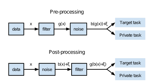
Figure 2: Preprocessing and postprocessing approaches to differentially private minimax filtering.

Minimax filters can be made locally differentially private using the additive noise mechanism (79) in the signal chain of filtering. The paper proposes two approaches. In the preprocessing approach, filtering is performed first and is followed by perturbation. In the postprocessing approach, perturbation is applied first and is followed by filtering. Note that preprocessing and postprocessing approaches are similar to output perturbation and input perturbation in Sarwate and Chaudhuri (2013). Fig. 2 shows the signal chains of the two approaches. In preprocessing, the original feature $x$ is first filtered by $g(x)$, and then made differential private by a bounding function and perturbation $b(g(x))+\xi$. In postprocessing, the original feature $x$ is first made differentially private by a bounding function and perturbation $b(x)+\xi$ followed by filtering $g(b(x)+\xi)$. By adding an appropriate amount of noise, both approaches can be made $\epsilon$-differentially private regardless of data distribution. However, when the noisy mechanism is used in conjunction with a minimax filter which is dependent on data distribution $P(x,y,z)$, preprocessing and postprocessing approaches have different effects that depend on the distribution.

A scenario when preprocessing is preferable to postprocessing is as follows. For the convenience of explanation, let’s assume that subject identification is the private task. Let $y(x)$ be the subject identity label of sample $x$ and let $z(x)$ be the target label of sample $x$ for any target task. Define between-subject diameter as the max distance of two samples $x,x^{\prime}$ from different subjects that have the same target label:

$$S_{b}\triangleq\max_{x,x^{\prime}\in\mathcal{X}}\|x-x^{\prime}\|\;\;\;\mathrm{s.t.}\;\;\;y(x)\neq y(x^{\prime}),\;z(x)=z(x^{\prime}).$$ (83)

Similarly, define within-subject diameter as the max distance of two samples $x,x^{\prime}$ from the same subject that have different target labels:

$$S_{w}\triangleq\max_{x,x^{\prime}\in\mathcal{X}}\|x-x^{\prime}\|\;\;\;\mathrm{s.t.}\;\;\;y(x)=y(x^{\prime}),\;z(x)\neq z(x^{\prime}).$$ (84)

Also for the purpose of explanation, assume that the filter $g$ is an orthogonal projection onto a lower-dimensional Euclidean space. For a given data set $\mathcal{X}$, if the between-subject diameter is larger than the within-subject diameter ($S_{b}>S_{w}$) in the original feature space (Fig. 3a), then minimax filtering can potentially reduce the diameter $S(g)=\max_{x,x^{\prime}}\|g(x)-g(x^{\prime})\|$ significantly. This translates to less amount of noise required to achieve the same $\epsilon$-privacy than the amount of noise required before filtering, as the data diameter has shrunk. This will result in better utility of the preprocessing approach over the postprocessing approach where noise is added before filtering. From the same reasoning, if the opposite is true ($S_{w}>S_{b}$) (Fig. 3b), then the diameter $S(g)$ after minimax filtering does not change much, and the preprocessing approach may not offer much benefit over the postprocessing approach. However, there are still other differences between the two approaches. This paper assumes that the training data are public information and their privacy is not the primary concern unlike the privacy of test data. However, if we begin to consider the privacy of training data as well, then one should be aware that the learned filters can leak private information, analogous to how the PCA components can leak information about training data (Chaudhuri et al., 2012), and that the filters also need to be sanitized before release. The postprocessing approach makes the whole process simpler. In this case, after each data owner perturbs the data by herself, any subsequent postprocessing, whether it is the process of applying pretrained filters or the process of training minimax filters, does not worsen differential privacy guarantees (Dwork et al., 2014), and therefore the postprocessing approach is a safer choice when the data owners cannot trust the entity that collects training data.

Figure 3: Two example data distributions which have the same data diameter before filtering but have different diameters after filtering. a. an example where between-subject diameter (83) is large. b. an example where within-subject diameter (84) is large.

6 Experiments

In this section, the algorithms proposed in the paper are evaluated using three real-world data sets: face data for gender/expression classification, speech data for emotion classification, and motion data for activity classification. Firstly, minimax filters are compared with non-minimax methods in terms of privacy breach vs utility as measured by accuracy of private and target tasks classifiers on test data. Secondly, noisy minimax filters are tested under various conditions using the same data sets.

6.1 Methods

Filters. The following minimax and non-minimax filters are compared.

• Rand: random subspace projection with $g(x;U)=U^{T}x$, where $U$ is a random full rank $D\times d$ matrix.

• PCA: principal component analysis with $g(x;U)=U^{T}x$, where $U$ is the eigenvectors corresponding to $d$ largest eigenvalues of $\mathrm{Cov}(x)$.

• PPLS: private partial least squares, using Algorithm 1 from Enev et al. (2012).

• DDD: discriminately decreasing discriminability (DDD) from Whitehill and Movellan (2012) with a mask-type filter from the code.

• Minimax 1: linear filter $g(x;U)=U^{T}x$ where $U$ is computed from Alg. (1).

• Minimax 2: nonlinear filter $g(x)$ from a two-layer sigmoid neural network with of hidden nodes of $20$ and $10$, computed from Alg. 1.

Remarks. DDD requires analytical solutions to eigenvalue problems which are unavailable for multiclass problems, and is used only in the binary problem with the face database. Also, DDD uses a mask-type filter in the codes, and the dimension $d$ is same as the image size. The dimension $d$ is also irrelevant to nonlinear Minimax filter 2 since it does not use linear dimensionality reduction. The nonlinear filter is pretrained as a stacked denoising autoencoders (Vincent et al., 2008) followed by supervised backpropagation with the target task. Classifier/loss. For all experiments, binary or multinomial logistic regression is used a classifier for both utility and privacy risks, where the loss $l(h(g(x;u);v),y)$ is the negative log-likelihood with regularization:

$$l=-v(y)^{T}g(x;u)+\log(\sum_{k=1}^{K}e^{v(k)^{T}g(x;u)})+\frac{\lambda}{2}\sum_{k=1}^{K}\|v(k)\|^{2}$$ (85)

where $K$ is the number of classes. The regularization coefficient was $\lambda=10^{-6}$ and the utility-privacy tradeoff coefficient was $\rho=10$. The main iteration in Alg. 1 was stopped when the progress was slow, which was between $T=20-200$.

6.2 Data sets

Gender/expression classification from face: The GENKI database (Whitehill and Movellan, 2012) consists of face images with varying poses and facial expressions. The original data set is used unchanged, which has $N=1740$ training images (50% male and 50% female; 50% smile and 50% non-smile). The test set has 100 images (50 males and 50 females; 50 smiling and 50 non-smiling) not overlapping with the training set. The dimensionality of the original data is $D=256$, and the filters are tested with $d=10,20,50,100$. The data set has gender and expression labels but no subject label. Consequently, gender classification is used as the private task and expression classification is used as the target task.

Emotion classification from speech: The ENTERFACE database (Martin et al., 2006) is an audiovisual emotion database of 43 speakers from 14 nations reading predefined English sentences in six induced emotions. From the raw speech signals sampled in 48 KHz, MFCC coefficients are computed using 20 ms windows with 50% overlap and 13 Mel-frequency bands. The mean, max, min, and standard deviation of the MFCC coefficients over the duration of each sentence are computed, resulting in $N=427$ samples of $D=52$ dimensional feature vectors from $S=43$ subjects. Each subject’s samples are randomly split to generate training (80%) and test (20%) sets. Average test accuracy over 10 such trials is reported. Filters are tested with $d=10,20,30,40$. The target task is the binary classification of ‘happy’ and ‘non-happy’ emotions from speech, and the privacy task is the multiclass $(S=43)$ subject classification.

Activity classification from motion: The UCI Human Activity Recognition (HAR) data set (Anguita et al., 2012) is a collection of motion sensor data on a smartphone by 30 subjects performing six activities (walking, walking upstairs, walking downstairs, sitting, standing, laying). Various time and frequency domain variables are extracted from the signal, resulting in $N=10299$ samples of $D=561$ dimensional features from $30$ subjects which are used unchanged. Out of 30 subjects, 15 subjects are chosen randomly. For each domain, each subject’s samples are randomly split to generate training (50%) and test (50%) sets. At each trial, the subjects and the training/test sets are randomized, and the average test accuracy over 10 such trials is reported. Filters with dimensions $d=10,20,50,100$ are used. The target task is the multiclass ($C=6$) classification of activity, and the privacy task is the multiclass $(S=15)$ subject classification.

6.3 Result 1: Minimax filters

Before any filter is applied, the accuracy of the target tasks with raw data is 0.90 (GENKI), 0.84 (ENTERFACE), and 0.97 (HAR). On the other hand, the accuracy of the private tasks with raw data is 0.90 (GENKI), 0.62 (ENTERFACE), and 0.70 (HAR). The high accuracy of the private tasks (considering the chance level accuracy of 0.5 (GENKI), 0.02 (ENTERFACE), and 0.067 (HAR)) demonstrates that an adversary can accurately infer private variables such as gender and identity from raw data if no filter is used. A simple defense against inference attack is to perform dimensionality reduction on the original data, such as Rand and PCA projections. As the dimensionality $d$ decreases from the original value $D$ towards zero, one can expect both the private and the target accuracy to decrease toward the chance level. This trend is indeed the case with both the non-private (Rand,PCA) and the private (PPLS,DDD,Minimax) filters used in the paper. Therefore these filters are evaluated at several different values of the dimensionality $d$ to make fine-grained comparisons of utility-privacy.

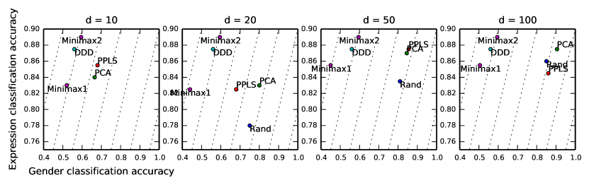
Figure 4: GENKI: Expression classification vs and gender classification from faces.

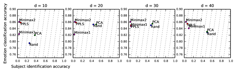
Figure 5: ENTERFACE: Emotion classification vs and subject identification from speech.

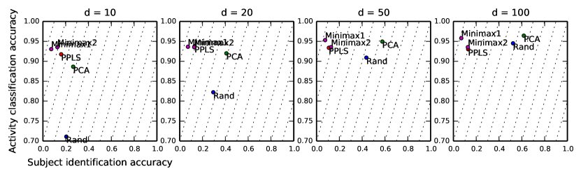
Figure 6: HAR: Activity classification vs subject identification from motion.

Fig. 4 shows the test accuracy with GENKI. The dotted lines are level sets of utility-privacy tradeoff (i.e., target task accuracy - private task accuracy) shown for reference. Minimax 2 achieves the best utility (i.e., most accurate expression classification) and Minimax 1 (linear) achieves the best privacy (i.e., least accurate gender classification). For all dimensions $d$, Minimax 1 achieves the best utility-privacy compromise (i.e., closest to the top-left corner of the plot), with Minimax 2 and DDD performing similarly. In terms of private task accuracy, Minimax 1 achieves almost the chance level accuracy (0.5), which implies a strong privacy preservation. DDD comes close to Minimax 1, while another private method PPLS is not very successful in preventing the inference of the private variable. As expected, non-private methods Rand and PCA also do not reduce the privacy task accuracy. As dimension $d$ increases from 10 to 100, the accuracy of both the target and the private tasks increase (toward the top-right corner of the plot) for PPLS, PCA and Rand, but the value of utility-privacy tradeoff (i.e., target task accuracy - private task accuracy) remains relatively similar even though $d$ changes. Note that $d$ is irrelevant to Minimax 2 and DDD.

Fig. 5 shows the test accuracy of ENTERFACE. Minimax 2 achieves the best utility (i.e., most accurate emotion classification) and the best privacy (i.e., least accurate subject classification) at the same time. PPLS performs well in this task; its private and target task accuracy is close to those of Minimax 2. The private task accuracy of Minimax 2 is near the chance level ($1/S=0.02$) compared to $0.4-0.5$ of non-private methods, suggesting that seemingly harmless statistics (mean, max, min, s.d. of MFCC) are quite susceptible to identification attacks if no privacy mechanism is used. Similar to GENKI, the accuracy of both the target and the private tasks increases with the dimension $d$ for PCA and Rand, and the value of utility-privacy tradeoff remains similar regardless of $d$.

Fig. 6 shows the test accuracy of HAR. Minimax 1 achieves the best utility (i.e., most accurate activity recognition) and the best privacy (i.e., least accurate subject classification), while Minimax 2 and PPLS performs similarly well. The private task accuracy of Minimax 1 is lower than others close to the chance level ($1/S=0.067$). The figure also shows that motion data are susceptible ($0.2-0.7$) to identification attacks when no privacy mechanism is used. For all dimensions $d$, Minimax 1 achieves the best compromise of all methods similar to previous experiments. Also the accuracy of both the target and the private tasks roughly increases with $d$ for PCA and Rand, but the value of utility-privacy tradeoff remains similar.

6.4 Result 2: Noisy minimax filters

The same data sets from the previous section are used to demonstrate the effect of noisy mechanism on minimax filters. Four types of noisy filters are compared: PCA-pre, PCA-post, Minimax-pre, and Minimax-post. PCA is chosen as a non-minimax reference filter which preserves the original signal the best in the least mean-squared-error sense. PCA-pre/post means that PCA is applied before/after the perturbation similarly to Minimax-pre/post from Fig. 2. For Minimax-pre/post, a linear filter of the same dimension $d$ as PCA-pre/post is used. Tests are performed for the same ranges of dimension $d$ as in Sec 6.3. The results for $d=20$ with all three data sets are summarized in Fig. 7. Results for different dimensions show similar trends and are summarized in Fig. 8. Optimization of (7) is done similarly to the previous section. All tests are repeated 10 times for different noise samples of (80), for each of 10 random training/test splits.

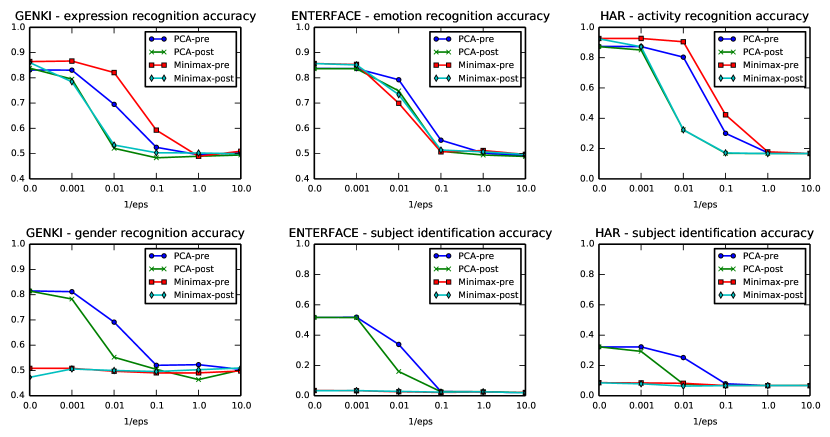
Figure 7: Impact of four noisy filters (PCA-pre/post and Minimax-pre/post) on the accuracy of target and private tasks for three data sets (GENKI, ENTERFACE, HAR), over the range of $\epsilon^{-1}=\{0,10^{-3},10^{-2},10^{-1},10^{0},10^{1}\}$. Top row is the target task accuracy (higher the better) and bottom row is the private task accuracy (lower the better.) Minimax-pre/post can limit the accuracy of inference attack (bottom row) to almost chance levels regardless of the value of $\epsilon$, while PCA-pre/post requires a significantly high $\epsilon$ to prevent inference attacks which also destroy the utility.

Fig. 7 shows the following results. Firstly, within each plot, increasing the privacy level from left ($\epsilon^{-1}\mathtt{=}0$) to right ($\epsilon^{-1}\mathtt{=}10$) lowers the accuracy of both target and private tasks for all filter types and data sets, which is intuitively correct. Secondly, target task accuracy (top row) shows that the four filters are equally accurate with no noise ($\epsilon^{-1}\mathtt{=}0$), with Minimax-pre/post slightly more accurate than PCA-pre/post. This observation is consistent with the results in Sec. 6.3. In GENKI and HAR, preprocessing is better than postprocessing for both PCA and Minimax, and Minimax-pre performs the best. In ENTERFACE, preprocessing and postprocessing approaches perform similarly, and all four filters is perform similarly on the target task. This result may be ascribed to the discussion of different data distribution in Sec. 5.2. Thirdly, and most importantly, private task accuracy (bottom row) is quite different between Minimax-pre/post and non-minimax PCA-pre/post. For both Minimax-pre and Minimax-post, the private task accuracy is almost as low as the chance accuracy of each data set (0.5, 0.03, 0.07) regardless of the noise level $\epsilon$. This demonstrates that minimax filter can prevent inference attacks with little help of noise. In contrast, the non-minimax filters (PCA-pre/post) allow an adversary to infer private variables quite accurately (0.8, 0.5, 0.3) when no noise is used. Preventing such attacks for non-minimax filters requires a significant amount of additive noise (e.g., $\epsilon^{-1}{\geq}0.1$) which destroys the utility of data. These results show that differentially privacy is indeed different from privacy against inference attacks and the combination of two methods is beneficial.

7 Conclusion

This work presents a new learning-based mechanism for preventing inference attacks on continuous and high-dimensional data. In this mechanism, a filter transforms continuous and high-dimensional raw features to dimensionality-reduced representations of data. After filtering, information on target tasks remains but information on identifying or sensitive attributes is removed which makes it difficult for an adversary to accurately infer such attributes from the released filtered output. Minimax filters are designed to achieve the optimal utility-privacy tradeoff in terms of expected risks. The paper proves that a filter learned from empirical risks is not far from an ideal filter that is learned from expected risks as the number of samples increases. This property and its dependency on the task make this mechanism quite different from previous mechanisms, including syntactic anonymization and differential privacy. Algorithms for finding minimax filters are presented and evaluated on real-world data sets to show its practical usages. Experiments show that publicly available multisubject data sets are surprisingly susceptible to subject identification attacks, and that even simple linear minimax filters can reduce the privacy risks close to chance level without sacrificing target task accuracy by much.

This work also presents preprocessing and postprocessing approaches to combine minimax privacy and differential privacy. While differential privacy has become a popular criterion of privacy loss, it is not without limitations, in particular against inference attacks as empirically demonstrated in the paper. This leaves room for development of new mechanisms such as the noisy minimax filter presented in the paper, which aims to achieve high on-average utility and protection against inference attacks, and a formal privacy guarantee to a degree. The results from experiments encourage further research on potential benefits of combining different notions and mechanisms of privacy, which is left as future work.

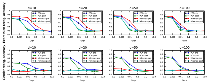
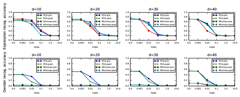
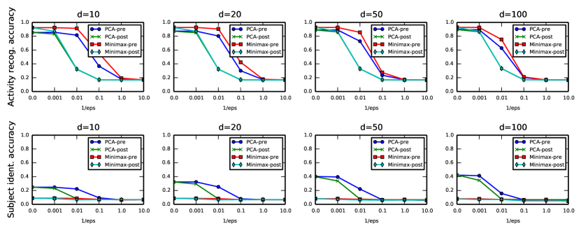
Figure 8: The full result of the performance noisy filters (PCA-pre/post and Minimax-pre/post) on the accuracy of target and private tasks on three data sets: GENKI (1st & 2nd row), ENTERFACE (3rd & 4th row), HAR (5th & 6th row).

References

- Alvim et al. (2012) Mário S Alvim, Miguel E Andrés, Konstantinos Chatzikokolakis, Pierpaolo Degano, and Catuscia Palamidessi. Differential privacy: on the trade-off between utility and information leakage. In Formal Aspects of Security and Trust, pages 39–54. Springer, 2012.
- Anguita et al. (2012) Davide Anguita, Alessandro Ghio, Luca Oneto, Xavier Parra, and Jorge L Reyes-Ortiz. Human activity recognition on smartphones using a multiclass hardware-friendly support vector machine. In Ambient assisted living and home care, pages 216–223. Springer, 2012.
- Brickell and Shmatikov (2008) Justin Brickell and Vitaly Shmatikov. The cost of privacy: destruction of data-mining utility in anonymized data publishing. In Proceedings of the 14th ACM SIGKDD international conference on Knowledge discovery and data mining, pages 70–78. ACM, 2008.
- Chaudhuri et al. (2012) Kamalika Chaudhuri, Anand Sarwate, and Kaushik Sinha. Near-optimal differentially private principal components. In Advances in Neural Information Processing Systems, pages 989–997, 2012.
- Clifton and Tassa (2013) Chris Clifton and Tamir Tassa. On syntactic anonymity and differential privacy. Transactions on Data Privacy, 6(2):161–183, 2013.
- Cormode (2011) Graham Cormode. Personal privacy vs population privacy: learning to attack anonymization. In Proceedings of the 17th ACM SIGKDD international conference on Knowledge discovery and data mining, pages 1253–1261. ACM, 2011.
- Danskin (1967) John M Danskin. The theory of max-min and its application to weapons allocation problems. Springer, 1967.
- du Pin Calmon and Fawaz (2012) Flávio du Pin Calmon and Nadia Fawaz. Privacy against statistical inference. In Communication, Control, and Computing (Allerton), 2012 50th Annual Allerton Conference on, pages 1401–1408. IEEE, 2012.
- Duchi et al. (2013) John C Duchi, Michael I Jordan, and Martin J Wainwright. Local privacy and statistical minimax rates. In Foundations of Computer Science (FOCS), 2013 IEEE 54th Annual Symposium on, pages 429–438. IEEE, 2013.
- Dwork (2006) Cynthia Dwork. Differential privacy. In Automata, languages and programming, pages 1–12. Springer, 2006.
- Dwork and Nissim (2004) Cynthia Dwork and Kobbi Nissim. Privacy-Preserving Data Mining on Vertically Partitioned Databases. In Proc. CRYPTO. Springer, 2004.
- Dwork et al. (2006) Cynthia Dwork, Frank McSherry, Kobbi Nissim, and Adam Smith. Calibrating noise to sensitivity in private data analysis. In Theory of Cryptography, pages 265–284. Springer, 2006.
- Dwork et al. (2014) Cynthia Dwork, Aaron Roth, et al. The algorithmic foundations of differential privacy. Foundations and Trends in Theoretical Computer Science, 9(3-4):211–407, 2014.
- Enev et al. (2012) Miro Enev, Jaeyeon Jung, Liefeng Bo, Xiaofeng Ren, and Tadayoshi Kohno. Sensorsift: balancing sensor data privacy and utility in automated face understanding. In Proceedings of the 28th Annual Computer Security Applications Conference, pages 149–158. ACM, 2012.
- Fung et al. (2010) Benjamin Fung, Ke Wang, Rui Chen, and Philip S Yu. Privacy-preserving data publishing: A survey of recent developments. ACM Comp. Surveys (CSUR), 42(4):14, 2010.
- Ghosh et al. (2009) Arpita Ghosh, Tim Roughgarden, and Mukund Sundararajan. Universally utility-maximizing privacy mechanisms. In Proceedings of the forty-first annual ACM symposium on Theory of computing, pages 351–360. ACM, 2009.
- Goodfellow et al. (2014) Ian Goodfellow, Jean Pouget-Abadie, Mehdi Mirza, Bing Xu, David Warde-Farley, Sherjil Ozair, Aaron Courville, and Yoshua Bengio. Generative adversarial nets. In Advances in Neural Information Processing Systems, pages 2672–2680, 2014.
- Hall et al. (2013) Rob Hall, Alessandro Rinaldo, and Larry Wasserman. Differential privacy for functions and functional data. Journal of Machine Learning Research, 14(Feb):703–727, 2013.
- Hamm (2015) Jihun Hamm. Preserving privacy of continuous high-dimensional data with minimax filters. In Proceedings of the Eighteenth International Conference on Artificial Intelligence and Statistics (AISTATS), 2015.
- Hamm (2017) Jihun Hamm. Enhancing utility and privacy with noisy minimax filters. In Acoustics, Speech and Signal Processing (ICASSP), 2017 IEEE International Conference on, pages 6389–6393. IEEE, 2017.
- Hamm et al. (2016) Jihun Hamm, Paul Cao, and Mikhail Belkin. Learning privately from multiparty data. In Proceedings of The 33rd International Conference on Machine Learning (ICML), pages 555–563, 2016.
- Iyengar (2002) Vijay S Iyengar. Transforming data to satisfy privacy constraints. In Proceedings of the eighth ACM SIGKDD international conference on Knowledge discovery and data mining, pages 279–288. ACM, 2002.
- Kasiviswanathan et al. (2011) Shiva Prasad Kasiviswanathan, Homin K Lee, Kobbi Nissim, Sofya Raskhodnikova, and Adam Smith. What can we learn privately? SIAM Journal on Computing, 40(3):793–826, 2011.
- Kifer (2009) Daniel Kifer. Attacks on privacy and definetti’s theorem. In Proceedings of the 2009 ACM SIGMOD International Conference on Management of data, pages 127–138. ACM, 2009.
- Kiwiel (1987) Krzysztof C Kiwiel. A direct method of linearization for continuous minimax problems. Journal of optimization theory and applications, 55(2):271–287, 1987.
- Krause and Horvitz (2008) Andreas Krause and Eric Horvitz. A utility-theoretic approach to privacy and personalization. In AAAI, volume 8, pages 1181–1188, 2008.
- Li and Li (2009) Tiancheng Li and Ninghui Li. On the tradeoff between privacy and utility in data publishing. In Proceedings of the 15th ACM SIGKDD international conference on Knowledge discovery and data mining, pages 517–526. ACM, 2009.
- Machanavajjhala et al. (2007) Ashwin Machanavajjhala, Daniel Kifer, Johannes Gehrke, and Muthuramakrishnan Venkitasubramaniam. l-diversity: Privacy beyond k-anonymity. ACM Transactions on Knowledge Discovery from Data (TKDD), 1(1):3, 2007.
- Martin et al. (2006) Olivier Martin, Irene Kotsia, Benoit Macq, and Ioannis Pitas. The enterface´05 audio-visual emotion database. In Data Engineering Workshops, 2006. Proceedings. 22nd International Conference on, pages 8–8. IEEE, 2006.
- Narayanan and Shmatikov (2008) Arvind Narayanan and Vitaly Shmatikov. Robust de-anonymization of large sparse datasets. In Security and Privacy, 2008. SP 2008. IEEE Symposium on, pages 111–125. IEEE, 2008.
- Nedić and Ozdaglar (2009) Angelia Nedić and Asuman Ozdaglar. Subgradient methods for saddle-point problems. Journal of optimization theory and applications, 142(1):205–228, 2009.
- Newton et al. (2005) Elaine M Newton, Latanya Sweeney, and Bradley Malin. Preserving privacy by de-identifying face images. Knowledge and Data Engineering, IEEE Transactions on, 17(2):232–243, 2005.
- Panin (1981) VM Panin. Linearization method for continuous min-max problem. Cybernetics and Systems Analysis, 17(2):239–243, 1981.
- Rastogi and Nath (2010) Vibhor Rastogi and Suman Nath. Differentially private aggregation of distributed time-series with transformation and encryption. In Proceedings of the 2010 ACM SIGMOD International Conference on Management of data, pages 735–746. ACM, 2010.
- Rebollo-Monedero et al. (2010) David Rebollo-Monedero, Jordi Forne, and Josep Domingo-Ferrer. From t-closeness-like privacy to postrandomization via information theory. Knowledge and Data Engineering, IEEE Transactions on, 22(11):1623–1636, 2010.
- Rustem and Howe (2009) Berc Rustem and Melendres Howe. Algorithms for worst-case design and applications to risk management. Princeton University Press, 2009.
- Sankar et al. (2010) Lalitha Sankar, Raj Rajagopalan, and Vincent Poor. An information-theoretic approach to privacy. In Communication, Control, and Computing (Allerton), 2010 48th Annual Allerton Conference on, pages 1220–1227. IEEE, 2010.
- Sarwate and Chaudhuri (2013) Anand Sarwate and Kamalika Chaudhuri. Signal processing and machine learning with differential privacy: Algorithms and challenges for continuous data. Signal Processing Magazine, IEEE, 30(5):86–94, 2013.
- Shalev-Shwartz and Ben-David (2014) Shai Shalev-Shwartz and Shai Ben-David. Understanding Machine Learning: From Theory to Algorithms. Cambridge University Press, New York, NY, USA, 2014. ISBN 1107057132, 9781107057135.
- Smith (2011) Adam Smith. Privacy-preserving statistical estimation with optimal convergence rates. In Proceedings of the forty-third annual ACM symposium on Theory of computing, pages 813–822. ACM, 2011.
- Sweeney (2002) Latanya Sweeney. k-anonymity: A model for protecting privacy. International Journal of Uncertainty, Fuzziness and Knowledge-Based Systems, 10(05):557–570, 2002.
- Vincent et al. (2008) Pascal Vincent, Hugo Larochelle, Yoshua Bengio, and Pierre-Antoine Manzagol. Extracting and composing robust features with denoising autoencoders. In Proceedings of ICML, pages 1096–1103. ACM, 2008.
- Whitehill and Movellan (2012) Jacob Whitehill and Javier Movellan. Discriminately decreasing discriminability with learned image filters. In Computer Vision and Pattern Recognition (CVPR), 2012 IEEE Conference on, pages 2488–2495. IEEE, 2012.
- Xiao et al. (2011) Xiaokui Xiao, Guozhang Wang, and Johannes Gehrke. Differential privacy via wavelet transforms. IEEE Transactions on Knowledge and Data Engineering, 23(8):1200–1214, 2011.
- Xu et al. (2017) Ke Xu, Tongyi Cao, Swair Shah, Crystal Maung, and Haim Schweitzer. Cleaning the null space: A privacy mechanism for predictors. In AAAI, pages 2789–2795, 2017.