Non–Resonant Two–Photon Transitions in Length and Velocity Gauges

Abstract

We reexamine the invariance of two-photon transition matrix elements and corresponding two-photon Rabi frequencies under the “gauge” transformation from the length to the velocity gauge. It is shown that gauge invariance, in the most general sense, only holds at exact resonance, for both one-color as well as two-color absorption. The arguments leading to this conclusion are supported by analytic calculations which express the matrix elements in terms of hypergeometric functions, and ramified by a “master identity” which is fulfilled by off-diagonal matrix elements of the Schrödinger propagator under a the transformation from the velocity to the length gauge. The study of the gauge dependence of atomic processes highlights subtle connections between the concept of asymptotic states, the gauge transformation of the wave function, and infinitesimal damping parameters for perturbations and interaction Hamiltonians that switch off the terms in the infinite past and future [of the form $\exp(-\epsilon|t|)$]. We include a pertinent discussion.

I Introduction

A priori, the description of any dynamic process in atomic physics should be gauge invariant. Yet, there is a caveat. Namely, one usually calculates atomic transitions using wave functions obtained from the solution of the unperturbed Schrödinger equation, and ignores both the gauge transformation of the wave function as well as the fact that the physical interpretation of the wave function changes under a gauge transformation from the velocity to the length gauge. Lamb Lamb (1952) has shown that if one insists on using ordinary Schrödinger wave functions in off-resonant one-photon transition matrix elements, then the length gauge form has to be used for the laser field. Here, we refer to off-resonant transitions as those where the frequency of the incident radiation is not exactly equal to the resonance frequency of the atom; generalized to two-photon transitions, this implies that the sum frequency of the two photons does not exact match the energy (frequency) difference of the ground and excited level.

For off-resonant two-photon transitions, one might think that the transition matrix element could be equal in the length and velocity gauges if all possible intermediate, virtual states are included in the calculation. Here, inspired by Refs. Bassani et al. (1977); Kobe (1978); Schlicher et al. (1984), we aim to reinvestigate the status of the gauge invariance of two-photon transition matrix elements (“length” versus “velocity” gauges). Note that invariance under the change from the “length” to the “velocity” gauges implies that the gauge transformation of the wave function is ignored (we also refer to the invariance of matrix elements under the neglect of the wave function transformation and under the neglect of any necessary reinterpretation of physical operators as the “extended gauge invariance”). In Refs. Power and Thirunamachandran (1975, 1978), the two-photon transition matrix element has been examined without any additional condition enforced upon the laser frequency; the laser might be off-resonant or on resonance. As is explained below, the arguments given in Refs. Power and Thirunamachandran (1975, 1978) appear to be applicable only at exact resonance. The role of the intermediate, virtual quantum states in the gauge invariance will be analyzed here in terms of general identities, applicable to various physical processes. Second, from a conceptual point of view, the role of the gauge transformation of the wave function and the concomitant change in its interpretation appears to profit from further explanatory remarks beyond the problem at hand.

The subject matter of this article is rather basic quantum mechanics, supplemented with explicit analytic results for the length and velocity forms of the $1S$–$2S$ two-photon transition matrix element in hydrogen. We start by investigating gauge transformations and physical interpretations of operators in Sec. II, before reexamining the “gauge invariance” of the ac Stark shift under a change of the interaction Hamiltonian from the length to the velocity form (Sec. III). Here, “gauge invariance” has to taken with a grain of salt; the invariance of the theoretical expressions for the ac Stark shift holds even if the mandatory gauge transformation of the wave function is neglected, a fact on which we comment in Sec. IV. In Sec. III, we shall examine, based on explicit analytic and numerical calculations, the behavior of a typical two-photon transition matrix element (namely, of the $1S$–$2S$ two-photon transition in hydrogen) off resonance. We aim to show that the inclusion of the intermediate states does not solve the problem of gauge invariance, but the gauge dependence is due to a change in the physical interpretation of the wave function under the presence of a nonvanishing vector potential. The physically correct result for the transition rate off resonance is obtained in the length gauge.

II Gauge Transformation and Physical Interpretations

In order to illustrate that gauge transformations can change the physical interpretation of operators, let us start from a trivial example. We consider a wave function $\psi(\vec{r})=1/\sqrt{V}$ where $V$ is the normalization volume; it describes a particle at rest. A unitary “gauge” transformation of the form

$$\psi(\vec{r})\to\exp\left(\frac{{\mathrm{i}}}{\hbar}\vec{p}_{0}\cdot\vec{r}\right)\,\psi(\vec{r})$$ (1)

is applied. The momentum operator in the free Hamiltonian $H=\vec{p}^{\,2}/(2m)$, with $\vec{p}=-{\mathrm{i}}\vec{\nabla}$, transforms as

$$\vec{p}\to{\mathrm{e}}^{\frac{{\mathrm{i}}}{\hbar}\vec{p}_{0}\cdot\vec{r}}\;\vec{p}\;{\mathrm{e}}^{-\frac{{\mathrm{i}}}{\hbar}\vec{p}_{0}\cdot\vec{r}}=\vec{p}-\vec{p}_{0}\,.$$ (2)

The gauge-transformed Hamiltonian thus reads as $H^{\prime}=(\vec{p}-\vec{p}_{0})^{2}/(2m)$, and the interpretation of the momentum operator $\vec{p}=-{\mathrm{i}}\hbar\vec{\nabla}$ has changed: Namely, the kinetic momentum operator no longer is $\vec{p}$, but $\vec{p}-\vec{p}_{0}$. Indeed, $\vec{p}_{\rm kin}=\vec{p}-\vec{p}_{0}$ is the conjugate variable of the position operator $\vec{r}$ (see also the Appendix of Ref. Jentschura and Noble (2013)).

A similar situation is encountered in electrodynamics Reiss . The time-dependent wave function receives a unitary gauge transform,

$$\psi(t,\vec{r})\to{\mathrm{e}}^{\frac{{\mathrm{i}}}{\hbar}e\Lambda(t,\vec{r})}\,\psi(t,\vec{r})\,.$$ (3)

The momentum operator transforms as

$$\vec{p}\to \;{\mathrm{e}}^{\frac{{\mathrm{i}}}{\hbar}e\Lambda(t,\vec{r})}\,\vec{p}\,{\mathrm{e}}^{-\frac{{\mathrm{i}}}{\hbar}e\Lambda(t,\vec{r})}\,\to\vec{p}-e\vec{\nabla}\Lambda(t,\vec{r})\,,$$ (4)

where $e$ is the electron charge. The following Hamiltonian describes the atom-electromagnetic field dynamical system consisting of an electron coupled to a vector potential $\vec{A}$, in the binding (Coulomb) potential $\Phi$,

$$H=\frac{(\vec{p}-e\,\vec{A})^{2}}{2m}+e\Phi\,.$$ (5)

The product $e\Phi$ of electron charge and binding scalar potential is often denoted as $V$, because it acts as a potential term in the Hamiltonian. Typicall, the vector potential $\vec{A}$ describes a laser. The unitary gauge transformation, applied to $H$, leads to the transformed Hamiltonian $\widetilde{H}$,

$$\widetilde{H}={\mathrm{e}}^{\frac{{\mathrm{i}}}{\hbar}e\Lambda(t,\vec{r})}\,H\,{\mathrm{e}}^{-\frac{{\mathrm{i}}}{\hbar}e\Lambda(t,\vec{r})}=\frac{(\vec{p}-e\,\vec{A}^{\prime})^{2}}{2m}+e\Phi\,,$$ (6)

where $\vec{A}^{\prime}=\vec{A}+\vec{\nabla}\Lambda$ is the gauge-transformed vector potential. Conversely, for $\vec{A}=\vec{0}$, and $\vec{A}^{\prime}=\vec{\nabla}\Lambda\neq\vec{0}$, one asserts that the interpretation of the momentum operator $\vec{p}=-{\mathrm{i}}\hbar\vec{\nabla}$ changes; it no longer describes the kinetic momentum. The place of the latter is taken by the conjugate variable of position, namely, $\vec{p}_{\rm kin}=\vec{p}-e\,\vec{A}^{\prime}$.

However, under the gauge transformation, the physical interpretation of the Hamiltonian also changes. A priori, the Hamiltonian $H$ is equal to the the time derivative operator ${\mathrm{i}}\hbar\partial_{t}$. After the gauge transformation, it is equal to a unitarily transformed time derivative operator,

$${\mathrm{i}}\hbar\partial_{t}\to{\mathrm{e}}^{\frac{{\mathrm{i}}}{\hbar}e\Lambda(t,\vec{r})}\,({\mathrm{i}}\hbar\partial_{t})\,{\mathrm{e}}^{-\frac{{\mathrm{i}}}{\hbar}e\Lambda(t,\vec{r})}\to{\mathrm{i}}\hbar\partial_{t}+e\partial_{t}\Lambda(t,\vec{r})\,.$$ (7)

The new time derivative operator is thus obtained by setting equal the unitarily transformed Hamiltonian and the unitarily transformed time derivative operator, and reads as

$$H^{\prime}=\widetilde{H}-e\partial_{t}\Lambda=\frac{(\vec{p}-\vec{A}^{\prime})^{2}}{2m}+e\,\Phi^{\prime}\,,$$ (8)

where $\Phi^{\prime}=\Phi-\partial_{t}\Lambda$ is the gauge-transformed scalar potential.

From the above derivation, which in principle recalls well-known facts, it is immediately obvious that the gauge-transformed Hamiltonian $H^{\prime}$ cannot be obtained from $H$ by a unitary transformation. Conversely, the unitarily transformed $\widetilde{H}$ cannot be interpreted any more as the time derivative operator when acting on the gauge-transformed wave function.

In order to fix ideas, it is useful to examine the velocity-gauge one-photon transition matrix element $\mathcal{M}_{v}$,

$$\mathcal{M}_{v}= \;\left<\phi_{f}\left|-e\,\frac{\vec{A}\cdot\vec{p}}{m}+\frac{e^{2}\vec{A}^{\,2}}{2m}\right|\phi_{i}\right>$$

$$\to \;\left<\phi_{f}\left|-e\,\frac{\vec{A}\cdot\vec{p}}{m}\right|\phi_{i}\right>=\left<\phi_{f}\left|-e\,\frac{{\mathrm{i}}}{\hbar}\,\vec{A}\cdot[H,\vec{r}]\right|\phi_{i}\right>$$

$$= \;-e\,\frac{{\mathrm{i}}}{\hbar}(E_{f}-E_{i})\,\left<\phi_{f}\left|\vec{A}\cdot\vec{r}\right|\phi_{i}\right>$$ (9)

of an initial atomic state $|\phi_{i}\rangle$ and a final state $|\phi_{f}\rangle$. [We have made the dipole approximation $\vec{A}=\vec{A}(t)$ and assumed that the seagull term $e^{2}\vec{A}^{\,2}/(2m)$ does not contribute because of the angular symmetry of the initial and final states involved in the dipole transition.] In view of the identity $\vec{E}=-\partial_{t}\vec{A}\to{\mathrm{i}}\omega\,\vec{A}$, the length-gauge one-photon matrix elements $\mathcal{M}_{\ell}$ is related to its velocity-gauge counterpart $\mathcal{M}_{v}$ as follows,

$$\mathcal{M}_{\ell}= \;\left<\phi_{f}\left|-e\,\vec{E}\cdot\vec{r}\right|\phi_{i}\right>$$

$$\to \;-{\mathrm{i}}\omega\,\frac{e}{m}\,\left<\phi_{f}\left|\vec{A}\cdot\vec{r}\right|\phi_{i}\right>=\frac{\hbar\omega}{E_{f}-E_{i}}\,\mathcal{M}_{v}\,.$$ (10)

The velocity-gauge expression $\mathcal{M}_{v}$ differs from its length-gauge counterpart $\mathcal{M}_{\ell}$ by an additional factor $(E_{f}-E_{i})/\omega$. Hence, in a remark on p. 268 of Ref. Lamb (1952), Lamb observed that the physical interpretation of the wave function is preserved only in the length gauge, and “no additional factor $(E_{f}-E_{i})/\omega$ actually occurs”. Indeed, the physical interpretation of the momentum operator in the Schrödinger–Coulomb Hamiltonian is preserved only in the length gauge after a laser field is switched on. In other words, the problems off resonance with the velocity gauge result from the fact that one uses a wave function, which is an eigenstate of a Hamiltonian that involves the momentum operator $\vec{p}$, and formulates the interaction Hamiltonian $-e\vec{A}\cdot\vec{p}/m+e^{2}\vec{A}^{\,2}/(2m)$ with an expression that also involves the momentum operator $\vec{p}$, but in a situation where $\vec{p}$ loses the original physical interpretation that it had in the unperturbed Schrödinger–Coulomb Hamiltonian. Alternatively, one can also argue that the electric field used in the length-gauge interaction is gauge invariant, while the vector potential in the velocity-gauge term is not Kobe (1978); Schlicher et al. (1984); Jentschura et al. (2003); Jentschura and Keitel (2004); Evers et al. (2004); Jentschura et al. (2005).

Within the dipole approximation, the atomic Hamiltonian reads as follows [we denote the laser field by $E(t)$ and the binding Coulomb potential by $V$]

$$H_{A\ell}=\frac{\vec{p}^{\,2}}{2m}+V-e\,\vec{E}(t)\cdot\vec{r}\,.$$ (11)

Under a gauge transformation $\Lambda(t,\vec{r})=\vec{A}(t)\cdot\vec{r}$, this Hamiltonian is transformed to

$$H_{Av}=\frac{[\vec{p}-e\,\vec{A}(t)]^{2}}{2m}+V\,.$$ (12)

As we have seen, the two Hamiltonians $H_{A\ell}$ and $H_{Av}$ are not related by a unitary transformation, and furthermore, matrix elements of the interaction Hamiltonians

$$H_{\ell}=-e\,\vec{E}(t)\cdot\vec{r}$$ (13)

and

$$H_{v}=-e\,\frac{\vec{A}(t)\cdot\vec{p}}{m}+\frac{e^{2}\vec{A}(t)^{\,2}}{2m}$$ (14)

differ off resonance. Despite this fact, a number of processes such as the ac Stark shift are “gauge-invariant” (in an extended sense) under a replacement of the interaction $H_{\ell}$ by $H_{v}$, even without any gauge transformation of the wave function.

Before we discuss the reasons why “extended gauge invariance” holds or fails for a given physical problem, we shall reexamine the extended gauge invariance of the ac Stark shift, and the failure of the extended gauge invariance in the case of the two-photon transition matrix element.

III Gauge Invariance of the ac Stark Shift

The derivation of the ac Stark shift is easiest in a second-quantized formalism, where the $z$-polarized laser field in the dipole approximation is modeled by a field operator, resulting in a length-gauge interaction

$$\vec{E}_{L}= \;\hat{e}_{z}\,\sqrt{\frac{\hbar\omega}{2\epsilon_{0}\mathcal{V}_{L}}}\,\left(a_{L}+a_{L}^{+}\right)=\hat{e}_{z}\,E_{L}\,,$$ (15a)

$$H_{\ell}= \;-e\,z\,E_{L}\,.$$ (15b)

Here, the $a_{L}$ and $a^{+}_{L}$ are the annihilation and creation operators for laser photons. The velocity-gauge interaction is given as

$$\vec{A}_{L}= \;\hat{e}_{z}\,\sqrt{\frac{\hbar}{2\omega\epsilon_{0}\mathcal{V}_{L}}}\,\left({\mathrm{i}}a_{L}-{\mathrm{i}}a_{L}^{+}\right)=\hat{e}_{z}\,A_{L}\,,$$ (16a)

$$H^{(1)}_{v}= \;-\frac{e\,A_{L}\,p_{z}}{m}\,,\qquad H^{(2)}_{v}=\frac{e^{2}\,A_{L}^{2}}{m}\,.$$ (16b)

The unperturbed Hamiltonian is the sum of the atomic Hamiltonian $H_{A}$ and the Hamiltonian $H_{EM}$ which describes the electromagnetic field (laser mode $L$ and modes $\vec{k}\,\lambda$ other than the laser field),

$$H_{0}= \;H_{A}+H_{EM}\,,$$ (17a)

$$H_{A}= \;\sum_{m}E_{m}\,|\phi_{m}\rangle\,\langle\phi_{m}|\,,$$ (17b)

$$H_{EM}= \;\sum_{\vec{k}\,\lambda\neq L}\hbar\omega_{\vec{k}\,\lambda}a_{\vec{k}\,\lambda}^{+}\;a_{\vec{k}\,\lambda}+\hbar\omega\;a^{+}_{L}\;a_{L}\,.$$ (17c)

The unperturbed state $|\phi_{0}\rangle=|\phi,\,n_{L}\rangle$ with the atom in state $|\phi\rangle$ and $n_{L}$ laser photons fulfills the relationships

$$|\phi_{0}\rangle= \;|\phi,\,n_{L}\rangle\,,\qquad H_{A}\,|\phi\rangle=E\,|\phi\rangle\,,$$ (18a)

$$H_{0}\,|\phi_{0}\rangle= \;E_{0}\,|\phi_{0}\rangle\,,\qquad E_{0}=E+n_{L}\hbar\omega\,.$$ (18b)

The reduced Green function for the combined system of atom and radiation field is given by

$$G^{\prime}(\omega)=\left(\frac{1}{H_{0}-E_{0}}\right)^{\prime}\,,$$ (19)

where $H_{0}$ contains both atomic as well as laser-field terms and the prime on the Green function denotes the omission of the reference state $|\phi_{0}\rangle$ of the combined atom$+$field system from the sum over intermediate state.

In the length gauge, the second-order ac Stark shift can be expressed as

$$\Delta E= \;-\left<\phi_{0}\left|H_{L}G^{\prime}(\omega)\,H_{L}\right|\phi_{0}\right>=-\frac{I_{L}}{2\epsilon_{0}}\,P(\phi)\,.$$ (20)

The laser-field intensity is

$$I_{L}=\frac{n_{L}\hbar\omega\,c}{\mathcal{V}_{L}}\,,$$ (21)

and the polarizability is given as

$$\alpha(\omega)=\frac{e^{2}}{3}\sum_{\pm}\left<\phi\left|\vec{r}\,\frac{1}{H_{A}-E\pm\hbar\omega}\,\vec{r}\right|\phi\right>\,.$$ (22)

(We here assume a radially symmetric reference state $|\phi\rangle$.) In the language of second quantization Craig and Thirunamachandran (1984), the two terms with an opposite sign of $\hbar\omega$ in the denominator are generated by paired photon annihilation and photon creation operators from Eq. (15).

The extended gauge invariance of the ac Stark shift in atomic hydrogen relies on the fact that $\Delta E$ given in Eq. (20) can alternatively be expressed as

$$\Delta E=-\left<\phi_{0}\left|H^{(1)}_{v}G^{\prime}(\omega)\,H^{(1)}_{v}\right|\phi_{0}\right>+\left<\phi_{0}\left|H^{(2)}_{v}\right|\phi_{0}\right>\,.$$ (23)

After treating the photons, the extended gauge invariance is easily shown to be equivalent to the identity

$$\frac{1}{m}\sum_{\pm}\left<\phi\left|\vec{p}\frac{1}{H_{A}-E\pm\omega}\vec{p}\right|\phi\right>-3\,\left<\phi|\phi\right>\\[8.61108pt] =\omega^{2}\,\sum_{\pm}\left<\phi\left|\vec{r}\,\frac{m}{H_{A}-E\pm\omega}\,\vec{r}\right|\phi\right>\,,$$ (24)

where $\left<\phi|\phi\right>=1$ is the normalization integral; the corresponding term originates from the seagull Hamiltonian $e^{2}A_{L}^{2}/(2m)$.

In order to show this identity, we generalize the problem somewhat and write the following two matrix elements,

$$P(\omega)= \;\frac{\hbar^{2}}{m^{2}}\left<\phi_{f}\left|\vec{p}\,\frac{1}{H_{A}-E_{n}-\omega}\,\vec{p}\right|\phi_{i}\right>\,,$$ (25a)

$$Q(\omega)= \;\left<\phi_{f}\left|\vec{r}\,\frac{1}{H_{A}-E_{n}-\omega}\,\vec{r}\right|\phi_{i}\right>\,,$$ (25b)

for two (not necessarily equal) atomic states $|\phi_{i}\rangle$ and $|\phi_{f}\rangle$. Repeated application of the commutator relations

$$\frac{\vec{p}}{m}=\frac{{\mathrm{i}}}{\hbar}\,\,[H_{A},\vec{r}]\,,\qquad\qquad H_{A}=\frac{\vec{p}^{\,2}}{2m}-\frac{e^{2}}{4\pi\epsilon_{0}r}\,,$$ (26)

results in the equality

$$\frac{\hbar^{2}}{m^{2}}\left<\phi_{f}\left|\vec{p}\,\frac{1}{H_{A}-E_{i}-\omega}\,\vec{p}\right|\phi_{i}\right>\\[0.4878pt] =(E_{f}-E_{i}-\hbar\omega)(-\hbar\omega)\left<\phi_{f}\left|\vec{r}\,\frac{1}{H_{A}-E_{i}-\omega}\,\vec{r}\right|\phi_{i}\right>\\[0.4878pt] +(\hbar\omega-E_{f})\,\left<\phi_{f}\left|\vec{r}^{\,2}\right|\phi_{i}\right>+\left<\phi_{f}\left|\vec{r}\,H_{A}\,\vec{r}\right|\phi_{i}\right>\,.$$ (27)

One rewrites this expression using the operator identity

$$\vec{r}\,H_{A}\,\vec{r}=\frac{1}{2}\,\left([\vec{r},\,[H_{A},\,\vec{r}]]+\vec{r}^{\,2}\,H_{A}+H_{A}\,\vec{r}^{\,2}\right)\,,$$ (28)

applies the Hamiltonian $H_{A}$ on either side to an eigenstate, and concludes that the following “master identity” holds,

$$P(\omega) \;=(E_{f}-E_{i}-\hbar\omega)(-\hbar\omega)\,Q(\omega)$$

$$\;+\left(\hbar\omega-\tfrac{1}{2}\,(E_{f}-E_{i})\right)\,\left<\phi_{f}\left|\vec{r}^{\,2}\right|\phi_{i}\right>$$

$$\;+\frac{3\hbar^{2}}{2m}\left<\phi_{f}|\phi_{i}\right>\,.$$ (29)

For the ac Stark shift, one sets $E_{f}=E_{i}=E$, $|\phi_{f}\rangle=|\phi_{i}\rangle=|\phi\rangle$, and adds two terms with $\pm\omega$. One can thus easily show that Eq. (24) follows from Eq. (III), demonstrating the “extended gauge invariance” of the ac Stark shift. Recently, an analogous derivation has been shown to lead to the “extended gauge invariance” of the one-loop correction to the imaginary part of the polarizability Jentschura and Pachucki (2015).

IV Two–Photon Matrix Element in Length and Velocity Gauge

Here, the situation is different from the ac Stark shift; the initial state consists of a combined atom$+$field state where the atom is in the ground state and $n_{L}+2$ photons are in the laser mode,

$$|\phi_{1}\rangle=|\phi_{i},n_{L}+2\rangle\,.$$ (30)

The final state has the atom in state $|\phi_{f}\rangle$ and two photons less in the laser mode,

$$|\phi_{1}\rangle=|\phi_{f},n_{L}\rangle\,.$$ (31)

The matrix element for the transition is

$$\mathcal{M}= \;\left<\phi_{2}\left|H_{\ell}\,G^{\prime}(\omega)\,H_{\ell}\right|\phi_{1}\right>$$

$$\mathop{=}^{\mbox{?}} \;\left<\phi_{2}\left|H^{(1)}_{v}\,G^{\prime}(\omega)\,H^{(1)}_{v}\right|\phi_{1}\right>+\left<\phi_{2}\left|H^{(2)}_{v}\right|\phi_{1}\right>\,.$$ (32)

Here, in contrast to the ac Stark shift, only one term contributes in the electric field, namely, the one with the annihilation operators. Furthermore, because $\left<\phi_{f}|\phi_{i}\right>=0$ (the two states are manifestly different), the seagull term makes no contribution. After treating the photon degrees of freedom, the equality of the length and velocity gauge expressions for the two-photon matrix element is easily shown to be equivalent to the relation

$$\frac{1}{m^{2}}\left<\phi_{f}\left|\vec{p}\,\frac{1}{H_{A}-E-\omega}\,\vec{p}\right|\phi_{i}\right>\\[8.61108pt] \mathop{=}^{\mbox{?}}\pm\omega^{2}\,\left<\phi_{f}\left|\vec{r}\frac{1}{H_{A}-E-\omega}\,\vec{r}\right|\phi_{i}\right>\,.$$ (33)

We have allowed for a sign ambiguity on the right-hand side; both signs would lead to the same Rabi frequency, which is proportional to the absolute modulus of the transition matrix element.

In order to investigate whether the identity (33) holds, we specialize our general “master identity” given in Eq. (III) to the case $|\phi_{f}\rangle\neq|\phi_{i}\rangle$,

$$\;\frac{\hbar^{2}}{m^{2}}\left<\phi_{f}\left|\vec{p}\,\frac{1}{H_{A}-E_{n}-\omega}\,\vec{p}\right|\phi_{i}\right>\,,$$

$$\;=(E_{f}-E_{i}-\hbar\omega)(-\hbar\omega)\left<\phi_{f}\left|\vec{r}\,\frac{1}{H_{A}-E_{n}-\omega}\,\vec{r}\right|\phi_{i}\right>$$

$$\;\qquad+\left(\hbar\omega-\tfrac{1}{2}\,(E_{f}-E_{i})\right)\,\left<\phi_{f}\left|\vec{r}^{\,2}\right|\phi_{i}\right>\,.$$ (34)

At exact resonance, i.e., for

$$\hbar\omega=\hbar\omega_{R}=\tfrac{1}{2}\,(E_{f}-E_{i})\,,$$ (35)

one has indeed

$$\frac{1}{m^{2}}\left<\phi_{f}\left|\vec{p}\,\frac{1}{H_{A}-E_{n}-\omega_{R}}\,\vec{p}\right|\phi_{i}\right>\,,\\[0.4878pt] =-\omega_{R}^{2}\left<\phi_{f}\left|\vec{r}\,\frac{1}{H_{A}-E_{n}-\omega_{R}}\,\vec{r}\right|\phi_{i}\right>\,,$$ (36)

which is exactly of the required form given in Eq. (33), for the case $\omega=\omega_{R}$. Again, the minus sign does not influence the calculation of the Rabi frequency and is physically irrelevant.

However, for $\omega\neq\omega_{R}$, i.e., off resonance, the two-photon transition rate as calculated in the length gauge differs from the corresponding result in the velocity gauge. The identity (33) does not hold for $\omega\neq\omega_{R}$. As already discussed in Sec. II, the “gauge-noninvariance” of one-photon transitions is well known [see the discussion surrounding Eqs. (II)—(II)]. For two-photon transitions, the role of the inclusion of the entire spectrum of virtual atomic states has been somewhat unclear (see Refs. Power and Thirunamachandran (1975, 1978); Craig and Thirunamachandran (1984)). The initial conjecture regarding the equality of the length and velocity-gauge expressions can be traced to the paper by Geltman Geltman (1963), which treats a manifestly resonant process, namely, the two-photon absorption and ionization of a ground-state hydrogen atom. Geltman writes an expression which corresponds to the seagull term in Eq. (4) of his paper, adds it to the length-gauge expression which he gives in his Eq. (1), and asserts that the result is equal to the velocity-gauge result given in Eqs. (3) and (5) of Ref. Geltman (1963). From the presentation, it is clear that Geltman’s argument applies to a resonant process, namely, the ionization rate of an initially ground-state atom by the absorption of two photons of frequency $\nu_{2}$, into a continuum state of energy $E_{f}=E_{i}+2h\nu_{2}>0$ (in the notation of Ref. Geltman (1963)).

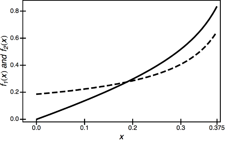
Figure 1: Comparison of the functions $f_{1}(x)$ (dashed line) and $f_{2}(x)$ (solid line) in the range $0<x=\hbar\omega/(\alpha^{2}mc^{2})<3/8$. The overlap occurs at $x=\tfrac{3}{16}$, which is the two-photon resonance condition.

In view of advances in handling the Schrödinger–Coulomb propagator Swainson and Drake (1991a, b, c), and the calculation of energy-dependent matrix elements of the nonrelativistic propagator, which are necessary for analytic Lamb shift calculations Pachucki (1993); Jentschura and Pachucki (1996); Jentschura et al. (1997), it is feasible to write analytic expressions for the two-photon transition matrix element in the velocity and length gauges. We may define the dimensionless matrix element

$$\mathcal{Q}_{2S;1S}(\omega)= \;\frac{(\alpha mc)^{4}}{3m\hbar^{2}}\,Q_{2S;1S}(\omega)$$ (37)

$$= \;\frac{(\alpha mc)^{4}}{3m\hbar^{2}}\,\left<2S\left|\vec{r}\,\frac{1}{H_{A}-E_{n}-\omega}\,\,\vec{r}\right|1S\right>\,,$$

for which we may write the expression

$$\mathcal{Q}_{2S;1S}(\omega)=\frac{512\,\sqrt{2}\,t^{2}}{729\,(t-2)^{3}\,(t^{2}-1)^{2}\,(t+2)^{2}}\,\\[8.61108pt] \times\left(419t^{7}+134t^{6}-15t^{5}+30t^{4}\right.\\ \left.+60t^{3}-120t^{2}-32t+64\right)\\[8.61108pt] -\frac{4096\,\sqrt{2}\;\;{}_{2}F_{1}\left(1,-t,1-t,\frac{(1-t)\,(2-t)}{(1+t)\,(2+t)}\right)}{3\,(t^{2}-2)^{3}\,(t^{2}-1)^{2}}\,$$ (38)

where

$$t=\sqrt{1-\frac{2\,\hbar\omega}{\alpha^{2}mc^{2}}}\,.$$ (39)

(All formulas pertain to atomic hydrogen, where we set the nuclear charge number equal to $Z=1$). The dimensionless matrix element in the velocity gauge is

$$\mathcal{P}_{2S;1S}(\omega)= \;\frac{m}{3\hbar^{2}}\,P_{2S;1S}(\omega)$$ (40)

$$= \;\frac{1}{3m}\,\left<2S\left|\vec{p}\,\frac{1}{H_{A}-E_{n}-\omega}\,\vec{p}\right|1S\right>\,,$$

for which the expression reads

$$\mathcal{P}_{2S;1S}(\omega)=\frac{64\,\sqrt{2}}{81}\,\frac{t^{2}(23\,t^{3}+8\,t^{2}+t-2)}{(t-2)^{2}\,(t^{2}-1)\,(t+2)}\\[8.61108pt] -\frac{256\,\sqrt{2}\;\;{}_{2}F_{1}\left(1,-t,1-t,\frac{(1-t)\,(2-t)}{(1+t)\,(2+t)}\right)}{3\,(t-2)^{2}\,(t^{2}-1)\,(t+2)^{2}}\,.$$ (41)

In Fig. 1, we compare the expressions

$$f_{1}= \;\mathcal{P}_{2S;1S}(\omega)\,,$$ (42a)

$$f_{2}= \;\frac{(E_{2S}-E_{1S}-\hbar\omega)\,(-\hbar\omega)}{(\alpha^{2}\,m\,c^{2})^{2}}\,\mathcal{Q}_{2S;1S}(\omega)$$ (42b)

in the range $\omega\in(0,E_{2S}-E_{1S})$, as a function of $x=\hbar\omega/(\alpha^{2}mc^{2})$. The difference of the results given in Eqs. (41) and (38),

$$\Delta= \;f_{1}-f_{2}$$

$$= \;\frac{m}{\hbar^{2}}\left(\hbar\omega-\tfrac{1}{2}(E_{2S}-E_{1S})\right)\left<2S\left|\vec{r}^{\,2}\right|1S\right>$$

$$= \;-\frac{512\,\sqrt{2}}{729}\left(x-\frac{3}{16}\right)\,,$$ (43)

is plotted in Fig. 2. At exact resonance, one has

$$x=x_{R}=\frac{3}{16}\,,\qquad\Delta=0\,,$$ (44)

as well as

$$\mathcal{Q}_{2S;1S}(\omega_{R})=-\left(\frac{16}{3}\right)^{2}\mathcal{Q}_{2S;1S}(\omega_{R})\\ =-\frac{2^{15}}{3^{6}}\,\left[19\,\sqrt{2}+16\,\sqrt{5}+64\,\sqrt{2}\;\right.\\ \left.\times\phi\left(-19+6\,\sqrt{10},1,-2\,\sqrt{\frac{2}{5}}\right)\right]=-7.853\,655\,422\,.$$ (45)

Here,

$$\phi(z,s,a)=\sum_{k=0}^{\infty}\frac{z^{k}}{(k+a)^{s}}$$ (46)

is the Lerch $\phi$ transcendent.

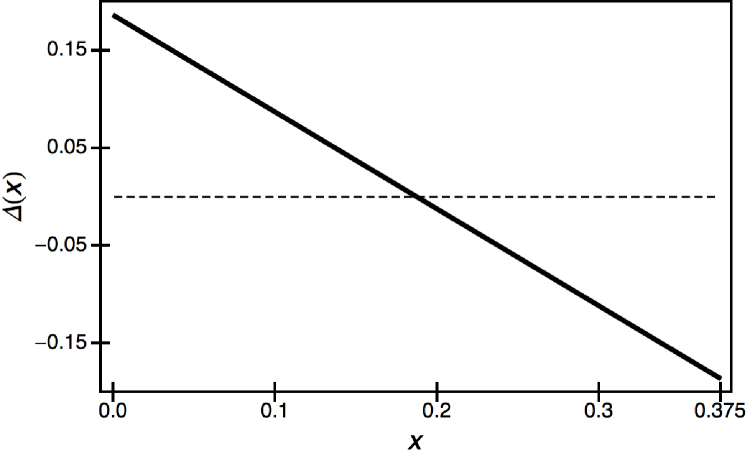
Figure 2: Gauge difference $\Delta(x)=f_{1}(x)-f_{2}(x)$. The zero occurs at $x=\tfrac{3}{16}$.

With Lamb Lamb (1952) and Kobe Kobe (1978), we note that the electric field is a gauge-independent quantity, use the length-gauge expression and supply the prefactors in SI units in order to write the following expression for the Rabi frequency Haas et al. (2006a),

$$\Omega= \;2(2\pi\beta_{2S;1S})\,I_{L}\,,$$ (47)

$$\qquad\beta_{2S;1S}(\omega)= \;-\frac{e^{2}\hbar}{\alpha^{4}m^{3}c^{5}(4\pi\epsilon_{0})}\,\mathcal{Q}_{2S;1S}(\omega)\,.$$ (48)

An expansion of the Rabi frequency about resonance leads to the result

$$\beta_{2S;1S}(\omega)= \;\beta_{2S;1S}(\omega_{R})+\left.\frac{\partial\beta_{2S;1S}(\omega)}{\partial\omega}\right|_{\omega=\omega_{R}}(\omega-\omega_{R})$$ (49)

$$= \;\left[3.68111\times 10^{-5}+2.32293\times 10^{-4}(x-x_{R})\right]\,$$

$$\;\times\frac{{\rm Hz}\,{\rm m}^{2}}{{\rm W}^{2}}\,,$$ (50)

where $x=\omega/(\alpha^{2}m)$ and $x_{R}=3/16$.

A remark on two-color absorption is in order. If an atom is simultaneously subjected to two laser fields of different frequencies $\omega_{1}$ and $\omega$, which fulfill the resonance condition $\omega_{1}+\omega_{2}=E_{f}-E_{i}$, then gauge invariance is restored. On the basis of Eq. (III), this is verified (again for two-photon resonance) as follows,

$$P(\omega_{1})+P(\omega_{2})=(E_{f}-E_{i}-\hbar\omega_{1})(-\hbar\omega_{1})\,Q(\omega_{1})\\ (E_{f}-E_{i}-\hbar\omega_{2})(-\hbar\omega_{2})\,Q(\omega_{2})\\ +\left[\hbar\omega_{1}-\tfrac{1}{2}(E_{f}-E_{i})\right]\,\left<\phi_{f}\left|\vec{r}^{\,2}\right|\phi_{i}\right>\\ +\left[\hbar\omega_{2}-\tfrac{1}{2}(E_{f}-E_{i})\right]\,\left<\phi_{f}\left|\vec{r}^{\,2}\right|\phi_{i}\right>\\ =-(\hbar\omega_{1})(\hbar\omega_{2})\,[Q(\omega_{1})+Q(\omega_{2})]\,.$$ (51)

The relation $P(\omega_{1})+P(\omega_{2})=-(\hbar\omega_{1})(\hbar\omega_{2})\,[Q(\omega_{1})+Q(\omega_{2})]$ is equivalent to the gauge invariance of the resonant two-color, two-photon transition. In Tables I and II of Ref. Bassani et al. (1977), the authors present resonant two-color, two-photon matrix elements which in our notation would read

$$\mathcal{Q}_{\rm 2c;2\gamma}(\omega_{1})=\frac{3}{4}\,\left[\mathcal{Q}_{2S;1S}(\omega_{1})+\mathcal{Q}_{2S;1S}(\omega_{2})\right]\,,$$ (52)

where, again, $\omega_{2}=E_{f}-E_{i}-\omega_{1}$. For example, the gauge-invariant resonant two-color result at frequency $\frac{28}{15}\omega_{R}$ reads as

$$\mathcal{Q}_{2c;2\gamma}\left(\omega_{1}=\frac{28}{15}\omega_{R}=\frac{7}{20}\frac{\alpha^{2}mc^{2}}{\hbar}\right)=-\frac{160\,000}{343}\\ \times\Biggl{[}157\sqrt{2}+56\sqrt{15}+2\sqrt{190}\\ +560\,\sqrt{2}\;\phi\left(\tfrac{1}{7}\,(-263+48\,\sqrt{30}),1,-\sqrt{\frac{10}{3}}\right)\\ +64\,\sqrt{2}\;\phi\left(\tfrac{1}{7}\,(-848+87\,\sqrt{95}),1,-2\sqrt{\frac{5}{19}}\right)\Biggr{]}\\ =-62.659\,473\,633\,,$$ (53)

verifying the fifth entry in the last row of Tables I and II of Ref. Bassani et al. (1977). Diagrammatically, the two terms in Eq. (52) correspond to photon absorption processes with two different possible time orderings of the absorptions of photons with frequencies $\omega_{1}$ and $\omega_{2}$.

V Conclusions

In the current paper, we (re-)examine the transformation from the length to the velocity gauge in Sec. II, and recall that the length-gauge and velocity-gauge Hamiltonians are not related by a unitary transformation. Furthermore, we show that the physical interpretation of a quantum mechanical operator depends on the gauge, vindicating arguments given by Lamb Lamb (1952) and Kobe Kobe (1978) regarding the applicability of the length gauge off resonance. In Sec. III, we consider the ac Stark shift as a paradigmatic example of a physical process invariant under an “extended” gauge transformation. Specifically, in atomic hydrogen, we rederive the known result Haas et al. (2006b, a) that the ac Stark shift formulated in the length gauge is equal to the velocity-gauge expression, even if the gauge transformation of the wave function is ignored. The derivation is based on the “master identity” given in Eq. (III). In Sec. IV, we investigate the two-photon transition matrix element, where the “extended gauge invariance” does not hold off resonance. The derivation again profits from the general identity (III), which can be applied to both of the problems studied in Secs. III and IV; its validity is verified on the basis of analytic and numerical calculations [see Eqs. (38), (41) as well as Figs. 1 and 2]. In retrospect, it would have seemed somewhat surprising if extended gauge invariance had been applicable to two-photon transitions (under the inclusion of all possible virtual, intermediate states) but failed for one-photon transitions [see Eqs. (II)—(II)]. We conclude that for two-photon transitions, the length gauge needs to be used off resonance, just as for one-photon absorption.

Yet, for two-color, two-photon absorption with the sum of the two photon frequencies adding up to the exact resonance frequency, extended gauge invariance again holds (see Sec. IV and Ref. Bassani et al. (1977)).

A few explanatory remarks are in order. We have seen that extended gauge invariance is restored at exact resonance, for both one- as well as (one-color and two-color) two-photon transitions. Mathematically, extended gauge invariance is restored at resonance in view of commutation relations, notably, $\vec{p}=\frac{{\mathrm{i}}m}{\hbar}[H_{A},\vec{r}]$, where $H_{A}$ is the atomic Schrödinger–Coulomb Hamiltonian. Physically, extended gauge invariance holds because processes at exact resonance, or, processes which involve energy shifts, can be formulated using a form of the interaction where the fields and potentials are adiabatically switched off in the infinite future and in the infinite past, using a damping term of the form $\exp(-\epsilon|t|)$. The gauge transformation of the wave functions (in and out states) then proceeds in the distant past and future, where the fields are switched off and the gauge transformation is just the identity. For one- and two-photon transitions, the necessity to introduce the damping terms is inherent to the formulation of Fermi’s Golden Rule, which describes transition rates at exact resonance, where the initial and final states fulfill an energy conservation condition [see Refs. Sakurai (1994, 1967).

The ac Stark shift can be formulated using the Gell–Mann–Low theorem [see Eqs. (19) and (21) of Ref. Haas et al. (2006b)], in which case one uses a time evolution operator that evolves the wave function from the infinite past to the present, with the interactions being switched off for $t\to-\infty$. Within the Gell–Mann–Low formalism, the gauge transformation of the wave function in the infinite past amounts to the identity transformation, because the interactions are adiabatically switched off in this limit. The extended gauge invariance of those physical processes whose description allows such an adiabatic damping, thus finds a natural explanation. For one- and two-photon transitions off resonance, however, the quantum dynamics are instantaneous, and the physical interpretation of the operators must be carefully restored. In this case, only the length gauge provides a consistent physical description (see the discussion in Sec. II).

One might thus ask if the velocity gauge has any advantages in the physical description of laser-related processes. The answer can be given as follows. There are $S$-matrix elements in the so-called strong-field approximation whose evaluation becomes easier in the velocity gauge. In this case, the in- and out-states are asymptotic states [the $S$ matrix is a time evolution operator from the infinite past to the infinite future]. Indeed, as stressed by Reiss in Eqs. (29) and (31) of Ref. Reiss , the Volkov state in a strong laser field is much easier to formulate in the velocity gauge, and consequently, $S$-matrix calculations should preferentially be done in this gauge [see also Refs. Reiss (1992); Cormier and Lambropoulos (1996); Reiss ]. In the formulation of the $S$ matrix, one canonically uses infinitesimal damping parameters [see Ref. Mohr et al. (1998)], and thus, extended gauge invariance is restored. We conclude that the choice of gauge in these cases should be made according to practical considerations, and in strong laser fields, the velocity gauge provides for the most simple computational framework.

References

- Lamb (1952) W. E. Lamb, “Fine Structure of the Hydrogen Atom. III,” Phys. Rev. 85, 259–276 (1952).
- Bassani et al. (1977) F. Bassani, J. J. Forney, and A. Quattropani, “Choice of gauge in two-photon transitions: 1s-2s transition in atomic hydrogen,” Phys. Rev. Lett. 39, 1070–1073 (1977).
- Kobe (1978) D. H. Kobe, “Question of Gauge: Nonresonant Two-Photon Absorption,” Phys. Rev. Lett. 40, 538 (1978).
- Schlicher et al. (1984) R. R. Schlicher, W. Becker, J. Bergou, and M. O. Scully, “Interaction hamiltonian in quantum optics or: vs. revisited,” in Quantum Electrodynamics and Quantum Optics, edited by A.-O. Barut (Phys. Lett., New York, 1984) pp. 405–441.
- Power and Thirunamachandran (1975) E. A. Power and T. Thirunamachandran, “On the matrix element for two-photon absorption,” J. Phys. B 5, L170–L172 (1975).
- Power and Thirunamachandran (1978) E. A. Power and T. Thirunamachandran, “On the nature of the Hamiltonian for the interaction of radiation with atoms and molecules: , , and all that,” Am. J. Phys. 46, 370–378 (1978).
- Jentschura and Noble (2013) U. D. Jentschura and J. H. Noble, “Nonrelativistic Limit of the Dirac–Schwarzschild Hamiltonian: Gravitational Zitterbewegung and Gravitational Spin–Orbit Coupling,” Phys. Rev. A 88, 022121 (2013).
- (8) H. R. Reiss, Limitations of gauge invariance, e-print arXiv:1302.1212 [quant-ph].
- Jentschura et al. (2003) U. D. Jentschura, J. Evers, M. Haas, and C. H. Keitel, “Lamb Shift of Laser-Dressed Atomic States,” Phys. Rev. Lett. 91, 253601 (2003).
- Jentschura and Keitel (2004) U. D. Jentschura and C. H. Keitel, “Radiative corrections in laser–dressed atoms: Formalism and applications,” Ann. Phys. (N.Y.) 310, 1–55 (2004).
- Evers et al. (2004) J. Evers, U. D. Jentschura, and C. H. Keitel, “Relativistic and Radiative Corrections to the Mollow Spectrum,” Phys. Rev. A 70, 062111 (2004).
- Jentschura et al. (2005) U. D. Jentschura, J. Evers, and C. H. Keitel, “Relativistic and radiative corrections to multi–level mollow–type spectra,” Laser Phys. 15, 37–45 (2005).
- Craig and Thirunamachandran (1984) D. P. Craig and T. Thirunamachandran, Molecular Quantum Electrodynamics (Dover Publications, Mineola, NY, 1984).
- Jentschura and Pachucki (2015) U. D. Jentschura and K. Pachucki, “Functional Form of the Imaginary Part of the Atomic Polarizability,” Eur. Phys. J. D 69, 118 (2015).
- Geltman (1963) S. Geltman, “Double–Photon Photo–Detachment of Negative Ions,” Phys. Lett. 4, 168–169 (1963).
- Swainson and Drake (1991a) R. A. Swainson and G. W. F. Drake, “A unified treatment of the non-relativistic and relativistic hydrogen atom I: the wavefunctions,” J. Phys. A 24, 79–94 (1991a).
- Swainson and Drake (1991b) R. A. Swainson and G. W. F. Drake, “A unified treatment of the non-relativistic and relativistic hydrogen atom II: the Green functions,” J. Phys. A 24, 95–120 (1991b).
- Swainson and Drake (1991c) R. A. Swainson and G. W. F. Drake, “A unified treatment of the non-relativistic and relativistic hydrogen atom III: the reduced Green functions,” J. Phys. A 24, 1801–1824 (1991c).
- Pachucki (1993) K. Pachucki, “Higher-Order Binding Corrections to the Lamb Shift,” Ann. Phys. (N.Y.) 226, 1–87 (1993).
- Jentschura and Pachucki (1996) U. Jentschura and K. Pachucki, “Higher-order binding corrections to the Lamb shift of states,” Phys. Rev. A 54, 1853–1861 (1996).
- Jentschura et al. (1997) U. D. Jentschura, G. Soff, and P. J. Mohr, “Lamb shift of 3P and 4P states and the determination of ,” Phys. Rev. A 56, 1739–1755 (1997).
- Haas et al. (2006a) M. Haas, U. D. Jentschura, C. H. Keitel, N. Kolachevsky, M. Herrmann, P. Fendel, M. Fischer, Thomas Udem, R. Holzwarth, T. W. Hänsch, M. O. Scully, and G. S. Agarwal, “Two-photon excitation dynamics in bound two-body coulomb systems including ac stark shift and ionization,” Phys. Rev. A 73, 052501 (2006a).
- Haas et al. (2006b) M. Haas, U. D. Jentschura, and C. H. Keitel, “Classical vs. Second–Quantized Description of the Dynamic Stark Shift,” Am. J. Phys. 74, 77–81 (2006b).
- Sakurai (1994) J. J. Sakurai, Modern Quantum Mechanics (Addison-Wesley, Reading, MA, 1994).
- Sakurai (1967) J. J. Sakurai, Advanced Quantum Mechanics (Addison-Wesley, Reading, MA, 1967).
- Reiss (1992) H. R. Reiss, “Theoretical Methods in Quantum Optics: S–Matrix and Keldysh Techniques for Strong–Field Processes,” Prog. Quant. Electr. 16, 1–71 (1992).
- Cormier and Lambropoulos (1996) E. Cormier and P. Lambropoulos, “Optimal gauge and gauge invariance in non-perturbative time-dependent calculation of above-threshold ionization,” J. Phys. B 29, 1667–1680 (1996).
- Mohr et al. (1998) P. J. Mohr, G. Plunien, and G. Soff, “QED corrections in heavy atoms,” Phys. Rep. 293, 227–372 (1998).