Theory of noncontact friction for atom-surface interactions

Abstract

The noncontact (van der Waals) friction is an interesting physical effect which has been the subject of controversial scientific discussion. The “direct” friction term due to the thermal fluctuations of the electromagnetic field leads to a friction force proportional to $1/{\mathcal{Z}}^{5}$ (where ${\mathcal{Z}}$ is the atom-wall distance). The “backaction” friction term takes into account the feedback of thermal fluctuations of the atomic dipole moment onto the motion of the atom and scales as $1/{\mathcal{Z}}^{8}$. We investigate noncontact friction effects for the interactions of hydrogen, ground-state helium and metastable helium atoms with $\alpha$-quartz (SiO₂), gold (Au) and calcium difluorite (CaF₂). We find that the backaction term dominates over the direct term induced by the thermal electromagnetic fluctuations inside the material, over wide distance ranges. The friction coefficients obtained for gold are smaller than those for SiO₂ and CaF₂ by several orders of magnitude.

I Introduction

Noncontact friction arises in atom-surface interactions; the theoretical treatment has given rise to some discussion Levitov (1989); Polevoi (1990); Høye and Brevik (1992); *HoBr1993; Mkrtchian (1995); Tomassone and Widom (1997); Persson and Zhang (1998); *DeKy1999; *DeKy2001; *DeKy2002; Dedkov and Kyasov (2002b); Volokitin and Persson (1999); *VoPe2001prb; Volokitin and Persson (2002, 2003); *VoPe2005; *VoPe2006; *VoPe2007; *VoPe2008; Dorofeyev et al. (2001). In a simplified understanding, for an ion flying by a dielectric surface (“wall”), the quantum friction effect can be understood in terms of Ohmic heating of the material by the motion of the image charge inside the medium. Alternatively, one can understand it in terms of the thermal fluctuations of the electric fields in the vicinity of the dielectric, and the backreaction onto the motion of the ion or atom in the vicinity of the “wall”.

It has recently been argued that one cannot separate the van-der-Waals force, at finite temperature, from the friction effect Volokitin and Persson (2002). The backaction effect is due to the fluctuations of the atomic dipole moment Volokitin and Persson (2002), which are mirrored by the wall and react back onto the atom; this leads to an additional contribution to the friction force. In contrast to the “direct” term created by the electromagnetic field fluctuations inside the medium Tomassone and Widom (1997) (proportional to $1/{\mathcal{Z}}^{5}$ where ${\mathcal{Z}}$ is the atom-wall distance), the backaction term leads to a $1/{\mathcal{Z}}^{8}$ effect. A comparison of the magnitude of these two effects, for realistic dielectric response functions of materials, and using a detailed model of the atomic polarizability, is the subject of the current paper. While the $1/{\mathcal{Z}}^{8}$ effect is parametrically suppressed for large atom-wall separations, the numerical coefficients may still change the hierarchy of the effects.

We should also note that the direct term Tomassone and Widom (1997); Volokitin and Persson (2002) can be formulated as an integral over the imaginary part of the polarizability, and of the dielectric response function of the material. Recently, we found a conceptually interesting “one-loop” dominance for the imaginary part of the polarizability Jentschura et al. (2015); Jentschura and Pachucki (2015). The imaginary part of the polarizability describes a process where the atom emits radiation at the same frequency as the incident laser radiation, but in a different direction. Note that, by contrast, Rabi flopping involves continuous absorption and emission into the laser mode; the laser-dressed states Scully and Zubairy (1997); Jentschura and Keitel (2004) are superpositions of states $|g,n_{L}+1\rangle$ and $|e,n_{L}\rangle$, where $n_{L}$ is the number of laser photons while $|g\rangle$ and $|e\rangle$ denote the atomic ground and excited states. A priori, this Rabi flopping may proceed off resonance.

Figure 1: Feynman diagrams contributing to the imaginary part of the polarizability. A photon is absorbed from a bath (denoted by the external crosses), while a second photon of equal frequency (nonresonant with respect to an atomic transition) is emitted (Cutkosky rules).

By contrast, when the ac Stark shift of an atomic level is formulated perturbatively and the second-order shift of the atomic level in the external laser field is evaluated using a second-quantized formalism (see Sec. III of Ref. Haas et al. (2006)), a resonance condition has to be fulfilled in order for an imaginary part of the energy shift to be generated. Namely, the final state of atom$+$field in the decay process has to have exactly the same energy as the reference state of atom$+$field. This is possible only at exact resonance, when the emitted photon has just the right frequency to compensate the “quantum jump” of the bound electron from an excited state to an energetically lower state Sakurai (1994, 1967); Haas et al. (2006). The ac Stark shift is proportional to the atomic polarizability. Its tree-level imaginary part Jentschura et al. (2015); Jentschura and Pachucki (2015) corresponds to spontaneous emission of the atom at an exact resonance frequency, still, not necessarily along the same direction as the incident laser photon. When quantum electrodynamics is involved, it is seen that due to quantum fluctuations of the electromagnetic field, spontaneous emission is possible off resonance. In Refs. Jentschura et al. (2015); Jentschura and Pachucki (2015), the imaginary part of the polarizability was found to be dominated by a self-energy correction to the ac Stark shift. Physically, the imaginary part of the polarizability corresponds to a “decay rate” of the reference state $|\phi,n_{L}\rangle$ used in the calculation of the ac Stark shift, to a state $|\phi,n_{L}-1,1_{\vec{k}\lambda}\rangle$, where $|\phi\rangle$ is the atomic reference state, the occupation number of the laser mode is $n_{L}$, and there is either zero or one photon in the mode $\vec{k}\lambda$. While the laser frequency is equal to the frequency of the emitted radiation ($\omega_{L}=\omega_{\vec{k}}$), the emission proceeds into a different direction as compared to the laser wave vector ($\vec{k}\neq\vec{k}_{L}$). Off resonance, the quantum electrodynamic one-loop effect calculated in Refs. Jentschura et al. (2015); Jentschura and Pachucki (2015) thus dominates the imaginary part of the polarizability, not the tree-level term. This is quite surprising; the relevant Feynman diagrams are shown in Fig. 1. The peculiar behavior of the imaginary part of the polarizability suggests a detailed numerical study of the noncontact friction integral Tomassone and Widom (1997); Volokitin and Persson (2002), and comparison, of the direct and backaction terms.

This paper is organized as follows. In Sec. II, we attempt to shed some light on the derivation of the effect. Full SI mksA units are kept throughout the derivation. The numerical calculations of noncontact friction for the hydrogen and helium interactions with $\alpha$-quartz, gold, and CaF₂ are described in Sec. III, where we shall use atomic units for for frequency data and friction coefficients in Tables 1—5. We employ a convenient fit to the vibrational and interband excitations of the $\alpha$-quartz and CaF₂ lattices. Finally, conclusions are drawn in Sec. IV.

II Derivation

Our derivation is in part inspired by Ref. Volokitin and Persson (2002); we supplement the discussion with some explanatory remarks and simplified formulas where appropriate. The electric field at the position of the atomic dipole (i.e., at the position of the atom) is written as

$$\vec{E}(t)=\vec{E}_{0}\,{\mathrm{e}}^{-{\mathrm{i}}\,\omega\,t}+\vec{E}_{1}\,{\mathrm{e}}^{-{\mathrm{i}}\,(\omega+\omega_{0})\,t}\,,$$ (1)

where $\omega$ is the angular frequency component of the (thermal) fluctuation, and $\omega_{0}$ describes a small displacement of the atom’s position itself. The contribution proportional to $\vec{E}_{1}$ is included as a result of a backaction term, which takes the variation of the spontaneous and induced fields over the spatial amplitude of the oscillatory motion of the atom into account [see Eq. (II)]. Hence, the angular frequency of the motion ($\omega_{0}$) is added to the thermal frequency, and the term is proportional to $\exp[-{\mathrm{i}}(\omega+\omega_{0})\,t]$. The displacement of the atom is of angular frequency $\omega_{0}$,

$$\vec{u}(t)=\vec{u}_{0}\,{\mathrm{e}}^{-{\mathrm{i}}\omega_{0}t}\,,\qquad\vec{r}(t)=\vec{r}_{0}+\vec{u}(t)\,.$$ (2)

The dipole density of the isolated atom is supposed to perform oscillations of the form

$$\vec{d}(\vec{r},t)= \;\vec{d}_{0}\,\delta^{(3)}(\vec{r}-\vec{r}_{0})\,{\mathrm{e}}^{-{\mathrm{i}}\omega t}+\vec{p}_{1}(\vec{r},\omega)\,{\mathrm{e}}^{-{\mathrm{i}}(\omega+\omega_{0})\,t}\,,$$

$$\vec{p}_{1}(\vec{r},\omega)= \;\vec{d}_{1}\,\delta^{(3)}(\vec{r}-\vec{r}_{0})-\vec{d}_{0}\,\vec{u}_{0}\cdot\vec{\nabla}\delta^{(3)}(\vec{r}-\vec{r}_{0})\,.$$ (3)

Here, the second term is generated by the displacement of the atom, i.e., by the expansion of the Dirac $\delta$ function $\delta^{(3)}(\vec{r}-\vec{r}_{0}-\vec{u}(t))$ to first order in $\vec{u}(t)$. While the atomic dipole moment is a sum of a fluctuating term $\vec{d}^{f}$ and an induced term (by the corresponding frequency component of the electric field at the position of the atom),

$$d_{0i}=d^{f}_{i}+\alpha(\omega)\,E_{0i}\,,$$ (4)

the frequency component for $\omega+\omega_{0}$ only contains an induced term, $\vec{d}_{1}=\alpha(\omega+\omega_{0})\,\vec{E}_{1}$.

Let $G_{ij}(\vec{r},\vec{r}_{0},\omega)$ denote the frequency component of the Green tensor which determines the electric field generated at position $\vec{r}$ by a point dipole at $\vec{r}_{0}$. In the nonretardation approximation [Eq. (1) of Ref. Tomassone and Widom (1997)], it reads

$$g(\vec{r},\vec{r}^{\prime},\omega)= \;\frac{1}{4\pi\epsilon_{0}}\,\left(\frac{1}{|\vec{r}-\vec{r}^{\prime}|}\right.$$

$$\;\left.-\frac{\epsilon(\omega)-1}{\epsilon(\omega)+1}\,\frac{1}{|\vec{r}-\vec{r}^{\prime}+2\hat{n}_{\perp}(\vec{r}^{\prime}\cdot\hat{n}_{\perp})|}\right)\,,$$

$$G_{ij}(\vec{r},\vec{r}^{\prime},\omega)= \;-\nabla_{i}\nabla^{\prime}_{j}\,g(\vec{r},\vec{r}^{\prime},\omega)\,.$$ (5)

Here, $\hat{n}=\hat{e}_{z}$ is the surface normal (the surface of the dielectric is the $xy$ plane). The result

$$G_{zz}(\vec{0},\vec{r}_{\mathcal{Z}},\omega)=\frac{2}{{\mathcal{Z}}^{3}}+\frac{\epsilon(\omega)-1}{\epsilon(\omega)+1}\frac{2}{{\mathcal{Z}}^{3}}\,,\quad\vec{r}_{\mathcal{Z}}=\hat{e}_{z}\,{\mathcal{Z}}\,,$$ (6)

reflects the fact that a dipole oriented in parallel to the $z$ axis generates a mirror dipole which also is oriented in parallel to the $z$ axis (not antiparallel, see the dipoles in Fig. 2). Because of this, the second term on the right-hand side of Eq. (6) has the same sign as the first term.

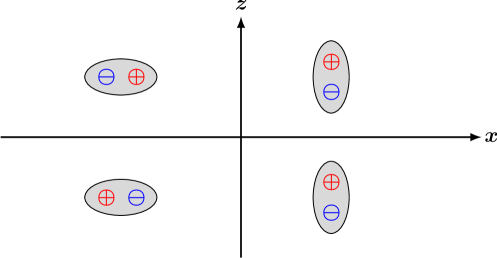
Figure 2: (Color online.) Mirroring a dipole in the $xy$ plane. A dipole aligned along the $x$ axis gives rise to an antiparallel mirror dipole, whereas a dipole aligned along the $z$ axis gives rise to a parallel mirror dipole. Recall that mirror charges have the opposite sign as compared to the original ones.

Self-consistency dictates that the field $\vec{E}_{0}\equiv\vec{E}_{0}(\vec{r}_{0})$ at the position of the atom is equal to the sum of the field generated by the dipole moment $d_{0i}$, and the fluctuating component $E^{s}_{i}(\vec{r}_{0},\omega)$ of the electric field,

$$E_{0i}= \;G_{ii}(\vec{r}_{0},\vec{r}_{0},\omega)\,d_{0i}+E^{s}_{i}(\vec{r}_{0},\omega)$$

$$= \;G_{ii}(\vec{r}_{0},\vec{r}_{0},\omega)\,\alpha(\omega)E_{0i}+G_{ii}(\vec{r}_{0},\vec{r}_{0},\omega)\,d^{f}_{i}$$

$$\;+E^{s}_{i}(\vec{r}_{0},\omega)\,,$$ (7)

where no summation over $i$ is carried out (one has $G_{ij}=G_{ii}\,\delta_{ij}$ at equal spatial coordinates). So,

$$E_{0i}= \;\frac{G_{ii}(\vec{r}_{0},\vec{r}_{0},\omega)\,d^{f}_{i}+E^{s}_{i}(\vec{r}_{0},\omega)}{1-G_{ii}(\vec{r}_{0},\vec{r}_{0},\omega)\,\alpha(\omega)}\,,$$ (8a)

$$d_{0i}= \;\frac{d^{f}_{i}+\alpha(\omega)\,E^{s}_{i}(\vec{r}_{0},\omega)}{1-\alpha(\omega)\,G_{ii}(\vec{r}_{0},\vec{r}_{0},\omega)}\,,$$ (8b)

where in Eq. (8b) we have taken into account Eq. (4). The electric field $\vec{E}_{0}$ and the dipole moment $\vec{d}_{0}$ are given in terms of fluctuating terms; the denominators in Eq. (8) take the backaction into account. For $\vec{E}_{1}$, one observes that the gradient term in the expression of $\vec{p}_{1}(\vec{r},\omega)$ [Eq. (II)], in the non-fluctuating contribution $\int{\mathrm{d}}^{3}r^{\prime}\,G_{ij}(\vec{r},\vec{r}^{\prime},\omega+\omega_{0})\,p_{1j}(\vec{r},\omega)$, needs to be treated by partial integration. Adding the term due to the fluctuations of the atom’s position, and due to the spontaneous fluctations of the electromagnetic field, one obtains

$$E_{1i}= \;G_{ii}(\vec{r}_{0},\vec{r}_{0},\omega+\omega_{0})\,\alpha(\omega+\omega_{0})\,E_{1i}$$

$$\;+\vec{u}_{0}\cdot\vec{\nabla}_{\vec{r}}\left(E^{s}_{i}(\vec{r},\omega)+G_{ij}(\vec{r}_{0},\vec{r},\omega+\omega_{0})\,d_{0j}\right.$$

$$\;\left.\left.+G_{ij}(\vec{r},\vec{r}_{0},\omega)\,d_{0j}\right)\right|_{\vec{r}=\vec{r}_{0}}\,.$$ (9)

This equation can be trivially solved for $\vec{E}_{1}$. The thermal fluctuations are described by the following equations Tomassone and Widom (1997),

$$\left<d^{f}_{i}\,d^{f}_{j}\right>_{\omega}= \;\frac{2\,\Theta(\omega,T)}{\omega}\,\delta_{ij}\,{\rm Im}\,\alpha(\omega)\,,$$ (10a)

$$\left<E_{i}(\vec{r})\,E_{j}(\vec{r}^{\prime})\right>_{\omega}= \;\frac{2\,\Theta(\omega,T)}{\omega}\,{\rm Im}[G_{ij}(\vec{r},\vec{r}^{\prime},\omega)]\,.$$ (10b)

where $\Theta(\omega,T)=\hbar\,\omega\,\left({\textstyle{\frac{1}{2}}}+n(\omega)\right)={\textstyle{\frac{1}{2}}}\hbar\,\omega\,\coth\left({\textstyle{\frac{1}{2}}}\,\beta\,\hbar\,\omega\right)$ is the Kallen–Welton thermal factor, with $n(\omega)=[\exp(\beta\,\hbar\,\omega)-1]^{-1}$, and $\beta=1/(k_{B}\,T)$ where $k_{B}$ is the Boltzmann constant. With the help of $\rho=-\vec{\nabla}\cdot\vec{p}$ and $\vec{j}=\partial_{t}\vec{p}$, one formulates a time-dependent force,

$$\vec{F}(t)= \;\int{\mathrm{d}}^{3}r\,\left<\rho(\vec{r},t)\,\vec{E}^{*}(\vec{r},t)+\vec{j}(\vec{r},t)\times\vec{B}^{*}(\vec{r},t)\right>$$

$$= \;\vec{F}_{s}(t)+\vec{u}_{0}\cdot\frac{\partial}{\partial r}\vec{F}_{s}(t)+\vec{F}_{f}(\omega,\omega_{0})\,{\mathrm{e}}^{-{\mathrm{i}}\omega_{0}\,t}\,.$$ (11)

Here, $F_{s}(t)$ is the static van-der-Waals force, $\vec{u}_{0}\cdot\frac{\partial}{\partial r}\vec{F}_{s}(t)$ describes the variation of the van-der-Waals force with the oscillating position of the atom, and $\vec{F}_{f}(\omega,\omega_{0})$ is a Fourier component of the friction force. An integration over the thermal fluctuations of all Fourier components of the friction force gives the total friction force,

$$\vec{F}_{f}= \;\frac{1}{2}\,\left.\int_{0}^{\infty}\frac{{\mathrm{d}}\omega}{2\pi}\;\omega_{0}\,\frac{\partial}{\partial\omega_{0}}\left<\vec{F}(\omega,\omega_{0})\right>\right|_{\omega_{0}=0}$$

$$= \;{\mathrm{i}}\,\omega_{0}\,\left[\eta_{x}\,(u_{0x}\hat{e}_{x}+u_{0y}\hat{e}_{y})+\eta_{z}\,u_{z}\hat{e}_{z}\right]$$

$$= \;-\eta_{x}\,(v_{x}\hat{e}_{x}+v_{y}\hat{e}_{y})-\eta_{z}v_{z}\hat{e}_{z}\,.$$ (12)

Here, $\eta_{x}$ and $\eta_{z}$ are the friction coefficient for motion along the $x$ and $z$ directions, respectively. The additional assumption of a small mechanical motion with velocity $\vec{v}=\partial_{t}\left.\vec{u}_{0}{\mathrm{e}}^{-{\mathrm{i}}\omega_{0}t}\right|_{t=0}=-{\mathrm{i}}\omega_{0}\,\vec{u}_{0}$ is made.

The result for $\eta_{x}$ is obtained as,

$$\eta_{x}= \;\frac{\beta\hbar^{2}}{2\pi}\,\int_{0}^{\infty}\frac{{\mathrm{d}}\omega}{\sinh^{2}({\textstyle{\frac{1}{2}}}\,\beta\,\hbar\,\omega)}\,\left[\sum_{\ell=x,y,z}\frac{\partial^{2}}{\partial x\,\partial x^{\prime}}\mathrm{Im}G_{\ell\ell}(\vec{r},\vec{r}^{\prime},\omega)\,\mathrm{Im}\left(\frac{\alpha(\omega)}{1-\alpha(\omega)\,G_{\ell\ell}(\vec{r}_{\mathcal{Z}},\vec{r}_{\mathcal{Z}},\omega)}\right)\right.$$

$$\;\left.\left.-2|\alpha(\omega)|^{2}\,\mathrm{Re}\left(\frac{1}{(1-\alpha^{*}(\omega)\,D^{*}_{zz}(\vec{r}_{\mathcal{Z}},\vec{r}_{\mathcal{Z}},\omega))(1-\alpha(\omega)\,G_{zz}(\vec{r}_{\mathcal{Z}},\vec{r}_{\mathcal{Z}},\omega))}\right)\,\left(\frac{\partial}{\partial x}G_{xz}(\vec{r},\vec{r}_{\mathcal{Z}},\omega)\right)^{2}\right]\right|_{\vec{r},\vec{r}^{\prime}=\vec{r}_{\mathcal{Z}}}$$

$$\approx \;\frac{\beta\hbar^{2}}{2\pi}\,\int_{0}^{\infty}\frac{{\mathrm{d}}\omega}{\sinh^{2}({\textstyle{\frac{1}{2}}}\,\beta\,\hbar\,\omega)}\,\left[\sum_{\ell=x,y,z}\frac{\partial^{2}}{\partial x\,\partial x^{\prime}}\mathrm{Im}[G_{\ell\ell}(\vec{r},\vec{r}^{\prime},\omega)]\,\mathrm{Im}[\alpha(\omega)]+\alpha(\omega)^{2}\right.$$

$$\;\left.\left.\times\left\{\sum_{\ell=x,y,z}\left\{\frac{\partial^{2}}{\partial x\,\partial x^{\prime}}\mathrm{Im}[G_{\ell\ell}(\vec{r},\vec{r}^{\prime},\omega)]\,\mathrm{Im}[G_{\ell\ell}(\vec{r}_{\mathcal{Z}},\vec{r}_{\mathcal{Z}},\omega)]\right\}-2\left(\frac{\partial}{\partial x}\mathrm{Im}\left[G_{xz}(\vec{r},\vec{r}_{\mathcal{Z}},\omega)\right]\right)^{2}\right\}\right]\right|_{\vec{r},\vec{r}^{\prime}=\vec{r}_{\mathcal{Z}}}\,.$$ (13)

This result can be written as $\eta_{x}=\eta_{x}^{(1)}+\eta_{x}^{(2)}$, where $\eta_{x}^{(2)}$ is generated by the term in curly brackets in the integrand. With the help of $\sum_{\ell}\frac{\partial^{2}}{\partial x\,\partial x^{\prime}}\mathrm{Im}\,G_{\ell\ell}(\vec{r},\vec{r}^{\prime})=\mathrm{Im}\left(\frac{\epsilon(\omega)-1}{\epsilon(\omega)+1}\right)\,\frac{3}{16\pi\epsilon_{0}\,{\mathcal{Z}}^{5}}$, one verifies that the leading-order, linear term in the polarizability (see Ref. Tomassone and Widom (1997)), from Eq. (II), is given as

$$\eta^{(1)}_{x}= \;\frac{\beta\hbar^{2}}{2\pi}\,\int_{0}^{\infty}\frac{{\mathrm{d}}\omega}{\sinh^{2}({\textstyle{\frac{1}{2}}}\,\beta\,\hbar\,\omega)}\sum_{\ell=x,y,z}\frac{\partial^{2}}{\partial x\,\partial x^{\prime}}\mathrm{Im}G_{\ell\ell}(\vec{r},\vec{r}^{\prime})\,\mathrm{Im}\left(\alpha(\omega)\right)=\frac{3\beta\hbar^{2}}{32\pi^{2}\epsilon_{0}{\mathcal{Z}}^{5}}\,\int_{0}^{\infty}\frac{{\mathrm{d}}\omega\,\mathrm{Im}[\alpha(\omega)]}{\sinh^{2}({\textstyle{\frac{1}{2}}}\,\beta\,\hbar\,\omega)}\mathrm{Im}\left(\frac{\epsilon(\omega)-1}{\epsilon(\omega)+1}\right).$$ (14)

In Eq. (II), the term of second order in the polarizability is given as follows,

$$\eta^{(2)}_{x}= \;\left.\frac{\beta\hbar^{2}}{8\pi}\,\int\limits_{0}^{\infty}\frac{{\mathrm{d}}\omega\,\alpha(\omega)^{2}}{\sinh^{2}({\textstyle{\frac{1}{2}}}\,\beta\,\hbar\,\omega)}\,\left[\left\{\frac{\partial^{2}}{\partial z^{2}}\mathrm{Im}\,G_{zz}(\vec{r},\vec{r}_{\mathcal{Z}},\omega)\right\}\,\mathrm{Im}\,G_{zz}(\vec{r}_{\mathcal{Z}},\vec{r}_{\mathcal{Z}},\omega)-2\,\left(\frac{\partial}{\partial z}\mathrm{Im}\,G_{zz}(\vec{r},\vec{r}_{\mathcal{Z}},\omega)\right)^{2}\right]\right|_{\vec{r},\vec{r}^{\prime}=\vec{r}_{\mathcal{Z}}}$$

$$= \;\frac{9\beta\hbar^{2}}{4096\,\pi^{3}\,\epsilon_{0}^{2}\,{\mathcal{Z}}^{8}}\,\int\limits_{0}^{\infty}{\mathrm{d}}\omega\,\frac{\alpha(\omega)^{2}}{\sinh^{2}({\textstyle{\frac{1}{2}}}\,\beta\,\hbar\,\omega)}\left[\mathrm{Im}\left(\frac{\epsilon(\omega)-1}{\epsilon(\omega)+1}\right)\right]^{2}\,.$$ (15)

For friction in the $z$ direction, one derives $\eta_{z}=\eta_{z}^{(1)}+\eta_{z}^{(2)}$, with $\eta_{z}^{(1)}=2\,\eta^{(2)}_{z}$ and $\eta_{z}^{(2)}=7\,\eta^{(2)}_{x}$, confirming Ref. Volokitin and Persson (2002). The term $\eta^{(2)}$ is generated by the “backaction denominators” from Eqs. (8a) and (8b). For the numerical evaluation of the term $\eta^{(1)}$, the following result

$${\rm Im}[\alpha(\omega)]= \;{\rm Im}[\alpha_{R}(\omega)]+\frac{\omega^{3}}{6\pi\epsilon_{0}c^{3}}\,[\alpha(\omega)]^{2}\,,$$ (16a)

$${\rm Im}\left[\alpha_{R}(\omega)\right]= \;{\rm Im}\left[\alpha_{r}(\omega)\right]-{\rm Im}\left[\alpha_{r}(-\omega)\right]\,,$$ (16b)

$${\rm Im}\left[\alpha_{r}(\omega)\right]= \;\frac{\pi}{2}\,\sum_{m}\frac{f_{m0}}{E_{m}-E}\,\delta(E_{m}-E+\hbar\,\omega)\,,$$ (16c)

has recently been derived in Ref. Jentschura et al. (2015). Here, $f_{m0}$ are the oscillator strengths Bethe and Salpeter (1957); Yan et al. (1996) for the dipole transitions from the ground state of the atom with energy $E$ to the excited states $|m\rangle$ with energy $E_{m}$. The “one-loop” term in the result for ${\rm Im}[\alpha(\omega)]$, proportional to $\alpha(\omega)^{2}$, implies that the numerical evaluation of both $\eta^{(1)}$ and $\eta^{(2)}$ is related; because typical thermal wave vectors (inversely related to the thermal wavelengths) are much smaller than typical atomic transition frequencies, $\eta^{(2)}$ is the dominant term. The resonant, tree-level contribution to the atomic polarizability is denoted as ${\rm Im}\left[\alpha_{r}(\omega)\right]$.

The expression for ${\rm Im}\left[\alpha_{r}(\omega)\right]$ takes into account only resonant processes, with Dirac-$\delta$ peaks near the resonant transitions. However, this concept ignores the possibility of off-resonant driving of an atomic transition, where the atom would absorb an off-resonant photon and emit a photon of the same frequency as the absorbed, off-resonant one, but in a different spatial direction. Indeed, it has been argued in Ref. Łach et al. (2012) that the off-resonant driving of an atomic transition mediates the dominant mechanism in the determination of the quantum friction force. The same argument applies to the atom-surface quantum friction force mediated by the dragging of the image dipole inside the medium, which is the subject of the current investigation. We have recently considered (see Ref. Jentschura and Pachucki (2015)) the Feynman diagrams in Fig. 1, where the “grounded” external photon lines (those “anchored” by the external crosses) represent the absorption of an off-resonant photon from the quantized radiation field (e.g., a laser field or a bath of thermal photons), the vertical internal lines denote the “cutting” of the diagram at the point where the photon is emitted, and the photon loop denotes the self-interaction of the atomic electron (the imaginary of the corresponding energy shift is directly proportional to the imaginary part of the polarizability Barbieri and Sucher (1978)). The overall result is obtained by adding the (in this case dominant) one-loop “correction” to the resonant imaginary part of the polarizability.

Table 1: Coefficients for the first few resonances for $\alpha$-quartz according to the fitting formula (III) (ordinary and extraordinary optical axes). The $\omega_{k}$ and $\gamma_{k}$ are measured in atomic units, i.e., in units of the $E_{h}/\hbar$, where $E_{h}$ is the Hartree energy. The fitting parameters have been obtained from data tabulated in Ref. Palik (1985) (see also Ref. Łach et al. (2010)).

Vibrational Excitations (Ordinary Axis)
$k$	$\alpha_{k}$	$\omega_{k}$	$\gamma_{k}$
1	$1.04\times 10^{-2}$	$1.83\times 10^{-3}$	$1.29\times 10^{-5}$
2	$8.53\times 10^{-2}$	$2.22\times 10^{-3}$	$1.83\times 10^{-5}$
3	$0.16\times 10^{-2}$	$3.18\times 10^{-3}$	$3.16\times 10^{-5}$
4	$1.06\times 10^{-2}$	$3.67\times 10^{-3}$	$3.20\times 10^{-5}$
5	$5.52\times 10^{-2}$	$5.23\times 10^{-3}$	$3.61\times 10^{-5}$
6	$4.55\times 10^{-2}$	$5.34\times 10^{-3}$	$3.89\times 10^{-5}$
Interband Excitations (Ordinary Axis)
$k$	$\alpha_{k}$	$\omega_{k}$	$\gamma_{k}$
7	$1.05\times 10^{-2}$	$3.89\times 10^{-1}$	$1.12\times 10^{-2}$
8	$4.71\times 10^{-2}$	$4.45\times 10^{-1}$	$5.28\times 10^{-2}$
9	$4.98\times 10^{-2}$	$5.37\times 10^{-1}$	$7.32\times 10^{-2}$
10	$1.06\times 10^{-1}$	$6.58\times 10^{-1}$	$1.30\times 10^{-1}$
11	$1.12\times 10^{-1}$	$8.26\times 10^{-1}$	$2.40\times 10^{-1}$
Vibrational Excitations (Extraordinary Axis)
$k$	$\alpha_{k}$	$\omega_{k}$	$\gamma_{k}$
1	$3.63\times 10^{-2}$	$1.74\times 10^{-3}$	$2.32\times 10^{-5}$
2	$8.45\times 10^{-4}$	$2.31\times 10^{-3}$	$1.52\times 10^{-5}$
3	$7.54\times 10^{-2}$	$2.42\times 10^{-3}$	$3.00\times 10^{-5}$
4	$1.08\times 10^{-2}$	$3.58\times 10^{-3}$	$3.49\times 10^{-5}$
5	$1.03\times 10^{-1}$	$5.31\times 10^{-3}$	$4.46\times 10^{-5}$
Interband Excitations (Extraordinary Axis)
$k$	$\alpha_{k}$	$\omega_{k}$	$\gamma_{k}$
6	$1.05\times 10^{-2}$	$3.89\times 10^{-1}$	$1.12\times 10^{-2}$
7	$4.71\times 10^{-2}$	$4.45\times 10^{-1}$	$5.28\times 10^{-2}$
8	$4.98\times 10^{-2}$	$5.37\times 10^{-1}$	$7.32\times 10^{-2}$
9	$1.06\times 10^{-1}$	$6.58\times 10^{-1}$	$1.30\times 10^{-2}$
10	$1.12\times 10^{-1}$	$8.26\times 10^{-1}$	$2.40\times 10^{-2}$

Table 2: Same as Table 1 but the data are for CaF₂. The fitting parameters are obtained using numerical data compiled in Refs. Ordal et al. (1983, 1985); Palik (1985); Kaiser et al. (1962); Denham et al. (1970); Passerat de Silans et al. (2009) for the optical response function of CaF₂.

Vibrational Excitations (CaF2)
$k$	$\alpha_{k}$	$\omega_{k}$	$\gamma_{k}$
1	$4.25\times 10^{-1}$	$1.74\times 10^{-3}$	$1.49\times 10^{-4}$
Interband Excitations (CaF2)
$k$	$\alpha_{k}$	$\omega_{k}$	$\gamma_{k}$
2	$9.85\times 10^{-3}$	$4.12\times 10^{-1}$	$1.98\times 10^{-2}$
3	$1.62\times 10^{-1}$	$5.74\times 10^{-1}$	$1.72\times 10^{-1}$
4	$1.57\times 10^{-1}$	$1.13\times 10^{0}$	$5.58\times 10^{-1}$

Table 3: Normalized friction coefficients $\eta^{(1)}_{0x}$ and $\eta^{(2)}_{0x}$, given in atomic units (denoted as a.u.), for a distance of ${\mathcal{Z}}=a_{0}$ from the $\alpha$-quartz surface, obtained using the expression (18) for the imaginary part of the atomic polarizability and using Eqs. (17a) and (17) for the friction coefficients. The friction coefficient, in SI mksA units, is obtained from Eqs. (27) and (31a).

Friction Coefficients for SiO2 [Ordinary Axis]
	Atomic Hydrogen ($1S$)		Helium ($1S$)		Helium ($2{}^{3}S_{1}$)
$T$ [K]	$\eta^{(1)}_{x0}$	$\eta^{(2)}_{x0}$	$\eta^{(1)}_{x0}$	$\eta^{(2)}_{x0}$	$\eta^{(1)}_{x0}$	$\eta^{(2)}_{x0}$
273	$2.05\times 10^{-15}$	$1.76\times 10^{-1}$	$1.94\times 10^{-16}$	$1.67\times 10^{-2}$	$1.03\times 10^{-11}$	$8.75\times 10^{2}$
298	$2.78\times 10^{-15}$	$2.14\times 10^{-1}$	$2.63\times 10^{-16}$	$2.02\times 10^{-2}$	$1.40\times 10^{-11}$	$1.06\times 10^{3}$
300	$2.85\times 10^{-15}$	$2.17\times 10^{-1}$	$2.69\times 10^{-16}$	$2.05\times 10^{-2}$	$1.43\times 10^{-11}$	$1.08\times 10^{3}$
Friction Coefficients for SiO2 [Extraordinary Axis]
	Atomic Hydrogen ($1S$)		Helium ($1S$)		Helium ($2{}^{3}S_{1}$)
$T$ [K]	$\eta^{(1)}_{x0}$	$\eta^{(2)}_{x0}$	$\eta^{(1)}_{x0}$	$\eta^{(2)}_{x0}$	$\eta^{(1)}_{x0}$	$\eta^{(2)}_{x0}$
273	$2.00\times 10^{-15}$	$9.19\times 10^{-2}$	$1.89\times 10^{-16}$	$1.67\times 10^{-2}$	$1.01\times 10^{-11}$	$4.57\times 10^{2}$
298	$2.70\times 10^{-15}$	$1.14\times 10^{-1}$	$2.55\times 10^{-16}$	$2.02\times 10^{-2}$	$1.36\times 10^{-11}$	$5.69\times 10^{2}$
300	$2.76\times 10^{-15}$	$1.16\times 10^{-1}$	$2.61\times 10^{-16}$	$2.05\times 10^{-2}$	$1.39\times 10^{-11}$	$5.78\times 10^{2}$

Table 4: Same as Table 3, but for the hydrogen and helium interactions with gold (Au).

Friction Coefficients for Gold (Au)
	Atomic Hydrogen ($1S$)		Helium ($1S$)		Helium ($2{}^{3}S_{1}$)
$T$ [K]	$\eta^{(1)}_{x0}$	$\eta^{(2)}_{x0}$	$\eta^{(1)}_{x0}$	$\eta^{(2)}_{x0}$	$\eta^{(1)}_{x0}$	$\eta^{(2)}_{x0}$
273	$8.67\times 10^{-19}$	$1.05\times 10^{-9}$	$8.19\times 10^{-20}$	$9.91\times 10^{-11}$	$4.38\times 10^{-15}$	$5.20\times 10^{-6}$
298	$1.26\times 10^{-15}$	$1.27\times 10^{-9}$	$1.19\times 10^{-19}$	$1.20\times 10^{-10}$	$6.41\times 10^{-15}$	$6.32\times 10^{-6}$
300	$1.30\times 10^{-15}$	$1.29\times 10^{-9}$	$1.23\times 10^{-19}$	$1.22\times 10^{-10}$	$6.60\times 10^{-15}$	$6.41\times 10^{-6}$

Table 5: Same as Table 3, but for the hydrogen and helium interactions with CaF₂.

Friction Coefficients for CaF2
	Atomic Hydrogen ($1S$)		Helium ($1S$)		Helium ($2{}^{3}S_{1}$)
$T$ [K]	$\eta^{(1)}_{x0}$	$\eta^{(2)}_{x0}$	$\eta^{(1)}_{x0}$	$\eta^{(2)}_{x0}$	$\eta^{(1)}_{x0}$	$\eta^{(2)}_{x0}$
273	$3.12\times 10^{-15}$	$4.79\times 10^{-1}$	$8.34\times 10^{-16}$	$4.53\times 10^{-2}$	$1.54\times 10^{-11}$	$2.37\times 10^{3}$
298	$3.61\times 10^{-15}$	$5.09\times 10^{-1}$	$8.85\times 10^{-16}$	$4.81\times 10^{-2}$	$1.78\times 10^{-11}$	$2.52\times 10^{3}$
300	$3.65\times 10^{-15}$	$5.11\times 10^{-1}$	$8.88\times 10^{-16}$	$4.83\times 10^{-2}$	$1.80\times 10^{-11}$	$2.53\times 10^{3}$

III Numerical Evaluation

The structure of Eqs. (14) and (II), which we recall for convenience,

$$\eta^{(1)}_{x}= \;\frac{3\beta\hbar^{2}}{32\pi^{2}\epsilon_{0}{\mathcal{Z}}^{5}}\,\int_{0}^{\infty}\frac{{\mathrm{d}}\omega\,\mathrm{Im}[\alpha(\omega)]}{\sinh^{2}({\textstyle{\frac{1}{2}}}\,\beta\,\hbar\,\omega)}\mathrm{Im}\left(\frac{\epsilon(\omega)-1}{\epsilon(\omega)+1}\right)\,,$$ (17a)

$$\eta^{(2)}_{x}= \;\frac{9\beta\hbar^{2}}{4096\,\pi^{3}\,\epsilon_{0}^{2}\,{\mathcal{Z}}^{8}}\,$$

$$\;\times\int\limits_{0}^{\infty}{\mathrm{d}}\omega\,\frac{\alpha(\omega)^{2}}{\sinh^{2}({\textstyle{\frac{1}{2}}}\,\beta\,\hbar\,\omega)}\left[\mathrm{Im}\left(\frac{\epsilon(\omega)-1}{\epsilon(\omega)+1}\right)\right]^{2}\,,$$ (17b)

implies that, for the evaluation of the quantum friction coefficient in the vicinity of a dielectric, we need to have reliable data for both the imaginary part of the polarizability of the atom, ${\rm Im}[\alpha(\omega)]$, as well as the imaginary part of the dielectric response function, which is given as ${\rm Im}[(\epsilon(\omega)-1)/(\epsilon(\omega)+1)]$. A related problem, namely, the calculation of black-body friction for an atom immersed in a thermal bath of photons, has recently been considered in Ref. Łach et al. (2012). It has been argued that the inclusion of the width $\Gamma_{n}$ of the virtual states in the expression for the polarizability is crucial for obtaining reliable predictions. The imaginary part of the polarizability is given in Eq. (16).

In the SI mksA unit system Mohr et al. (2012), the atomic dipole polarizability describes the dynamically induced dipole, which is created when the atom is irradiated with a light field (electric field). Thus, the physical dimension of the polarizability, in SI mksA units, is determined by the requirement that one should obtain a dipole moment upon multiplying the polarizability $\alpha(\omega)$ by an electric field. In atomic units (a.u.) with $\hbar=1$, $c=1/\alpha$, and $\epsilon_{0}=1/(4\pi)$, one has

$$\left.{\rm Im}[\alpha(\omega)]\right|_{\rm a.u.}=\left.{\rm Im}[\alpha_{R}(\omega)]\right|_{\rm a.u.}+\frac{2\alpha^{3}}{3}\,\left.\left\{\omega^{3}[\alpha(\omega)]^{2}\right\}\right|_{\rm a.u.}\,.$$ (18)

In natural as well as atomic units Bethe and Salpeter (1957), physical quantities are identified with the corresponding reduced quantities, i.e., with the numbers that multiply the fundamental units in the respective unit systems. In order to convert the relation (16c) into atomic units, we recall that the atomic units for charge ($e$), length (Bohr radius $a_{0}$), and energy (Hartree $E_{h}$) are as follows,

$$|e|= \;1.60218\times 10^{-19}\,{\rm C}\,,$$ (19a)

$$a_{0}= \;\frac{\hbar}{\alpha\,m_{e}\,c}=5.29177\times 10^{-11}\,{\rm m}\,,$$ (19b)

$$E_{h}= \;m_{e}\,(\alpha\,c)^{2}=4.35974\times 10^{-18}\,{\rm J}\approx 27.2\,{\rm eV}\,.$$ (19c)

Here, $|e|$ is the modulus of the elementary charge (we reserve the symbol $e$ for the electron charge, see Ref. Jentschura and Lach (2015)), $\alpha$ is Sommerfeld’s fine-structure constant, while $m_{e}$ is the electron mass and $c$ denotes the speed of light. The fundamental atomic unit of energy is obtained by multiplying the fundamental atomic mass unit by the fundamental atomic unit of velocity, which is $\alpha\,c$. In atomic units, then, the reduced quantities fulfill the relations $c=1/\alpha$ and $e=\hbar=m_{e}=1$, while $\epsilon_{0}=1/(4\pi)$.

For completeness, we also indicate the explicit overall conversion from natural (n.u.) and atomic (a.u.) units to SI mksA for the polarizability, which reads as

$$\left.\alpha(\omega)]\right|_{\rm SI}= \;\frac{\epsilon_{0}\,\hbar^{3}}{m^{3}\,c^{3}}\;\left.\alpha(\omega)]\right|_{\rm n.u.}$$

$$= \;\frac{4\pi\epsilon_{0}\,\hbar^{3}}{\alpha^{3}\,m^{3}\,c^{3}}\;\left.\alpha(\omega)]\right|_{\rm a.u.}\,.$$ (20)

Judicious unit conversion helps to eliminate conceivable sources of numerical error in the final results for the friction coefficients. The hydrogen and helium polarizabilities, in the natural and atomic unit systems, are well known Gavrila and Costescu (1970); Theodosiou (1987); Pachucki (1993); Pachucki and Sapirstein (2000); Masili and Starace (2003); Łach et al. (2004); Drake . From now on, for the remainder of the current section, we switch to atomic units.

In our numerical calculations, we concentrate on the evaluation of dielectric response function of $\alpha$-quartz (SiO₂), gold (Au), and calcium difluorite (CaF₂). Indeed, a collection of references on optical properties of solids has been given in Refs. Ordal et al. (1983, 1985); Palik (1985); Kaiser et al. (1962); Denham et al. (1970); Passerat de Silans et al. (2009). Following Ref. Łach et al. (2010), we employ the following functional form for SiO₂ and CaF₂, which leads to a satisfactory fit of the available data (see Tables 1 and 2),

$$\rho(\omega)= \;\frac{\epsilon(\omega)-1}{\epsilon(\omega)+2}=\frac{[n(\omega)+{\mathrm{i}}\,k(\omega)]^{2}-1}{[n(\omega)+{\mathrm{i}}\,k(\omega)]^{2}+2}$$

$$\approx \;\sum_{k=1}^{n}\alpha_{k}\,\frac{\omega_{k}^{2}}{\omega_{k}^{2}-{\mathrm{i}}\,\gamma_{k}\,\omega-\omega^{2}}\,.$$ (21)

We have applied a model of this functional form to $\alpha$-quartz (ordinary and extraordinary axis), Au and CaF₂. The form of $\rho$ is inspired by the Clausius–Mossotti equation, which suggests that the expression $[(\epsilon(\omega)-1)/(\epsilon(\omega)+2)]$ should be identified as a kind of polarizability function of the underlying medium. This function, in turn, exactly has the functional form indicated on the right-hand side of Eq. (III). The dimensionless permittivity $\epsilon(\omega)$ is obtained as $\epsilon(\omega)=(1+2\,\rho)/(1-\rho)$. Also, it is useful to point out that the response function $(\epsilon(\omega)-1)/(\epsilon(\omega)+1)$, whose imaginary part enters the integrand in Eq. (17a), can be reproduced as follows,

$$\frac{\epsilon(\omega)-1}{\epsilon(\omega)+1}=\frac{3\rho(\omega)}{\rho(\omega)+2}\,.$$ (22)

Formula (III) leads to a satisfactory representation of the data for both infrared and ultraviolet absorption bands of SiO₂.

In order to model the dielectric response function of gold (Au), we proceed in two steps. First, we employ a Drude model,

$$\epsilon(\omega)=1-\frac{\omega_{p}^{2}}{\omega(\omega+{\mathrm{i}}\gamma_{p})}+\Delta\epsilon(\omega)$$ (23)

with $\omega_{p}=0.3330\,E_{h}/h$ and $\gamma_{p}=1.164\times 10^{-3}\,E_{h}/h$ (the specification in terms of $E_{h}/h$ is equivalent to the use of atomic units). For the remainder function $\Delta\epsilon(\omega)$, we find the following representation,

$$\frac{\Delta\epsilon(\omega)-1}{\Delta\epsilon(\omega)+2}=\Delta\rho(\omega)\approx 1-a+\frac{a\,\omega_{0}^{2}}{\omega_{0}^{2}-{\mathrm{i}}\gamma_{0}\omega-\omega^{2}}$$ (24)

with $a=1.5373$, $\omega_{0}=1.462\,E_{h}/h$, and $\gamma_{0}=4.550\,E_{h}/h$. In view of the asymptotics

$$\Delta\rho(\omega)=1+\frac{{\mathrm{i}}\,a\,\gamma_{0}}{\omega_{0}^{2}}\,\omega\,,\qquad\omega\to 0\,,$$ (25)

the functional form (24) ensures that the dielectric permittivity of gold, as modeled by the leading Drude model term (23), for $\omega\to 0$, retains its form of a leading term, equal to unity, plus an imaginary part which models the (nearly perfect) conductivity of gold for small driving frequencies.

Our discussion of atomic units provides us with an excellent opportunity to discuss the natural unit of the normalized friction coefficient $\eta$. In order to convert $\eta$ from atomic to SI mksA units, one needs to examine the functional relationship $F_{x}=-\eta\,v_{x}$, where $v_{x}$ is the particle’s velocity. The atomic unit of velocity is $\alpha\,c$, while the atomic unit of force is equal to the force experienced by two elementary charges, which are apart from each other by a Bohr radius. Denoting the atomic unit of force, for which we have not found a commonly accepted symbol in the literature, as $F_{\mbox{a.u.}}$, we have

$$F_{\mbox{a.u.}}=\frac{e^{2}}{4\pi\epsilon_{0}\,a_{0}^{2}}=8.23872\times 10^{-8}\,{\rm N}\,.$$ (26)

The atomic unit $\eta_{\mbox{a.u.}}$ for the friction coefficient thus converts to SI mksA units as follows,

$$\eta_{\mbox{a.u.}}=\frac{F_{\mbox{a.u.}}}{\alpha\,c}=3.76594\times 10^{-14}\;\frac{{\rm kg}}{{\rm s}}\,.$$ (27)

For completeness, we also note the atomic units $\omega_{\mbox{a.u.}}$ and $\nu_{\mbox{a.u.}}$ of angular frequency and the cycles per second, respectively,

$$\omega_{\mbox{a.u.}}= \;\frac{E_{h}}{\hbar}=4.13414\,10^{16}\;\frac{{\rm rad}}{\rm s}\,,$$ (28)

$$\nu_{\mbox{a.u.}}= \;\frac{E_{h}}{h}=6.57968\,10^{15}\;{\rm Hz}\,.$$ (29)

The data published in the reference volume of Palik Palik (1985) for the optical properties of solids relates to measurements at room temperature. The integral (17a) carries an explicit temperature dependence in view of the Boltzmann factor, which appears in disguised form (hyperbolic sine function in the denominator), but there is also an implicit temperature dependence of the dielectric response function $[\epsilon(\omega)-1]/[\epsilon(\omega)+1]$, which has been analyzed (for CaF₂) in Refs. Kaiser et al. (1962); Denham et al. (1970); Passerat de Silans et al. (2009).

For the SiO₂, gold and CaF₂ interactions investigated here, we perform the calculations for temperatures around room temperature, i.e., within the range $273\,{\rm K}\leq T\leq 300\,{\rm K}$. We use the spectroscopic data from Tables 1—2, and employ the formula for the imaginary part of the polarizability given in Eq. (18), and the representation of the dielectric response function in Eq. (III). Because of the narrow temperature range under study, this procedure is sufficient for $\alpha$-quartz and CaF₂. For gold, we take into account the Drude model, as given in Eq. (23). The uncertainty of our theoretical predictions should be estimated to be on the level of 10% to 20%, in view of the necessarily somewhat incomplete character of any global fit to discrete data on the dielectric constant and dielectric response function, which persists even if care is taken to harvest all available data from Palik (1985).

A priori, the data in Palik’s book Palik (1985) pertain to room temperature. For CaF₂, we may enhance the theoretical treatment somewhat because the temperature dependence of the dielectric response function has been studied in Refs. Denham et al. (1970); Ordal et al. (1983, 1985); Passerat de Silans et al. (2009). The dominant effect on the temperature dependence of the dielectric response function of CaF₂ is due to the shift of the large-amplitude vibrational excitation at $\omega_{1}=1.74\times 10^{-3}\,{\rm a.u.}$ given in Table 2. We find that the temperature-dependent data for the response function $[\epsilon(\omega)-1]/[\epsilon(\omega)+1]$ given in Fig. 10 of Ref. Passerat de Silans et al. (2009) can be fitted satisfactorily by introducing a single temperature-dependent parameter in our fit function, namely, a temperature-dependent width. The replacement in terms of the parameters listed in Table 2 is

$$\gamma_{1}\to\gamma_{1}+a\,(T-T_{0})\,,\qquad a=4.97\times 10^{-7}\frac{E_{h}}{h\,{\rm K}}\,,$$ (30)

($4.97\times 10^{-7}\,{\rm a.u.}/{\rm K}$), where $T_{0}=300\,{\rm K}$ is the room-temperature reference point.

We finally obtain the friction coefficients given in Tables 3—5. The normalized friction coefficient $\eta_{0}$ given in Tables 3—5 is indicated in atomic units, for a distance of one Bohr radius from the surface. The ${\mathcal{Z}}$ dependence and the conversion to SI mksA units is accomplished as follows: One takes the respective entry for $\eta_{0}$ from Tables 3—5, multiplies it by the atomic unit of the friction coefficient given in Eq. (27) and corrects for the $1/{\mathcal{Z}}^{5}$ and $1/{\mathcal{Z}}^{8}$ dependences,

$$\left.\eta^{(1)}\right|_{\rm SI}= \;\left.\eta^{(1)}_{0}\right|_{\rm a.u.}\,\left(\frac{a_{0}}{{\mathcal{Z}}}\right)^{5}\,3.76594\times 10^{-14}\;\frac{{\rm kg}}{{\rm s}}\,,$$ (31a)

$$\left.\eta^{(2)}\right|_{\rm SI}= \;\left.\eta^{(2)}_{0}\right|_{\rm a.u.}\,\left(\frac{a_{0}}{{\mathcal{Z}}}\right)^{8}\,3.76594\times 10^{-14}\;\frac{{\rm kg}}{{\rm s}}\,.$$ (31b)

This consideration should be supplemented by an example. The backaction friction coefficients $\eta^{(2)}_{x}$ given in Tables 3—5 are found to be numerically larger than the coefficients $\eta^{(1)}_{x}$ by several orders of magnitude, but they are suppressed, for larger atom-wall distances, by the functional form of the effect ($1/{\mathcal{Z}}^{8}$ versus $1/{\mathcal{Z}}^{5}$). Let us consider the case of a helium atom (mass $m_{\rm He}=6.695\times 10^{-27}\,{\rm kg})$, at a distance

$${\mathcal{Z}}_{20}=20\,a_{0}$$ (32)

away from the $\alpha$-quartz surface (extraordinary axis). We employ the normalized friction coefficients $\eta^{(1)}_{0}=8.81\times 10^{-16}$ and $\eta^{(2)}_{0}=4.80\times 10^{-2}$ from Table 3, for a temperature $T=298\,{\rm K}$. With

$$u_{0}=3.76594\times 10^{-14}\;{\rm kg}\,{\rm s}^{-1}$$ (33)

being the atomic units of the friction coefficient, the attenuation equation $F_{x}=-\eta\,v_{x}$ is solved by

$$\frac{{\mathrm{d}}v_{x}}{{\mathrm{d}}t}= \;-\gamma\,v_{x}\,,\qquad v_{x}(t)=v_{x}(0)\,\exp(-\gamma\,t)\,,$$ (34a)

$$\gamma= \;\left(\frac{\eta^{(1)}_{0x}\,u_{0}}{m_{\rm He}}\left(\frac{a_{0}}{{\mathcal{Z}}_{20}}\right)^{5}\right)+\left(\frac{\eta^{(2)}_{0x}\,u_{0}}{m_{\rm He}}\left(\frac{a_{0}}{{\mathcal{Z}}_{20}}\right)^{8}\right)$$

$$= \;\left(1.55\times 10^{-9}\,{\rm s}^{-1}\right)+\left(10.55\,{\rm s}^{-1}\right)$$

$$\approx \;10.55\,{\rm s}^{-1}\,,$$ (34b)

for ground-state helium atoms. This corresponds to an attenuation time of $\tau=0.0948\,{\rm s}$, in the functional relationship ${\mathrm{d}}v_{x}/{\mathrm{d}}t=v_{x}/\tau$.

IV Conclusions

In this paper, we have performed the analysis of the direct and backaction friction coefficients in Sec. II, to arrive at a unified formula for the quantum friction coefficient of a neutral atom, in Eqs. (17a) and (17). The numerical evaluation for the interactions of atomic hydrogen and helium with $\alpha$-quartz and calcium difluorite are described in Sec. III. The results in Tables 3—5 are indicated in atomic units, i.e., in terms of the atomic unit of the friction coefficient, which is equal to the atomic force unit (electrostatic force on two elementary charges a Bohr radius apart), divided by the atomic unit of velocity [equal to the speed of light multiplied by the fine-structure constant, see Eq. (27)]. The conversion of the entries given in Tables 3—5 to SI units is governed by Eq. (31a). The friction coefficients indicated in Table 4 for gold are smaller by several orders of magnitude than those for SiO₂ (Table 3) and CaF₂ (Table 5).

Finally, in Appendix A, we illustrate the result on the basis of a calculation of the Maxwell stress tensor, and verify that the zero-temperature contribution to the quantum friction is suppressed in comparison to the main term given in Eq. (17a). In Appendix A, we refer to the zero-point/quantum fluctuations as opposed to the thermal fluctuations of the electromagnetic field.

For a discussion of experimental possibilities to study the calculated effects discussed here, we refer to Ref. Jentschura et al. (2015). An alternative experimental possibility would involve a laser interferometer Keith et al. (1991). An interferometric apparatus has recently been proposed for the study of gravitational interactions of anti-hydrogen atoms (see Refs. Kaplan (2009); A. D. Cronin et al. [AGE Collaboration] ); the tiny gravitational shift of the interference pattern from atoms, after passing through a grating, should enable a test of Einstein’s equivalence principle for anti-matter (this is the main conceptual idea of the AGE Collaboration, see Ref. A. D. Cronin et al. [AGE Collaboration] ). Adapted to a conceivable quantum friction measurement, one might envisage the installation of a hot single crystal in one arm of a laser atomic beam interferometer, with a variable distance from the beam, in order to measure the predicted ${\cal Z}^{-8}$ scaling of the effect.

Appendix A Quantum Friction for $\bm{T=0}$

We start from the zero-temperature result for the quantum friction of two semi-infinite solids, which is derived independently in Ref. Pendry (1997). Indeed, from Eqs. (15), (25) and (54) of Ref. Pendry (1997), we have

$$F_{x}=\frac{\hbar\,S}{\pi^{3}}\int_{0}^{\infty}{\mathrm{d}}{k_{\parallel}}\,k_{\parallel}\int_{0}^{\infty}{\mathrm{d}}{k_{\perp}}\,e^{-2k\,{\mathcal{Z}}}$$

$$\;\times\int\limits_{0}^{v_{x}\,k_{\parallel}}{\mathrm{d}}\omega\,{\rm Im}\left[\frac{\epsilon_{1}(\omega)-1}{\epsilon_{1}(\omega)+1}\right]\,{\rm Im}\left[\frac{\epsilon_{2}(k_{\parallel}\,v_{x}-\omega)-1}{\epsilon_{2}(k_{\parallel}\,v_{x}-\omega)+1}\right]\,.$$ (35)

The quantum friction force for an atom can be obtained from the above formula by a matching procedure. Namely, for a dilute gas of atoms, which we assume to model the slab with subscript $1$, the relative permittivity can be written as follows,

$$\epsilon_{1}(\omega)=1+\frac{N_{V}}{\epsilon_{0}}\,\alpha(\omega)\,,$$ (36)

where $\alpha(\omega)$ is the (dipole) polarizability, and $N_{V}$ is the (volume) density of atoms. Here, $\epsilon_{1}(\omega)$ is assumed to deviate from unity only slightly. We can then substitute

$$\frac{\epsilon_{1}(\omega)-1}{\epsilon_{1}(\omega)+1}\to\frac{N_{V}}{2\epsilon_{0}}\alpha(\omega)\,.$$ (37)

Here, $N_{V}=S^{-1}\,{\mathrm{d}}N/{\mathrm{d}}z$ is equal to the increase ${\mathrm{d}}N$ in the number of atoms as we shift one of the plates by a distance ${\mathrm{d}}z$ from the other. The factor ${\mathrm{d}}N/{\mathrm{d}}z$ can then be brought to the left-hand side where it reads as $F_{\parallel}(v){\mathrm{d}}z/{\mathrm{d}}N$. Differentiating with respect to ${\mathrm{d}}z$, one obtains $({\mathrm{d}}F_{\parallel}(v)/{\mathrm{d}}z)\,({\mathrm{d}}z/{\mathrm{d}}N)={\mathrm{d}}F_{\parallel}(v)/{\mathrm{d}}N$, i.e., the force on the added atom. The net result is that we have to differentiate $F_{\parallel}$ over $z$, and divide the result by $S\,N_{V}$, to obtain the force on the atom,

$$F_{x}=-\frac{\hbar}{\pi^{3}\,\epsilon_{0}}\int_{0}^{\infty}{\mathrm{d}}{k_{\parallel}}\,k_{\parallel}\int_{-\infty}^{\infty}{\mathrm{d}}{k_{\perp}}\,k\,{\mathrm{e}}^{-2k\,{\mathcal{Z}}}$$

$$\qquad\times\int\limits_{0}^{vk_{\parallel}}{\mathrm{d}}\omega\;{\rm Im}\left[\alpha(\omega)\right]\;{\rm Im}\left[\frac{\epsilon(k_{\parallel}v_{x}-\omega)-1}{\epsilon(k_{\parallel}v_{x}-\omega)+1}\right]\,.$$ (38)

In the limit of small velocities, i.e., $v_{x}\ll{\mathcal{Z}}\,\omega_{0}$, where $\omega_{0}$ is the first resonance frequency of either the atom $\alpha(\omega)$, we can replace both the polarizability of the atom as well as the dielectric function of the solid by their limiting forms for small argument, i.e., small $\omega$ and small $\omega^{\prime}=k_{\parallel}\,v_{x}-\omega$, can be replaced by their low-frequency limits. We assume an atomic polarizability of the functional form

$$\alpha(\omega)=\sum_{n}\frac{f_{n0}}{E_{n0}^{2}-{\mathrm{i}}\,\Gamma_{n}\,(\hbar\omega)-(\hbar\omega)^{2}}\,,$$ (39)

where the oscillator strengths are denoted as $f_{n0}$ and the $E_{n0}$ are the excitation frequencies of the atom. For the zero-temperature quantum friction, the relevant limit is the limit of small angular frequency $\omega\ll E_{10}/\hbar$, and we assume that the first resonance dominates, with $\Gamma_{1}\ll E_{10}$. Under these assumptions, we can approximate

$${\rm Im}\left[\alpha(\omega)\right]=\sum_{n}\frac{f_{n0}}{E_{n0}^{4}}\,\Gamma_{n}\,\hbar\,\omega\approx\frac{\Gamma_{1}\,(\hbar\omega)}{E_{10}^{2}}\,\alpha_{0}\,.$$ (40)

We have written $\alpha_{0}=\alpha(0)$ for the static polarizability, and we assume that the sum is dominated by the lowest resonance corresponding to the first excited state with $n=1$. If the assumptions are not fulfilled, then the relationship

$$\alpha_{0}=\frac{E_{10}^{2}}{\Gamma_{1}}\,\sum_{n}\frac{f_{n0}}{E_{n0}^{4}}\,\Gamma_{n}$$ (41)

may serve as the definition of the quantity $\alpha_{0}$. For the solid, we assume the functional form of a dielectric constant of a conductor, which contains a term with zero resonance frequency in the decomposition of the dielectric function. We the have (see also Ref. Jentschura and Lach (2015)),

$$\epsilon(\omega)\sim \;1-\frac{\omega_{p}^{2}}{\omega(\omega+{\mathrm{i}}\gamma)}\,,$$ (42a)

$${\rm Im}\left[\frac{\epsilon(\omega)-1}{\epsilon(\omega)+1}\right]\sim \;\frac{2\omega\,\gamma}{\omega_{p}^{2}}=\frac{2\omega\,\epsilon_{0}}{\sigma_{T}(0)}\ ,$$ (42b)

where $\sigma_{T}(0)$ is the temperature-dependent direct-current conductivity (for zero frequency). Substituting the results obtained in Eqs. (40)) and (42)) in Eq. (A) gives

$$F_{x}= \;-\frac{\hbar}{\pi^{3}\epsilon_{0}}\frac{\Gamma_{1}\,\alpha_{0}}{E_{10}^{2}}\frac{2\gamma}{\omega_{p}^{2}}\int_{0}^{\infty}{\mathrm{d}}{k_{\parallel}}\,k_{\parallel}$$

$$\;\times\int_{-\infty}^{\infty}{\mathrm{d}}{k_{\perp}}\,k\,e^{-2k\,z}\int_{0}^{v_{x}\,k_{\parallel}}{\mathrm{d}}\omega\,\omega\,(k_{\parallel}v_{x}-\omega)$$

$$= \;-\frac{45\hbar}{2^{6}\,\pi^{2}}\frac{\Gamma_{1}\,\alpha_{0}\,\gamma}{\epsilon_{0}\,E_{10}^{2}\,\omega_{p}^{2}}\frac{v_{x}^{3}}{z^{7}}=-\frac{45\hbar}{2^{6}\,\pi^{2}}\frac{\Gamma_{1}}{E_{10}^{2}}\,\frac{v_{x}^{3}}{{\mathcal{Z}}^{7}}\,\frac{\alpha_{0}}{\sigma_{T}(0)}\,,$$ (43)

with a ${\mathcal{Z}}^{-7}$ dependence. The $\epsilon_{0}$ factors cancel between the polarizability and the conductivity. The result vanishes in the limit $\sigma_{T}(0)\to\infty$, where many materials become superconducting [$\sigma(0)=\sigma_{T}(0)\to\infty$ for $T\to 0$].

References

• Levitov (1989) L. S. Levitov, “Van der Waals Friction,” Europhys. Lett. 8, 499–504 (1989).
• Polevoi (1990) V. G. Polevoi, “Tangential molecular forces caused between moving bodies by a fluctuating electromagnetic field,” Zh. Éksp. Teor. Fiz. 98, 1990 (1990), [JETP 71, 1119 (1990)].
• Høye and Brevik (1992) J. S. Høye and I. Brevik, “Friction force between moving harmonic oscillators,” Physica A 181, 413–426 (1992).
• Høye and Brevik (1993) J. S. Høye and I. Brevik, “Friction force with non-instantaneous interaction between moving harmonic oscillators,” Physica A 196, 241–254 (1993).
• Mkrtchian (1995) V. E. Mkrtchian, “Interaction between moving macroscopic bodies: viscosity of the electromagnetic vacuum,” Phys. Lett. A 207, 299–302 (1995).
• Tomassone and Widom (1997) M. S. Tomassone and A. Widom, “Electronic friction forces on molecules moving near metals,” Phys. Rev. B 56, 4938–4943 (1997).
• Persson and Zhang (1998) B. N. J. Persson and Z. Zhang, “Theory of friction: Coulomb drag between two closely spaced solids,” Phys. Rev. B 57, 7327–7335 (1998).
• Dedkov and Kyasov (1999) G. V. Dedkov and A. A. Kyasov, “Electromagnetic friction forces on the scanning probe asperity moving near surface,” Phys. Lett. A 259, 38–42 (1999).
• Dedkov and Kyasov (2001) G. V. Dedkov and A. A. Kyasov, “The fluctuational electromagnetic interaction of moving neutral atoms with a flat surface: An account of the spatial dispersion effects,” Tech. Phys. Lett. 27, 338–340 (2001).
• Dedkov and Kyasov (2002a) G. V. Dedkov and A. A. Kyasov, “Dissipation of the fluctuational electromagnetic field energy, tangential force, and heating rate of a neutral particle moving near a flat surface,” Tech. Phys. Lett. 28, 346–348 (2002a).
• Dedkov and Kyasov (2002b) G. V. Dedkov and A. A. Kyasov, “Electromagnetic and fluctuation-electromagnetic forces of interaction of moving particles and nanoprobes with surfaces: A nonrelativistic consideration,” Phys. Solid State 44, 1809–1832 (2002b).
• Volokitin and Persson (1999) A. I. Volokitin and B. N. J. Persson, “Theory of friction: the contribution from a fluctuating electromagnetic field,” J. Phys.: Condens. Matter 11, 345–359 (1999).
• Volokitin and Persson (2001) A. I. Volokitin and B. N. J. Persson, “Radiative heat transfer between nanostructures,” Phys. Rev. B 63, 205404 (2001).
• Volokitin and Persson (2002) A. I. Volokitin and B. N. J. Persson, “Dissipative van der Waals interaction between a small particle and a metal surface,” Phys. Rev. B 65, 115419 (2002).
• Volokitin and Persson (2003) A. I. Volokitin and B. N. J. Persson, “Noncontact friction between nanostructures,” Phys. Rev. B 68, 155420 (2003).
• Volokitin and Persson (2005) A. I. Volokitin and B. N. J. Persson, “Adsorbate-Induced Enhancement of Electrostatic Noncontact Friction,” Phys. Rev. Lett. 94, 086104 (2005).
• Volokitin and Persson (2006) A. I. Volokitin and B. N. J. Persson, “Quantum field theory of van der Waals friction,” Phys. Rev. B 74, 205413 (2006).
• Volokitin and Persson (2007) A. I. Volokitin and B. N. J. Persson, “Near-field radiative heat transfer and noncontact friction,” Rev. Mod. Phys. 79, 1291 (2007).
• Volokitin and Persson (2008) A. I. Volokitin and B. N. J. Persson, “Theory of the interaction forces and the radiative heat transfer between moving bodies,” Phys. Rev. B 78, 155437 (2008).
• Dorofeyev et al. (2001) I. Dorofeyev, H. Fuchs, B. Gotsmann,  and J. Jersch, “Damping of a moving particle near a wall: A relativistic approach,” Phys. Rev. B 64, 035403 (2001).
• Jentschura et al. (2015) U. D. Jentschura, G. Łach, M. DeKieviet,  and K. Pachucki, “One–Loop Dominance in the Imaginary Part of the Polarizability: Application to Blackbody and Non–Contact van der Waals Friction,” Phys. Rev. Lett. 114, 043001 (2015).
• Jentschura and Pachucki (2015) U. D. Jentschura and K. Pachucki, “Functional Form of the Imaginary Part of the Atomic Polarizability,” Eur. Phys. J. D 69, 118 (2015).
• Scully and Zubairy (1997) Marlan O. Scully and M. Suhail Zubairy, Quantum Optics (Cambridge University Press, Cambridge, UK, 1997).
• Jentschura and Keitel (2004) U. D. Jentschura and C. H. Keitel, “Radiative corrections in laser–dressed atoms: Formalism and applications,” Ann. Phys. (N.Y.) 310, 1–55 (2004).
• Haas et al. (2006) M. Haas, U. D. Jentschura,  and C. H. Keitel, “Classical vs. Second–Quantized Description of the Dynamic Stark Shift,” Am. J. Phys. 74, 77–81 (2006).
• Sakurai (1994) J. J. Sakurai, Modern Quantum Mechanics (Addison-Wesley, Reading, MA, 1994).
• Sakurai (1967) J. J. Sakurai, Advanced Quantum Mechanics (Addison-Wesley, Reading, MA, 1967).
• Bethe and Salpeter (1957) H. A. Bethe and E. E. Salpeter, Quantum Mechanics of One- and Two-Electron Atoms (Springer, Berlin, 1957).
• Yan et al. (1996) Z. C. Yan, J. F. Babb, A. Dalgarno,  and G. W. F. Drake, “Variational calculations of dispersion coefficients for interactions among h, he, and li atoms,” Phys. Rev. A 54, 2824–2833 (1996).
• Łach et al. (2012) G. Łach, M. DeKieviet,  and U. D. Jentschura, “Enhancement of Blackbody Friction due to the Finite Lifetime of Atomic Levels,” Phys. Rev. Lett. 108, 043005 (2012).
• Barbieri and Sucher (1978) R. Barbieri and J. Sucher, “General Theory of Radiative Corrections to Atomic Decay Rates,” Nucl. Phys. B 134, 155–168 (1978).
• Palik (1985) E. D. Palik, Handbook of Optical Constants of Solids (Academic Press, San Diego, 1985).
• Łach et al. (2010) G. Łach, M. DeKieviet,  and U. D. Jentschura, “Multipole Effects in Atom–Surface Interactions: A Theoretical Study with an Application to He–$\alpha$-quartz,” Phys. Rev. A 81, 052507 (2010).
• Ordal et al. (1983) M. A. Ordal, L. L. Long, R. J. Bell, S. E. Bell, R. R. Bell, R. W. Alexander,  and C. A. Ward, “Optical properties of the metals Al, Co, Cu, Au, Fe, Pb, Ni, Pd, Pt, Ag, and W in the infrared and far infrared,” Appl. Optics 22, 1099–1120 (1983).
• Ordal et al. (1985) M. A. Ordal, R. J. Bell, R. W. Alexander, L. L. Long,  and M. R. Querry, “Optical properties of fourteen metals in the infrared and far infrared: Al, co, cu, au, fe, pb, mo, ni, pd, pt, ag, ti, v, and w,” Appl. Optics 24, 4493–4499 (1985).
• Kaiser et al. (1962) W. Kaiser, W. G. Spitzer, R. H. Kaiser,  and I. E. Howarth, “Infrared properties of CaF2, SrF2 and BaF2,” Phys. Rev. 127, 1950–1954 (1962).
• Denham et al. (1970) P. Denham, G. R. Field, P. L. R. Morse,  and G. R. Wilkinson, “Optical and dielectric properties and lattice dynamics of some fluorite structure ionic crystals,” Proc. Roy. Soc. London, Ser. A 317, 55–77 (1970).
• Passerat de Silans et al. (2009) T. Passerat de Silans, Isabelle Maurin, P. Chaves de Souza Segundo, S. Saltiel, M.-P. Gorza, M. Ducloy, D. Bloch, D. de Sousa Meneses,  and P. Echegut, “Temperature dependence of the dielectric permittivity of CaF2, BaF2 and Al2O3: application to the prediction of a temperature-dependent van der Waals surface interaction exerted onto a neighbouring Cs(8P3/2) atom,” J. Phys.: Condens. Matter 21, 255902 (2009).
• Mohr et al. (2012) P. J. Mohr, B. N. Taylor,  and D. B. Newell, “CODATA Recommended Values of the Fundamental Physical Constants: 2010,” Rev. Mod. Phys. 84, 1527–1605 (2012).
• Jentschura and Lach (2015) U. D. Jentschura and G. Lach, “Non–Contact Friction for Ion–Surface Interactions,” Eur. Phys. J. D 69, 119 (2015).
• Gavrila and Costescu (1970) M. Gavrila and A. Costescu, “Retardation in the Elastic Scattering of Photons by Atomic Hydrogen,” Phys. Rev. A 2, 1752–1758 (1970).
• Theodosiou (1987) C. E. Theodosiou, At. Data Nucl. Data Tables 36, 97 (1987).
• Pachucki (1993) K. Pachucki, “Higher-Order Binding Corrections to the Lamb Shift,” Ann. Phys. (N.Y.) 226, 1–87 (1993).
• Pachucki and Sapirstein (2000) K. Pachucki and J. Sapirstein, “Relativistic and QED corrections to the polarizability of helium,” Phys. Rev. A 63, 012504 (2000).
• Masili and Starace (2003) M. Masili and A. F. Starace, “Static and dynamic dipole polarizability of the helium atom using wave functions involving logarithmic terms,” Phys. Rev. A 68, 012508 (2003).
• Łach et al. (2004) G. Łach, B. Jeziorski,  and K. Szalewicz, “Radiative Corrections to the Polarizability of Helium,” Phys. Rev. Lett. 92, 233001 (2004).
• (47) G. W. F. Drake, High Precision Calculations for Helium, Chap. 11 of the Handbook of Atomic, Molecular, and Optical Physics (Springer, New York, 2005).
• Keith et al. (1991) D. W. Keith, C. R. Ekstrom, Q. A. Turchette,  and D. E. Pritchard, “An interferometer for atoms,” Phys. Rev. Lett. 66, 2693 (1991).
• Kaplan (2009) D. M. Kaplan, “Proposed new antiproton experiments at Fermilab,” Hyp. Int. 194, 145–151 (2009).
• (50) A. D. Cronin et al. [AGE Collaboration], Letter of Intent: Antimatter Gravity Experiment (AGE) at Fermilab (2009), available at the URL http://www.fnal.gov/directorate/program_planning/Mar2009PACPublic/AGELOIFeb2009.pdf; see also the URL http://www.phy.duke.edu/~phillips/gravity/frameIndex.html.
• Pendry (1997) J. B. Pendry, “Shearing the vacuum—quantum friction,” J. Phys.: Condens. Matter 9, 10301–10320 (1997).