Nonperturbative solution of scalar Yukawa model in two- and three-body Fock space truncations

Abstract

The Light-Front Tamm-Dancoff method of finding the nonperturbative solutions in field theory is based on the Fock decomposition of the state vector, complemented with the sector-dependent nonperturbative renormalization scheme. We show in detail how to implement the renormalization procedure and to solve the simplest nontrivial example of the scalar Yukawa model in the two- and three-body Fock space truncations incorporating scalar “nucleon” and one or two scalar “pions”.

I Introduction

Light-Front Tamm-Dancoff method is a promising nonperturbative Hamiltonian approach to quantum field theories Perry90 . It is based on the Fock decomposition of the state vector, which schematically reads

$$\phi(p)=\psi_{1}{\left.|1\right>}+\psi_{2}{\left.|2\right>}+\psi_{3}{\left.|3\right>}+\ldots,$$ (1)

where $p$ is the total four-momentum of the physical system considered, $|n\rangle$ represents a state with the fixed number $n$ of particles (the $n$-body Fock sector, $n=1,\,2,\,3,\ldots$), and the coefficients $\psi_{n}$ are relativistic wave functions (or Fock components). The interaction between constituents, generally speaking, does not conserve the number and type of particles, so that the state vector is a mixture of an infinite number of Fock sectors. Light-Front Dynamics (LFD) proposed by Dirac Dirac represents an effective formalism to calculate state vectors in Fock space. LFD defines the state vector on a null plane, also known as a light front. In covariant notations, this plane is given by the equation $\omega\makebox[2.27626pt]{$\cdot$}x=0$, where $\omega$ is a null four-vector, $\omega^{2}=0$ (see, e.g., Ref. Carbonell98 for a review). It is traditional to choose the light front to be $x^{+}\equiv t+z=0$, corresponding to $\omega=(1,0,0,-1)$ Brodsky98 ; Coester92 . The state vector of a physical particle can be obtained by diagonalizing the light-front Hamilton operator which is the minus-component of the four-momentum operator:

$$\hat{P}^{-}\phi(p)=p^{-}\phi(p).$$ (2)

The symbol “hat” hereafter indicates that the corresponding quantity is an operator. The standard LFD minus-, plus-, and transverse components of the four-momentum are, respectively, $p^{-}\equiv p^{0}-p^{3}=({p}^{2}_{\perp}+M^{2})/p^{+}$, $p^{+}\equiv p^{0}+p^{3}$, ${\bf p}_{\perp}\equiv(p^{1},p^{2})$, and $M$ is the mass of the physical system considered. The eigenvector $\phi(p)$ can be used to calculate observables, such, e.g., as the electromagnetic form factors. The light-front Tamm-Dancoff method does not rely on the expansion in powers of coupling constants and thus is nonperturbative in nature. Wave functions obtained in this process provide direct information on the structure of the system Carbonell98 . The light-front Hamiltonian approach also enjoys some other advantages that makes it particularly appealing as an alternative method to nonperturbative Lagrangian approaches such as Lattice gauge theory Brodsky98 .

In practical calculations however one can not retain the whole (infinite) set of the Fock sectors and one has to truncate the Fock decomposition of the state vector by omitting Fock sectors which contain more than a finite number $N$ of constituents. We will refer to such an approximation as the Fock space truncation of order $N$, or, equivalently, the $N$-body truncation. In truncated Fock space, the Hamiltonian eigenvalue equation (2) reduces to a finite system of coupled linear integral equations for the wave functions $\psi_{1},\,\psi_{2},\ldots,\,\psi_{N}$. It is convenient to represent this equation in a diagrammatic form by using the LFD graph techniques Carbonell98 . Fock space truncation means that one should neglect all diagrams containing more than $N$ particles in intermediate states.

Quantum field theory suffers from divergences, with no exception for LFD. As a consequence, they appear in the eigenvalue problem Eq. (2) as well. Regularization and renormalization have to be carried out wherein the bare coupling and bare masses, or the corresponding counterterms, are fixed via the physical coupling and physical masses. The divergences are then absorbed into the counterterms which are not observable. In nonperturbative approaches such as the light-front Tamm-Dancoff method, the renormalization, of course, is also nonperturbative. A particular challenge faced in the light-front Tamm-Dancoff method is how to guarantee the exact cancellation of the divergences. In perturbation theory, the divergences are canceled order-by-order in the coupling constant $g$. If some perturbative diagrams of a certain order are absent, the cancellation of divergences of that order may be destroyed. Such a situation takes place, when calculating the state vector in truncated Fock space. Indeed, the light-front Tamm-Dancoff method sums over an infinite number of diagrams with no more than $N$ intermediate particles, while all diagrams with $(N+1)$ and more intermediate particles are omitted. Consider the perturbative expansion of any calculated observable. Since the light-front Tamm-Dancoff method is nonperturbative, this expansion contains contributions of all orders in $g$ but not an exhaustive set in a given order (say, in the order $n$). The contributions of the order $g^{n}$ corresponding to $(N+1)$ and more intermediate particles are absent because of truncation (do not confuse here the order $n$ of perturbative expansion with the Fock space truncation of the order $N$). Starting with some finite order $n$ of perturbative expansion, we would see that divergences are not canceled, because a part of the divergent contributions related to the omitted diagrams is missed. The reason is that diagrams which are of the same order in $g$ may correspond to different Fock sectors. Since higher Fock sectors are excluded from consideration, we inevitably omit a part of (divergent) contributions needed to cancel those coming from the Fock sectors involved. As a consequence, the cancellation of divergences may not occur when following the standard renormalization procedure.

Fock sector-dependent renormalization (FSDR) was proposed Perry90 and systematically developed Karmanov08 to address this issue. While in perturbation theory the counterterms are determined order-by-order in the coupling constant, in the FSDR scheme the counterterms are determined sector-by-sector in Fock space expansion. That is, we first find the counterterms in the leading, e.g., two-body, Fock space truncation. They provide renormalization and cancellation of infinities in the leading Fock sector. However, they are not sufficient to cancel infinities in the three-body (next-to-leading) sector truncation, as it contains both the two- and three-body intermediate states. The three-body intermediate states require new counterterms — the three-body counterterms, which are found from the renormalization performed within the three-body Fock space truncation. The same procedure is continued in the four-body and higher order truncations.

Strict mathematical proof that this procedure eliminates infinities is complicated by the nonperturbative nature of the equations and does not yet exist. However, the validity of FSDR is strongly supported by numerical calculations. For instance, in Ref. Karmanov12 the FSDR scheme was applied to the coupling constant and fermion mass renormalization in the Yukawa model up to the three-body (one fermion plus two scalar bosons) truncation. Numerical calculations of renormalized observables demonstrated their good stability with the increase of the regularization parameters — the Pauli-Villars (PV) masses. In Refs. Li15a ; Li15b , very good stability of calculated observables was found in the scalar Yukawa model up to the four-body truncation (one heavy scalar boson plus three light scalar bosons). These highly nontrivial numerical calculations provide good arguments in favor of FSDR as an effective method of nonperturbative renormalization and show a prospect for a broader range of its applications.

Recent studies of the scalar Yukawa model Li15a ; Li15b also give one more dimension of support for the light-front Tamm-Dancoff method equipped with the FSDR scheme. Comparison of the electromagnetic form factors obtained successively within two-, three-, and four-body truncations shows their rather fast convergence with respect to the order of truncation. This result indicates that, at least in the given model, the four-body truncation almost saturates the state vector and the calculated value of the electromagnetic form factor is already close to the exact one.

Originally, the FSDR scheme was formulated on the basis of the “true” Yukawa model with a spin-1/2 fermion Karmanov08 . Meanwhile, renormalization of a theory of particles with spin in LFD encounters many technical difficulties having no direct relation to FSDR (more complicated spin structure of wave functions, appearance of additional counterterms depending on the light front orientation, sensitivity of results to the choice of regularization, etc.) The complexity of attendant mathematical derivations conceals, to some extent, the basic ideas of FSDR, which are rather general and applicable to a variety of realistic quantum field theories. For this reason, in the present paper we give a detailed exposition how to apply FSDR scheme in practice, using the scalar Yukawa model in truncated Fock space. This allows us to illustrate the FSDR method in a simple but nontrivial example. We will present in detail the solution of the scalar Yukawa model in the two- and three-body truncations. Another purpose of the paper concerns the following. According to the FSDR scheme, in recent studies of the scalar Yukawa model Li15a ; Li15b in the four-body truncation, the values of the bare coupling constant and the heavy boson mass counterterm from the three-body truncation were used. However, the details of their derivation were omitted. This paper serves to fill the gap. The bare coupling constant and the mass counterterm obtained below can also be used in the future for solving a relativistic bound state problem up to four-body truncation (two heavy plus two light scalar bosons).

Note that the renormalized scalar Yukawa model in the three-body truncation was also studied in Ref. Bernard01 , but without reference to FSDR. Though such an approach led to acceptable results for the particular model and the particular order of truncation, it does not seem universal from the point of view of divergence cancellation, in contrast to FSDR.

The paper is organized as follows. We start in Sec. II with a brief description of the scalar Yukawa model. In Sec. III a general equation for the state vector in LFD is formulated. In Sec. IV we expose the main features of FSDR. Solutions for the state vector in the scalar Yukawa model are found in the two- and three-body truncations in Secs. V and VI, respectively. In Sec. VII we calculate an observable quantity — the scalar heavy boson electromagnetic form factor — in the two- and three-body truncations, successively. In Sec. VIII we discuss the properties of the bare coupling constant determined by the renormalization. Sec. IX contains concluding remarks.

II Scalar Yukawa model

We consider an electrically charged heavy scalar boson ($\chi$) with the physical mass $m$, dressed by lighter neutral scalar bosons ($\varphi$) with the physical mass $\mu$. To mimic somehow real nucleon-pion physics, we tentatively assign them, respectively, the nucleon and pion masses, $m=0.94$, $\mu=0.14$, and will call them scalar nucleon and scalar pion, omitting sometimes the word “scalar”, for shortness. The corresponding Lagrangian reads

$$\mathscr{L}=\partial_{\nu}\chi^{\dagger}\partial^{\nu}\chi-m^{2}\chi^{\dagger}\chi+{\frac{1}{2}}\partial_{\nu}\varphi\partial^{\nu}\varphi-{\frac{1}{2}}\mu^{2}\varphi^{2}+g_{0}\chi^{\dagger}\chi\varphi+\delta m^{2}\chi^{\dagger}\chi,$$ (3)

where the bare coupling constant $g_{0}$ and the nucleon mass counterterm $\delta m^{2}$ are renormalization constants to be determined by the renormalization procedure. We denote the physical coupling constant as $g$ which is found from typical scattering experiments, e.g., by the analytic continuation of the measured two scalar nucleon elastic scattering amplitude, as a function of the momentum transfer square, to the scalar pion pole in the nonphysical kinematical region (see Fig. 1).

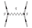
Figure 1: Amplitude of elastic scattering of two scalar nucleons (double solid lines) near the scalar pion (wavy line) pole $q^{2}=\mu^{2}$. In the vicinity of this pole the amplitude has the form $\mathcal{M}_{\chi\chi\to{}\chi\chi}={-g^{2}}/{(q^{2}-\mu^{2}+i0)}$.

For convenience, we introduce a dimensionless coupling constant

$$\alpha\equiv\frac{g^{2}}{16\pi m^{2}},$$ (4)

which appears as the coupling constant of the nonrelativistic Yukawa potential $U(r)=-\alpha e^{-\mu r}/r$ between two scalar nucleons. The electromagnetic interaction is not explicitly included into the Lagrangian (3) because it is assumed much weaker than the interaction between scalar nucleons and pions. We will need it only for the calculation of the nucleon electromagnetic form factor, where it will be taken into account perturbatively. In contrast to the electromagnetic fine structure constant $e^{2}$, the coupling constant $\alpha$ is not implied to be small and no expansions in it are used.

To regularize the theory, we introduce a PV scalar pion field $\varphi_{\textsc{pv}}$ with a large mass $\mu_{\textsc{pv}}\gg m,\,\mu$. The PV pion field is enough to regularize rather weak (logarithmic) divergences which appear in the scalar Yukawa model, i.e., there is no need to introduce an analogous PV nucleon field. Since PV fields have negative metric, the Lagrangian becomes

$$\mathscr{L}=\partial_{\nu}\chi^{\dagger}\partial^{\nu}\chi-m^{2}\chi^{\dagger}\chi+\delta m^{2}\chi^{\dagger}\chi+{\frac{1}{2}}\sum_{j=0}^{1}(-1)^{j}\big{[}\partial_{\nu}\varphi_{j}\partial^{\nu}\varphi_{j}-\mu^{2}_{j}\varphi^{2}_{j}\big{]}+\sum_{j=0}^{1}g_{0}\chi^{\dagger}\chi\varphi_{j},$$ (5)

where the index $j$ denotes a type of particle: the values $j=0$ and $j=1$ correspond, respectively, to the physical and PV scalar pion fields, $\mu_{0}\equiv\mu$, $\mu_{1}\equiv\mu_{\textsc{pv}}$. Similar procedure was used in Ref. Hiller98 .

Our main goal is to calculate the state vector $\phi(p)$ of the scalar nucleon. Then it can be used for calculating observables. The Fock space generated by the Lagrangian (3) embraces all Fock sectors composed of scalar nucleons, antinucleons, and pions. Each Fock sector contains one nucleon plus an arbitrary number of nucleon-antinucleon pairs plus arbitrary number of pions. It is known however that the contribution from the nucleon-antinucleon loops causes the instability of the vacuum Baym60 ; gross-tjon . We therefore truncate away all Fock sectors with antinucleons and construct a truncated Fock space from a set of Fock sectors with one scalar nucleon and increasing number of scalar pions. This procedure, however, comes with a penalty, as we will discuss below.

The introduction of PV scalar pions into the Lagrangian (5) extends the Fock space, which impacts the rule of particle counting inside Fock sectors. We postulate that PV scalar pions come to the theory on equal grounds with the physical ones. This means that any pion is counted as one particle, regardless to its type.

III State vector in Light-Front dynamics

The explicitly covariant form of LFD, as a more general approach mentioned in the Introduction, has many technical advantages in comparison with its noncovariant forms Carbonell98 . In particular, the four-vector $\omega$ serves as an indicator of possible dependence of calculated results on the light front orientation. This is especially important in approximate nonperturbative calculations, where such dependence may appear in calculated observables due to rotational symmetry breaking. For particles with spin, covariant LFD facilitates studying the spin structure of scattering amplitudes. In spite of these merits, for the case of scalar particles, these different forms of LFD are almost equivalent, even from the technical point of view. For this reason, we will not distinguish them below and, retaining in some instances the four-vector $\omega$ in explicit form, we will assume that it has definite components $(1,0,0,-1)$. If so, we have $\omega^{+}=0$, ${\mbox{\boldmath$\omega$}}_{\perp}={\bf 0}$, $\omega^{-}=2$, and $\omega\makebox[2.27626pt]{$\cdot$}a=a^{+}$ for an arbitrary four-vector $a$.

In LFD the state vector of a physical state is a solution of the eigenvalue equation (2) which can be written in an invariant form:

$$\hat{P}^{2}\phi(p)=M^{2}\phi(p),$$ (6)

where $\hat{P}^{2}=\hat{P}^{+}\hat{P}^{-}-{\hat{P}}^{2}_{\perp}$. The plus- and transverse components of the momentum operator in LFD do not contain the interaction; so they can be substituted, respectively, by the $p^{+}$ and ${\bf p}_{\perp}$ components of the total four-momentum $p$. The interaction is only contained in the minus-component of the momentum operator which can be represented as a sum of the free and interacting parts: ${\hat{P}}^{-}={\hat{P}}^{-}_{0}+\hat{P}_{\text{int}}^{-}$. The interacting part, in its turn, tightly relates to the light-front interaction Hamiltonian $\mathcal{H}_{\text{int}}(x)$:

$$\hat{P}^{-}_{\text{int}}=2\int\mathcal{H}_{\text{int}}(x)\delta(\omega\cdot x)d^{4}x=2\int_{{-\infty}}^{{+\infty}}\widetilde{\mathcal{H}}_{\text{int}}(\omega\tau)\frac{d\tau}{2\pi},$$ (7)

where $\widetilde{\mathcal{H}}_{\text{int}}$ is a Fourier transform of the interaction Hamiltonian:

$$\widetilde{\mathcal{H}}_{\text{int}}(\omega\tau)=\int\mathcal{H}_{\text{int}}(x)e^{-i(\omega\makebox[2.27626pt]{$\cdot$}x)\tau}d^{4}x.$$ (8)

In covariant form, the four-momentum operator can be written as

$$\hat{P}^{\nu}=\hat{P}_{0}^{\nu}+\omega^{\nu}\int_{{-\infty}}^{{+\infty}}\widetilde{\mathcal{H}}_{\text{int}}(\omega\tau)\frac{d\tau}{2\pi}.$$ (9)

Since $\omega^{2}=0$, we have $\omega\makebox[2.27626pt]{$\cdot$}\hat{P}=\omega\makebox[2.27626pt]{$\cdot$}\hat{P}_{0}=p^{+}$. In Ref. Bernard01 it was proven that the operators $\omega\makebox[2.27626pt]{$\cdot$}\hat{P}_{0}$ and $\hat{P}_{\text{int}}^{-}$ commute. We thus get

$$\hat{P}^{2}=\hat{P}_{0}^{2}+2p^{+}\int_{{-\infty}}^{{+\infty}}\widetilde{\mathcal{H}}_{\text{int}}(\omega\tau)\frac{d\tau}{2\pi}.$$ (10)

Substituting this result into Eq. (6), we finally obtain Bernard01

$$\left[\hat{P}_{0}^{2}-M^{2}\right]\phi(p)=-2p^{+}\int_{{-\infty}}^{{+\infty}}\widetilde{\mathcal{H}}_{\text{int}}(\omega\tau)\frac{d\tau}{2\pi}\,\phi(p).$$ (11)

The interaction Hamiltonian can be derived from the corresponding Lagrangian. We need the Hamiltonian in the interaction representation, i.e., that expressed through the free fields. For particles with spin or if the interaction depends on field derivatives the procedure may be, generally speaking, very nontrivial. The reason is that in LFD some of the equations of motion for field components are not dynamical equations but constraints. Exclusion of the non-dynamical degrees of freedom give rise to specific (contact) terms in the Hamiltonian. This point is explained in more detail in Ref. Karmanov04 . Fortunately, all that does not concern the case of scalar Yukawa model we consider here, because each scalar field has only one component. If so, one can simply identify the Hamiltonian with the interaction part of the Lagrangian taken with the opposite sign:

$$\mathcal{H}_{\text{int}}(x)=-g_{0}\,\chi^{\dagger}\chi\varphi-\delta m^{2}\chi^{\dagger}\chi.$$ (12)

To avoid overload with notations, we do not show explicitly the contribution of PV particles. They can be introduced later directly in the equations for the Fock components.

To solve Eq. (11), we make use of the Fock decomposition of the state vector $\phi(p)$, as given schematically by Eq. (1). We define the $n$-body Fock sector as a state containing one free scalar nucleon with the four-momentum $k_{1}$ plus $(n-1)$ free scalar pions with the four-momenta $k_{2},\ldots,k_{n}$. This state is obtained by acting with the corresponding creation operators on the vacuum:

$$|n\rangle=\hat{a}^{{\dagger}}({\bf k}_{1})\hat{c}^{{\dagger}}({\bf k}_{2})\ldots\hat{c}^{{\dagger}}({\bf k}_{n})|0\rangle.$$ (13)

The creation operators satisfy the standard commutation relation $[\hat{a}({\bf k}),\hat{a}^{{\dagger}}({\bf k}^{\prime})]=\delta^{(3)}({\bf k}-{\bf k}^{\prime})$ (for $\hat{c}$ and $\hat{c}^{{\dagger}}$ analogously). Due to the interaction, the total four-momentum $p$ of the physical nucleon is not equal to the sum of the constituent four-momenta: $k_{1}+\ldots+k_{n}\neq p$, i.e., momentum conservation is violated. Within LFD, only plus- and transverse components of the total four-momentum are conserved:

$$k_{1}^{+}+\ldots+k_{n}^{+}=p^{+},\,\,\,\,\,\,{\bf k}_{1\perp}+\ldots+{\bf k}_{n\perp}={\bf p}_{\perp}.$$ (14)

In the following, we will set ${\bf p}_{\perp}={\bf 0}$. This can be safely done due to the invariance of LFD with respect to transverse boosts. Using the four-vector $\omega$ introduced above, the relations (14) can be written in an explicitly covariant form which looks like the momentum conservation law:

$$k_{1}+\ldots+k_{n}=p+\omega\tau_{n}.$$ (15)

The scalar parameter $\tau_{n}$ (the off-shell light-front energy) can be expressed through the particle momenta by squaring both sides of Eq. (15):

$$\tau_{n}=\frac{s_{n}-M^{2}}{2p^{+}},$$ (16)

where $s_{n}$ is the invariant mass squared of the $n$-body Fock sector:

$$s_{n}\equiv(k_{1}+\ldots+k_{n})^{2}.$$ (17)

By definition, $s_{1}=m^{2}$. Note that $s_{n}$ is an eigenvalue of the free four-momentum operator squared $\hat{P}^{2}_{0}=p^{+}\hat{P}^{-}_{0}-p^{2}_{\perp}$:

$$\hat{P}^{2}_{0}|n\rangle=s_{n}|n\rangle.$$ (18)

The Fock decomposition of the physical scalar nucleon state vector can be written as Bernard01 :

$$\phi(p)=\sum_{n=1}^{\infty}\frac{2p^{+}(2\pi)^{3/2}}{(n-1)!}\int d\tau_{n}\left(\prod_{i=1}^{n}\frac{d^{3}k_{i}}{(2\pi)^{3/2}\sqrt{2\varepsilon_{k_{i}}}}\right)\,\psi_{n}(k_{1},\ldots k_{n};p)\,\delta^{(4)}(k_{1}+\ldots+k_{n}-p-\omega\tau_{n})\,|n\rangle,$$ (19)

where $\varepsilon_{k_{i}}=\sqrt{{\bf k}_{i}^{2}+m_{i}^{2}}$ and $m_{i}$ is the mass of the $i$-th constituent. All the four-momenta are on their mass shells, $k_{i}^{2}=m_{i}^{2}$. The combinatorial factor $1/(n-1)!$ takes into account the identity of scalar pions. The Dirac’s delta-function accounts for the four-momentum conservation law (15). Note that Eq. (19) may be considered as an exact definition of the light-front wave functions $\psi_{n}$.

The state vector satisfies the normalization condition

$${\phi^{{\dagger}}(p^{\prime})\phi(p)=2\varepsilon_{p}\delta^{(3)}({\bf p}-{\bf p}^{\prime})}$$ (20)

which reduces to

$$\sum_{n=1}^{\infty}I_{n}=1,$$ (21)

where

$$I_{n}=\frac{2p^{+}}{(2\pi)^{3(n-1)}(n-1)!}\int d\tau_{n}\left(\prod_{i=1}^{n}\frac{d^{3}k_{i}}{2\varepsilon_{k_{i}}}\right)|\psi_{n}(k_{1},\ldots,k_{n};p)|^{2}\delta^{(4)}(k_{1}+\ldots+k_{n}-p-\omega\tau_{n})$$ (22)

is the $n$-body Fock sector contribution to the full norm equal to unity. By its physical sense, $I_{n}$ is the probability that the physical state appears in the $n$-body Fock sector.

It is useful to introduce the light-front vertex functions $\Gamma_{n}$ related to the wave functions by

$$\Gamma_{n}\equiv(s_{n}-M^{2})\psi_{n}$$ (23)

and the new state vector

$${\cal G}(p)=2p^{+}\hat{\tau}\phi(p),$$ (24)

where the operator $\hat{\tau}$ acting on each Fock component $\psi_{n}$ yields $\tau_{n}\psi_{n}$. ${\cal G}(p)$ has the same Fock decomposition (19), changing the wave functions $\psi_{n}$ by the corresponding vertex functions $\Gamma_{n}$. Using Eqs. (18) and (16), and the definition (23), the main dynamical equation (11) for the state vector can be rewritten as Bernard01

$${\cal G}(p)=\frac{1}{2\pi}\int_{{-\infty}}^{{+\infty}}\left[-\widetilde{\mathcal{H}}_{\text{int}}(\omega\tau)\right]\,\frac{d\tau}{\tau}\,{\cal G}(p).$$ (25)

The vertex function $\Gamma_{n}$ is closely related to the full transition amplitude Hiller98 . This connection allows us to represent the system of equations for the vertex functions using the light-front time-ordered diagrams via the so-called covariant LFD graphical rules Carbonell98 . An $n$-body vertex diagram is shown in Fig. 2.

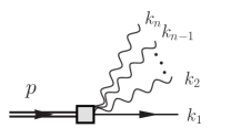
Figure 2: Diagram for the $n$-body vertex function $\Gamma_{n}(k_{1},k_{2},\ldots,k_{n};p)$. The scalar pions are represented by the wavy lines. The constituent and physical scalar nucleons are represented by the single and double straight lines, respectively.

For practical applications, it is convenient to transform the dependence of the wave and vertex functions on the constituent four-momenta $k_{1},\ldots,k_{n}$ into their dependence on the light-front variables which are the transverse momenta ${\bf k}_{i\perp}$ and the longitudinal momentum fractions $x_{i}\equiv k_{i}^{+}/p^{+}$ ($i=1,\ldots,n$). The $n$ pairs of the arguments $({\bf k}_{i\perp},x_{i})$ are constrained by the conditions

$$\sum_{i=1}^{n}x_{i}=1,\quad\sum_{i=1}^{n}{\bf k}_{i\perp}={\bf 0},$$ (26)

directly following from Eqs. (14). We thus have $(n-1)$ pairs of independent kinematical variables $({\bf k}_{i\perp},x_{i})$ in the $n$-body Fock sector. The invariant mass squared $s_{n}$ of the $n$-body Fock sector is expressed through the light-front variables as

$$s_{n}=\sum_{i=1}^{n}\frac{k^{2}_{i\perp}+m^{2}_{i}}{x_{i}}.$$ (27)

The dependence of the wave and vertex functions on the total four-momentum $p$ reduces to their dependence on $p^{2}=M^{2}$. It is convenient to exclude, by means of Eqs. (26), the scalar nucleon momenta ${\bf k}_{1\perp}$ and $x_{1}$ and to choose the scalar pion momenta as a set of independent variables. We thus write

$$\Gamma_{n}=\Gamma_{n}({\bf k}_{2\perp},x_{2},\ldots,{\bf k}_{n\perp},x_{n};M^{2})$$ (28)

and analogously for $\psi_{n}$. For simplicity, we will further suppress the dependence of Fock components on $M^{2}$ for the physical particle ($M^{2}=m^{2}$), whenever there is no danger of confusion.

IV Fock sector dependent renormalization

Fock sector dependent renormalization (FSDR) is a systematic scheme to renormalize light-front Hamiltonian field theory in truncated Fock space Karmanov08 . In this approach, the bare parameters (i.e., the full set of parameters entering into the interaction Hamiltonian and used for renormalization, such as bare coupling constants, bare masses, various counterterms, etc.) explicitly depend on the Fock sector, where they appear in the equations for the Fock components. For example, instead of the unique bare coupling constant $g_{0}$ one should assign to each interaction vertex in light-front diagrams the factor $g_{0l}$, where the index $l$ equals the difference between the order of Fock space truncation $N$ and the total number of other particles “in flight” at the instant which corresponds to the given vertex. The same concerns the mass counterterm $\delta m^{2}$. Actually, one has to deal with a whole series of bare coupling constants and mass counterterms being different for different Fock sectors:

$$g_{0}\;\to\;g_{0l},\quad\delta m^{2}\;\to\;\delta m^{2}_{l},\quad(l=1,2,\ldots,N).$$ (29)

In the general case, $l=(N-n_{s})$, where $n_{s}$ is the number of pion spectators. The assignment of the Fock sector dependence is illustrated in Fig. 3.

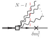
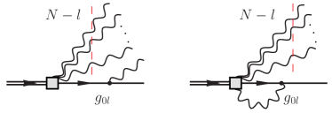
Figure 3: Assignment of Fock sector dependent bare parameters. Here $N$ is the maximal number of particles allowed by the truncation [one scalar nucleon plus $(N-1)$ scalar pions] and $N-l$ is the number of pion spectators which are intersected by the dashed line.

These sector dependent bare parameters can be determined successively, by increasing the order of truncation $N$. The trivial case $N=1$ yields $g_{01}=0$ and $\delta m^{2}_{1}=0$, since the only particle allowed is the scalar nucleon with no interactions and mass renormalization. Then, $g_{02}$ and $\delta m_{2}^{2}$ are determined in the two-body truncation ($N=2$), where the state vector is a superposition of the single scalar nucleon and one scalar nucleon plus one scalar pion Fock sectors. $g_{03}$ and $\delta m_{3}^{2}$ are determined in the three-body ($N=3$) truncation, where the scalar nucleon plus two scalar pions Fock sector is added. The bare parameters $g_{02}$ and $\delta m_{2}^{2}$ appearing in this approximation as well are used untouched, as they have been found from the $N=2$ case. The process repeats, until one’s desired Fock sector truncation is reached. Therefore, in order to find the state vector for the $N$-body truncation, one has to solve first the two-, three-, …, $(N-1)$-body problems. Below, to distinguish from each other the same quantities calculated in different approximations, we will supply the former ones by the superscript “$(N)$” indicating the order of Fock space truncation. Thus $\Gamma_{n}^{(N)}$ means the $n$-body vertex function found within the $N$-body Fock space truncation, $I_{n}^{(N)}$ stands for the $n$-body Fock sector norm obtained in the same approximation, etc.

The bare parameters relate to the physical ones by the renormalization conditions. The scalar nucleon mass counterterm is determined from the requirement that the physical and constituent nucleon masses coincide, i.e., $M=m$. In other words, one demands that the interaction does not change the nucleon mass. The bare coupling constant is obtained from the standard condition that the “dressed” two-body on-energy-shell vertex function turns into the physical coupling constant (see, e.g., Ref. Peskin95 ):

$$\sqrt{Z_{\chi}}\,\widetilde{\Gamma}_{2}^{\text{on-shell}}\sqrt{Z_{\chi}}\sqrt{Z_{\varphi}}=g,$$ (30)

where $Z$’s are the so-called field strength renormalization factors taking into account “radiative” corrections to the two-body vertex external legs and $\widetilde{\Gamma}$ denotes the two-body vertex amputated from all radiative corrections to its external legs. The factor $Z_{\chi}$ tightly relates to the corresponding scalar nucleon self-energy $\Sigma(p^{2})$ by

$$Z_{\chi}=\left[1{-}\Sigma^{\prime}(m^{2})\right]^{-1},$$ (31)

where the prime means the derivative

$$\Sigma^{\prime}(m^{2})\equiv\frac{\partial}{\partial p^{2}}\Sigma(p^{2})\Big{|}_{p^{2}=m^{2}}.$$ (32)

The self-energy is given by a sum of amplitudes of all irreducible diagrams with one-body initial and final states. For the scalar pion factor $Z_{\varphi}$ a formula analogous to Eq. (31) can be written down.

Note that the factorization of the “dressed” vertex into a product of the “bare” vertex $\widetilde{\Gamma}_{2}$ and the external leg factors $\sqrt{Z}$’s, which appears automatically in the four-dimensional Feynman approach, is a very nontrivial fact in the framework of LFD. First, such a factorization in LFD takes place on the energy shell only, while in the Feynman case it holds for the off-mass-shell vertex as well. Second, the factorization may be destroyed by approximations, e.g., the Fock space truncation. Fortunately, the LFD two-body vertex function enters into the renormalization condition (30) just being taken on the energy shell, where it coincides with the corresponding Feynman on-mass-shell two-body vertex. In addition, we do not consider here antinucleon contributions to the state vector, that leaves scalar pion a point-like particle, so that $Z_{\varphi}\equiv 1$. Under these conditions, one can safely accept Eq. (30) as a starting point of the bare coupling constant renormalization, even in truncated Fock space. Below we relate $\widetilde{\Gamma}_{2}$ to the previously introduced two-body vertex function $\Gamma_{2}$.

The condition that the nucleon-pion state is on the energy shell means that the constituent four-momenta satisfy the conservation law $k_{1}+k_{2}=p$ and, hence, $s_{2}=(k_{1}+k_{2})^{2}=m^{2}$. Going over to the light-front variables, we have $x_{1}+x_{2}=1$ and ${\bf k}_{1\perp}+{\bf k}_{2\perp}={\bf 0}$. So, the two-body vertex function depends on the two variables which we denote as

$$k_{\perp}\equiv|{\bf k}_{2\perp}|=|{\bf k}_{1\perp}|,\quad x\equiv x_{2}=1-x_{1}.$$ (33)

The invariant two-body mass squared in terms of these variables has the form

$$s_{2}=\frac{k_{\perp}^{2}+\mu^{2}}{x}+\frac{k_{\perp}^{2}+m^{2}}{1-x}.$$ (34)

On the energy shell, where $s_{2}=m^{2}$, we get

$$k_{\perp}=k_{\perp}^{*}(x)\equiv i\sqrt{m^{2}x^{2}+\mu^{2}(1-x)}$$ (35)

(the choice of the sign, $+i\sqrt{\vphantom{m}\ldots}$ or $-i\sqrt{\vphantom{m}\ldots}$, is not important, since the two-body vertex function depends in fact on $k_{\perp}^{2}$) and

$$\widetilde{\Gamma}_{2}^{\text{on-shell}}=\widetilde{\Gamma}_{2}(s_{2}=m^{2})=\widetilde{\Gamma}_{2}(k_{\perp}^{*}(x),x).$$ (36)

Since the field strength renormalization factors are constants (i.e., they do not depend on any kinematical variables), the renormalization condition (30) implies that the two-body vertex function taken on the energy shell must turn into a constant too. This is indeed so in perturbation theory. It would be true in exact nonperturbative calculations, if they were possible. In approximate nonperturbative approach however such a property is not automatically guaranteed and the calculated two-body vertex keeps $x$-dependence even on the energy shell. If so, one may consider Eq. (30) to be true for some particular value of $x=x^{*}$ only, choosing $x^{*}$ at our own will Karmanov10 ; Mathiot11 . An evident flaw here is the dependence of calculated observables on the extra nonphysical parameter $x^{*}$. Since there are not any strict arguments in favor of some preset value $x^{*}$, whether this dependence is weak or not is a matter of chance. An alternative way proposed in Ref. Karmanov12 seems more justified. It demands Eq. (30) to be true for all $0\leq x\leq 1$, but admits $x$-dependence of the bare parameters, uniquely determined directly from the system of equations for the Fock components. Now the nonphysical dependence of the on-energy-shell two-body vertex function on kinematical variables, caused by the Fock space truncation, shifts to unobserved quantities, while the renormalization condition (30) becomes fully self-consistent. One may also expect that this method improves the stability of calculated observables as a function of the regularization parameters (PV masses), as, e.g., the calculations of the spin-1/2 fermion anomalous magnetic moment in the Yukawa model, obtained in Ref. Karmanov12 , show.

We emphasize: by making a truncation, we approximate the initial field-theoretical Hamiltonian by a matrix of finite dimension (in terms of the particle number), acting in Fock space. This is the reason, why in “new” dynamics the on-shell two-body vertex function (36) calculated with constant bare parameters acquires dependence on the variable $x$. Assuming appropriate $x$-dependence of the bare coupling constant which implicitly enters into $\widetilde{\Gamma}_{2}^{\text{on-shell}}$ allows the latter to be $x$-independent. So, $x$-dependence of bare parameters compensates, to some extent, the effect of missed (because of the Fock space truncation) contributions. In Sec. VIII below, by using an example, we will demonstrate explicitly that after taking into account the contribution eliminated by truncation the $x$-dependence of the on-shell two-body vertex function does completely disappear.

Upon adoption within a truncated Fock space, the general renormalization condition (30) should be reformulated according to the FSDR requirements. The factor $\sqrt{Z_{\chi}}$ in front of $\widetilde{\Gamma}_{2}^{\text{on-shell}}$ comes from the “dressing” of a single scalar nucleon line. For the Fock space truncation of order $N$ it should be thus substituted by $\sqrt{Z_{\chi}^{(N)}}$. The analogous factor behind $\widetilde{\Gamma}_{2}^{\text{on-shell}}$ corresponds to the “dressing” of a scalar nucleon line in the two-body (nucleon plus pion) state. Since the total number of particles in any Fock sector can not exceed $N$, this factor should be calculated in the lower $(N-1)$ approximation. Taking into account that $\sqrt{Z_{\varphi}}\equiv 1$, we obtain

$$\sqrt{Z_{\chi}^{(N)}}\,\widetilde{\Gamma}^{{(N)}}_{2}(s_{2}=m^{2})\sqrt{Z_{\chi}^{(N-1)}}=g.$$ (37)

To make practical use of Eq. (37) one should relate the “amputated” two-body vertex $\widetilde{\Gamma}_{2}$ to the previously introduced two-body Fock component $\Gamma_{2}$. This relation has the form Karmanov10

$$\Gamma_{2}^{{(N)}}(s_{2}=m^{2})=\sqrt{I_{1}^{(N)}}\widetilde{\Gamma}_{2}^{{(N)}}(s_{2}=m^{2})Z_{\chi}^{(N-1)},$$ (38)

where $I_{1}^{(N)}$ is the one-body Fock sector normalization integral in the $N$-body truncated Fock space. Its calculation according to Eq. (22) yields $I_{1}^{(N)}=|\psi_{1}^{(N)}|^{2}$. Note that the normalization condition (21) for the state vector now acquires the form

$$\sum_{n=1}^{N}I_{n}^{(N)}=1.$$ (39)

In terms of the light-front variables, $I_{n}^{(N)}$ is expressed through the corresponding vertex function as

$$I_{n}^{(N)}=\frac{2}{(2\pi)^{3(n-1)}(n-1)!}\int\prod_{i=1}^{n}\frac{d^{2}k_{i\perp}dx_{i}}{2x_{i}}\,\left[\frac{\Gamma_{n}^{(N)}}{s_{n}-M^{2}}\right]^{2}\,\delta^{(2)}\left(\sum_{i=1}^{n}{\bf k}_{i\perp}\right)\delta\left(\sum_{i=1}^{n}x_{i}-1\right).$$ (40)

In Ref. Karmanov10 it was proven that the field strength renormalization factor for a spin-1/2 fermion exactly coincides with the corresponding one-body normalization integral. The proof can be easily reduced to the scalar case. Applying this result to the quantities in truncated Fock space means

$$Z_{\chi}^{(N)}=I_{1}^{(N)}.$$ (41)

Combining Eqs. (37), (38), and (41) together gives the final form of the renormalization condition for the bare coupling constant:

$$\Gamma_{2}^{(N)}(s_{2}=m^{2})=g\sqrt{I_{1}^{(N-1)}}.$$ (42)

On introducing PV particles, one has to supply the vertex functions with additional indices pointing out the types of scalar pions in the corresponding Fock sectors. We will denote the pion type by the superscript $j_{l}$, $l=2,\,3,\ldots,\,n$:

$$\Gamma_{n}^{(N)}({\bf k}_{2\perp},x_{2},\ldots,{\bf k}_{n\perp},x_{n})\to\Gamma_{n}^{(N)j_{2}\ldots j_{n}}({\bf k}_{2\perp},x_{2},\ldots,{\bf k}_{n\perp},x_{n}).$$

According to the notations accepted in Sec. II, $j_{l}=0$ stands for a physical pion, while $j_{l}=1$ corresponds to a PV one. The renormalization condition (42) is imposed on the physical component $\Gamma_{2}^{(N)j_{2}=0}$ of the two-body vertex.

V Scalar nucleon state vector in the two-body ($N=2$) truncation

V.1 Equations for the Fock components and their solution

In the two-body truncation, we keep up to two particles (one scalar nucleon plus one scalar pion) in the Fock space. The system of equations for the vertex functions, obtained from the general equation (25) for the state vector, is shown graphically in Fig. 4.

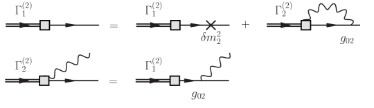
Figure 4: System of equations for the vertex functions in the two-body truncation.

The rules of the LFD graph techniques are exposed, in covariant form, e.g., in Ref. Carbonell98 . Applying them to the system of equations considered, one gets

$$\Gamma_{1}^{(2)}\;=\;\; \delta m^{2}_{2}\frac{\Gamma^{(2)}_{1}}{m^{2}-M^{2}}+g_{02}\sum_{j=0}^{1}(-1)^{j}\int_{0}^{1}\frac{dx}{2x(1-x)}\int\frac{d^{2}k_{\perp}}{(2\pi)^{3}}\frac{\Gamma_{2}^{(2)j}(k_{\perp},x)}{s_{2}^{j}-M^{2}},$$ (43)

$$\Gamma^{(2)j}_{2}(k_{\perp},x)\;=\;\; g_{02}\frac{\Gamma^{(2)}_{1}}{m^{2}-M^{2}},$$ (44)

where

$$s_{2}^{j}=\frac{k^{2}_{\perp}+\mu^{2}_{j}}{x}+\frac{k^{2}_{\perp}+m^{2}}{1-x}$$ (45)

is the invariant mass squared of the two-body state made from the one scalar nucleon and one scalar pion of the $j$-th type [cf. with Eq. (34)]. The arguments of the two-body vertex function are defined by Eqs. (33). The factor $(-1)^{j}$ takes into account the negative norm of the PV scalar pion. Note that $\Gamma^{(2)}_{1}/(m^{2}-M^{2})=\psi_{1}^{(2)}$ is a constant in the sense that it does not depend on kinematical variables. The bare parameters are assigned to the vertices of the diagrams, according to the FSDR requirements. This is the reason why Eq. (44) does not contain, on its right-hand side, a contribution from the scalar nucleon mass counterterm. In principle, one should add such a contribution (it is shown in Fig. 5), because it is generated by the interaction Hamiltonian (12). At the same time, within the two-body truncation, one has to assign the factor $\delta m_{1}^{2}$ to the corresponding vertex given by the mass counterterm, since there is already one scalar pion in flight in the two-body state. Due to the fact that $\delta m_{1}^{2}=0$, the diagram in Fig. 5 does not contribute to Eq. (44).

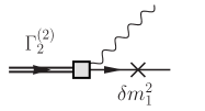
Figure 5: Contribution from the mass counterterm, which is absent in the two-body truncation.

In the limit $M\to m$ the one-body vertex function $\Gamma_{1}^{(2)}\sim(m^{2}-M^{2})\to 0$, while $\psi_{1}^{(2)}$ has a constant value determined from the normalization condition (39) for the state vector. The system of equations (43) and (44) thus reduces to

$$0\;=\;\; \delta m^{2}_{2}\psi_{1}^{(2)}\ {-}g_{02}^{2}\bar{\Sigma}^{(2)}(m^{2})\psi_{1}^{(2)},$$ (46)

$$\Gamma^{(2)j}_{2}(k_{\perp},x)\;=\;\; g_{02}\psi_{1}^{(2)},$$ (47)

where $\bar{\Sigma}^{(2)}$ is nothing but the scalar nucleon self-energy in the two-body approximation, $\Sigma^{(2)}$, amputated from the coupling constant squared. For an arbitrary value of its argument $p^{2}$, this function is given by

$$\bar{\Sigma}^{(2)}(p^{2})={-}\sum_{j=0}^{1}(-1)^{j}\int_{0}^{1}\frac{dx}{2x(1-x)}\int\frac{d^{2}k_{\perp}}{(2\pi)^{3}}\frac{1}{s_{2}^{j}-p^{2}}.$$ (48)

By definition, $\bar{\Sigma}^{(2)}(p^{2})=\Sigma^{(2)}(p^{2})/g_{02}^{2}$. It enters into Eq. (46) at $p^{2}=m^{2}$. When the PV scalar pion mass $\mu_{1}$ tends to infinity, $\bar{\Sigma}^{(2)}(p^{2})$ diverges like $\log(\mu_{1}/m)$. The function $\bar{\Sigma}^{(2)}(p^{2})$ is calculated in an explicit form in Appendix A.

Equation (46) determines the mass counterterm:

$$\delta m_{2}^{2}={g_{02}^{2}\bar{\Sigma}^{(2)}(m^{2})},$$ (49)

while $\psi_{1}^{(2)}$ still remains a free constant. $\delta m_{2}^{2}$ is not immediately needed for the two-body truncation and will be analyzed later. The two-body vertex function, as follows from Eq. (47), is a constant too: it depends neither on kinematical variables nor on the index $j$. This fact is a direct consequence of the two-body Fock space truncation and, generally speaking, it does not hold in higher order truncations. The renormalization condition (42) at $N=2$ reads simply

$$\Gamma_{2}^{(2)j=0}(k^{*}_{\perp}(x),x)=g,$$ (50)

where we have used $I_{1}^{(1)}=1$ (free theory). Since $\Gamma_{2}^{(2)j}(k_{\perp},x)\equiv\Gamma_{2}^{(2)}$ is a constant, one gets

$$\Gamma_{2}^{{(2)}}=g.$$ (51)

The one-body wave function $\psi_{1}^{(2)}$ is now defined by the state vector normalization:

$$\psi_{1}^{(2)}=\sqrt{I_{1}^{(2)}}=\sqrt{1-I_{2}^{(2)}},$$ (52)

where

$$I_{2}^{(2)} = {\sum_{j=0}^{1}(-1)^{j}\int_{0}^{1}\frac{dx}{2x(1-x)}\int\frac{d^{2}k_{\perp}}{(2\pi)^{3}}\left[\frac{\Gamma_{2}^{(2)}}{s_{2}^{j}-m^{2}}\right]^{2}}$$ (53)

$$= {\frac{g^{2}}{16\pi^{2}m^{2}}}\int_{0}^{1}dx\bigg{[}\frac{x(1-x)}{(1-x)\mu^{2}/m^{2}+x^{2}}-\frac{x(1-x)}{(1-x)\mu^{2}_{1}/m^{2}+x^{2}}\bigg{]}.$$

The two-body Fock sector norm $I_{2}^{(2)}$ (and, hence, $I_{1}^{(2)}$) is finite even after removing the ultraviolet regulator, i.e., at $\mu_{1}\to\infty$. It is convenient to introduce the two-body norm $\bar{I}_{2}^{(2)}$ amputated from the coupling constant squared. By definition, $\bar{I}_{2}^{(2)}=I_{2}^{(2)}/g^{2}$. It does not depend on $g$. Note that the following identity is valid:

$$\bar{I}_{2}^{(2)}={-}{\bar{\Sigma}^{(2)}}{{}^{\prime}}(m^{2}).$$ (54)

This result can be checked by differentiating the right-hand side of Eq. (48) and comparing the result with the right-hand side of Eq. (53). The derivative ${\bar{\Sigma}^{(2)}}{{}^{\prime}}(m^{2})$ is calculated analytically in Appendix A. Now we obtain for the one-body wave function

$$\psi_{1}^{(2)}=\sqrt{1-g^{2}\bar{I}_{2}^{(2)}}.$$ (55)

Eqs. (51) and (55) determine the normalized (and renormalized) Fock components of the scalar nucleon state vector in the two-body truncation.

The two-body wave function is

$$\begin{split}\psi_{2}^{(2)j}(k_{\perp},x)=\frac{\Gamma_{2}^{(2)}}{s_{2}^{j}-m^{2}}=\frac{gx(1-x)}{k_{\perp}^{2}+\mu_{j}^{2}(1-x)+m^{2}x^{2}}.\end{split}$$ (56)

In contrast to the vertex function, it depends on both kinematical variables and on the index $j$.

V.2 Renormalization Parameters

To fix all the renormalization parameters, one should relate the bare coupling constant $g_{02}$ with the physical one. Once the Fock components are available, the relation desired can be obtained from Eq. (47):

$$g_{02}=\frac{g}{\psi_{1}^{(2)}}=\frac{g}{\sqrt{1-{g^{2}\bar{I}_{2}^{(2)}}}}.$$ (57)

Substituting Eq. (57) into Eq. (49), we find the mass counterterm:

$$\delta m_{2}^{2}={\frac{g^{2}\bar{\Sigma}^{(2)}(m^{2})}{1-g^{2}{\bar{I}_{2}^{(2)}}}}.$$ (58)

Then, the field strength renormalization factor defined by Eq. (31),

$$Z^{(2)}_{\chi}={\left[1{-}g_{02}^{2}{\bar{\Sigma}^{(2)}}{{}^{\prime}}(m^{2})\right]^{-1}=1{+}g^{2}{\bar{\Sigma}^{(2)}}{{}^{\prime}}(m^{2})=1-I_{2}^{(2)}}=I_{1}^{(2)},$$ (59)

as expected. In the limit of infinite PV scalar pion mass $\mu_{1}$ the quantities $g_{02}$ and $Z_{\chi}^{{(2)}}$ tend to finite values, while $\delta m_{2}^{2}$ diverges logarithmically, like the self-energy $\bar{\Sigma}^{(2)}$. The bare parameters $g_{02}$ and $\delta m_{2}^{2}$ defined by Eqs. (57) and (58), respectively, will be used as an input in the next order ($N=3$) approximation.

V.3 Critical coupling associated with the Landau pole

From Eq. (57) it is seen that $g_{02}^{2}$ considered as a function of $g^{2}$ becomes singular at $g^{2}=1/\bar{I}_{2}^{(2)}$. A similar singularity arises in the bare coupling of QED and is called the Landau pole. The critical coupling constant $\alpha=\alpha_{\textsc{l}}$ associated with the Landau pole is determined by

$$\alpha_{\textsc{l}}^{-1}={16\pi m^{2}\bar{I}_{2}^{(2)}=\frac{1}{\pi}}\int_{0}^{1}dx\bigg{[}\frac{x(1-x)}{(1-x)\mu^{2}/m^{2}+x^{2}}-\frac{x(1-x)}{(1-x)\mu^{2}_{1}/m^{2}+x^{2}}\bigg{]},$$ (60)

where $\alpha$ relates to $g$ by Eq. (4). If $\alpha>\alpha_{\textsc{l}}$, the bare coupling constant $g_{02}$ becomes imaginary. In principle, one can always adjust the PV scalar pion mass $\mu_{1}$ to make $\alpha_{\textsc{l}}$ large enough for the mathematical self-consistency of the model. From physical considerations however it is evident that one has to take $\mu_{1}\gg m$ to claim that the renormalization procedure allows one to eliminate the regularization parameters. In the limit $\mu_{1}\to\infty$ Eq. (60) reduces to

$$\alpha_{\textsc{l}}=\pi\left[\frac{\xi(3-\xi^{2})}{\sqrt{4-\xi^{2}}}\,\arctan\left(\frac{\sqrt{4-\xi^{2}}}{\xi}\right)-1+(1-\xi^{2})\log\frac{1}{\xi}\right]^{-1},$$ (61)

where $\xi=\mu/m$. For $\mu/m=0.14/0.94$, $\alpha_{\textsc{l}}\simeq 2.630$. Above the critical coupling, the scalar Yukawa theory becomes ill-defined. At the same time, the threshold of the coupling constant may not be apparent in calculated observables within the two-body truncation, which are well-defined for arbitrary strong coupling. The critical coupling (61) however brings real restrictions on admitted values of $\alpha$ in the three-body truncation, where the renormalized Fock components do not exist at $\alpha>\alpha_{\textsc{l}}$. We will discuss these points in more detail below.

VI Scalar nucleon state vector in the three-body ($N=3$) truncation

VI.1 Equations for the Fock components and their solution

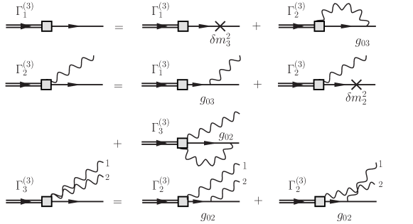
Figure 6: System of equations for the Fock components in the three-body truncation.

The system of equations for the vertex functions in the three-body Fock space truncation ($N=3$) is graphically shown in Fig. 6. It differs from that in the $N=2$ case by the presence of three-body intermediate states which complicate the equations to some extent. According to the FSDR rules Karmanov08 , the elementary interaction vertices inside full three-body states, (i.e., the vertices appearing simultaneously with a scalar pion spectator), contain the bare coupling constant $g_{02}$ or the mass counterterm $\delta m^{2}_{2}$. The interaction vertices with no pion spectator above them correspond to the factors $g_{03}$ or $\delta m_{3}^{2}$. The appearance, in different intermediate states, of the sector dependent bare coupling constants, either $g_{02}$ or $g_{03}$, and the mass counterterms, either $\delta m_{2}^{2}$ or $\delta m_{3}^{2}$, is the very essence of the sector dependent renormalization scheme.

When we solve the problem in the three-body truncation, the values $g_{02}$ and $\delta m^{2}_{2}$ are assumed to be known — they were obtained in the two-body truncation [see Eqs. (57) and (58)]. The new renormalization parameters $g_{03}$ and $\delta m_{3}^{2}$ will be found by applying the renormalization conditions again. So, in the framework of FSDR, the refinement of these quantities from sector to sector is analogous to their refinement, from order to order, in perturbation theory. As explained in Sec. IV, we need the sector dependent renormalization scheme in order to eliminate divergences for any given truncation.

Applying the rules of the LFD graph techniques, we cast the system of equations for the vertex functions in the three-body truncation in an analytical form:

$$\Gamma_{1}^{(3)}\;=\;\; \frac{\delta m^{2}_{3}\,\Gamma^{(3)}_{1}}{m^{2}-M^{2}}+g_{03}\sum_{j=0}^{1}(-1)^{j}\int_{0}^{1}\frac{dx}{2x(1-x)}\int\frac{d^{2}k_{\perp}}{(2\pi)^{3}}\frac{\Gamma_{2}^{(3)j}(k_{\perp},x)}{{{s}_{2}^{j}}-M^{2}},$$ (62)

$$\Gamma^{(3)j}_{2}(k_{\perp},x)\;=\;\; \frac{g_{03}\,\Gamma^{(2)}_{1}}{m^{2}-M^{2}}+\frac{\delta m_{2}^{2}\,\Gamma^{(3)j}_{2}(k_{\perp},x)}{{(1-x)}({s_{2}^{j}}-M^{2})}$$

$$+ g_{02}\sum_{\mathclap{j^{\prime}=0}}^{1}(-1)^{j^{\prime}}\int\limits_{0}^{\mathclap{1-x}}\frac{dx^{\prime}}{2x^{\prime}(1-x-x^{\prime})}\int\frac{d^{2}k^{\prime}_{\perp}}{(2\pi)^{3}}\frac{\Gamma_{3}^{(3)jj^{\prime}}(k_{\perp},x,k^{\prime}_{\perp},x^{\prime})}{{s_{3}^{jj^{\prime}}}-M^{2}},$$ (63)

$$\Gamma_{3}^{(3){jj^{\prime}}}({k_{\perp},x,k^{\prime}_{\perp},x^{\prime}})\;=\;\; \frac{g_{02}\,\Gamma_{2}^{(3){j}}({k_{\perp},x})}{(1-{x})({s_{2}^{j}}-M^{2})}+\frac{g_{02}\,\Gamma_{2}^{(3){j}}({k^{\prime}_{\perp},x^{\prime}})}{(1-{x^{\prime}})({{s^{\prime}}_{2}^{j^{\prime}}}-M^{2})},$$ (64)

where $s_{2}^{j}$ is defined by Eq. (45), ${s^{\prime}}_{2}^{j^{\prime}}$ is given by the same formula, changing $k_{\perp}\to k^{\prime}_{\perp}$, $x\to x^{\prime}$, and $j\to j^{\prime}$, and

$$s_{3}^{jj^{\prime}}=\frac{k^{2}_{\perp}+\mu^{2}_{j}}{x}+\frac{{k^{\prime}}^{2}_{\perp}+\mu^{2}_{j^{\prime}}}{x^{\prime}}+\frac{({\bf k}_{\perp}+{\bf k}^{\prime}_{\perp})^{2}+m^{2}}{1-x-x^{\prime}}$$ (65)

is the three-body invariant mass squared.

As before, the mass eigenvalue $M$ is implied to be identical to the physical nucleon mass $m$, i.e., the limit $M\to m$ should be taken in Eqs. (62)–(64). The three-body vertex function $\Gamma_{3}^{{(3)}}$ is expressed through the two-body vertex. Therefore, it can be excluded by substituting Eq. (64) into Eq. (63). The corresponding analytical expression reads

$$\bigg{[}1-\frac{g_{02}^{2}\bar{\Sigma}^{(2)}(\ell^{2}){-}\delta m_{2}^{2}}{\ell^{2}-m^{2}}\bigg{]}\Gamma^{(3)j}_{2}({k}_{\perp},x)=g_{03}\psi_{1}^{(3)}+g_{02}^{2}\sum_{j^{\prime}=0}^{1}(-1)^{j^{\prime}}\int\limits_{0}^{\mathclap{1-x}}\frac{dx^{\prime}}{2x^{\prime}(1-x^{\prime})(1-x-x^{\prime})}\int\frac{d^{2}k^{\prime}_{\perp}}{(2\pi)^{3}}\\ \times\frac{\Gamma^{(3)j^{\prime}}_{2}(k^{\prime}_{\perp},x^{\prime})}{({s^{\prime}}_{2}^{j^{\prime}}-m^{2})(s_{3}^{jj^{\prime}}-m^{2})}.$$ (66)

where $\ell^{2}=m^{2}-(1-x)({s_{2}^{j}-m^{2}})$. The term proportional to the self-energy $\bar{\Sigma}^{(2)}(\ell^{2})$ is generated by the substitution of the first addendum on the right-hand side of Eq. (64) into the integral term of Eq. (63). Indeed, the result of this substitution has the form

$$\frac{g_{02}^{2}\Gamma_{2}^{(3)j}(k_{\perp},x)}{(1-x)(s_{2}^{j}-m^{2})}\,\sum_{j^{\prime}=0}^{1}(-1)^{j^{\prime}}\int_{0}^{1-x}\frac{dx^{\prime}}{2x^{\prime}(1-x-x^{\prime})}\int\frac{d^{2}k_{\perp}^{\prime}}{(2\pi)^{3}}\,\frac{1}{s_{3}^{jj^{\prime}}-m^{2}}.$$ (67)

Making the sequential change of the integration variables $x^{\prime}\to(1-x)x^{\prime}$ and then ${\bf k}^{\prime}_{\perp}\to{\bf k}_{\perp}^{\prime}-x^{\prime}{\bf k}_{\perp}$, we can cast the expression (67) in the form

$$\frac{g_{02}^{2}\Gamma_{2}^{(3)j}(k_{\perp},x)}{(1-x)(s_{2}^{j}-m^{2})}\,\sum_{j^{\prime}=0}^{1}(-1)^{j^{\prime}}\int_{0}^{1}\frac{dx^{\prime}}{2x^{\prime}(1-x^{\prime})}\int\frac{d^{2}k_{\perp}^{\prime}}{(2\pi)^{3}}\,\frac{1}{{s^{\prime}}_{2}^{j^{\prime}}-{\ell^{2}}}=\frac{g_{02}^{2}\Gamma_{2}^{(3)j}(k_{\perp},x)\bar{\Sigma}^{(2)}(\ell^{2})}{{\ell^{2}}-m^{2}},$$ (68)

as follows from Eq. (48) and the definition of the quantity $\ell^{2}$. The latter is nothing else than the square of the off-shell four-momentum of the constituent scalar nucleon in the two-body state: $\ell^{2}=(p-k_{2})^{2}$, where $k_{2}$ is the scalar pion spectator four-momentum. Note that both the self-energy $g_{02}^{2}\bar{\Sigma}^{(2)}(\ell^{2})$ and the mass counterterm $\delta m_{2}^{2}$ diverge logarithmically at large mass $\mu_{1}$ of the PV scalar pion, but their combination

$$g_{02}^{2}\bar{\Sigma}^{(2)}(\ell^{2}){-}\delta m_{2}^{2}=g_{02}^{2}\left[\bar{\Sigma}^{(2)}(\ell^{2})-\bar{\Sigma}^{(2)}(m^{2})\right]$$ (69)

entering into Eq. (66) is finite in this limit, provided $\ell^{2}$ is of order of physical masses squared. This cancellation of divergent terms is just an important feature of FSDR. The equation (66) determining the two-body vertex function $\Gamma^{(3)j}_{2}(k_{\perp},x)$ in the three-body truncation is a three-body counterpart of Eq. (47). When $k_{\perp}\to\infty$, it turns into $\Gamma^{(3)j}_{2}\to g_{03}\psi_{1}^{{(3)}}$, which differs from $\Gamma_{2}^{(2)j}$ by the replacement of the index pointing out the order of truncation.

The substitution of Eq. (64) into Eq. (63), which has been done analytically, could be realized diagrammatically as well. In such a way, we would obtain the graphical equation for the two-body vertex function, shown in Fig. 7. Using the LFD graph techniques rules leads to the same analytical equation (66).

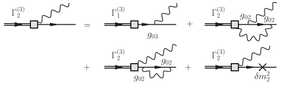
Figure 7: Equation for the two-body component after the exclusion of the three-body component.

Now we make use of Eqs. (57), (54), and (58) in order to get rid of the second order bare parameters $g_{02}$ and $\delta m_{2}^{2}$ in Eq. (66). After simple transformations, we arrive at the following equation

$$\left[1-\frac{g^{2}\bar{\Sigma}_{r}^{(2)}(\ell^{2})}{\ell^{2}-m^{2}}\right]\Gamma_{2}^{(3)j}(k_{\perp},x) = g_{03}\psi_{1}^{(3)}\left[1-g^{2}\bar{I}_{2}^{(2)}\right]$$

$$+\frac{g^{2}}{8\pi^{2}}\sum_{j^{\prime}=0}^{1}(-1)^{j^{\prime}}\int_{0}^{1-x}dx^{\prime}\int_{0}^{\infty}dk_{\perp}^{\prime}\,k_{\perp}^{\prime}\,V^{jj^{\prime}}(k_{\perp},x,k_{\perp}^{\prime},x^{\prime})\Gamma_{2}^{(3)j^{\prime}}(k_{\perp}^{\prime},x^{\prime}),$$

where

$$\bar{\Sigma}_{r}^{(2)}(\ell^{2})=\bar{\Sigma}^{(2)}(\ell^{2})-\bar{\Sigma}^{(2)}(m^{2})-\bar{\Sigma}^{(2)}{{}^{\prime}}(m^{2})(\ell^{2}-m^{2})$$ (71)

is the renormalized scalar nucleon self-energy in the two-body truncation, its argument

$$\ell^{2}=-\frac{k_{\perp}^{2}}{x}+(1-x)m^{2}-\mu_{j}^{2}\left(\frac{1-x}{x}\right),$$ (72)

and

$$V^{jj^{\prime}}(k_{\perp},x,k_{\perp}^{\prime},x^{\prime}) = \frac{1}{2\pi x^{\prime}(1-x^{\prime})(1-x-x^{\prime})({s^{\prime}}_{2}^{j^{\prime}}-m^{2})}\int_{0}^{2\pi}\frac{d\phi^{\prime}}{s_{3}^{jj^{\prime}}-m^{2}}$$ (73)

$$= \frac{1}{{k^{\prime}}^{2}_{\perp}+\mu_{j^{\prime}}^{2}(1-x^{\prime})+m^{2}{x^{\prime}}^{2}}$$

$$\times\left[(1-x-x^{\prime})^{2}\left(\frac{k_{\perp}^{2}+\mu_{j}^{2}}{x}+\frac{{k^{\prime}}^{2}_{\perp}+\mu_{j^{\prime}}^{2}}{x^{\prime}}+\frac{k_{\perp}^{2}+{k^{\prime}}^{2}_{\perp}+m^{2}}{1-x-x^{\prime}}-m^{2}\right)^{2}-4k_{\perp}^{2}{k^{\prime}}^{2}_{\perp}\right]^{-1/2}.$$

The integration over the azimuthal angle $\phi^{\prime}$ has been done analytically by using the formula

$$\int\limits_{0}^{2\pi}\frac{d\phi^{\prime}}{A+B\cos\phi^{\prime}}=\frac{2\pi}{\sqrt{A^{2}-B^{2}}},\qquad(A^{2}>B^{2}).$$ (74)

Eq. (LABEL:G2f) contains the undefined bare coupling constant $g_{03}$. To fix it, one should apply the renormalization condition (42) which now becomes

$$\Gamma_{2}^{(3)j=0}(k^{*}_{\perp}(x),x)=g\sqrt{I_{1}^{(2)}}=g\sqrt{1-g^{2}\bar{I}_{2}^{(2)}}$$ (75)

with $k^{*}_{\perp}(x)$ given by Eq. (35). We thus set $k_{\perp}=k^{*}_{\perp}(x)$ and $j=0$ on both sides of Eq. (LABEL:G2f) and demand the condition (75) to hold for arbitrary $0\leq x\leq 1$. The argument of the self-energy $\ell^{2}$ turns into $m^{2}$ at the renormalization point. Taking into account that

$$\bar{\Sigma}_{r}^{(2)}(\ell^{2})\stackrel{{\scriptstyle\ell^{2}\to m^{2}}}{{\sim}}(\ell^{2}-m^{2})^{2},$$

we get

$$g_{03}\psi_{1}^{(3)} = \left[1-g^{2}\bar{I}_{2}^{(2)}\right]^{-1}$$ (76)

$$\times\left[g\sqrt{1-g^{2}\bar{I}_{2}^{(2)}}-\frac{g^{2}}{8\pi^{2}}\sum_{j^{\prime}=0}^{1}(-1)^{j^{\prime}}\int_{0}^{1-x}dx^{\prime}\int_{0}^{\infty}dk_{\perp}^{\prime}\,k_{\perp}^{\prime}\,V^{0j^{\prime}}(k^{*}_{\perp}(x),x,k_{\perp}^{\prime},x^{\prime})\Gamma_{2}^{(3)j^{\prime}}(k_{\perp}^{\prime},x^{\prime})\right].$$

An immediate observation is that the right-hand side of Eq. (76) depends on the longitudinal momentum fraction of the scalar pion $x$. Therefore, we allow $g_{03}$ to depend on $x$ in order to satisfy the condition Eq. (75) for any value of $x$ Karmanov12 (see the detailed discussion below, in Sec. VIII). Substituting the combination $g_{03}\psi_{1}^{(3)}$ back into Eq. (LABEL:G2f), we find a closed renormalized equation for the two-body vertex function:

$$\left[1-\frac{g^{2}\bar{\Sigma}_{r}^{(2)}(\ell^{2})}{\ell^{2}-m^{2}}\right]\Gamma_{2}^{(3)j}(k_{\perp},x) = g\sqrt{1-g^{2}\bar{I}_{2}^{(2)}}$$

$$+\frac{g^{2}}{8\pi^{2}}\sum_{j^{\prime}=0}^{1}(-1)^{j^{\prime}}\int_{0}^{1-x}dx^{\prime}\int_{0}^{\infty}dk_{\perp}^{\prime}\,k_{\perp}^{\prime}\,\Delta V^{jj^{\prime}}(k_{\perp},x,k_{\perp}^{\prime},x^{\prime})\Gamma_{2}^{(3)j^{\prime}}(k_{\perp}^{\prime},x^{\prime}),$$

where

$$\Delta V^{jj^{\prime}}(k_{\perp},x,k_{\perp}^{\prime},x^{\prime})=V^{jj^{\prime}}(k_{\perp},x,k_{\perp}^{\prime},x^{\prime})-V^{0j^{\prime}}(k^{*}_{\perp}(x),x,k_{\perp}^{\prime},x^{\prime}).$$ (78)

In fact, Eq. (LABEL:G2ff) is a system of two inhomogeneous linear integral equations for the two components of $\Gamma_{2}^{(3)j}$ (i.e., those with $j=0$ and $j=1$). These equations are fully nonperturbative. On solving them, we obtain a properly normalized two-body vertex function $\Gamma_{2}^{(3)j}(k_{\perp},x)$. Eq. (64) taken for $M=m$ uniquely determines the three-body vertex function $\Gamma_{3}^{(3)jj^{\prime}}(k_{\perp},x,k^{\prime}_{\perp},x^{\prime})$ in terms of the two-body vertex function. The one-body wave function $\psi_{1}^{(3)}$ is then found from the normalization condition for the whole state vector:

$$\psi_{1}^{(3)}=\sqrt{I_{1}^{(3)}}=\sqrt{1-I_{2}^{(3)}-I_{3}^{(3)}},$$ (79)

where the two- and three-body Fock sector norms are calculated according to Eq. (40) with $N=3$, taking into account PV particle contributions:

$$I_{2}^{(3)} = \int\limits_{0}^{1}\frac{dx}{2x(1-x)}\int\frac{d^{2}k_{\perp}}{(2\pi)^{3}}\sum_{j=0}^{1}(-1)^{j}\left[\frac{\Gamma^{(3)j}_{2}(k_{\perp},x)}{s_{2}^{j}-m^{2}}\right]^{2},$$ (80)

$$I_{3}^{(3)} = \frac{1}{2}\int\limits_{0}^{1}\frac{dx}{2x}\int\frac{d^{2}k_{\perp}}{(2\pi)^{3}}\int\limits_{0}^{1-x}\frac{dx^{\prime}}{2x^{\prime}(1-x-x^{\prime})}\int\frac{d^{2}k^{\prime}_{\perp}}{(2\pi)^{3}}\sum_{j,j^{\prime}=0}^{1}(-1)^{j+j^{\prime}}\left[\frac{\Gamma^{(3)jj^{\prime}}_{3}(k_{\perp},x,k^{\prime}_{\perp},x^{\prime})}{s_{3}^{jj^{\prime}}-m^{2}}\right]^{2}.$$ (81)

We emphasize that all Fock components of the scalar nucleon state vector in the three-body truncation can be calculated without any reference to Eq. (62) which determines the mass counterterm $\delta m_{3}^{2}$. Together with the bare coupling constant $g_{03}$, it will be needed in higher order ($N\geq 4$) truncations only. This feature reflects a general property of FSDR: the highest order bare parameters $g_{0N}$ and $\delta m_{N}^{2}$ found in the $N$-body truncation are actually needed, starting from the $(N+1)$-body truncation.

If we restrict our consideration of the scalar Yukawa model to calculations of observables inside the three-body approximation, we may completely get rid of PV particles, assuming the limit $\mu_{1}\to\infty$. Once logarithmic divergences coming from the self-energy and the mass counterterm are mutually canceled in their combination (69), one can take the limit $\mu_{1}\to\infty$ directly in Eq. (LABEL:G2ff) by omitting all contributions with either $j=1$ or $j^{\prime}=1$. The reason is that the kernel $V^{00}$, Eq. (73) at $j=j^{\prime}=0$, does not produce new divergences requiring regularization by PV particles. This does not mean that we would automatically get $\Gamma_{2}^{(3)j=1}=0$ in the limit $\mu_{1}\to\infty$. The PV components of the vertex functions may tend to a finite nonzero limit, but they do not affect the physical components or the calculated observables, or the Fock sector norms (79)–(81). This statement relates to both the two- and three-body vertices and reasonably simplifies subsequent numerical calculations. Note that in the spinor Yukawa model, where divergences are stronger, such a procedure does not work and one has to retain PV particle contributions till the end of calculations Karmanov12 ; Karmanov10 .

The inhomogeneous linear integral equation (LABEL:G2ff) was solved numerically for various values of the physical coupling constant $\alpha$ defined by Eq. (4) and the physical particle masses $m=0.94$ and $\mu=0.14$. To find the solution we employ an iterative method. We first approximate the integrals by using Gauss-Legendre quadratures. We start with an educated guess for $\Gamma_{2}^{{(3)j}}$ and substitute it onto the right-hand side of Eq. (LABEL:G2ff). We solve for $\Gamma_{2}^{(3)j}$ on the left-hand side on the quadrature grid, interpolating as needed. The obtained $\Gamma_{2}^{(3)j}$ then serves as the input for the next round of iterations. We update $\Gamma_{2}^{(3)j}$ until the point-by-point total deviation is sufficiently small.

Representative solutions for $\Gamma_{2}^{(3){j=0}}(k_{\perp},x)$ are shown in Fig. 8. We removed the PV mass by taking the limit $\mu_{1}\to\infty$. 

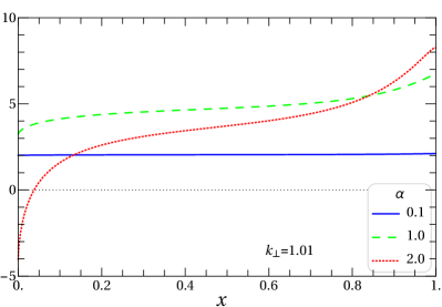
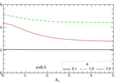
Figure 8: The vertex function $\Gamma_{2}^{(3){j=0}}(k_{\perp},x)$ as a function of $x$ at fixed $k_{\perp}$ (left panel), and as a function of $k_{\perp}$ at fixed $x$ (right panel), calculated in the three-body truncation for several values of the physical coupling constant $\alpha$. The PV mass has been removed by taking the limit $\mu_{1}\to\infty$.

The curves in Fig. 8 reflect typical behavior of $\Gamma_{2}^{(3){j=0}}(k_{\perp},x)$ as a function of its arguments.

Our calculations distinctly indicate that the physical coupling constant $\alpha$ cannot be taken arbitrarily large. If we fix $x$ and consider $\Gamma_{2}^{(3){j=0}}$ as a function of $k_{\perp}$, its limiting ($k_{\perp}\to\infty$) value rapidly increases in magnitude with the increase of $\alpha$. The same happens in the limit $x\to 0$ at fixed $k_{\perp}$. At certain $\alpha=\alpha_{c}$ it seems that $\Gamma_{2}^{(3){j=0}}$ becomes unbounded. Further increase of $\alpha$ leads to the absence of stable numerical solutions of Eq. (LABEL:G2ff). Numerical estimations give $\alpha_{c}\simeq 2.630$. In the next section we will explain the reason why the critical coupling appears in the given physical model and calculate $\alpha_{c}$ exactly.

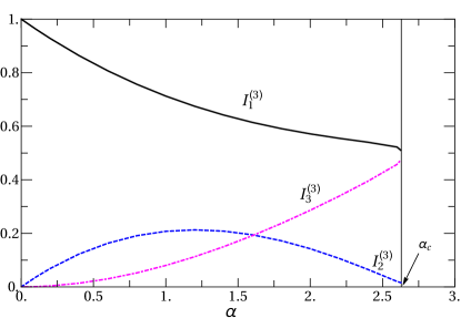
Figure 9: Fock sector norms in the three-body truncation as a function of the physical coupling constant $\alpha$.

To estimate relative contributions of different Fock sectors to the full state vector norm, we calculated the corresponding sector norms as a function of the coupling constant which varies from zero up to the critical value. The results are presented in Fig. 9. One observes that the one-body sector always dominates, though its contribution monotonically decreases with the increase of the coupling constant. The behavior of the two-body sector contribution looks nontrivial: it increases to a maximum and then decreases as a function of the coupling constant. The three-body sector contribution increases monotonically, but it does not reach the value of the one-body sector contribution.

VI.2 Renormalization Parameters

Having found $\Gamma_{2}^{(3)j}(k_{\perp},x)$ and $\psi_{1}^{(3)}$, we can calculate the bare coupling constant ${g_{03}=}g_{03}(x)$ from Eq. (76):

$$g_{03}(x) = {\frac{1}{\sqrt{I_{1}^{(3)}}}\left[\frac{g}{\sqrt{1-g^{2}\bar{I}_{2}^{(2)}}}\right.}$$ (82)

$${-\frac{g^{2}}{8\pi^{2}\left[1-g^{2}\bar{I}_{2}^{(2)}\right]}\sum_{j^{\prime}=0}^{1}(-1)^{j^{\prime}}\int_{0}^{1-x}dx^{\prime}\,x^{\prime}\int_{0}^{\infty}\frac{k^{\prime}_{\perp}dk^{\prime}_{\perp}}{{k^{\prime}}^{2}_{\perp}+\mu_{j^{\prime}}^{2}(1-x^{\prime})+m^{2}x^{{}^{\prime}2}}}$$

$${\left.\times\frac{\Gamma_{2}^{(3)j^{\prime}}(k^{\prime}_{\perp},x^{\prime})}{\sqrt{[{k^{\prime}}^{2}_{\perp}(1-x)+m^{2}{x^{\prime}}^{2}(1+x)-\mu^{2}{x^{\prime}}^{2}+\mu_{j^{\prime}}^{2}(1-x-x^{\prime})]^{2}+4{k^{\prime}}^{2}_{\perp}[m^{2}x^{2}+\mu^{2}(1-x)]{x^{\prime}}^{2}}}\right].}$$

Note that the integrand in Eq. (82) is not singular even without PV regularization and the term with $j^{\prime}=1$ in the sum vanishes in the limit $\mu_{1}\to\infty$. Therefore, $g_{03}(x)$ does not contain divergences. As outlined above, it does explicitly depend on $x$.

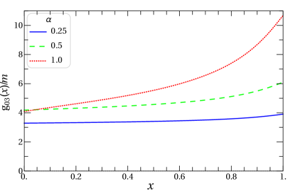
Figure 10: Ratio $g_{03}(x)/m$ as a function of $x$ for a few values of $\alpha$.

In Fig. 10 we show the dependence of $g_{03}$, in units $m$, on the kinematical variable $x$ for several values of the physical coupling constant $\alpha$. If rotational symmetry was not broken by the Fock space truncation, $g_{03}$ would be a true constant independent of $x$. As is seen from Fig. 10, this is not the case: $g_{03}$ depends on $x$; the larger the value of $\alpha$ the stronger is the $x$-dependence. Such a property is a price we pay to have the renormalization condition (75) satisfied for arbitrary $x$. The question of $x$-dependence of $g_{03}$ is discussed below in a special Sec. VIII.

Similarly, the three-body mass counterterm $\delta m_{3}^{2}$ can be found from Eq. (62) in the limit $M\to m$, taking into account the $x$-dependence of $g_{03}$:

$$\delta m_{3}^{2}={-}{\frac{1}{8\pi^{2}\sqrt{I_{1}^{(3)}}}\sum_{j=0}^{1}(-1)^{j}\int_{0}^{1}dx\,g_{03}(x)\int_{0}^{\infty}dk_{\perp}\,k_{\perp}\,\frac{\Gamma_{2}^{(3)j}(k_{\perp},x)}{k^{2}_{\perp}+\mu_{j}^{2}(1-x)+m^{2}x^{2}}}.$$ (83)

In contrast to $g_{03}(x)$, the mass counterterm $\delta m_{3}^{2}$ is a true constant independent of kinematical variables. If $\mu_{1}\to\infty$, $\delta m_{3}^{2}$ diverges like $\log(\mu_{1}/m)$, i.e., one cannot avoid PV particle contributions, when calculating it.

A question may arise, why one should insert $g_{03}(x)$ into the integrand in Eq. (83), rather than to leave it as a free factor [like it appears originally in Eq. (62)], making $\delta m_{3}^{2}$ to be $x$-dependent as well. An answer can not be found in the framework of the three-body Fock space truncation, and the above recipe appears as an ansatz. The rule is however justified in the four-body truncation Li15a ; Li15b , where $g_{03}(x)$ and $\delta m_{3}^{2}$ are necessary to calculate the Fock components. It can be easily seen that $g_{03}(x)$ enters into amplitudes of light-front diagrams constructed according to the FSDR requirements, being integrated over $dx$.

It is instructive to consider not only the mass counterterm $\delta m_{3}^{2}$, but also the three-body self-energy [cf. Eq. (48)]:

$$\Sigma^{(3)}(p^{2})=-\frac{1}{\sqrt{I_{1}^{(3)}}}\sum_{j=0}^{1}(-1)^{j}\int_{0}^{1}\frac{dx\,g_{03}(x)}{2x(1-x)}\int\frac{d^{2}k_{\perp}}{(2\pi)^{3}}\frac{\Gamma_{2}^{(3)j}(k_{\perp},x;p^{2})}{s_{2}^{j}-p^{2}}$$ (84)

with $\delta m^{2}_{3}={\Sigma^{(3)}(m^{2})}$. $\Gamma_{2}^{(3)j}(k_{\perp},x;p^{2})$ is the fully off-energy-shell two-body vertex function, i.e., that introduced in Eq. (28) with $M^{2}=p^{2}\neq m^{2}$. It satisfies the same integral equation (63), changing $M^{2}$ to $p^{2}$, with the renormalization condition $\Gamma_{2}^{(3)j{=0}}(k_{\perp}^{*}(x),x;m^{2})=g\sqrt{I_{1}^{(3)}}$. After simple transformations, fully analogous to those made above, one can derive the following renormalized equation for it:

$$\left[1-\frac{g^{2}\bar{\Sigma}_{r}^{(2)}(\ell_{p}^{2})}{\ell_{p}^{2}-m^{2}}\right]\Gamma_{2}^{(3)j}(k_{\perp},x;p^{2}) = {g\sqrt{1-g^{2}\bar{I}_{2}^{(2)}}}$$ (85)

$$+\frac{g^{2}}{8\pi^{2}}\sum_{j^{\prime}=0}^{1}(-1)^{j^{\prime}}\int_{0}^{1-x}dx^{\prime}\int_{0}^{\infty}dk_{\perp}^{\prime}\,k_{\perp}^{\prime}$$

$$\times\left[V^{jj^{\prime}}(k_{\perp},x,k_{\perp}^{\prime},x^{\prime};p^{2})\Gamma_{2}^{(3)j^{\prime}}(k_{\perp}^{\prime},x^{\prime};p^{2})\right.$$

$$\left.-V^{{0}j^{\prime}}(k_{\perp}^{*}(x),x,k_{\perp}^{\prime},x^{\prime};m^{2})\Gamma_{2}^{(3)j^{\prime}}(k_{\perp}^{\prime},x^{\prime};m^{2})\right],$$

where $\ell_{p}^{2}=-\frac{k_{\perp}^{2}}{x}+p^{2}(1-x)-\mu_{j}^{2}\left(\frac{1-x}{x}\right)$ and

$$V^{jj^{\prime}}(k_{\perp},x,k_{\perp}^{\prime},x^{\prime};p^{2}) = \frac{1}{{k^{\prime}}_{\perp}^{2}+\mu_{j^{\prime}}^{2}(1-x^{\prime})+m^{2}x^{\prime}-p^{2}x^{\prime}(1-x^{\prime})}$$

$$\times\left[(1-x-x^{\prime})^{2}\left(\frac{k_{\perp}^{2}+\mu_{j}^{2}}{x}+\frac{{k^{\prime}}_{\perp}^{2}+\mu_{j^{\prime}}^{2}}{x^{\prime}}+\frac{k_{\perp}^{2}+{k^{\prime}}_{\perp}^{2}+m^{2}}{1-x-x^{\prime}}-p^{2}\right)^{2}-4k_{\perp}^{2}{k^{\prime}}_{\perp}^{2}\right]^{-1/2}.$$

The derivative ${\Sigma^{(3)}}^{\prime}(m^{2})$ is related to the field strength renormalization factor

$$Z^{(3)}_{\chi}=\bigg{[}1{-}{\Sigma^{(3)}}^{\prime}(m^{2})\bigg{]}^{-1}.$$ (87)

In spite of both $\Sigma^{(3)}(p^{2})$ and $\Gamma_{2}^{(3)j}(k_{\perp},x;p^{2})$ having a three-body “origin”, they are actually not needed within the three-body truncation, like $\delta m_{3}^{2}$ and $g_{03}$. So, without going beyond the $N=3$ case, one may ignore the properties of these off-shell quantities. The latter quantities however naturally appear, when finding the Fock components in the four-body truncation, where they affect the calculated results in full measure. In particular, the fully off-energy-shell two-body vertex function $\Gamma_{2}^{(3)j}(k_{\perp},x;p^{2})$ is a source of the critical value of the coupling constant for $N=4$. This point is discussed in more detail in the next section.

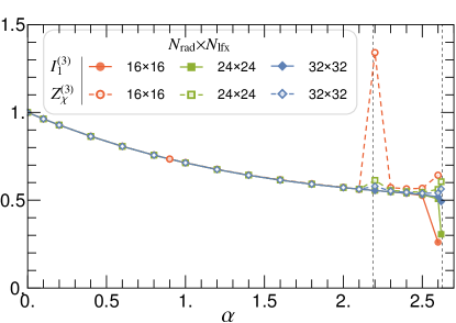
Figure 11: Comparison of the one-body norm $I_{1}^{(3)}$ and the field strength renormalization factor $Z_{\chi}^{(3)}$. $N_{\mbox{\scriptsize rad}}$ and $N_{\mbox{\scriptsize lfx}}$ are, respectively, the numbers of Gaussian integration nodes in the variables $k_{\perp}$ and $x$. $I_{1}^{(3)}$ is obtained from the wave function normalization, Eq. (79). $Z_{\chi}^{(3)}$ is obtained from the self-energy (84) by means of Eq. (87). These two quantities agree within the numerical precision. The dashed lines mark the positions of the critical coupling constants $\alpha_{c}^{{\mbox{\scriptsize nr}}}\simeq 2.190$ (see Sec. VI.3 below) and $\alpha_{{c}}\simeq 2.630$.

The comparison of the calculated value of the field strength renormalization factor $Z^{(3)}_{\chi}$ with the one-body normalization integral $I_{1}^{(3)}$ serves as an additional test of our numerical computations. As is seen from Fig. 11, these two quantities do coincide with each other within the numerical precision.

VI.3 Critical coupling

The parameters entering into the linear integral equation (LABEL:G2ff) — the coupling constant $g$ and the particle masses — should be chosen to allow a physically proper solution for the two-body vertex function. We will not perform here the full analysis, but study the behavior of $\Gamma_{2}^{(3)j}$ as a function of $g$ for fixed values of the particle masses $m$ and $\mu$. Some of our conclusions can be proven analytically, while we will rely on the results of numerical computations for the remainder.

For simplicity, we consider the case of an infinite PV mass $\mu_{1}$. As discussed above, this limit is reached by omitting the term with $j^{\prime}=1$ in the sum in Eq. (LABEL:G2ff). We thus obtain a single linear integral equation for $\Gamma_{2}^{(3)j=0}(k_{\perp},x)$ which we will denote here simply $\Gamma_{2}$, for brevity. Then we represent Eq. (LABEL:G2ff) in the following operator form:

$$\Gamma_{2}=f+\hat{\sf A}\Gamma_{2},$$ (88)

where $f=g\sqrt{1-g^{2}\bar{I}_{2}^{(2)}}$ is the inhomogeneous part, and the operator $\hat{\sf A}$ is represented as a sum of the two contributions

$$\hat{\sf A}=\hat{\sf A}^{\prime}+\hat{\sf K},$$ (89)

where

$$\hat{\sf A}^{\prime}\Gamma_{2} = {\cal F}(\ell^{2})\Gamma_{2}^{(3)j=0}(k_{\perp},x),$$ (90)

$$\hat{\sf K}\Gamma_{2} = \frac{g^{2}}{8\pi^{2}}\int_{0}^{1-x}dx^{\prime}\int_{0}^{\infty}dk_{\perp}^{\prime}\,k_{\perp}^{\prime}\,\Delta V^{00}(k_{\perp},x,k_{\perp}^{\prime},x^{\prime})\Gamma_{2}^{(3)j=0}(k_{\perp}^{\prime},x^{\prime}),$$ (91)

collect, respectively, all nonintegral and integral terms coming from the interaction in the three-body states. The function

$${\cal F}(\ell^{2}){\equiv}\frac{g^{2}\bar{\Sigma}_{r}^{(2)}(\ell^{2})}{\ell^{2}-m^{2}},$$ (92)

where $\ell^{2}$ is given by Eq. (72) with $j=0$, is generated by the scalar nucleon self-energy. The formal solution of Eq. (88), which can be written as $\Gamma_{2}=(1-\hat{\sf A})^{-1}f$, is regular, if the operator $(1-\hat{\sf A})$ is nonsingular. To find out conditions when this is satisfied, we consider a more general eigenvalue problem for the operator $\hat{\sf A}$:

$$\lambda\Gamma_{2}=\hat{\sf A}\Gamma_{2}.$$ (93)

Varying the physical coupling constant, we can trace the behavior of the eigenvalues $\lambda$. As soon as we encounter at least one eigenvalue $\lambda=1$, the solution of Eq. (88) becomes singular.

For numerical analysis, we represent the operator $\hat{\sf A}$ in a matrix form. It can be achieved by discretizing the integrals in Eq. (91) by means of the Gaussian procedure. The same is done for the operator $\hat{\sf A}^{\prime}$ which is reduced to a diagonal matrix. We thus approximate the operator $\hat{\sf A}$ by a finite $n_{A}\times n_{A}$ matrix with the dimension $n_{A}=n_{k}n_{x}$, where $n_{k}$ and $n_{x}$ are the numbers of the integration nodes in the variables $k^{\prime}_{\perp}$ and $x^{\prime}$, respectively. After this transformation, we calculate all the $n_{A}$ eigenvalues $\lambda$. Gradually increasing $n_{A}$, we analyze the spectrum each time till the eigenvalues which are interesting for us become stable.

It is more convenient to work with the dimensionless coupling constant $\alpha$ related to $g^{2}$ by Eq. (4). Evidently, at $\alpha=0$ we have a trivial result $\hat{\sf A}=0$ and the only eigenvalue is $\lambda=0$. Once $\alpha$ starts increasing, the eigenvalues are concentrated in a region of a finite size. We are interested in the maximal real eigenvalue $\lambda_{\mbox{\scriptsize max}}$. Varying $\alpha$, we get a function $\lambda_{\mbox{\scriptsize max}}(\alpha)$. The minimal positive root of the equation $\lambda_{\mbox{\scriptsize max}}(\alpha)=1$ just gives the critical coupling constant $\alpha_{c}$.

The calculated spectrum includes one discrete eigenvalue $\lambda_{0}(\alpha)$ and a set of $(n_{A}-1)$ eigenvalues distributed, almost uniformly, in the interval

$$\lambda_{\mbox{\scriptsize min}}(\alpha)<\lambda<\lambda_{\mbox{\scriptsize max}}(\alpha).$$ (94)

$\lambda_{0}(\alpha)$ is always negative and therefore has no relation to the critical coupling. Note that all the three functions $\lambda_{0}(\alpha)$, $\lambda_{\mbox{\scriptsize min}}(\alpha)$, and $\lambda_{\mbox{\scriptsize max}}(\alpha)$ are very stable as $n_{A}$ increases, while the density of $\lambda$’s between $\lambda_{\mbox{\scriptsize min}}(\alpha)$ and $\lambda_{\mbox{\scriptsize max}}(\alpha)$ grows. This provides a hint that the exact spectrum consists of two parts: a discrete one including the only eigenvalue $\lambda_{0}(\alpha)$ plus a continuous one given by the interval $[\lambda_{\mbox{\scriptsize min}}(\alpha),\,\lambda_{\mbox{\scriptsize max}}(\alpha)]$. The results of the numerical calculation of the spectrum for $m=0.94$ and $\mu=0.14$ are shown in Fig. 12. Note that the functions $\lambda_{0}(\alpha)$, $\lambda_{\mbox{\scriptsize min}}(\alpha)$, and $\lambda_{\mbox{\scriptsize max}}(\alpha)$ are linear, because the operator $\hat{\sf A}$ is proportional to $\alpha$. The relative computational precision is about $10^{-{5}}$, corresponding to $n_{A}\sim 10^{4}$. When $\alpha$ increases, $\lambda_{\mbox{\scriptsize max}}(\alpha)$ reaches unity at $\alpha=\alpha_{c}\simeq 2.630$.

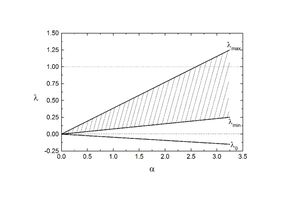
Figure 12: Eigenvalue spectrum of Eq. (93) as a function of the physical coupling constant $\alpha$. The cross-hatched region represents the continuous part of the spectrum, while $\lambda_{0}$ is a discrete eigenvalue.

Our calculation revealed an interesting fact: the continuous part (94) of the spectrum is insensitive to the integral part (91) of the operator $\hat{\sf A}$. In other words, if we calculate the eigenvalue spectrum of $\hat{\sf A}^{\prime}$ by means of the matrix equation

$$\lambda^{\prime}\Gamma_{2}^{\prime}=\hat{\sf A}^{\prime}\Gamma_{2}^{\prime},$$ (95)

then we see that all $n_{A}$ eigenvalues are confined into an interval with the same boundaries $\lambda_{\mbox{\scriptsize min}}(\alpha)$ and $\lambda_{\mbox{\scriptsize max}}(\alpha)$, in spite of the fact that the eigenvectors $\Gamma_{2}$ and $\Gamma_{2}^{\prime}$ are different. The coincidence of the continuous parts of the spectra $\lambda$ and $\lambda^{\prime}$ is not caused by chance but originates from some common property of Eqs. (93) and (95), which will be clear now. The merit of Eq. (95) consists in that it can be trivially solved analytically. Indeed, because of the diagonal form of the matrix $\hat{\sf A}^{\prime}$ the eigenvalues $\lambda^{\prime}$ are simply the values of the function ${\cal F}(\ell^{2})$ at the node points. If $n_{A}\to\infty$, the spectrum becomes continuous:

$$\lambda_{\mbox{\scriptsize min}}(\alpha)<\lambda^{\prime}<\lambda_{\mbox{\scriptsize max}}(\alpha),$$ (96)

where

$$\lambda_{\mbox{\scriptsize min}}(\alpha) = \mbox{min}_{\ell^{2}}{\cal F}(\ell^{2}),$$ (97)

$$\lambda_{\mbox{\scriptsize max}}(\alpha) = \mbox{max}_{\ell^{2}}{\cal F}(\ell^{2}).$$ (98)

It is easy to check that for $0\leq k_{\perp}<\infty$ and $0\leq x\leq 1$ we have $-\infty<\ell^{2}\leq(m-\mu)^{2}$.

The condition (96) has very simple meaning. It means that there always exists such a point $(k_{\perp},x)$ where the solution of the inhomogeneous equation

$$\lambda^{\prime}\Gamma_{2}^{\prime}=f+\hat{\sf A}^{\prime}\Gamma_{2}^{\prime},$$ (99)

which is

$$\Gamma_{2}^{\prime}=\frac{f}{\lambda^{\prime}-{\cal F}(\ell^{2})},$$ (100)

becomes singular. The corresponding equation with the whole operator $\hat{\sf A}$, Eq. (89),

$$\lambda\Gamma_{2}=f+\hat{\sf A}\Gamma_{2},$$ (101)

which is a generalization of our initial equation (88), can not be solved in a similar trivial way, but its formal “solution” can be written

$$\Gamma_{2}=\frac{f+\hat{\sf K}\Gamma_{2}}{\lambda-{\cal F}(\ell^{2})}.$$ (102)

Both expressions on the right-hand sides of Eqs. (100) and (102) have denominators of the same type. Assume we take some value $\lambda$ inside the interval (94) with the boundaries defined by Eqs. (97) and (98). Then the equation ${\cal F}(\ell^{2})=\lambda$ determines a point $\ell^{2}$ [or a set of points $(k_{\perp},x)$] where the denominator in Eq. (102) vanishes. The solution is singular, unless

$$\hat{\sf K}\Gamma_{2}=-f$$ (103)

at the same point. As our analysis shows, this condition is not satisfied. Hence, the stability of the solution of Eq. (LABEL:G2ff) relates to the function ${\cal F}(\ell^{2})$ only. The critical coupling constant is derived from the equation

$$\mbox{max}_{\ell^{2}}{\cal F}(\ell^{2})=1,$$ (104)

where $-\infty<\ell^{2}\leq(m-\mu)^{2}$. To find the maximum, we make use of the explicit form of ${\cal F}(\ell^{2})$:

$${\cal F}(\ell^{2})={-g^{2}{\bar{\Sigma}^{(2)}}{{}^{\prime}}(m^{2})+g^{2}\,\frac{\bar{\Sigma}^{(2)}(\ell^{2})-\bar{\Sigma}^{(2)}(m^{2})}{\ell^{2}-m^{2}}}.$$

Since ${\bar{\Sigma}^{(2)}}{{}^{\prime}}(\ell^{2}){<}0$ [this is distinctly seen, e.g., from Eq. (48)], the difference $\bar{\Sigma}^{(2)}({\ell}^{2})-\bar{\Sigma}^{(2)}({m}^{2})$ is always positive, while the difference ${\ell}^{2}-{m}^{2}$ is negative. So, the quantity $[\bar{\Sigma}^{(2)}({\ell}^{2})-\bar{\Sigma}^{(2)}({m}^{2})]/({\ell}^{2}-{m}^{2})$ is negative. Its maximal (asymptotic) value equals zero, being achieved at $\ell^{2}\to-\infty$. Hence,

$$\mbox{max}_{\ell^{2}}{\cal F}(\ell^{2})={-g^{2}{\bar{\Sigma}^{(2)}}{{}^{\prime}}(m^{2})}$$

and

$$\alpha_{c}=-\left[16\pi m^{2}{{\bar{\Sigma}}^{(2)}}{{}^{\prime}}(m^{2})\right]^{-1}.$$ (105)

Substituting here the explicit form (136) of the derivative of the self-energy, it is easy to see that $\alpha_{c}$ is identical to the critical coupling constant $\alpha_{\textsc{l}}$ associated with the Landau pole (61). For $m=0.94$ and $\mu=0.14$ we obtain $\alpha_{c}\simeq 2.630$, in full agreement with the value found numerically.

Note that $\alpha_{\textsc{l}}$ naturally appears within the two-body approximation, where it nevertheless does not impose any restrictions on the calculated renormalized Fock components. In the three-body case discussed here it appears again but now it substantially affects the behavior of the Fock components. Indeed, for coupling constants above $\alpha_{{c}}$ the equation (LABEL:G2ff) has no physically acceptable solutions. An attempt to calculate the vertex functions numerically for $\alpha>\alpha_{{c}}$ fails: the calculated results oscillate strongly, when the number of integration nodes $n_{A}$ increases, without any tendency to converge. At $\alpha=\alpha_{c}$ the solution of Eq. (LABEL:G2ff) is stable.

We emphasize that the result $\alpha_{c}=\alpha_{\textsc{l}}$ obtained above should be considered as a feature of the Yukawa model rather than a fundamental property of FSDR in the given approximation. The value of the critical coupling constant depends on the particular form of the interaction and can hardly be predicted before analyzing the equations for the Fock components. Indeed, the full eigenvalue spectrum of the equation (93) is determined by the behavior of the self-energy $\bar{\Sigma}^{(2)}$ and the kernel $\Delta V$ as a function of their arguments. In the Yukawa model, the integral part (91) of the operator $\hat{\sf A}$ generates the only eigenvalue $\lambda_{0}(\alpha)$ [in addition to the continuous spectrum governed by the self-energy contribution (90)] having no influence on the stability of the solution. As a result, $\alpha_{c}$ is fully determined by the two-body self-energy, which just makes $\alpha_{c}$ identical to $\alpha_{\textsc{l}}$. For another dynamical model, different from the Yukawa model, the situation may be different.

Going over to a finite PV particle mass does not change the qualitative conclusions, but the numerical value of the critical coupling constant increases. This is not surprising due the fact that each PV subtraction effectively reduces the interaction strength. So, the case $\mu_{1}\to\infty$ analyzed above brings the tightest limitations on admissible values of the coupling constant.

We thus establish that the solution of the renormalized equation (LABEL:G2ff) is nonsingular at $\alpha\leq\alpha_{c}$. This statement however does not concern the initial, nonrenormalized, equation (LABEL:G2f), if the inhomogeneous part $g_{03}\psi_{1}^{(3)}[1-g^{2}\bar{I}_{2}^{(2)}]$ is considered as a free parameter (or an independent function of kinematical variables). Numerical computations show that its solution becomes singular at a lower value of the coupling constant $\alpha=\alpha_{c}^{\mbox{\scriptsize nr}}$, where $\alpha_{c}^{\mbox{\scriptsize nr}}<\alpha_{c}$. The new critical coupling constant now essentially depends on the kernel $V$ of the integral term in Eq. (LABEL:G2f). If we perform the eigenvalue analysis of Eq. (LABEL:G2f) (more precisely, of the corresponding homogeneous equation), we will see the following. The self-energy contribution which is the same as in the renormalized equation (LABEL:G2ff) generates the continuous part of the eigenvalue spectrum (94), as previously, but the discrete eigenvalue $\lambda_{0}(\alpha)$ now is different from that found for the renormalized equation. Moreover, it is positive and always exceeds the upper boundary of the continuous spectrum $\lambda_{\mbox{\scriptsize max}}(\alpha)$, in contrast to the situation shown in Fig. 12. The critical coupling constant $\alpha_{c}^{\mbox{\scriptsize nr}}$ is found as a root of the equation $\lambda_{0}(\alpha_{c}^{\mbox{\scriptsize nr}})=1$. Numerical calculations performed for $m=0.94$, $\mu=0.14$, and an infinite PV mass $\mu_{1}$ give $\alpha_{c}^{\mbox{\scriptsize nr}}\simeq 2.190$. One may conclude that the renormalization removes the singularity of the solution for the two-body vertex function, which appears in the original nonrenormalized equation at $\alpha=\alpha^{\mbox{\scriptsize nr}}_{c}$.

Considering the renormalized equation (85) for the fully off-energy-shell two-body vertex $\Gamma_{2}^{(3)j}(k_{\perp},x;p^{2})$, we encounter a critical coupling constant $\alpha=\alpha_{c}^{\mbox{\scriptsize off}}(p^{2})$, depending on $p^{2}$, which makes $\Gamma_{2}^{(3)j}(k_{\perp},x;p^{2})$ singular. This singularity exists only if $p^{2}\neq m^{2}$. On the mass shell, when we take $p^{2}=m^{2}$, the singularity of $\Gamma_{2}^{(3)j}(k_{\perp},x;m^{2})$ vs. $\alpha$ is absent. Without discussing all technical details, we briefly explain below the origin of $\alpha_{c}^{\mbox{\scriptsize off}}(p^{2})$ and reveal its role in the calculation of Fock components within the FSDR scheme.

Eq. (85) can be solved in two steps. First, we pay attention that setting $p^{2}=m^{2}$ returns us to the renormalized equation (LABEL:G2ff), because $\Gamma_{2}^{(3)j}(k_{\perp},x;m^{2})\equiv\Gamma_{2}^{(3)j}(k_{\perp},x)$. In the second step, on finding the latter function, we can reduce Eq. (85) to

$$\left[1-\frac{g^{2}\bar{\Sigma}_{r}^{(2)}(\ell_{p}^{2})}{\ell_{p}^{2}-m^{2}}\right]\Gamma_{2}^{(3)j}(k_{\perp},x;p^{2}) = G_{0}(x)+\frac{g^{2}}{8\pi^{2}}\sum_{j^{\prime}=0}^{1}(-1)^{j^{\prime}}\int_{0}^{1-x}dx^{\prime}$$ (106)

$$\times\int_{0}^{\infty}dk_{\perp}^{\prime}\,k_{\perp}^{\prime}V^{jj^{\prime}}(k_{\perp},x,k_{\perp}^{\prime},x^{\prime};p^{2})\Gamma_{2}^{(3)j^{\prime}}(k_{\perp}^{\prime},x^{\prime};p^{2}),$$

where the inhomogeneous part given by

$$G_{0}(x)=g\sqrt{1-g^{2}\bar{I}_{2}^{(2)}}-\frac{g^{2}}{8\pi^{2}}\sum_{j^{\prime}=0}^{1}(-1)^{j^{\prime}}\int_{0}^{1-x}dx^{\prime}\int_{0}^{\infty}dk_{\perp}^{\prime}\,k_{\perp}^{\prime}V^{0j^{\prime}}(k_{\perp}^{*}(x),x,k_{\perp}^{\prime},x^{\prime};m^{2})\Gamma_{2}^{(3)j^{\prime}}(k_{\perp}^{\prime},x^{\prime};m^{2})$$ (107)

is already known. As advocated above, the function $\Gamma_{2}^{(3)j}(k_{\perp},x;m^{2})$ is nonsingular at $\alpha\leq\alpha_{c}$. Under this condition, the function $G_{0}(x)$ is also a finite quantity. Eq. (106) now has the same shape as the nonrenormalized equation (LABEL:G2f) for the half-off-shell two-body vertex function $\Gamma_{2}^{(3)j}(k_{\perp},x)$, excepting the fact that the kernel parametrically depends on $p^{2}$. Applying the same eigenvalue analysis, as for Eq. (LABEL:G2f) above, we calculate the critical coupling constants $\alpha^{\mbox{\scriptsize off}}_{c}(p^{2})$. Note that

$$\alpha_{c}^{\mbox{\scriptsize nr}}=\alpha^{\mbox{\scriptsize off}}_{c}(m^{2}).$$ (108)

The right-hand side of Eq. (108) should be understood as a limit $\alpha^{\mbox{\scriptsize off}}_{c}(p^{2}\to m^{2})$, because at $p^{2}=m^{2}$, as has been mentioned above, the two-body vertex function is smooth, even at $\alpha=\alpha_{c}^{\mbox{\scriptsize off}}(m^{2})$. Then, since the critical coupling constant $\alpha_{c}$ defined by Eq. (105) always exists for any of Eqs. (LABEL:G2f), (LABEL:G2ff), and (85), the coupling constant $\alpha_{c}^{\mbox{\scriptsize off}}(p^{2})$ brings new information, only if $\alpha_{c}^{\mbox{\scriptsize off}}(p^{2})<\alpha_{c}$. We emphasize that if $\alpha\leq\alpha_{c}$ and $\alpha\neq\alpha_{c}^{\mbox{\scriptsize off}}(p^{2})$, the solutions of Eqs. (LABEL:G2f), (LABEL:G2ff), and (85) are nonsingular.

The critical coupling constants considered above may generate some peculiarities in $\alpha$-dependence of numerically calculated quantities, especially when using rough computational grids. Indeed, while the exact result is nonsingular, the cancellation of pole contributions may not occur in full measure, due to approximate character of numerical calculations. For instance, sharp behavior of the field strength renormalization factor $Z^{(3)}_{\chi}$ in the vicinity of the point $\alpha=\alpha_{c}^{\mbox{\scriptsize nr}}=2.190$ for a relatively small number of Gaussian integration nodes (see Fig. 11) is a probable manifestation of this effect.

The situation with the simultaneous existence of several types of critical coupling constants looks, at first glance, rather confusing. In order to make it more transparent, in Appendix B we discuss an explicitly solvable toy model which mimics relevant features of the scalar Yukawa model in the three-body truncation. This illustrates our conclusions in a very simple and clear manner.

Within the three-body truncation, all calculated observables are expressed through the renormalized two-body Fock component found for $p^{2}=m^{2}$, while the fully off-shell two-body Fock component $\Gamma_{2}^{(3)j}(k_{\perp},x;p^{2})$ with $p^{2}\neq m^{2}$ is not needed for this purpose. Thus, it may seem that a set of critical constants $\alpha_{c}^{\mbox{\scriptsize off}}(p^{2})$ is a sort of peculiarity having no relation to practical computations of physical quantities, while all actual restrictions imposed on the value of the coupling constant reduces to the requirement $\alpha\leq\alpha_{c}$. The importance of the function $\Gamma_{2}^{(3)j}(k_{\perp},x;p^{2})$ becomes evident as one goes to the four-body truncation, where the former enters, as an internal block, into the system of equations for the Fock components Li15a . In this sense, the fully off-shell two-body vertex function serves as a “bridge” between the three- and four-body truncations. Respectively, the critical coupling constants $\alpha_{c}^{\mbox{\scriptsize off}}(p^{2})$ propagate, together with $\Gamma_{2}^{(3)j}(k_{\perp},x;p^{2})$, to the four-body problem as well. The parameter $p^{2}$ in the four-body truncation varies continuously from $-\infty$ up to $(m-\mu)^{2}$. Our computations for $m=0.94$, $\mu=0.14$, and an infinite PV mass $\mu_{1}$ show that $\alpha_{c}^{\mbox{\scriptsize off}}(p^{2})$ is a decreasing function of $p^{2}$. It reaches its minimal value at the maximal available $p^{2}$, i.e., $p^{2}=(m-\mu)^{2}$. Hence, in the four-body truncation, one may expect the critical coupling constant to be not greater than $\alpha_{c}^{\mbox{\scriptsize off}}((m-\mu)^{2})\simeq 2.382$. At the same time, one cannot exclude the possibility of appearance of a new, purely “four-body”, critical coupling constant. Numerical estimations Li15a ; Li15b based on an iterative procedure show that the iterations stop converging at $\alpha$ about 2.14 or larger. Exact calculation of the critical coupling constant in the four-body truncation however goes beyond the scope of the present paper. The above example with the hierarchy of the critical coupling constants is given to demonstrate that some of them originated from a given order truncation as mathematical peculiarities may then propagate to higher order truncations and then introduce further physical restrictions on the parameters of the model.

VII Calculation of the electromagnetic form factor

Form factors are fundamental for the study of hadron structures. They are defined from the electromagnetic vertex (EMV) $G^{\rho}(p,p^{\prime})$ which is expressed through the matrix element of the current operator $\hat{J}_{\mathrm{em}}^{\rho}(x)$:

$$G^{\rho}(p,p^{\prime})=e_{0}\langle p^{\prime}|\hat{J}^{\rho}_{\mathrm{em}}(0)|p\rangle,$$ (109)

where $p$ and $p^{\prime}$ are the initial and final particle four-momenta, $e_{0}$ is the bare electromagnetic coupling constant, and $\rho$ is an arbitrary Lorentz index. The bra and ket vectors here are the same as the state vectors $\phi^{{\dagger}}(p^{\prime})$ and $\phi(p)$, respectively. The elastic electromagnetic form factor $F(Q^{2})$ for a scalar particle is defined as

$$G^{\rho}(p,p^{\prime})=e(p+p^{\prime})^{\rho}F(Q^{2}),$$ (110)

where $e$ is the physical electromagnetic coupling constant (physical charge), $Q^{2}=-q^{2}$, $q=p^{\prime}-p$ is the four-momentum transfer. The necessity to distinguish the physical and bare electromagnetic coupling constants follows from the fact that the elementary electromagnetic vertex, generally speaking, is renormalized due to its “dressing” by scalar pion lines. The standard renormalization condition known from QED demands that the renormalized EMV at zero momentum transfer must coincide with that for the free particle:

$$G^{\rho}(p,p)=2ep^{\rho}.$$ (111)

This condition yields a relation between $e_{0}$ and $e$.

The structure of the EMV (110) is a consequence of general physical symmetries of the interaction. In approximate nonperturbative calculations in the framework of LFD these symmetries may be broken because of the rotational symmetry violation. This fact may lead to appearance, in the EMV, of nonphysical contributions explicitly depending on the light front orientation Karmanov92 . In the spinless case the problem is however absent for the plus-component of the EMV, provided an additional requirement $q^{+}=0$ is imposed on the momentum transfer. After that, the form factor can be expressed through the EMV by

$$eF(Q^{2})=\frac{G^{+}(p,p^{\prime})}{2p^{+}}.$$ (112)

The renormalization condition (111) is implied to refer to the plus-component of the EMV as well. With Eq. (112), it can be written in a very simple form

$$F(0)=1.$$ (113)

With the Fock representation of the state vector in $N$-body truncated Fock space, the total EMV is a sum of $n$-body contributions ($n=1,\,2,\,\ldots,\,N$) shown in Fig. 13. According to the FSDR rules, the bare electromagnetic coupling constant $e_{0}$ must be a sector-dependent quantity

$$e_{0}\to e_{0l},\quad(l=1,\,2,\ldots,\,N),$$

similar to the bare coupling constant $g_{0}$ which determines the interaction between the constituents of the state vector [see Eq. (29)]. However, in contrast to $g_{0}$ treated nonperturbatively, $e_{0}$ is considered as being small, so that the EMV is calculated in the leading order in $e_{0}$ (at the same time, the renormalization of $e_{0}$ due to its “dressing” by scalar pion lines is nonperturbative!). Then, since $e_{0}$ has no relation to the interactions “inside” the state vector, we will refer to it as an external bare coupling constant Karmanov08 . Now the photon as an external particle should be excluded from the particle counting, and the Fock sector content is fully determined by the number of scalar pion-spectators plus one scalar nucleon. We thus have the following rule to calculate the index $l$ for the $n$-body Fock sector: $l=N-n_{s}$, where $n_{s}=n-1$ is the number of pion-spectators. The lowest order external bare coupling constant $e_{01}=e$, because the trivial case $N=1$ describes the interaction of a photon with a point-like scalar nucleon.

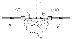
Figure 13: $n$-body electromagnetic vertex in the truncation of order $N$. The dashed line corresponds to a photon. The nucleon-photon interaction vertex is given by $e_{0(N-n+1)}({k}_{1}+{k}_{1}^{\prime})^{\rho}$.

Applying the LFD graph techniques rules to the diagram in Fig. 13 and using Eq. (110), we obtain for the form factor within the $N$-body Fock space truncation:

$$eF^{(N)}(Q^{2})=\sum_{n=1}^{N}e_{0(N-n+1)}F^{(N)}_{n}(Q^{2}),$$ (114)

where

$$F_{n}^{(N)}(Q^{2}) = \frac{2}{(2\pi)^{3(n-1)}(n-1)!}\int\prod_{i=1}^{n}\frac{d^{2}k_{i\perp}dx_{i}}{2x_{i}}$$

$$\times\left[\frac{\Gamma_{n}^{(N)}({\bf k}_{2\perp},x_{2},\ldots,{\bf k}_{n\perp},x_{n})\Gamma_{n}^{(N)}({\bf k}^{\prime}_{2\perp},x_{2},\ldots,{\bf k}^{\prime}_{n\perp},x_{n})}{(s_{n}-m^{2})(s_{n}^{\prime}-m^{2})}\right]\,\delta^{(2)}\left(\sum_{i=1}^{n}{\bf k}_{i\perp}\right)\delta\left(\sum_{i=1}^{n}x_{i}-1\right).$$

The primed transverse momenta are defined as

$${\bf k}^{\prime}_{i\perp}={{\bf k}_{i\perp}-x_{i}{\bf q}_{\perp}},$$

$s^{\prime}_{n}$ is given by Eq. (27), changing ${\bf k}_{i\perp}$ by ${\bf k}^{\prime}_{i\perp}$. Note that, due to the condition $q^{+}=0$, we have $Q^{2}=q_{\perp}^{2}$. Comparison of Eqs. (LABEL:FFn) and (40) gives

$$F_{n}^{(N)}(0)=I_{n}^{(N)},$$ (116)

i.e., the $n$-body contribution to the form factor at zero momentum transfer coincides with the $n$-body Fock sector norm. Setting $Q^{2}=0$ in Eq. (114) and making use of the renormalization condition (113) which writes simply $F^{(N)}(0)=1$ in truncated Fock space, we get

$$e=\sum_{n=1}^{N}e_{0(N-n+1)}I^{(N)}_{n}.$$ (117)

This formula, together with the normalization condition (39) leads to the following result:

$$e_{0l}=e$$ (118)

for arbitrary $l$. So, the electromagnetic coupling constant in the framework of FSDR is not renormalized at all. Eq. (114) now becomes

$$F^{(N)}(Q^{2})=\sum_{n=1}^{N}F^{(N)}_{n}(Q^{2}).$$ (119)

The one-body contribution is

$$F^{(N)}_{1}(Q^{2})=\left[\psi_{1}^{(N)}\right]^{2}=I_{1}^{(N)}=1-\sum_{n=2}^{N}I_{n}^{(N)}.$$ (120)

It does not depend on $Q^{2}$. With Eq. (116), the final expression for the form factor reads

$$F^{(N)}(Q^{2})=1+\sum_{n=2}^{N}\left[F^{(N)}_{n}(Q^{2})-F_{n}^{(N)}(0)\right].$$ (121)

Note that the general formula (LABEL:FFn) for the $n$-body Fock sector contribution to the form factor does not take into account PV particles, since the corresponding integrals do not need regularization in the scalar Yukawa model without antiparticles. One may thus consider Eq. (LABEL:FFn) to be related to the limiting case $\mu_{1}\to\infty$.

In the two-body truncation the form factor is

$$F^{(2)}(Q^{2})=1+F_{2}^{(2)}(Q^{2})-F_{2}^{(2)}(0).$$ (122)

Substituting the solution (51) into Eq. (LABEL:FFn) for $n=N=2$, we arrive at

$$F_{2}^{(2)}(Q^{2})=\frac{g^{2}}{16\pi^{3}}\int_{0}^{1}dx\,x(1-x)\int\frac{d^{2}k_{\perp}}{[k_{\perp}^{2}+\mu^{2}(1-x)+m^{2}x^{2}][({\bf k}_{\perp}-x{\bf q}_{\perp})^{2}+\mu^{2}(1-x)+m^{2}x^{2}]}.$$ (123)

The integrals can be expressed in terms of elementary functions. It is interesting to note that the formulas (122) and (123) exactly reproduce the familiar perturbative result, though our approach does not rely on perturbation theory. This rather surprising fact can be explained by the simplicity of the two-body approximation. Already in the three-body truncation both two- and three-body vertex functions have rather complex dependence on the physical coupling constant, determined by Eqs. (LABEL:G2ff) and (64).

The form factor $F^{(N)}(Q^{2})$ calculated numerically for $N=2$, $N=3$, and $N=4$ is shown in Fig. 14. The calculations were carried out for $m=0.94$, $\mu=0.14$, $\mu_{1}=15$, and two different values of the coupling constant: $\alpha=1.0$ and $\alpha=2.0$. Here we retain a finite PV mass in the two- and three-body truncations in order to compare with the results in the four-body truncation obtained with the same PV mass Li15b . This value of $\mu_{1}$ is large enough to make the calculated results almost insensitive (in the scale of the plots) to its further increase. In principle, in the three-body truncation, one might take a bigger $\alpha$, up to $\alpha_{{c}}{\simeq 2.630}$, inclusive. However, keeping in mind stronger limitations on the coupling constant in the four-body truncation (see the end of Sec. VI.3), we took a lower value of $\alpha$, in order to have the possibility to compare with each other the results for the form factor, obtained in the successive $N=2$, $N=3$, and $N=4$ truncations.

Note that the functions $F_{n}^{(N)}(Q^{2})$, Eq. (LABEL:FFn), with $n\geq 2$ fall rapidly in the asymptotic region $Q^{2}\gg\{m,\,\mu\}$ and tend to zero if $Q^{2}\to\infty$. The limiting value of the form factor thus coincides with the one-body Fock sector norm:

$$F^{(N)}(Q^{2}\to\infty)=I_{1}^{(N)},$$ (124)

that is, generally speaking, a finite nonzero quantity.

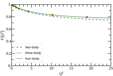
(a)  $\alpha=1.0$

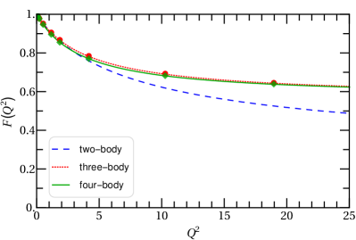
(b)  $\alpha=2.0$

Figure 14: Electromagnetic form factor calculated in the two-, three- and four-body truncations for $\alpha=1.0$ (left panel) and $\alpha=2.0$ (right panel), at $m=0.94$, $\mu=0.14$, and $\mu_{1}=15$. The results for the four-body truncation are adopted from Ref. Li15b . The form factor in the two-body truncation admits an analytic expression. For the three- and four-body truncations, the obtained results (symbols) are fitted to a function (lines) $f(Q^{2})=I_{1}+(1-I_{1})/(1+c_{1}Q^{2})/(1+c_{2}Q^{2})$, where $c_{1}$ and $c_{2}$ are some constants depending on $\alpha$ and on the order of truncation.

VIII Discussion for the $x$-dependence of $g_{03}(x)$

The $x$-dependent bare coupling constant $g_{03}(x)$ was introduced in Ref. Karmanov12 . This $x$-dependence which, at first glance, seems to be an oddity, is a consequence of truncation. As it was already mentioned, by truncating Fock space, we replace the initial light-front Hamiltonian (12) by a finite matrix. Finding, with this finite matrix, the vertex function $\Gamma^{(N)}_{2}(k_{\perp},x)$ and solving the renormalization condition (42) relative to $g_{0N}$, we find that the latter becomes dependent on $x$: $g_{0N}=g_{0N}(x)$ [see Eq. (82) for the $N=3$ case].

More precisely, the mechanism for the appearance of the $x$-dependent $g_{0N}(x)$ is the following. The renormalization condition (42) contains the vertex function $\Gamma^{(N)}_{2}(k_{\perp},x)$ calculated in $N$-body truncated Fock space and dependent on the two kinematical variables $k_{\perp}$ and $x$. The on-energy-shell condition $s_{2}=m^{2}$ does not fix both variables, but gives a relation between them. We express from this relation the value $k_{\perp}=k^{*}_{\perp}(x)$ which is given by Eq. (35). So, the value of the vertex function which appears on the left-hand side of the renormalization condition (42) is $\Gamma^{(N)}_{2}(k^{*}_{\perp}(x),x)$, i.e., it depends on $x$ via $k^{*}_{\perp}(x)$ and also via its “own” argument $x$. Since the right-hand side of Eq. (42) is a constant, this condition can be satisfied identically only if the bare coupling constant $g_{0N}$, which the two-body vertex depends on, becomes a function of $x$ as well.

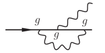
(a)  $\Gamma_{2,a}$

(b)  $\Gamma_{2,b}$

Figure 15: Full set of perturbative contributions to the two-body vertex function at order $\mathrm{O}(g^{3})$. The thinner straight lines represent the scalar nucleon. The thicker straight line represents the antinucleon. The wavy lines represent the scalar pions.

As discussed in Sec. IV, the $x$-dependence of the on-energy-shell two-body vertex function must disappear, if the latter was calculated in full (i.e., not truncated) Fock space. This general property is based on fundamental physical symmetries. To illustrate how the cancellation of $x$-dependence happens in practice, within LFD, there is no need to perform nonperturbative calculations of $\Gamma_{2}^{(N)}(k^{*}_{\perp}(x),x)$ involving contributions from all possible Fock sectors (i.e., for $N\to\infty$). One may use the perturbative expansion of the two-body vertex function, which can be written as

$$\Gamma_{2}^{(N\to\infty)}(k^{*}_{\perp}(x),x)=\sum_{n=1}^{\infty}g^{n}\Gamma_{2}^{(g^{n})}(k^{*}_{\perp}(x),x).$$ (125)

If $\Gamma_{2}^{(N\to\infty)}(k^{*}_{\perp}(x),x)=\mbox{const}$, then any coefficient $\Gamma_{2}^{(g^{n})}(k^{*}_{\perp}(x),x)$ of the perturbation series is also $x$-independent. We emphasize that $\Gamma_{2}^{(g^{n})}$ involves contributions from all possible Fock sectors at order $g^{n}$ of perturbation theory.

The simplest nontrivial case is the third order of perturbation theory. All the contributions to $\Gamma_{2}^{(g^{3})}(k^{*}_{\perp}(x),x)$ are exhausted by the two shown in Fig. 15. The graph (a) generated by the three-body Fock sector (one scalar nucleon plus two scalar pions) represents a contribution incorporated in our nonperturbative three-body calculations of $\Gamma_{2}^{(3)}$ in Sec. VI.1. The graph (b) represents a contribution from another three-body Fock sector (one scalar nucleon plus one nucleon-antinucleon pair), which was omitted in the truncation we used. Below we will demonstrate that the full $\Gamma_{2}^{(g^{3})}(k^{*}_{\perp}(x),x)$, determined by the sum of two contributions (a) and (b), is indeed a constant with respect to $x$.

The amplitude of the diagram in Fig. 15(a) reads

$$\Gamma_{2,a}^{{(g^{3})}}({k}_{\perp},x)=\frac{g^{3}}{(2\pi)^{3}}\int\limits_{0}^{1-x}\frac{dx^{\prime}}{2x^{\prime}(1-x^{\prime})(1-x-x^{\prime})}\int\frac{d^{2}k^{\prime}_{\perp}}{({s_{2}^{\prime}}-m^{2})({s_{3}}-m^{2})}.$$ (126)

The amplitude of the diagram in Fig. 15(b) reads

$$\Gamma_{2,b}^{{(g^{3})}}(k_{\perp},x)=\frac{g^{3}}{(2\pi)^{3}}\int\limits_{1-x}^{1}\frac{dx^{\prime}}{2x^{\prime}(1-x^{\prime})(x+x^{\prime}-1)}\int\frac{d^{2}k^{\prime}_{\perp}}{({s_{2}^{\prime}}-m^{2})({\bar{s}_{3}}-m^{2})}.$$ (127)

The quantities $s_{2}^{\prime}$ and $s_{3}$ defined by Eqs. (34), changing $k_{\perp}\to k^{\prime}_{\perp}$, $x\to x^{\prime}$, and  (65) with $j=j^{\prime}=0$, respectively, are the invariant mass squared of each of the intermediate states of Fig. 15(a): nucleon plus pion and nucleon plus two pions. The quantity $\bar{s}_{3}$ is the invariant mass squared of the three-body state of Fig. 15(b), i.e., the nucleon plus nucleon-antinucleon pair:

$$\bar{s}_{3}=\frac{k^{2}_{\perp}+m^{2}}{1-x}+\frac{{k^{\prime}}^{2}_{\perp}+m^{2}}{1-x^{\prime}}+\frac{({\bf k}_{\perp}+{\bf k}^{\prime}_{\perp})^{2}+m^{2}}{x+x^{\prime}-1}.$$ (128)

Since each of the amplitudes (126) and (127) converge, we omit the PV particle contributions. To calculate the integrals, it is convenient to use the Feynman parametrization:

$$\frac{1}{ab}=\int_{0}^{1}\frac{dv}{[va+(1-v)b]^{2}}.$$

Then both integrals over $d^{2}k^{\prime}_{\perp}$ can be calculated analytically. The integrals over $dv$ are also calculated analytically. We substitute $k_{\perp}=k^{*}_{\perp}(x)$ with the imaginary value $k^{*}_{\perp}{(x)}$ from Eq. (35) and calculate the residual one-dimensional integrals over $dx^{\prime}$ numerically.

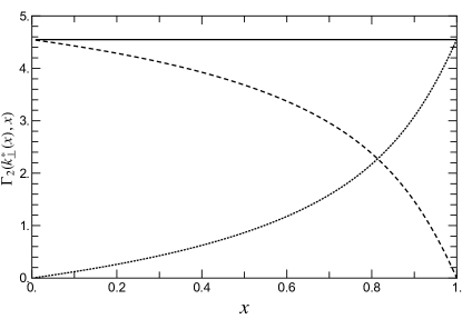
Figure 16: Dependence of the on-energy-shell two-body vertex function in the $g^{3}$-order of perturbation theory on the kinematical variable $x$. The dashed curve is $\Gamma_{2,a}^{{(g^{3})}}(k^{*}_{\perp}(x),x)$, Fig. 15(a); the dotted curve is $\Gamma_{2,b}^{{(g^{3})}}(k^{*}_{\perp}(x),x)$, Fig. 15(b); the solid curve represents their sum which is a constant.

The calculated results are shown in Fig. 16. The dashed curve is $\Gamma_{2,a}^{{(g^{3})}}(k^{*}_{\perp}(x),x)$, the contribution shown in Fig. 15(a). It depends on $x$. This $x$-dependence generates the $x$-dependence of $g_{03}(x)$, Eq. (82). The dotted curve is $\Gamma_{2,b}^{{(g^{3})}}(k^{*}_{\perp}(x),x)$, the contribution shown in Fig. 15(b). It also depends on $x$. The solid line is the sum

$${\Gamma_{2}^{{(g^{3})}}(k^{*}_{\perp}(x),x)}=\Gamma_{2,a}^{{(g^{3})}}(k^{*}_{\perp}(x),x)+\Gamma_{2,b}^{{(g^{3})}}(k^{*}_{\perp}(x),x).$$

It does not depend on $x$. In the Yukawa model with spin, also in the perturbative framework, the same result was found in Ref. Karmanov12 .

This example clearly shows that the origin of the $x$-dependence of the bare coupling constant $g_{03}(x)$ is the Fock space truncation. Taking into account the previously omitted contribution with an antinucleon we restore the constant value of $g_{03}$.

In principle, antiparticle degrees of freedom can be included into Fock space within the nonperturbative approach based on FSDR. This was done in Refs. Mathiot11 (within the scalar Yukawa model) and Karmanov12 (within the spinor Yukawa model in the quenched approximation, i.e., neglecting fermion-antifermion loop contributions). The results of numerical nonperturbative calculations of the on-energy-shell two-body vertex function $\Gamma_{2}^{(3)}(k^{*}_{\perp}(x),x)$ or the bare coupling constant $g_{03}(x)$ in the three-body truncation with the nucleon-nucleon-antinucleon Fock sector included show that the latter makes the $x$-dependence of the calculated quantities much weaker, even for rather large coupling constant values.

IX Conclusion

With the interaction Hamiltonian $\mathcal{H}_{\text{int}}{(x)}=-g\,\chi^{\dagger}\chi\varphi$, where $\chi$ and $\varphi$ are spinless fields referred as a “scalar nucleon” and “scalar pion”, respectively, in the framework of light-front dynamics, we found nonperturbatively the Fock components of the state vector in truncated Fock space including one-body ($\chi$), two-body ($\chi$+$\varphi$), and three-body ($\chi$ +$2\varphi$) states (Fock sectors). The sector dependent renormalization of the coupling constant and the scalar nucleon mass was used. In this transparent example, we exposed the general principles of nonperturbative renormalization in truncated Fock space and demonstrated, by practical application, the main steps required to solve the problem. The procedure contains the principal ingredients of more general applications, and, especially, the main features of the sector dependent renormalization – appearance of the sector dependent renormalization parameters, i.e., the bare coupling constants like $g_{02}$, $g_{03}$ and the mass counterterms like $\delta m^{2}_{2}$, $\delta m_{3}^{2}$, related to different Fock sectors, simultaneously in one system of equations for the Fock components. Though the constant $g_{03}$ is not a true constant – it depends on the kinematical variable $x$, – this and other constants do not contain any uncertainties and are found unambiguously.

The case of the true Yukawa model (or other field theories), incorporating spin, differs from the example considered here by technical details only (the form of propagators, the spin structure of the wave functions, etc.), but contains the same steps. The case of higher order truncation is more complicated technically, since it requires the solution of a more complicated system of equations, but it uses the same solution procedure.

This work presents the detailed theoretical framework that underlines the successful solution of the scalar Yukawa model in four-body truncation when the ($\chi$+$3\varphi$) Fock sector is added to the three listed above Li15a ; Li15b . Comparison of results in the three-body truncation with those in four-body truncation Li15a ; Li15b shows that convergence with respect to the number of Fock sectors involved is achieved.

Appendix A Two-body self-energy

The two-body scalar nucleon self-energy is given by Eq. (48) which can be written as

$$\bar{\Sigma}^{(2)}(p^{2})={-}\frac{1}{16\pi^{2}}\sum_{j=0}^{1}(-1)^{j}\int_{0}^{1}dx\int_{0}^{\infty}\frac{dk_{\perp}^{2}}{k_{\perp}^{2}+\mu_{j}^{2}(1-x)+m^{2}x-p^{2}x(1-x)}.$$ (129)

Without PV regularization, the integral over $dk_{\perp}^{2}$ diverges logarithmically at the upper limit. It is convenient to define the regular function

$$a(p^{2},m_{1},m_{2})\equiv\int_{0}^{1}dx\int_{0}^{\infty}dk_{\perp}^{2}\,\left[\frac{1}{k_{\perp}^{2}+m_{1}^{2}(1-x)+m_{2}^{2}x-p^{2}x(1-x)}-\frac{1}{k_{\perp}^{2}+m^{2}}\right].$$ (130)

Then

$$\bar{\Sigma}^{(2)}(p^{2})={-}\frac{1}{16\pi^{2}}\left[a(p^{2},\mu,m)-a(p^{2},\mu_{1},m)\right].$$ (131)

The integrals in Eq. (130) are easily calculated. We introduce the notation

$$D\equiv p^{4}-2(m_{1}^{2}+m_{2}^{2})p^{2}+(m_{1}^{2}-m_{2}^{2})^{2}.$$

Then

$$a(p^{2},m_{1},m_{2})=2-\log\frac{m_{1}m_{2}}{m^{2}}+\frac{m_{1}^{2}-m_{2}^{2}}{p^{2}}\log\frac{m_{2}}{m_{1}}+\frac{\sqrt{|D|}}{p^{2}}\,\Phi(p^{2},m_{1},m_{2}),$$ (132)

where

$$\Phi(p^{2},m_{1},m_{2})=\left\{\begin{array}[]{lll}\log\left(\frac{m_{1}^{2}+m_{2}^{2}-p^{2}+\sqrt{D}}{2m_{1}m_{2}}\right),&\mbox{if}&D\geq 0,\\ -\arctan\left(\frac{\sqrt{|D|}}{m_{1}^{2}+m_{2}^{2}-p^{2}}\right),&\mbox{if}&D<0.\end{array}\right.$$ (133)

The function $a(p^{2},m_{1},m_{2})$ is symmetric with respect to the permutation of $m_{1}$ and $m_{2}$. At $p^{2}<(m_{1}+m_{2})^{2}$ it is real.

In the limit of infinite PV mass $\mu_{1}$ the difference $\bar{\Sigma}^{(2)}_{c}(p^{2})=\bar{\Sigma}^{(2)}(p^{2})-\bar{\Sigma}^{(2)}(m^{2})$ tends to a finite value:

$$\bar{\Sigma}^{(2)}_{c}(p^{2})={-}\frac{1}{16\pi^{2}}\left[a(p^{2},\mu,m)-a(m^{2},\mu,m)\right].$$ (134)

At $p^{2}\to-\infty$ we get the following asymptotic behavior:

$$\bar{\Sigma}^{(2)}_{c}(p^{2})\approx{\frac{1}{16\pi^{2}}\log\frac{|p^{2}|}{m^{2}}}+\ldots,$$ (135)

where the dots designate finite terms.

In contrast to the self-energy, its derivative over $p^{2}$ does not need regularization, so, ${\bar{\Sigma}^{(2)}}{{}^{\prime}}(m^{2})$ is finite in the limit of infinite PV mass. Its limiting value is calculated as

$${\bar{\Sigma}^{(2)}}{{}^{\prime}}(m^{2})={-}\frac{1}{16\pi^{2}}\,\left.\frac{\partial a(p^{2},\mu,m)}{\partial p^{2}}\right|_{p^{2}=m^{2}}.$$

The calculation of the derivative is straightforward. It yields

$${\bar{\Sigma}^{(2)}}{{}^{\prime}}(m^{2})={-}\frac{1}{16\pi^{2}m^{2}}\left[\frac{\xi(3-\xi^{2})}{\sqrt{4-\xi^{2}}}\,\arctan\left(\frac{\sqrt{4-\xi^{2}}}{\xi}\right)-1+(1-\xi^{2})\log\frac{1}{\xi}\right],$$ (136)

where $\xi=\mu/m$. Eq. (136) is valid for $\mu<2m$.

Appendix B Critical coupling constant in explicitly solvable model

In this section we consider, as an illustration, an explicitly solvable model which reflects all important properties of Eqs. (LABEL:G2f), (LABEL:G2ff), and (85), related to the existence of the critical coupling constant. We will not analyze the “Landau pole” type critical coupling constant (60) caused by the two-body self-energy contribution but, instead, focus on the critical coupling originating from the kernel of the integral term in each of the equations discussed. According to the terminology of Sec. VI.3, we are interested in the critical coupling constant coming from the discrete eigenvalue $\lambda_{0}$ which strongly depends on the particular form of the integration kernel.

Each of the equations is a Fredholm integral equation of the second kind, which can be written schematically in the form (88). The integral operator $\hat{\sf A}$ depends on the coupling constant $\alpha$. The critical coupling constant $\alpha_{c}$ is a solution of the matrix equation $\det(\hat{\sf A}-{\sf I})=0$, where ${\sf I}$ is a unity matrix. If $\alpha=\alpha_{c}$, the solution $\Gamma_{2}$ as a function of $\alpha$ becomes singular: it has a pole $\sim 1/(\alpha-\alpha_{c})$.

Let us first summarize what is already known about, concerning the critical coupling in the equations mentioned above. The equation (LABEL:G2f) for the nonrenormalized $\Gamma_{2}^{(3)j}(k_{\perp},x)$, where the inhomogeneous part $g_{03}\psi_{1}^{(3)}[1-g^{2}\bar{I}_{2}^{(2)}]$ is treated as an independent quantity (a constant or a function of $x$), has a critical coupling constant. For the physical particle masses $m=0.94$, $\mu=0.14$, and an infinite PV mass $\mu_{1}$ its value is $\alpha_{c}^{\mbox{\scriptsize nr}}\simeq 2.190$. After the renormalization leading to Eq. (LABEL:G2ff), this critical coupling disappears, i.e., the renormalized $\Gamma_{2}^{(3)j}(k_{\perp},x)$ is smooth at $\alpha=\alpha_{c}^{\mbox{\scriptsize nr}}$. We see that the role of renormalization in deleting infinities is two-fold: the renormalization not only deletes field theoretical divergences (e.g., the logarithmic ultraviolet divergence in the two-body self-energy $\Sigma^{(2)}$), but also removes the pole singularity of the Fock components at $\alpha=\alpha_{c}^{\mbox{\scriptsize nr}}$. In the generalized equation (85) for the fully off-shell two-body vertex function $\Gamma_{2}^{(3)j}(k_{\perp},x;p^{2})$ the critical coupling constant arises again, now as a function of $p^{2}$. We will show that all these properties can be easily traced and explained by using a toy model which admits analytic solution.

We start with the equation

$$F(k,x)=g_{0}(x)\psi_{1}+\int K(k,x,k^{\prime},x^{\prime})F(k^{\prime},x^{\prime})dk^{\prime}dx^{\prime}$$ (137)

with the separable kernel

$$K(k,x,k^{\prime},x^{\prime})=\alpha h(k,x)h(k^{\prime},x^{\prime}).$$ (138)

Here $F$ is an unknown function to be found, $g_{0}$ and $h$ are smooth bounded functions of their arguments, and $\psi_{1}$ is a constant. We do not specify the limits of integration, assuming that all integrals hereafter are convergent (e.g., due to proper regularization). Eq. (137) is an analog of the equation (LABEL:G2f) for the nonrenormalized two-body vertex function. Its solution is easily found and has the form

$$F(k,x)=g_{0}(x)\psi_{1}+\frac{\alpha h(k,x)}{1-\frac{\alpha}{\alpha_{c}}}\int h(k^{\prime},x^{\prime})g_{0}(x^{\prime})\psi_{1}dk^{\prime}dx^{\prime},$$ (139)

where

$$\frac{1}{\alpha_{c}}=\int h^{2}(k^{\prime},x^{\prime})dk^{\prime}dx^{\prime}.$$ (140)

It is seen that $F(k,x)$ is singular at $\alpha=\alpha_{c}$. The latter quantity is a full analog of the critical coupling constant $\alpha_{c}^{\mbox{\scriptsize nr}}$ (see Sec. VI.3).

Now we apply a “renormalization” procedure to the function $F(k,x)$. In the Yukawa model we imposed the renormalization condition on the function $\Gamma_{2}^{(N)}(k_{\perp},x)$ at $s_{{2}}=m^{2}$ which corresponds to an $x$-dependent point $k_{\perp}=k^{*}_{\perp}(x)$ given by Eq. (35). We will keep this analogy and impose the renormalization condition on $F(k,x)$ in some point $k=k^{*}(x)$:

$$F(k^{*}(x),x)=g$$ (141)

and demand its fulfillment for all values of $x$. Now the function $g_{0}(x)$ can not be considered as being fixed a priori and should be found along with the renormalized $F(k,x)$. Substituting $F(k,x)$ from Eq. (139) into Eq. (141), we get

$$g_{0}(x)\psi_{1}+\frac{\alpha h(k^{*}(x),x)}{1-\frac{\alpha}{\alpha_{c}}}\int h(k^{\prime},x^{\prime})g_{0}(x^{\prime})\psi_{1}dk^{\prime}dx^{\prime}=g.$$ (142)

This equation is easily solved relative to $g_{0}(x)$. After that, we find the relation between the “bare” ($x$-dependent) coupling constant $g_{0}(x)$ and the “physical” one, $g$:

$$g_{0}(x)\psi_{1}=g\left(\frac{1-\frac{\alpha}{\alpha_{c}}+\alpha\int\bigl{[}h(k^{*}(x^{\prime}),x^{\prime})-h(k^{*}(x),x)\bigr{]}h(k^{\prime},x^{\prime})dk^{\prime}dx^{\prime}}{1-\frac{\alpha}{\alpha_{c}}+\alpha\int h(k^{*}(x^{\prime}),x^{\prime})h(k^{\prime},x^{\prime})dk^{\prime}dx^{\prime}}\right).$$ (143)

Substituting this expression for $g_{0}(x)\psi_{1}$ into Eq. (139), we obtain the renormalized solution

$$F(k,x)=g+\frac{g\alpha[h(k,x)-h(k^{*}(x),x)]\int h(k^{\prime},x^{\prime})dk^{\prime}dx^{\prime}}{1-\frac{\alpha}{\alpha_{c}}+\alpha\int h(k^{*}(x^{\prime}),x^{\prime})h(k^{\prime},x^{\prime})dk^{\prime}dx^{\prime}}.$$ (144)

It satisfies the equation

$$F(k,x)=g+\int\left[K(k,x,k^{\prime},x^{\prime})-K(k^{*}(x),x,k^{\prime},x^{\prime})\right]F(k^{\prime},x^{\prime})dk^{\prime}dx^{\prime}$$ (145)

analogous to the equation (LABEL:G2ff) for the renormalized two-body vertex function. Note that after the renormalization $F(k,x)$ has no any singularity at $\alpha=\alpha_{c}$.

The mechanism for the removal of the singularity at $\alpha=\alpha_{c}$ is nontrivial, since it is not reduced to the cancellation of factors like $(\alpha-\alpha_{c})$. Such a cancellation would take place if $g_{0}(x)$ did not depend on $x$. To explain this point, consider, for a moment, another form of the renormalization condition, as compared to Eq. (141). Namely, we impose it not for all values of $x$ simultaneously, but for a particular value $x=x^{*}$ only: $F(k^{*}(x^{*}),x^{*})=g$. Now, expressing the product $g_{0}\psi_{1}$ via $\alpha$, we obtain that the former is a true constant proportional to $(\alpha-\alpha_{c})$. It cancels the $1/(\alpha-\alpha_{c})$ singularity of the nonrenormalized solution. At $\alpha=\alpha_{c}$ the inhomogeneous term vanishes and the renormalized $F(k,x)$ becomes a solution of the homogeneous equation, which exists just at this critical value of $\alpha$. After the $x$-dependence of $g_{0}(x)$ is taken into account (as it should be), the function $g_{0}(x)$ does not turn into zero at $\alpha=\alpha_{c}$, in contrast to the case $g_{0}(x)=const$. The cancellation of the singularity $1/(\alpha-\alpha_{c})$ in Eq. (139) takes place only after the calculation of the double integral. Due to this fact the renormalized solution becomes nonsingular and smooth at $\alpha=\alpha_{c}$.

It is also instructive to find the corresponding “off-shell” solution satisfying the equation [cf. with Eq. (137)]:

$$F(k,x;p)=g_{0}(x)\psi_{1}(p)+\int K(k,x,k^{\prime},x^{\prime};p)F(k^{\prime},x^{\prime};p)dk^{\prime}dx^{\prime},$$ (146)

where

$$K(k,x,k^{\prime},x^{\prime};p)=\alpha h(k,x;p)h(k^{\prime},x^{\prime};p).$$ (147)

The “off-shell” continuation is given by the additional dependence of all parts of the equation on the parameter $p$. The “on-shell” equation, completely equivalent to Eq. (137), is obtained at $p=m$. The renormalization condition is still imposed on the mass shell $p=m$:

$$F(k^{*}(x),x;m)=g,$$

whereas Eq. (146) determines the solution $F(k,x;p)$ for arbitrary $p$. After the renormalization, Eq. (146) becomes an analog of Eq. (85). Its solution can be found in a similar fashion to the on-shell solution (144) and has the form

$$F(k,x;p) = g\frac{\psi_{1}(p)}{\psi_{1}(m)}\left\{1-\alpha\frac{J_{1}(m)h(k^{*}(x),x;m)}{1-\frac{\alpha}{\alpha_{c}(m)}+\alpha J_{2}(m)}+\alpha\left[\frac{1-\frac{\alpha}{\alpha_{c}(m)}}{1-\frac{\alpha}{\alpha_{c}(p)}}\right]\frac{J_{1}(p)h(k,x;m)}{1-\frac{\alpha}{\alpha_{c}(m)}+\alpha J_{2}(m)}\right.$$ (148)

$$+ \left.\alpha\left[\frac{J_{1}(p)J_{2}(m)-J_{1}(m)J_{2}(p)}{1-\frac{\alpha}{\alpha_{c}(p)}}\right]\frac{h(k,x;p)}{1-\frac{\alpha}{\alpha_{c}(m)}+\alpha J_{2}(m)}\right\},$$

where

$$J_{1}(p) = \int h(k^{\prime},x^{\prime};p)dk^{\prime}dx^{\prime},$$

$$J_{2}(p) = \int h(k^{\prime},x^{\prime};p)h(k^{*}(x^{\prime}),x^{\prime};m)dk^{\prime}dx^{\prime},$$

and

$$\frac{1}{\alpha_{c}(p)}=\int h^{2}(k^{\prime},x^{\prime};p)dk^{\prime}dx^{\prime}.$$

A peculiarity of the solution (148) consists in the fact that, in contrast to the on-shell renormalized solution (144), it is singular at $\alpha=\alpha_{c}(p)$, in spite of renormalization. A similar peculiarity happens with the fully off-shell two-body vertex function $\Gamma_{2}^{(3)j}(k_{\perp},x;p^{2})$ which is singular at $\alpha=\alpha_{c}^{\mbox{\scriptsize off}}(p^{2})$.

On the mass shell $p=m$, we find that

$$\left[\frac{1-\frac{\alpha}{\alpha_{c}(m)}}{1-\frac{\alpha}{\alpha_{c}(p)}}\right]_{p=m}\Rightarrow 1,$$

$$\left[\frac{{J}_{1}(p){J}_{2}(m)-{J}_{1}(m){J}_{2}(p)}{1-\frac{\alpha}{\alpha_{c}(p)}}\right]_{p=m}\Rightarrow 0.$$

Then the solution (148) coincides with the on-shell solution (144) and it is nonsingular at $\alpha=\alpha_{c}(m)$.

It is interesting to trace how the singularity at $\alpha=\alpha_{c}(p)$ disappears, when $p\to m$. Extracting the pole term $\sim[\alpha-\alpha_{c}(p)]^{-1}$ from Eq. (148) in this limit, we get, up to terms of order $(p-m)$, inclusive:

$$F(k,x;p\to m)=c\cdot\frac{h(k,x;m)(p-m)}{\alpha-\alpha_{c}(p)}+\ldots,$$ (149)

where

$$c=\frac{g\left\{\alpha_{c}(m)[J_{1}(m)J_{2}^{\prime}(m)-J_{1}^{\prime}(m)J_{2}(m)]+\alpha_{c}^{\prime}(m)J_{1}(m)\right\}}{J_{2}(m)},$$

the primes denote the corresponding derivatives and the dots designate all nonpole contributions. At $\alpha=\alpha_{c}(p)$ the solution (149) vs. $\alpha$ is singular for arbitrary $p\neq m$, though the residue at the pole reduces when $p$ approaches $m$. The singularity disappears only if $p$ exactly equals $m$. So, the cancellation of the singularity in the on-shell solution $F(k,x;m)$ happens due to subtle balance between different terms in the equation, caused by the renormalization.

The above analysis distinctly shows that there exists one-to-one correspondence between the properties of this toy model and the scalar Yukawa model, concerning the behavior of their solutions as a function of the coupling constant. Thus, in each of the two models
(i) the nonrenormalized solution has a pole at a certain (critical) value of the coupling constant $\alpha=\alpha_{c}$;
(ii) the singularity $1/(\alpha-\alpha_{c})$ disappears after the renormalization and the renormalized solution is smooth at $\alpha=\alpha_{c}$;
(iii) both the “off-shell” solution like the two-body vertex $\Gamma_{2}^{(3)j}(k_{\perp},x;p^{2})$ introduced in Sec. VI.2 and the function $F(k,x;p)$ satisfying Eq. (146) are singular at some (critical) value of the coupling constant $\alpha=\alpha_{c}(p)$ depending on the parameter $p$, even after renormalization;
(iv) the pole $1/[\alpha-\alpha_{c}(p)]$ of the “off-shell” solution exists for an arbitrary value of $p$, not equal to its on-mass-shell value $m$, and disappears identically for $p=m$ only.

References

- (1) R.J. Perry, A. Harindranath, and K.G. Wilson, Phys. Rev. Lett. 65, 2959 (1990).
- (2) P.A.M. Dirac, Rev. Mod. Phys. 21, 392 (1949).
- (3) J. Carbonell, B. Desplanques, V.A. Karmanov, and J.-F. Mathiot, Phys. Rep. 300, 215 (1998).
- (4) S.J. Brodsky, H. Pauli, and S.S. Pinsky, Phys. Rep. 301, 299, (1998).
- (5) F. Coester, Prog. Part. Nucl. Phys. 29, 1 (1992).
- (6) V.A. Karmanov, J.-F Mathiot, and A.V. Smirnov, Phys. Rev. D 77, 085028 (2008).
- (7) V.A. Karmanov, J.-F. Mathiot, and A.V. Smirnov, Phys. Rev. D 86, 085006 (2012).
- (8) Y. Li, V.A. Karmanov, P. Maris, and J.P. Vary, Few-Body Syst. 56, 495 (2015).
- (9) Y. Li, V.A. Karmanov, P. Maris, and J.P. Vary, Phys. Lett. B 748, 278 (2015).
- (10) D. Bernard, Th. Cousin, V.A. Karmanov, and J.-F. Mathiot, Phys. Rev. D 65, 025016 (2001).
- (11) J.R. Hiller and S.J. Brodsky, Phys. Rev. D 59, 016006 (1998).
- (12) G. Baym, Phys. Rev. 117, 886 (1960).
- (13) F. Gross, Ç. Şavkli, and J. Tjon, Phys. Rev. D 64, 076008, (2001).
- (14) V.A. Karmanov, J.-F Mathiot, and A.V. Smirnov, Phys. Rev. D 69, 045009 (2004)
- (15) M. E. Peskin and D. V. Schroeder, An Introduction To Quantum Field Theory, Addison-Wesley Advanced Book Program, 1995.
- (16) V.A. Karmanov, J.-F. Mathiot, and A.V. Smirnov, Phys. Rev. D 82, 056010 (2010).
- (17) J.-F. Mathiot, A.V. Smirnov, N.A. Tsirova, and V.A. Karmanov, Few-Body Syst. 49, 183 (2011).
- (18) V.A. Karmanov and A.V. Smirnov, Nucl. Phys. A546, 691 (1992).