Abstract

We construct a monotone version of an empirical Bayes estimator for the parameter of the Borel-Tanner distribution. Some properties of the estimator’s regret risk are illustrated through simulations.

1 Introduction

The probability mass function (p.m.f.) of Borel-Tanner (BT) distribution is

$$p_{r}(x;\theta)=c_{r}(x)\theta^{x-r}e^{-\theta x}\qquad x=r,r+1,\ldots,$$ (1)

where $0<\theta<1$, $r$ is a positive integer, and $c_{r}(x):=rx^{x-r-1}/(x-r)!$

The BT distribution arises, for example, branching processes models and queueing theory. Originally (1) was derived as the distribution of the number of customers served in a busy period of a single-server queuing process, started with $r$ customers and having traffic intensity $\theta$, assuming Poisson arrivals and constant service time. Later BT distribution appeared in the theory of branching processes. If the number of offspring that an individual has is Poisson-distributed with offspring mean $0<\theta<1$, then the total progeny of a Galton-Watson process starting with $r$ ancestors is a random variable with p.m.f. (1). More recently, the distribution has been used to model a variety of real-world phenomena including: coalescence models (Aldous (1999)), highway traffic flows (Koorey (2007)), propagation of internet viruses (Sellke et al. (2005)), cascading failures of energy systems (Ren et al. (2013)) and herd size in finance modeling (Nirey et al. (2012)). Our interest in estimating $\theta$ stems from its role as the reproduction number of an epidemic infection modeled by a branching process (Farrington et al. (2003)).

In the context of branching processes, the parametric Bayesian statistical approach was first explored by Dion (1972) and Jagers (1975), Section 2.13 (see also Guttorp (1991), Chapter 4). Adopting the Bayesian framework, suppose $\theta\in\Omega$ is a realization of a random variable $\Theta$, having a prior distribution $G$. It is well-known that, under the squared error loss, the value $\theta_{G}(x)$ of the Bayesian estimator for $\theta$ is the posterior mean

$$\theta_{G}(x)=E\left[\Theta\ |\ X=x\right]=\frac{\displaystyle\int_{\Omega}\theta^{x+1-r}e^{-x\theta}dG(\theta)}{\displaystyle\int_{\Omega}\theta^{x-r}e^{-x\theta}dG(\theta)}.$$ (2)

Example 1 Let the prior $G$ be Beta$(v,w)$, $v,w>0$. One can verify (see Moll (2015), p.97 for the evaluation of the integrals) that (2) yields

$$\theta_{G}(x)=\frac{\displaystyle\sum_{k=0}^{w-1}(-1)^{k}{w-1\choose k}\frac{\displaystyle(x-r+v+k)!}{x^{k+1}}\left[e^{x}-Exp_{x-r+v+k}(x)\right]}{\displaystyle\sum_{k=0}^{w-1}(-1)^{k}{w-1\choose k}\frac{\displaystyle(x-r+v+k-1)!}{x^{k}}\left[e^{x}-Exp_{x-r+v+k-1}(x)\right]},$$ (3)

where $Exp_{j}(x):=\sum_{k=0}^{j}x^{k}/k!$.

Example 2 If the prior $G$ is Uniform$(0,1)$, then (3) simplifies to

$$\theta_{G}(x)=\frac{x+1-r}{x}\ \frac{\displaystyle e^{x}-Exp_{x+1-r}(x)}{\displaystyle e^{x}-Exp_{x-r}(x)}.$$ (4)

We shall adopt the empirical Bayes (EB) approach, which relies on the assumption for existence of a prior $G$ which, however, is unknown. Suppose our estimation problem is one in a sequence of similar problems with the same prior distribution. In this scenario, the results of previous studies can be used to estimate the prior $G$ and/or the Bayes rule $\theta_{G}$ directly. More precisely, consider a sequence of independent copies

$$(X_{1},\Theta_{1}),(X_{2},\Theta_{2}),\ldots,(X_{n},\Theta_{n}),\ldots$$

of the random pair $(X,\Theta)$, where $\Theta$ has a distribution $G$, and conditional on $\Theta$, $X$ has the BT distribution (1). Assume that $X_{i}$, $i=1,2,\ldots$ are observable, but $\Theta_{i}$, $i=1,2,\ldots$ are not observable. We let $X_{n+1}$ stand for the present random observation, and $\underline{X}(n):=(X_{1},\ldots,X_{n})$ denote the $n$ past observations. Let $\theta_{n+1}$ be the present parameter value of the variable $\Theta$. An EB estimator $\theta_{n}(X_{n+1},\underline{X}(n))=:\theta_{n}(X)$ for the parameter $\theta$ is a function of the currently observed $X_{n+1}$ and the past data $\underline{X}(n)$. In general, it is difficult to find an estimator $\theta_{n}(X)$ for $\theta$ by estimating the Bayes rule $\theta_{G}$ directly. In case of BT distribution, Liang (2009) succeeded in constructing such EB estimator $\theta_{n}(X)$ for $\theta_{G}$ as follows. For $x=r,r+1,\ldots$ let

$$\psi_{n}(x):=\frac{1}{n}\sum_{j=1}^{n}\frac{c_{1}(X_{j}-x)I\{X_{j}\geq x+1\}}{c_{r}(X_{j})}\quad\mbox{and}\quad q_{n}(x):=\frac{1}{n}\sum_{j=1}^{n}\frac{I\{X_{j}=x\}}{c_{r}(x)}.$$

Define an EB estimator $\theta_{n}(X)$ for each $x=r,r+1,\ldots$ by

$$\theta_{n}(x):=\min\left\{\frac{\psi_{n}(x)}{q_{n}(x)},1\right\},\qquad q_{n}(x)\neq 0.$$ (5)

By definition, the Bayesian estimator $\theta_{G}(X)$ minimizes the Bayes risk defined (for the squared error loss function) as

$$R(G,\theta_{G}):=E_{(X,\Theta)}[\Theta-\theta_{G}(X)]^{2}.$$

The Bayes risk of the EB estimator $\theta_{n}(X)$ is

$$R(G,\theta_{n}):=E_{n}E_{(X_{n+1},\Theta_{n+1})}[\Theta_{n+1}-\theta_{n}(X_{n+1})]^{2}.$$

The difference

$$S(\theta_{n}):=R(G,\theta_{n})-R(G,\theta_{G})\geq 0$$

is called the regret risk of $\theta_{n}$ and measures the quality of $\theta_{n}$. In particular, $\theta_{n}$ is asymptotically optimal for $G$ if $\lim_{n\to\infty}S(\theta_{n})=0$. Liang (2009) proves that $\theta_{n}$ given by (5) is asymptotically optimal and studies the rate of convergence to zero of its regret risk $S(\theta_{n})$ .

2 Monotone Empirical Bayes Estimator

As Van Houwelingen (1977) points out, one issue with the empirical Bayes estimator $\theta_{n}(x)$ is that it is not monotone with respect to $x$ for given values $X_{1}=x_{1},\ldots,X_{n}=x_{n}$. On the other hand, it is not difficult to see that the BT distribution (1) has monotone likelihood ratio (MLR) in $x$, i.e.,

$$\frac{p_{r}(x;\theta_{2})}{p_{r}(x;\theta_{1})}=\left(\frac{\theta_{2}}{\theta_{1}}\right)^{x-r}e^{-(\theta_{2}-\theta_{1})}$$

is an increasing function of $x$ for $0<\theta_{1}<\theta_{2}<1$. Hence, monotonicity is a desirable property for an EB estimator. Estimators for discrete distributions with MLR can be made monotone applying a procedure developed in Van Houwelingen (1977). Consider a simple randomized version of the estimator $\theta_{n}(x)$ represented by the following function $D(a;x)$ for $a\in[0,1]$:

$$D(a;x):=\left\{\begin{array}[]{ll}0&\mbox{if}\ \ \theta_{n}(x)>a,\\ 1&\mbox{if}\ \ \theta_{n}(x)\leq a.\end{array}\right.$$

The number $D(a;x)$ is the probability that an estimate $\theta_{n}(x)$ less than or equal to $a$ is selected if $X=x$. Hence $D(a,x)$ is a c.d.f. on the action space $(0,1)$ for every $X=x$. Define for $a\in[0,1]$

$$\alpha(a):=E(D(a;X))=\sum_{\{x:\ \theta_{n}(x)\leq a\}}p_{r}(x;a).$$

Denote $F(x;\theta):=\sum_{k=r}^{x}p_{r}(k;\theta)$ for $x\geq r$ and $F(r-1;\theta)=0$. Now, we can construct a randomized estimator with $D^{\ast}(a;x)$ as follows

$$D^{\ast}(a;x):=\left\{\begin{array}[]{ll}0&\mbox{if}\ \ \alpha(a)<F(x-1;a)\\ \frac{\displaystyle\alpha(a)-F(x-1;a)}{\displaystyle F(x;a)-F(x-1;a)}&\mbox{if}\ \ F(x-1;a)\leq\alpha(a)\leq F(x;a)\\ 1&\mbox{if}\ \ F(x;a)<\alpha(a),\end{array}\right.$$

$D^{\ast}(1;x)=1$, and $D^{\ast}(0;x)=\lim_{a\downarrow 0}D^{\ast}(a;x)$. Let $a\in(\theta_{0},\theta_{1})$ be fixed. From the construction of $D^{\ast}$, it is clear that $E_{a}D^{\ast}(a,X)=\alpha(a)=E_{a}D(a,X)$. It was proven in Van Houwelingen (1977) that $D^{\ast}$ represents a monotone estimator, which dominates the initial estimator represented by $D$ by having lower Bayes risk, i.e., for all $\theta\in\Omega$

$$R(\theta,D^{\ast})\leq R(\theta,D).$$

Finally, it is not difficult to see that, under the squared error loss function, $D^{\ast}$ itself is dominated by the non-randomized estimator

$$\theta^{\ast}_{n}(x):=\int_{0}^{1}a\,dD^{\ast}(a;x).$$

Indeed, using Jensen’s inequality, we have

$$R(\theta,\theta^{\ast}_{n}(X)) = E(\theta-\theta^{\ast}_{n}(X))^{2}$$

$$= E\left(\int_{0}^{1}(\theta-a)\,dD^{\ast}(a,X)\right)^{2}$$

$$\leq E\left(\int_{0}^{1}(\theta-a)^{2}\,dD^{\ast}(a,X)\right)$$

$$= R(\theta,D^{\ast}(a,X)).$$

3 Numerical Study

In practical applications, there is a compelling argument (Liang (2009)) for $\theta$ to take on values in a sub-interval of $(0,1)$. Let the prior $\tilde{G}$ be the uniform distribution on $(0.5,0.8)$. Assuming $r=3$, we find the Bayesian estimator $\theta_{\tilde{G}}(X)$ and calculate its (minimum) Bayes risk

$$E[\theta_{\tilde{G}}(X)-\Theta]^{2}=0.0021.$$

The maximum likelihood estimator $\theta_{mle}(X)=(X-3)/X$ has regret risk

$$S(\theta_{mle})=E[\theta_{mle}(X)-\theta_{\tilde{G}}(X)]=0.0935.$$

$r$	$n$	$\hat{S}(\theta_{n})$	$\hat{S}(\theta_{n}^{\ast})$	$S(\theta_{mle})$
3	100	0.0488	0.0242	0.0935
		(0.0012)	(0.0008)
3	500	0.0178	0.0082	0.0935
		(0.0004)	(0.0001)

Table 1: Estimates for the regret risks of $\theta_{n}$, $\theta_{n}^{\ast}$, and $\theta_{mle}$ (with standard errors in parentheses).

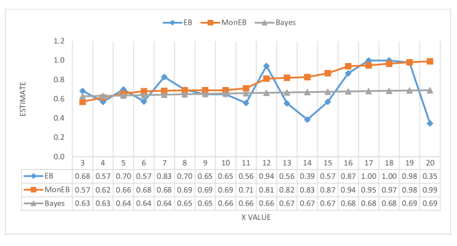
Figure 1: EB, Monotone EB, and Bayesian estimates based on one simulation for $n=500$, $r=3$, and prior $U(0.5,0.8)$.

Now adopt the EB framework. Consider $n=100$ independent copies

$$(X_{1},\Theta_{1}),(X_{2},\Theta_{2}),\ldots,(X_{100},\Theta_{100})$$ (6)

of the random pair $(X,\Theta)$, where $\Theta$ is an uniform $(0.5,0,8)$ variable and, given $\Theta$, $X$ has the BT distribution (1). Assume that $X_{i}$ for $1\leq i\leq 100$ are observable, but $\Theta_{i}$ for $1\leq i\leq 100$ are not observable. For our simulation study, we draw 10 sets like (6). For the $k^{th},1\leq k\leq 10$, set, the EB estimate $\theta^{(k)}_{100}(x)$ is calculated. The value of $S(\theta_{100})$ is estimated by the average (for the 10 samples) $\hat{S}(\theta_{100}):={\displaystyle\frac{1}{10}\sum_{k=1}^{10}S(\theta^{(k)}_{100})}$ and the standard error is calculated. Next, the EB estimator is monotonized and the estimate $\theta^{\ast(k)}_{100}(x)$ is computed. Similarly to $S(\theta_{100})$, we estimate $S(\theta_{100}^{\ast})$ by the average $\hat{S}(\theta_{100}^{\ast})$. The entire procedure is repeated with $n=500$ in (6). The numerical results are given in Table 1. The improvement of $\theta_{n}^{\ast}$ over $\theta_{n}$ is quite substantial. It is surprising that even in the case $n=500$, $\theta_{n}$ lacks monotonicity completely. To give more insight, the complete results for one set (6) of size $n=500$ are presented in Figure 1.

Acknowledgements The first author was partially supported by the NFSR at the MES of Bulgaria, Grant No DFNI-I02/17 while being on leave from the Institute of Mathematics and Informatics at the Bulgarian Academy of Sciences.

References

- [1] Aldous D.J. (1999). Deterministic and stochastic models for coalescence (aggregation and coagulation): a review of the mean-field theory for probabilists. Bernoulli. vol. 5, pp. 3-48.
- [2] Consul P.C., Famoye, F. (2006). Lagrangian Probability Distributions. Birkhauser, Boston.
- [3] Dion J.-P. (1972). Estimation des probabilit6s initiales et de la moyenne d’un processus de Galton-Watson. Ph.D. Thesis, University of Montreal, Montreal.
- [4] Farrington C.P., Kanaan C.P., Gay N.J. (2003). Branching process models for surveillance of infectious diseases controlled by mass vaccination. Biostatistics. vol. 4, pp. 279-295.
- [5] Guttorp P. (1991). Statistical Inference for Branching Processes. Wiley, New York.
- [6] Heyde C.C. (1979). On assessing the potential severity of an outbreak of a rare infectious disease: a Bayesian approach. Austral. J. Statist.. vol. 21, pp. 282-292.
- [7] Jagers P. (1975). Branching Processes with Biological Application. Wiley, London.
- [8] Koorey G. (2007). Passing opportunities at slow-vehicle bays. J. Transportation Engineering. 133, pp. 129-137.
- [9] Liang T. (2009). Empirical Bayes estimation for Borel-Tanner distributions. Stat. and Probab. Lett.. 79, pp. 2212-2219.
- [10] Moll V.H. (2015). Special Integrals of Gradshteyn and Ryzhik the Proofs, Vol. 1. Taylor and Francis, New York.
- [11] Nirei M., Stamatiou T., Sushko V. (2012). Stochastic Herding in Financial Markets Evidence from Institutional Investor Equity Portfolios. BIS Working Papers, No 371.
- [12] Ren H, Xiong J., Watts D., Zhao Y. (2013). Branching Process based Cascading Failure Probability Analysis for a Regional Power Grid in China with Utility Outage Data. Energy and Power Engineering. vol. 5, pp. 914-921.
- [13] Sellke S., Shroff N., Bagchi S.B. (2005). Modeling and automated containment of worms. CERIAS Tech. Report 2005-88. Center for Education and Research in Information Assurance and Security, Purdue University, West Lafayette, IN.
- [14] Van Houwelingen J.C. (1977). Monotonizing empirical Bayes estimators for a class of discrete distributions with monotone likelihood ratio. Statistica Neerlandica. vol. 31, pp. 95-104.