Capacity bounds for distributed storage

Abstract

One of the primary objectives of a distributed storage system is to reliably store large amounts of source data for long durations using a large number $N$ of unreliable storage nodes, each with ${\rm clen}$ bits of storage capacity. Storage nodes fail randomly over time and are replaced with nodes of equal capacity initialized to zeroes, and thus bits are erased at some rate ${\cal E}$. To maintain recoverability of the source data, a repairer continually reads data over a network from nodes at a rate ${\cal R}$, and generates and writes data to nodes based on the read data.

The distributed storage source data capacity is the maximum amount of source data that can be reliably stored for long periods of time. We prove the distributed storage source data capacity asymptotically approaches

$$\left(1-\frac{{\cal E}}{2\cdot{\cal R}}\right)\cdot N\cdot{\rm clen}$$ (1)

as $N$ and ${\cal R}$ grow.

Equation (1) expresses a fundamental trade-off between network traffic and storage overhead to reliably store source data.

I Overview of practical systems

A distributed storage system generically consists of interconnected storage nodes, where each node can store a large quantity of data. A primary goal of a distributed storage system is to reliably store as much source data as possible for a long time.

Commonly, distributed storage systems are built using relatively inexpensive and generally not completely reliable hardware. For example, nodes can go offline for periods of time (transient failure), in which case the data they store is temporarily unavailable, or permanently fail, in which case the data they store is permanently erased. Permanent failures are not uncommon, and transient failures are frequent.

Although it is often hard to accurately model failures, an independent failure model can provide insight into the strengths and weaknesses of a practical system, and can provide a first order approximation to how a practical system operates. In fact, one of the primary reasons practical storage systems are built using distributed infrastructure is so that failures of the infrastructure are as independent as possible.

Distributed storage systems generally allocate a fraction of their capacity to storage overhead, which is used to help maintain recoverability of source data as failures occur. Redundant data, which can be used to help recover lost source data, is generated from source data and stored in addition to source data. A repairer reads stored data to regenerate and restore lost data as failures occur.

For practical systems, source data is generally maintained at the granularity of objects, and erasure codes are used to generate redundant data for each object. For a $(n,k,r)$ erasure code, each object is segmented into $k$ source fragments, an encoder generates $r=n-k$ repair fragments from the $k$ source fragments, and each of these $n=k+r$ fragments is stored at a different node. An erasure code is MDS (maximum distance separable) if the object can be recovered from any $k$ of the $n$ fragments.

Replication is an example of a trivial MDS erasure code, i.e., each fragment is a copy of the original object. For example, triplication can be thought of as using the simple $(3,1,2)$ erasure code, wherein the object can be recovered from any one of the three copies. Many distributed storage systems use replication.

Reed-Solomon codes [2], [3], [5] are MDS codes that are used in a variety of applications and are a popular choice for storage systems. For example, [22] and [19] use a $(9,6,3)$ Reed-Solomon code, and [24] uses a $(14,10,4)$ Reed-Solomon code. These are examples of small code systems, i.e., systems that use small values of $n$, $k$ and $r$.

Since a small number $r+1$ of failures can cause source data loss for small code systems, reactive repair is used, i.e., the repairer operates as quickly as practical to regenerate fragments lost from a node that permanently fails before another node fails, and typically reads $k$ fragments to regenerate each lost fragment. Thus, the peak read rate is higher than the average read rate, and the average read rate is $k$ times the failure erasure rate.

As highlighted in [24], the read rate needed to maintain source data recoverability for small code systems can be substantial. Modifications of standard erasure codes have been designed for storage systems to reduce this rate, e.g., local reconstruction codes [20], [24], and regenerating codes [14], [17]. Some versions of local reconstruction codes have been used in deployments, e.g., by Microsoft Azure.

There are additional issues that make the design of small code systems complicated. For example, placement groups, each mapping $n$ fragments to $n$ of the $N$ nodes, are used to determine where fragments for objects are stored. An equal amount of object data should be assigned to each placement group, and an equal number of placement groups should map a fragment to each node. For small code systems, Ceph [29] recommends $\frac{100\cdot N}{n}$ placement groups, i.e., 100 placement groups map a fragment to each node. A placement group should avoid mapping fragments to nodes with correlated failures, e.g., to the same rack. Pairs of placement groups should avoid mapping fragments to the same pair of nodes. Placement groups are continually remapped as nodes fail and are added. These and other issues make the design of small code systems challenging.

The paper [30] introduces liquid systems, which use erasure codes with large values of $n$, $k$ and $r$. For example, $n=N$ and a fragment is assigned to each node for each object, i.e., only one placement group is used for all objects. The RaptorQ code [4], [6] is an example of an erasure code that is suitable for a liquid system, since objects with large numbers of fragments can be encoded and decoded efficiently in linear time.

Typically $r$ is large for a liquid system, thus source data is unrecoverable only when a large number of nodes fail. A liquid repairer is lazy, i.e., repair operates to slowly regenerate fragments erased from nodes that have permanently failed. The repairer reads $k$ fragments for each object to regenerate around $r$ fragments erased over time due to failures, and the peak read rate is close to the average read rate. The peak read rate for the liquid repairer described in Section VI, is within a factor of two of the lower bounds on the read rate, and the peak read rate for the advanced liquid repairer described in Section VII asymptotically approaches the lower bounds.

There are a number of possible strategies beyond those outlined above that could be used to implement a distributed storage system. One of our primary contributions is to provide fundamental lower bounds on the read rate needed to maintain source data recoverability for any distributed storage system, current or future, for a given storage overhead and failure rate.

II Distributed storage model

We introduce a model of distributed storage which is inspired by properties inherent and common to systems described in Section I. This model captures some of the essential features of any distributed storage system. All lower bounds are proved with respect to this model.

II-A Architecture

Figure 1 shows an architectural overview of the distributed storage model. A storer generates data from source data $x\in\{0,1\}^{\rm xlen}$ received from a source, and stores the generated data at nodes. In our model we assume the source data is randomly and uniformly chosen, and let random variable $X\in_{\cal U}\{0,1\}^{\rm xlen}$, where $\in_{\cal U}$ indicates randomly and uniformly chosen. Thus, $\lvert\lvert{X}\rvert\rvert=\mathbf{H}\left({X}\right)={\rm xlen}$, where $\lvert\lvert{X}\rvert\rvert$ is the length of $X$ and $\mathbf{H}\left({X}\right)$ is the entropy of $X$.

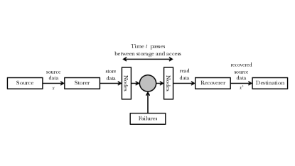
Figure 1: Distributed storage architecture

Figure 2 shows the nodes of the distributed storage system, together with the network that connects each node to a repairer. Each of $N$ nodes $C_{0},\ldots,C_{N-1}$ can store ${\rm clen}$ bits, and the capacity is $N\cdot{\rm clen}$. The storage overhead $\beta$ is the fraction of capacity available beyond ${\rm xlen}$, i.e.,

$$\beta=1-\frac{{\rm xlen}}{N\cdot{\rm clen}},$$ (2)

thus ${\rm xlen}=(1-\beta)\cdot N\cdot{\rm clen}$.

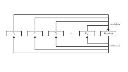
Figure 2: Storage nodes and repairer model.

As nodes fail and are replaced, a repairer continually reads data from the nodes, computes a function of the read data, and writes the computed data back to the nodes. The repairer tries to ensure that the source data can be recovered at any time from the data stored at the nodes.

As shown in Figure 1, after some amount of time $t$ passes, a recoverer reads data from the nodes to generate $x^{\prime}$, which is provided to a destination, where $x$ is reliably recovered if $x^{\prime}=x$. The goal is to maximize the amount of time $t$ the recoverer can reliably recover $x$.

II-B Failures

A failure sequence determines when and what nodes fail as time passes. A failure sequence is a combination of two sequences, a timing sequence

$$t_{0}\leq t_{1}\leq\cdots\leq t_{i}\cdots,$$

where for index $i$, $t_{i}$ is the time at which a node fails, and an identifier sequence

$$y_{0},y_{1},\ldots,y_{i},\ldots,$$

where $y_{i}$ is the identifier of the node that fails at time $t_{i}$.

All ${\rm clen}$ bits stored at node $y_{i}$ are immediately erased at time $t_{i}$ when the node fails, i.e., all ${\rm clen}$ bits of node $y_{i}$ are initialized to zero at time $t_{i}$ when the node fails. This can be viewed as immediately replacing a failed node with a replacement node with storage initialized to zeroes. Thus, at each time there are $N$ nodes.

A primary objective of practical distributed storage architectures is to distribute the components of the system so that failures are as independent as possible. Poisson failure distributions are an idealization of this primary objective, and are often used to model and evaluate distributed storage systems in practice. For a Poisson failure distribution with rate $\lambda$, the time between when a node is initialized and when it fails is an exponential random variable with rate $\lambda$, i.e., $\frac{1}{\lambda}$ is the average lifetime of a node between when it is initialized and when it fails. Our main lower bounds in Section V are with respect to Poisson failure distributions.

II-C Network

The model assumes there is a network interface between each node and the system over which all data from and to the node travels. One of the primary lower bound metrics is the amount of data that travels over interfaces from nodes to the system, which is counted as data read by the system. For the lower bounds, this is the only network traffic that is counted. All other data traffic within the system, i.e. data traffic across the system, data traffic over an interface from the system to nodes, or any other data traffic that does not travel over an interface from a node to the system, is not counted for the lower bounds. It is assumed that the network is completely reliable, and that all data that travels over an interface from a node to the system is instantly available everywhere within the system.

II-D Storer

A storer takes the source data $x$ and generates and stores data at the nodes in a preprocessing step when the system is first initialized and before there are any failures. We assume that the recoverer can reliably recover $x$ from the data stored at the nodes immediately after the preprocessing step finishes.

For simplicity, we view the storer preprocessing step as part of the repairer, and any data read during the storer preprocessing step is not counted in the lower bounds.

For the lower bounds, there are no assumptions about how the storer generates the stored data from the source data, i.e. no assumptions about any type of coding used, no assumptions about partitioning the source data into objects, etc. As an example, the source data can be encrypted, compressed, encoded using an error-correcting code or erasure code, replicated, or processed in any other way known or unknown to generate the stored data, and still the lower bounds hold. Analogous remarks hold for the repairers described next.

II-E Repairer

A repairer ensures that the source data is recoverable when data generated from the source data is stored at the unreliable nodes. A repairer for a system operates as follows. The identifier $y_{i}$ is provided to a repairer at time $t_{i}$, which alerts the repairer that all ${\rm clen}$ bits stored on node $y_{i}$ are lost at that time. As nodes fail and are replaced, the repairer reads data over interfaces from nodes, performs computations on the read data, and writes computed data over interfaces to nodes. A primary metric is the number of bits the repairer reads over interfaces from storage nodes.

Let ${\rm Lseq}(t)=({\rm tseq},{\rm yseq})$ be the failure sequence up till time $t$, where ${\rm tseq}=\{t_{0},\ldots,t_{\ell}\},$ ${\rm yseq}=\{y_{0},\ldots,y_{\ell}\},$ and $\ell=\operatorname*{arg\,max}_{i}\{t_{i}\leq t\}$. The repairer ${\mathbf{R}}$ has access to ${\rm Lseq}(t)$ at time $t$ at no cost.

Let $V(t)$ be the bits stored in the global memory of ${\mathbf{R}}$, where ${\rm vlen}=\lvert\lvert{V(t)}\rvert\rvert$,

$$C_{0}(t),\ldots,C_{N-1}(t)$$

be the bits stored at nodes $0,\ldots,N-1$, respectively, where ${\rm clen}=\lvert\lvert{C_{j}(t)}\rvert\rvert$ is the capacity of each node $j$, and

$$S(t)=\{V(t),\{C_{0}(t),\ldots,C_{N-1}(t)\}\}$$

is the global state of the system at time $t$, where ${\rm slen}=\lvert\lvert{S(t)}\rvert\rvert$. Thus,

$${\rm slen}={\rm vlen}+N\cdot{\rm clen}$$

is the size of the global system state at any time $t$.

The actions of ${\mathbf{R}}$ at time $t$ are determined by $(t,V(t),{\rm Lseq}(t))$. If a node $j$ fails at time $t$ then ${\mathbf{R}}$ is notified at time $t$ that node $j$ failed and ${\rm Lseq}(t)$ is updated. If ${\mathbf{R}}$ reads data over the interface from node $j$ at time $t$ (when to read from node $j$ is determined by $(t,V(t),{\rm Lseq}(t))$) then the amount and location of the data read from $C_{j}(t)$ is determined by $(t,V(t),{\rm Lseq}(t))$. The data read over the interface from node $j$ in response to a request initiated at time $t$ is assumed to be instantaneously available, i.e. all of the requested data is available at time $t$ over the interface from node $j$.

$V(t)$ can be used by the repairer to store the programs the repairer executes, store information from the past, temporarily store data read from nodes, perform computations on read data, temporarily store computed data before it is written to nodes, and generally to store any information the repairer needs immediate access to that is not stored at the nodes. The distinction between $V(t)$ and the nodes is that $V(t)$ is persistent memory (not subject to any type of failure in the model) and available globally to ${\mathbf{R}}$ (there is no read or write cost for accessing $V(t)$). ${\mathbf{R}}$ can also store such information at the nodes, but this information is subject to loss due to possible failures.

Repairers are allowed to use an unbounded amount of computation, since computation time is not a metric of interest in the lower bounds. The granularity of how much data is read or written in one step is unconstrained, e.g. one bit or Terrabytes of data can be read over an interface from a node during a read step, and the lower bounds still hold. The granularity of the timing of read and write steps is also unconstrained, e.g. there may be a read step each nanosecond, or every twenty minutes.

Local-computation repairers, inspired by [14] and [17], are more powerful than repairers. The motivation for the local-computation repairer model is that a node often has CPUs, memory and storage, and often the impact of traffic between storage and memory at a node is much less than the impact of traffic over the interface from the node to the system. Thus, an arbitrary amount of data may be accessed locally from storage into local memory at a node, local CPUs may compute and store in the local memory a much smaller amount of data from the data accessed into local memory, and it is the much smaller amount of data computed by the CPUs that is sent over the interface from the node to the system. The model does not count the data accessed from storage into local memory, it only counts the data in the local memory that is read by the system over the interface from the node.

Formally, for a local-computation repairer, when data is to be read over the interface from node $j$ initiated at time $t$ (when to read from node $j$ is determined by $(t,V(t),{\rm Lseq}(t))$), a copy of the entire global memory of the local-computation repairer is assumed to be instantaneously available in the local memory at node $j$ at no cost. As the local computation at node $j$ progresses, the copy may evolve to be different than the global memory of the local-computation repairer at time $t$, but the only information the local-computation repairer potentially receives about any changes to the copy in the local memory is from the locally computed data read by the local-computation repairer over the interface from node $j$. The locally computed data is generated based on $(t,V(t),{\rm Lseq}(t),C_{j}(t))$, and then the locally computed data is read by the local-computation repairer over the interface from node $j$. The local computational power at node $j$ and the throughput of the interface at node $j$ are assumed to be unlimited, and thus the locally computed data requested at time $t$ by the local-computation repairer is available instantly at time $t$ over the interface from node $j$.

Thus the data read over the interface from node $j$ when the request for the data is initiated at time $t$ is determined by $(t,V(t),{\rm Lseq}(t),C_{j}(t))$. In this model only the locally computed data is counted as data read over the interface from node $j$; the data accessed from storage at node $j$ to produce the locally computed data (which could be all of $C_{j}(t)$) is not counted.

For example, in the extreme a local-computation repairer could locally access all data stored at a node to produce $1$ KB of locally computed data, and then only the $1$ KB of locally computed data is read over the interface from the node. In this example, only $1$ KB of data is counted towards data read by the local-computation repairer. Thus there is a significant cost to this generalization that is not counted in the amount of data read from nodes by the repairer. These issues are discussed in more detail in Section VIII.

A repairer is a special case of a local-computation repairer: a repairer is simply a local-computation repairer where the data accessed from storage at the node is directly sent over the interface from the node to the repairer.

A repairer may employ a randomized algorithm, which could be modeled by augmenting the repairer with random and independently chosen bits. However, since the repairer is deterministic for a fixed setting of the random bits and the lower bounds hold for any deterministic repairer, the same lower bounds hold for any randomized repairer. Thus, we describe lower bounds only for deterministic repairers, noting that all the lower bound results immediately carry over to randomized repairers.

II-F Recoverer

For any repairer ${\mathbf{R}}$ there is a recoverer ${\mathbf{A}}$ such that if the source data is $x$ and the state at time $t$ is $S(t)$ when the repairer is ${\mathbf{R}}$ then ${\mathbf{A}}(S(t))$ should be equal to $x$.

Source data $x$ is recoverable at time $t$ with respect to repairer ${\mathbf{R}}$ and recoverer ${\mathbf{A}}$ if ${\mathbf{A}}(S(t))=x$. Source data $x$ is unrecoverable at time $t$ with respect to repairer ${\mathbf{R}}$ and recoverer ${\mathbf{A}}$ if ${\mathbf{A}}(S(t))\not=x$.

II-G Applying the lower bounds to real systems

The description of the model makes some very unrealistic assumptions about how real systems operate in practice. However, it is these assumptions that ensure that the lower bounds apply to all real systems. Consider a real system where nodes fail randomly as in the model, but also portions of the network intermittently fail, network bandwidth availability is limited and varying between different parts of the system, memory is not completely reliable, multiple distributed semi-autonomous processes are interacting with different sets of nodes, responses are not immediate to data requests over node interfaces, processes are not immediately notified when nodes fail, notification of node failure is not global, nodes are not immediately replaced, computational resources are limited, etc. We describe an omniscient agent acting with respect to the model in the role of the repairer, where the agent emulates the processes and behaviors of the real system. This shows the lower bounds also apply to the real system.

In the model, nodes that fail are immediately replaced and the agent is immediately notified. In the real system, a failed node may not be replaced immediately. Thus, to emulate the real system, the agent disallows any response to a request to read or write data to a failed node from a process until the time when the node would have been replaced in the real system.

In the real system, notifications of node failures may not be instantaneous, and only some processes may be notified. Thus, the agent only notifies the appropriate processes of node failures when they would have been notified in the real system.

In the model, the agent receives an immediate and complete response to a request for data over an interface to a node. In the real system, interfaces can have a limited amount of bandwidth, and there can be delays in delivering responses to requests for data by processes over a node interface due to computational limits or other constraints. Thus, the agent delivers data to requesting processes with the delays and at the speed of the real system.

In the real system, only a small portion of the global memory state may be available in the local memory of a node when local-computation repair is used. Thus, the agent may only need a small portion of the global memory at the node to emulate a local-computation repairer of the real system.

In the model, the agent acting as a repairer has one global memory. In the real system, repair may be implemented by a distributed set of processes ${\mathbf{R}}_{1},\ldots,{\mathbf{R}}_{i}$ executing concurrent reads and writes over node interfaces, each with their own private memory $V_{1}(t),\ldots,V_{i}(t)$ at time $t$. The agent ${\mathbf{R}}$ can emulate ${\mathbf{R}}_{1},\ldots,{\mathbf{R}}_{i}$ as follows. The global memory of ${\mathbf{R}}$ is

$$V(t)=\{V_{1}(t),\ldots,V_{i}(t)\}.$$

If processes ${\mathbf{R}}_{i}$ and ${\mathbf{R}}_{j}$ send bits between their local memories at time $t$ then these same bits are copied between $V_{i}(t)$ and $V_{j}(t)$ by ${\mathbf{R}}$ at time $t$. The movement of data between the local memories of the processes that the agent is emulating is at no cost. Thus, the lower bound on the amount of data read over interfaces from nodes by ${\mathbf{R}}$ in the model is a lower bound on the amount of data read over interfaces from nodes by ${\mathbf{R}}_{1},\ldots,{\mathbf{R}}_{i}$.

In the model, the agent has a single interface with each node. In the real system, a node can have multiple interfaces. These multiple interfaces are considered as one logical interface by the agent when counting the amount of data traveling over interfaces from nodes to the agent, and the agent delivers data traveling over the multiple interfaces to the appropriate requesting processes of the emulated real system.

The count of data traffic for the lower bounds is conservative, i.e. the amount of data that travels over interfaces from nodes to the agent is a lower bound on the amount of data traveling over the network in the real system.

Thus, a real system, whether it is perfectly architected and has non-failing infinite network bandwidth, zero computational delays, instant node failure notification, or whether it is more realistic as described above, can be emulated by the agent in the model as described above. Since the lower bounds apply to the agent with respect to the model, the lower bounds also apply to any real system.

II-H Practical parameters example

A practical system can have $N=10^{5}$ nodes, ${\rm clen}=10^{16}$ bits of capacity at each node, thus $N\cdot{\rm clen}=10^{21}$. The amount of storage needed by the repairer to store its programs and state generously is at most something like ${\rm vlen}=10^{13}$ bits. Generally, ${\rm clen}>>{\rm vlen}>>N$. We assume ${\rm clen}\geq N$ and ${\rm vlen}<<N\cdot{\rm clen}$ in our bounds with respect to growing $N$.

Practical values of $\beta$ range from $2/3$ (triplication) to $1/20$ and smaller. In the example, ${\rm xlen}=(1-\beta)\cdot N\cdot{\rm clen}\approx 10^{21}$. In practice nodes fail each few years, e.g., $1/\lambda=$ 3 years.

III Emulating repairers in phases

We prove lower bounds based on considering the actions of a repairer ${\mathbf{R}}$, or local-computation repairer ${\mathbf{R}}$, running in phases on a failure sequence. Each phase considers a portion of a failure sequence with $M$ failures, where each of the $M$ failures within a phase are distinct, as described in more detail below.

For any $M\leq N$, we write

$$\langle{y_{0},\ldots,y_{M-1}}\rangle$$

when all identifiers are distinct, i.e., $y_{i}\not=y_{i^{\prime}}$ for $0\leq i\not=i^{\prime}\leq M-1$. We write

$$\langle{y_{0},\ldots,y_{j-1},Y_{j},\ldots,Y_{M-1}}\rangle$$

when $\langle{y_{0},\ldots,y_{j-1}}\rangle$ are distinct identifiers, random variable $Y_{j}$ is defined as

$$Y_{j}\in_{\cal U}\{0,\ldots,N-1\}-\{y_{0},\ldots,y_{j-1}\},$$

and for $i=j+1,\ldots,M-1$, random variable $Y_{i}$ is defined as

$$Y_{i}\in_{\cal U}\{0,\ldots,N-1\}-\{y_{0},\ldots,y_{j-1},Y_{j},\ldots Y_{i-1}\},$$

where $\in_{\cal U}$ indicates randomly and uniformly chosen. Thus, $\langle{y_{0},\ldots,y_{j-1},Y_{j},\ldots,Y_{M-1}}\rangle$ is a distribution on distinct identifiers.

A phase consists of executing ${\mathbf{R}}$ on a portion of a failure sequence $({\rm tseq},{\rm yseq})$, where

$${\rm tseq}=\{t_{0},t_{1},\ldots,t_{M-1}\}$$

is the portion of the timing sequence and

$${\rm yseq}=\langle{y_{0},y_{1},\ldots,y_{M-1}}\rangle$$

is the portion of the identifier sequence that is revealed to ${\mathbf{R}}$ as the phase progresses.

Before a phase begins, the storer generated and stored data at the nodes based on source data $x$, and the repairer ${\mathbf{R}}$ has been executed with respect to a failure sequence up till time $t^{\scaleto{-}{4pt}}_{0}$, where $t^{\scaleto{-}{4pt}}_{0}$ is just before the time of the first failure of the phase at time $t_{0}$. We assume that the recoverer ${\mathbf{A}}$ can recover source data $x$ from the state $S(t^{\scaleto{-}{4pt}}_{0})$.

Conceptually, there are two executions of ${\mathbf{R}}$ on $({\rm tseq},{\rm yseq})$ in a phase. The first execution runs ${\mathbf{R}}$ normally from $t^{\scaleto{-}{4pt}}_{0}$ to $t^{\scaleto{+}{4pt}}_{M-1}$ starting system state $S(t^{\scaleto{-}{4pt}}_{0})$ and ending in $S(t^{\scaleto{+}{4pt}}_{M-1})$, where $t^{\scaleto{-}{4pt}}_{0}$ is just before $t_{0}$, and $t^{\scaleto{+}{4pt}}_{M-1}$ is just after $t_{M-1}$. Thus, the failures at times $t_{0}$ and $t_{M-1}$ are within the phase, but ${\mathbf{R}}$ does not read any bits before $t_{0}$ or after $t_{M-1}$ in the phase.

The following compressed state is defined by the first execution of ${\mathbf{R}}$. For $i=1,\ldots,M-1$, let $R_{y_{i}}$ be the concatenation of the bits read by repairer ${\mathbf{R}}$ over the interface from node $y_{i}$ between $t_{0}$ and $t_{i}$. More generally, if ${\mathbf{R}}$ is a local-computation repairer, then $R_{y_{i}}$ is the concatenation of the locally-computed bits read by ${\mathbf{R}}$ over the interface from node $y_{i}$ between $t_{0}$ and $t_{i}$. Let

$$D=\{V(t^{\scaleto{-}{4pt}}_{0}),\{C_{j}(t^{\scaleto{-}{4pt}}_{0}):j\not\in{\rm yseq}\},\{R_{j}:j\in{\rm yseq}\}\}$$

be the compressed state with respect to $(x,({\rm tseq},{\rm yseq}))$. The first execution of ${\mathbf{R}}$ shows that $D$ can be generated based on repairer ${\mathbf{R}}$, $S(t^{\scaleto{-}{4pt}}_{0})$ and $({\rm tseq},{\rm yseq})$.

The second execution uses the compressed state $D$ in place of $S(t^{\scaleto{-}{4pt}}_{0})$ to emulate ${\mathbf{R}}$ on $({\rm tseq},{\rm yseq})$ and arrive in the same final state $S(t^{\scaleto{+}{4pt}}_{M-1})$ as the first execution. The initial memory state of ${\mathbf{R}}$ is set to $V(t^{\scaleto{-}{4pt}}_{0})$ and the state of node $j$ is initialized to $C_{j}(t^{\scaleto{-}{4pt}}_{0})$ for all $j\notin{\rm yseq}$. Function $f:\{0,\ldots,N-1\}\rightarrow\{0,1\}$ is initialized as follows: $f(j)=1$ if $j\in{\rm yseq}$ and $f(j)=0$ if $j\not\in{\rm yseq}$. ${\mathbf{R}}$ is emulated from $t^{\scaleto{-}{4pt}}_{0}$ to $t^{\scaleto{+}{4pt}}_{M-1}$ the same as in the first execution with the following differences. When ${\mathbf{R}}$ is to read bits over the interface from node $j$ at time $t$: if $f(j)==0$ then the requested bits are read from $S_{j}(t)$; if $f(j)==1$ then the requested bits are provided to ${\mathbf{R}}$ from the next portion of $R_{j}$ not yet provided to ${\mathbf{R}}$. When ${\mathbf{R}}$ is to write bits to a node $j$ at time $t$: if $f(j)==0$ then the bits are written to $S_{j}(t)$; if $f(j)==1$ then the write is skipped. At time $t$ when $j\in{\rm yseq}$ first fails within the phase, $f(j)$ is reset to $0$ and $S_{j}(t)$ is initialized to all zero bits.

If ${\mathbf{R}}$ is a local-computation repairer instead of a repairer then when ${\mathbf{R}}$ is to produce and read locally-computed bits over the interface from node $j$ at time $t$ and $f(j)==0$ the requested bits are locally-computed by ${\mathbf{R}}$ based also on $C_{j}(t)$.

It can be verified that the state of the system is $S(t^{\scaleto{+}{4pt}}_{M-1})$ at the end of the emulation, whether ${\mathbf{R}}$ is a repairer or a local-computation repairer. Thus, $(S(t^{\scaleto{+}{4pt}}_{M-1}),({\rm tseq},{\rm yseq}))$ can be generated from $(D,({\rm tseq},{\rm yseq}))$ based on ${\mathbf{R}}$.

A key intuition is that if repairer ${\mathbf{R}}$ doesn’t read enough data over interfaces from nodes that fail before they fail during a phase then $\lvert\lvert{D}\rvert\rvert<{\rm xlen}$ and thus $x$ cannot be reliably recovered from $D$. On the other hand, $x$ is recoverable at time $t^{\scaleto{+}{4pt}}_{M-1}$ by ${\mathbf{A}}$ only if $x$ can be recovered from $D$ since $D$ can generate $S(t^{\scaleto{+}{4pt}}_{M-1})$ and ${\mathbf{A}}(S(t^{\scaleto{+}{4pt}}_{M-1}))$ is supposed to equal $x$. Thus, if repairer ${\mathbf{R}}$ doesn’t read enough data over interfaces from nodes that fail before they fail during a phase then $x$ is unrecoverable at time $t^{\scaleto{+}{4pt}}_{M-1}$ by ${\mathbf{A}}$. We formalize this intuition below.

We let

$$x\rightarrow_{({\rm tseq},{\rm yseq})}D\rightarrow_{({\rm tseq},{\rm yseq})}x^{\prime}$$

indicate that source data $x$ is mapped before the start of the phase to a value of $S(t^{\scaleto{-}{4pt}}_{0})$ by ${\mathbf{R}}$, which in turn is mapped by $({\rm tseq},{\rm yseq})$ to a value $D$ by the first execution of the emulation of ${\mathbf{R}}$, which is mapped to a value of $S(t^{\scaleto{+}{4pt}}_{M-1})$ by $({\rm tseq},{\rm yseq})$ by the second execution of the emulation of ${\mathbf{R}}$, which in turn is mapped by ${\mathbf{A}}$ to a value $x^{\prime}\in\{0,1\}^{\rm xlen}$.

Compression Lemma III.1

For any repairer or local-computation repairer ${\mathbf{R}}$ and recoverer ${\mathbf{A}}$, for any $({\rm tseq},{\rm yseq})$, for any

$${\cal X}\subseteq{\cal X}_{({\rm tseq},{\rm yseq})}=\left\{x:x\rightarrow_{({\rm tseq},{\rm yseq})}D\in\{0,1\}^{{\rm xlen}-\ell}\right\},$$

$$\mathbf{Pr}_{X,({\rm tseq},{\rm yseq})}\left[{(X\in{\cal X})\wedge(X\mbox{ \rm recoverable at }t^{\scaleto{+}{4pt}}_{M-1})}\right]$$

$$\leq 2^{-\ell}.$$

Proof:

For any $({\rm tseq},{\rm yseq})$, for any ${\cal X}\subseteq{\cal X}_{({\rm tseq},{\rm yseq})}$, for any $x\in{\cal X}$,

$$x\rightarrow_{({\rm tseq},{\rm yseq})}D\rightarrow_{({\rm tseq},{\rm yseq})}x^{\prime}$$

for some $D\in\{0,1\}^{{\rm xlen}-\ell}$ and some $x^{\prime}\in\{0,1\}^{\rm xlen}$. Since $D\in\{0,1\}^{{\rm xlen}-\ell}$, the number of possible $x^{\prime}$ values is at most $2^{{\rm xlen}-\ell}$, thus $x=x^{\prime}$ for at most $2^{{\rm xlen}-\ell}$ of the $x\in{\cal X}$. ∎∎

Let

$${\rm ulen}=\sum_{j\in{\rm yseq}}\lvert\lvert{R_{j}}\rvert\rvert$$ (3)

with respect to $(x,({\rm tseq},{\rm yseq}))$ be the total length of data read by ${\mathbf{R}}$ from nodes that fail before their failure in the phase. Then,

$$\lvert\lvert{D}\rvert\rvert={\rm vlen}+(N-M)\cdot{\rm clen}+{\rm ulen}$$ (4)

with respect to $(x,({\rm tseq},{\rm yseq}))$. Let

$${\rm olen}=N\cdot{\rm clen}-{\rm xlen}+{\rm vlen}+1,$$ (5)

and let

$$F=\left\lceil\frac{{\rm olen}}{s}\right\rceil$$ (6)

be the minimal number of nodes so that $F\cdot{\rm clen}\geq{\rm olen}$. Let

$${\beta^{\prime}}=\frac{F}{N}$$ (7)

Note that

$$\beta\leq{\beta^{\prime}}\leq\beta+\frac{{\rm vlen}+1}{N\cdot{\rm clen}}+\frac{1}{N}.$$

Generally, ${\beta^{\prime}}\approx\beta$, e.g., for the practical system described in Subsection II-H, ${\beta^{\prime}}\leq\beta+10^{-7}+10^{-4}$.

Hereafter we set $M=2\cdot F<N$, which implies ${\beta^{\prime}}<1/2$. This restriction is mild since ${\beta^{\prime}}\rightarrow 0$ is more interesting in practice than ${\beta^{\prime}}\approx 1$.

Compression Corollary III.2

For any repairer or local-computation repairer ${\mathbf{R}}$ and recoverer ${\mathbf{A}}$, for any $({\rm tseq},{\rm yseq})$, for any

$${\cal X}\subseteq{\cal X}_{({\rm tseq},{\rm yseq})}=\left\{x:{\rm ulen}\leq(F-1)\cdot{\rm clen}\right\}$$

where ${\rm ulen}$ is defined with respect to $(x,({\rm tseq},{\rm yseq}))$,

$$\mathbf{Pr}_{X,({\rm tseq},{\rm yseq})}\left[{(X\in{\cal X})\wedge(X\mbox{ \rm recoverable at }t^{\scaleto{+}{4pt}}_{M-1})}\right]$$ (8)

$$\leq 2^{-{\rm clen}}.$$

Proof:

Follows from Compression Lemma III.1 with $M=2\cdot F\leq N$, $\ell={\rm clen}$, and using Equations (4), (5), (6). ∎∎

Note that $2^{-{\rm clen}}$ is essentially zero in any practical setting. For example, $2^{-{\rm clen}}\leq 10^{-3\cdot 10^{15}}$ for the settings in Section II-H.

Note that Compression Lemma III.1 and Compression Corollary III.2 rely upon the assumption that the source data is uniformly distributed, and this is the root of the dependency of all subsequent technical results on this assumption.

A natural relaxation of this assumption is that the source data has high min-entropy, where the min-entropy is the log base two of one over the probability of $x$, where $x$ is the most likely value for the source data. Thus the min-entropy of the source data is always at most ${\rm xlen}$.

Since the source data for practical systems is composed of many independent source objects, typically the min-entropy of the source data for a practical system is close to ${\rm xlen}$. It can be verified that all of the lower bounds hold if the min-entropy of the source data is universally substituted for ${\rm xlen}$.

IV Core lower bounds

From Compression Corollary III.2, a necessary condition for source data $x$ to be reliably recoverable at the end of the phase is that repairer or local-computation repairer ${\mathbf{R}}$ must read a lot of data from nodes that fail during the phase, and ${\mathbf{R}}$ must read this data before the nodes fail.

On the other hand, ${\mathbf{R}}$ cannot predict which nodes are going to fail during a phase, and only a small fraction of the nodes fail during a phase. Thus, to ensure that enough data has been read from nodes that fail before the end of the phase, a larger amount of data must be read in aggregate from all the nodes.

Core Lemma IV.1, the primary technical contribution of this section, is used to prove Core Theorem IV.2 and all later results.

Fix $x$, ${\rm tseq}=\{t_{0},\ldots,t_{M-1}\}$, and ${\rm yseq}=\langle{y_{0},\ldots,y_{M-1}}\rangle$.

For $i\in\{0,\ldots,M-1\}$, let ${\rm tseq}_{i}=\{t_{0},\ldots,t_{i}\}$ be a prefix of ${\rm tseq}$, and let ${\rm yseq}_{i}=\langle{y_{0},\ldots,y_{i}}\rangle$ be a prefix of ${\rm yseq}$. For $i\in\{0,\ldots,M-1\}$, $j\in\{0,\ldots,N-1\}$, let

$${\rm rlen}_{i,j}$$

with respect to $(x,({\rm tseq}_{i},{\rm yseq}_{i-1}))$ be the amount of data read from node $j$ up till time $t_{i}$. For $i\in\{0,\ldots,M-1\}$, let

$${\rm rlen}_{i}=\sum_{j\in\{0,\ldots,N-1\}}{\rm rlen}_{i,j}$$

with respect to $(x,({\rm tseq}_{i},{\rm yseq}_{i-1}))$. Let

$${\rm ulen}_{i}={\rm rlen}_{i,y_{i}}$$

with respect to $(x,({\rm tseq}_{i},{\rm yseq}_{i}))$ be the total number of bits read from the node $y_{i}$ up till it fails at time $t_{i}$. Then,

$${\rm ulen}=\sum_{i=1}^{M-1}{\rm ulen}_{i}$$

with respect to $(x,({\rm tseq},{\rm yseq}))$, where ${\rm ulen}$ is defined in Equation (3).

Core Lemma IV.1

Fix ${\beta^{\prime}}<1/2$. Fix $\epsilon_{c}>0$ and let

$$\delta_{\scriptscriptstyle\rm c}=2\cdot F\cdot e^{-\frac{\epsilon_{c}^{2}\cdot F}{4}+\epsilon_{c}}.$$ (9)

For $i=1,\dots,2\cdot F-1$, let

$$\Gamma_{i}=(1-\epsilon_{c})\cdot\frac{i\cdot\left(N-\frac{i+1}{2}\right)\cdot{\rm clen}}{2\cdot F-1}.$$ (10)

For any repairer or local-computation repairer,

$$\mathbf{Pr}_{x,({\rm tseq},{\rm Yseq})}\left[{\left(\forall_{i=1}^{2\cdot F-1}{\rm rlen}_{i}<\Gamma_{i}\right)\wedge({\rm ulen}>(F-1)\cdot{\rm clen})}\right]$$

$$\leq\delta_{\scriptscriptstyle\rm c},$$

for any $x$ , ${\rm tseq}$, and ${\rm Yseq}=\langle{y_{0},Y_{1}\ldots,Y_{2\cdot F-1}}\rangle$ for any $y_{0}$.

Proof:

Fix $x$, ${\rm tseq}$ and $y_{0}$. The parameterization with respect to $x$ and ${\rm tseq}$ are implicit in the remainder of the proof. Fix $\eta=(F-1)\cdot{\rm clen}$. We first prove that for any repairer or local-computation repairer ${\mathbf{R}^{\prime}}$ there is a repairer or local-computation repairer ${\mathbf{R}}$ such that

$$\mathbf{Pr}\left[{\left(\forall_{i=1}^{2\cdot F-1}{\rm rlen}^{\prime}_{i}<\Gamma_{i}\right)\wedge({\rm ulen}^{\prime}>\eta)}\right]$$ (11)

$$\leq\mathbf{Pr}\left[{{\rm ulen}>\eta}\right]$$

and

$$\mathbf{Pr}\left[{\forall_{i=1}^{2\cdot F-1}{\rm rlen}_{i}<\Gamma_{i}}\right]=1$$ (12)

with respect to $\langle{y_{0},Y_{1}\ldots,Y_{2\cdot F-1}}\rangle$, and where ${\rm rlen}^{\prime}_{i}$ and ${\rm ulen}^{\prime}$ are defined with respect to ${\mathbf{R}^{\prime}}$ and ${\rm rlen}_{i}$ and ${\rm ulen}$ are defined with respect to ${\mathbf{R}}$.

Let predicate $P$ be defined as follows on input $\langle{y_{0},\ldots,y_{M-1}}\rangle$.

$$P\mbox{ \rm is true }\iff\forall_{i=1}^{2\cdot F-1}{\rm rlen}^{\prime}_{i}<\Gamma_{i}$$

with respect to $\langle{y_{0},\ldots,y_{M-1}}\rangle$.

${\mathbf{R}}$ acts the same way as ${\mathbf{R}^{\prime}}$ with respect to $\langle{y_{0},\ldots,y_{M-1}}\rangle$ for which $P$ is true, thus ${\rm rlen}_{i}={\rm rlen}^{\prime}_{i}$ for $i=1,\ldots,M-1$, and ${\rm ulen}={\rm ulen}^{\prime}$, with respect to $\langle{y_{0},\ldots,y_{M-1}}\rangle$ for which $P$ is true.

Fix $\langle{y_{0},\ldots,y_{M-1}}\rangle$ for which $P$ is false, let

$$\ell=\operatorname*{arg\,min}_{i=1,\ldots,M-1}\{{\rm rlen}^{\prime}_{i}\geq\Gamma_{i}\}$$

with respect to $\langle{y_{0},\ldots,y_{M-1}}\rangle$. ${\mathbf{R}}$ acts the same way up till time $t_{\ell-1}$, but doesn’t read data from nodes after $t_{\ell-1}$, with respect to $\langle{y_{0},\ldots,y_{M-1}}\rangle$. Thus, ${\rm rlen}_{i}={\rm rlen}^{\prime}_{i}$ for $i=1,\ldots,\ell-1$, ${\rm rlen}_{i}={\rm rlen}^{\prime}_{\ell-1}$ for $i=\ell,\ldots,M-1$, with respect to $\langle{y_{0},\ldots,y_{M-1}}\rangle$. From this, $\forall_{i=1}^{2\cdot F-1}{\rm rlen}_{i}<\Gamma_{i}$ with respect to any $\langle{y_{0},\ldots,y_{M-1}}\rangle$ for which $P$ is false. Thus, condition (12) holds for repairer ${\mathbf{R}}$.

It can also be verified that ${\rm ulen}={\rm ulen}^{\prime}$ with respect to all $\langle{y_{0},\ldots,y_{M-1}}\rangle$ for which $P$ is true. From this it follows that

$$\mathbf{Pr}\left[{\left(\forall_{i=1}^{2\cdot F-1}{\rm rlen}^{\prime}_{i}<\Gamma_{i}\right)\wedge({\rm ulen}^{\prime}>\eta)}\right]$$

$$=\mathbf{Pr}\left[{P=\mbox{ \rm true }\wedge{\rm ulen}>\eta}\right]$$

$$\leq\mathbf{Pr}\left[{{\rm ulen}>\eta}\right]$$

with respect to $\langle{y_{0},Y_{1}\ldots,Y_{2\cdot F-1}}\rangle$, thus Inequality (11) holds.

The rest of the proof bounds $\mathbf{Pr}\left[{{\rm ulen}>\eta}\right]$ for repairer or local-computation repairer ${\mathbf{R}}$, which provides the bound on Inequality (11). It can be verified that

$$\mathbf{E}\left[{{\rm ulen}_{i}}\right]=\frac{{\rm rlen}_{i}-\sum_{\ell=1}^{i-1}{\rm ulen}_{\ell}}{N-i}$$ (13)

with respect to $\langle{y_{0},\ldots y_{i-1},Y_{i}}\rangle$. Let

$$\rho=\frac{(1-\epsilon_{c})\cdot{\rm clen}}{2\cdot F-1},$$

$$\tau_{i}=\sum_{\ell=1}^{i}\ell=\frac{i\cdot(i+1)}{2}.$$

If

$$\sum_{\ell=1}^{i-1}{\rm ulen}_{\ell}\geq\tau_{i-1}\cdot\rho$$ (14)

with respect to $\langle{y_{0},\ldots,y_{i-1}}\rangle$ then

$$\mathbf{E}\left[{{\rm ulen}_{i}}\right]\leq i\cdot\rho$$ (15)

with respect to $\langle{y_{0},\ldots,y_{i-1},Y_{i}}\rangle$. This follows from Equation (13), Condition (12), Inequality (14), and because

$$\frac{\Gamma_{i}-\tau_{i-1}\cdot\rho}{N-i}=i\cdot\rho.$$

Define $z_{0}=0$, and for $i=1,\ldots,2\cdot F-1$,

$$Z_{i}=z_{i-1}+{\rm ulen}_{i}-i\cdot\rho=\sum_{\ell=1}^{i}{\rm ulen}_{\ell}-\tau_{i}\cdot\rho$$ (16)

with respect to $\langle{y_{0},\ldots,y_{i-1},Y_{i}}\rangle$, and define $z_{i}$ similarly with respect to $\langle{y_{0},\ldots,y_{i-1},y_{i}}\rangle$. It can be verified that

$$\tau_{2\cdot F-1}\cdot\rho=F\cdot{\rm clen}-\epsilon_{c}\cdot F\cdot{\rm clen}=\eta-(\epsilon_{c}\cdot F-1)\cdot{\rm clen},$$

thus

$$\mathbf{Pr}\left[{Z_{2\cdot F-1}>(\epsilon_{c}\cdot F-1)\cdot{\rm clen}}\right]=\mathbf{Pr}\left[{{\rm ulen}>\eta}\right]$$ (17)

with respect to $\langle{y_{0},Y_{1},\ldots,Y_{2\cdot F-1}}\rangle$.

It can be verified that

$$\left\lvert{z_{i}-z_{i-1}}\right\rvert\leq{\rm clen}$$

with respect to all $\langle{y_{0},\ldots,y_{i-1},y_{i}}\rangle$. Also, Equation (16) and Inequalities (14) and (15) imply that if $z_{i-1}\geq 0$ then

$$\mathbf{E}\left[{Z_{i}}\right]\leq z_{i-1}$$

with respect to $\langle{y_{0},\ldots,y_{i-1},Y_{i}}\rangle$. Thus, $z_{0},Z_{1},\ldots,Z_{2\cdot F-1}$ with respect to $\langle{y_{0},Y_{1},\ldots,Y_{2\cdot F-1}}\rangle$ satisfies the conditions of Supermartingale Theorem IV.3 of Subsection IV-A with $n=2\cdot F-1$, $c={\rm clen}$, and $\alpha=(\epsilon_{c}\cdot F-1)\cdot{\rm clen}$. Thus, from Supermartingale Theorem IV.3 and Equation (17), it can be verified that

$$\mathbf{Pr}\left[{{\rm ulen}>\eta}\right]\leq\delta_{\scriptscriptstyle\rm c}.$$

with respect to $\langle{y_{0},Y_{1},\ldots,Y_{2\cdot F-1}}\rangle$. The lemma follows from Inequality (11). ∎∎

With the settings in Section II-H and ${\beta^{\prime}}=0.1$, $\delta_{\scriptscriptstyle\rm c}\leq 3\cdot 10^{-7}$ when $\epsilon_{c}=0.1$, and $\delta_{\scriptscriptstyle\rm c}\leq 2\cdot 10^{-39}$ when $\epsilon_{c}=0.2$.

Core Theorem IV.2

Fix ${\beta^{\prime}}<1/2$. Fix $\epsilon_{c}$ with $0\leq\epsilon_{c}\leq 1$, and Equation (9) defines $\delta_{\scriptscriptstyle\rm c}$. For any repairer ${\mathbf{R}}$ and recoverer ${\mathbf{A}}$, for any fixed ${\rm tseq}$, with probability at least

$$1-\left(\delta_{\scriptscriptstyle\rm c}+2^{-{\rm clen}}\right),$$

with respect to $X$ and $({\rm tseq},{\rm Yseq})$, at least one of the following two statements is true:

(1) There is an $i\in\{1,\ldots,M-1\}$ such that the average number of bits read by the repairer between $t^{\scaleto{-}{4pt}}_{0}$ and $t^{\scaleto{-}{4pt}}_{i}$ per each of the $i$ failures is at least

$$(1-\epsilon_{c})\cdot\frac{(1-{\beta^{\prime}})\cdot{\rm clen}}{2\cdot{\beta^{\prime}}}.$$ (18)

(2) Source data $X$ is unrecoverable by ${\mathbf{A}}$ at time $t^{\scaleto{+}{4pt}}_{M-1}$.

Proof:

Apply Core Lemma IV.1 with respect to all $x$ and $({\rm tseq},{\rm Yseq})$. Apply Compression Corollary III.2 with

$${\cal X}=\left\{x:\left(\forall_{i=1}^{2\cdot F-1}{\rm rlen}_{i}<\Gamma_{i}\right)\wedge({\rm ulen}\leq(F-1)\cdot{\rm clen})\right\}$$

with respect to $X$ and any $({\rm tseq},{\rm yseq})$. Use

$$\frac{\Gamma_{i}}{i}\geq\frac{\Gamma_{2\cdot F-1}}{2\cdot F-1}\geq(1-\epsilon_{c})\cdot\frac{(1-{\beta^{\prime}})\cdot{\rm clen}}{2\cdot{\beta^{\prime}}}$$

for any $i\in\{1,\ldots,M-1\}$, where Equation (10) defines $\Gamma_{i}$. ∎∎

IV-A Supermartingale bound

We provide a probability bound used in the proof of Core Lemma IV.1 that may be of independent interest. Any improvement to this bound provides an immediate improvement to Core Lemma IV.1. We generalize previous notation.

Supermartingale Theorem IV.3

Let, $z_{0},Z_{1},\ldots,Z_{n}$ be a random sequence of real-values defined with respect to another random sequence $\left\{{y_{0},Y_{1},\ldots,Y_{n}}\right\}$, such that $z_{0}=0$ and the following conditions are satisfied for $i=1,\ldots,n$.

• $z_{i}$ is determined by $\left\{{y_{0},y_{1},\ldots,y_{i}}\right\}$.

• $\left\lvert{z_{i}-z_{i-1}}\right\rvert\leq c$ with respect to all $\left\{{y_{0},\ldots,y_{i-1},y_{i}}\right\}$.

• if $z_{i-1}>0$ then $\mathbf{E}\left[{Z_{i}}\right]\leq z_{i-1}$ with respect to $\left\{{y_{0},\ldots,y_{i-1},Y_{i}}\right\}$.

Then, for any $\alpha>0$,

$$\mathbf{Pr}\left[{Z_{n}>\alpha+c}\right]\leq n\cdot e^{\frac{-\alpha^{2}}{2\cdot n\cdot c^{2}}}$$

Proof:

For $\ell=1,\ldots,n$, let predicate $P_{\ell}$ be defined as follows on input $\left\{{y_{0},\ldots,y_{\ell},\ldots,y_{i}}\right\}$, with $i\in\{\ell,\ldots,n\}$.

$$P_{\ell}\mbox{ \rm is true }\iff z_{\ell-1}\leq 0\wedge z_{\ell}>0$$

with respect to $\left\{{y_{0},\ldots,y_{\ell},\ldots,y_{i}}\right\}$.

For each $\ell=1,\ldots,n$ and each $\left\{{y_{0},\ldots,y_{\ell}}\right\}$ such that $P_{\ell}$ is true, define a sequence as follows.

• $z^{\ell,\left\{{y_{0},\ldots,y_{\ell}}\right\}}_{\ell}=z_{\ell}$ with respect to $\left\{{y_{0},\ldots,y_{\ell}}\right\}$.

• For $i=\ell+1,\ldots,n$,

  $$Z^{\ell,\left\{{y_{0},\ldots,y_{\ell}}\right\}}_{i} =Z_{i} {\rm if}z^{\ell,\left\{{y_{0},\ldots,y_{\ell}}\right\}}_{i-1}>0$$ (19)

  $$Z^{\ell,\left\{{y_{0},\ldots,y_{\ell}}\right\}}_{i} =z^{\ell,\left\{{y_{0},\ldots,y_{\ell}}\right\}}_{i-1} {\rm if}z^{\ell,\left\{{y_{0},\ldots,y_{\ell}}\right\}}_{i-1}\leq 0$$ (20)

  with respect to $\left\{{y_{0},\ldots,y_{\ell},y_{\ell+1},\ldots,y_{i-1},Y_{i}}\right\}$.

It can be verified that, for all $\left\{{y_{0},\ldots,y_{\ell},y_{\ell+1},\ldots,y_{i}}\right\}$,

$$\left\lvert{z^{\ell,\left\{{y_{0},\ldots,y_{\ell}}\right\}}_{i}-z^{\ell,\left\{{y_{0},\ldots,y_{\ell}}\right\}}_{i-1}}\right\rvert\leq c$$ (21)

with respect to $\left\{{y_{0},\ldots,y_{\ell},y_{\ell+1},\ldots,y_{i}}\right\}$.

With respect to $\left\{{y_{0},\ldots,y_{\ell},y_{\ell+1},\ldots,y_{i-1},Y_{i}}\right\}$: Equations (19) and (20) imply that $z^{\ell,\left\{{y_{0},\ldots,y_{\ell}}\right\}}_{i-1}=z_{i-1}$ if $z^{\ell,\left\{{y_{0},\ldots,y_{\ell}}\right\}}_{i-1}>0$, and since $\mathbf{E}\left[{Z_{i}}\right]\leq z_{i-1}$ if $z_{i-1}>0$, it follows that

$$\mathbf{E}\left[{Z^{\ell,\left\{{y_{0},\ldots,y_{\ell}}\right\}}_{i}}\right]\leq z^{\ell,\left\{{y_{0},\ldots,y_{\ell}}\right\}}_{i-1}$$

if $z^{\ell,\left\{{y_{0},\ldots,y_{\ell}}\right\}}_{i-1}>0$. From Equation (20),

$$\mathbf{E}\left[{Z^{\ell,\left\{{y_{0},\ldots,y_{\ell}}\right\}}_{i}}\right]=z^{\ell,\left\{{y_{0},\ldots,y_{\ell}}\right\}}_{i-1}$$

if $z^{\ell,\left\{{y_{0},\ldots,y_{\ell}}\right\}}_{i-1}\leq 0$. Thus,

$$\mathbf{E}\left[{Z^{\ell,\left\{{y_{0},\ldots,y_{\ell}}\right\}}_{i}}\right]\leq z^{\ell,\left\{{y_{0},\ldots,y_{\ell}}\right\}}_{i-1}$$ (22)

with respect to $\left\{{y_{0},\ldots,y_{\ell},y_{\ell+1},\ldots,y_{i-1},Y_{i}}\right\}$.

From Equations (21) and (22), for $\ell=1,\ldots,n$, for all $\left\{{y_{0},\ldots,y_{\ell}}\right\}$ such that $P_{\ell}$ is true,

$$z^{\ell,\left\{{y_{0},\ldots,y_{\ell}}\right\}}_{\ell},Z^{\ell,\left\{{y_{0},\ldots,y_{\ell}}\right\}}_{\ell+1},\ldots,Z^{\ell,\left\{{y_{0},\ldots,y_{\ell}}\right\}}_{n}$$

with respect to $\left\{{y_{0},\ldots,y_{\ell},Y_{\ell+1},\ldots,Y_{n}}\right\}$ is a supermartingale. Thus, from the Azuma’s inequality,

$$\mathbf{Pr}\left[{Z^{\ell,\left\{{y_{0},\ldots,y_{\ell}}\right\}}_{n}-z^{\ell,\left\{{y_{0},\ldots,y_{\ell}}\right\}}_{\ell}>\alpha}\right]\leq e^{\frac{-\alpha^{2}}{2\cdot(n-\ell)\cdot c^{2}}}$$ (23)

with respect to $\left\{{y_{0},\ldots,y_{\ell},Y_{\ell+1},\ldots,Y_{n}}\right\}$. It can be verified that $z^{\ell,\left\{{y_{0},\ldots,y_{\ell}}\right\}}_{\ell}\leq c$ if $P_{\ell}$ is true for $\left\{{y_{0},\ldots,y_{\ell}}\right\}$, thus

$$\mathbf{Pr}\left[{Z^{\ell,\left\{{y_{0},\ldots,y_{\ell}}\right\}}_{n}>\alpha+c}\right]$$ (24)

$$\leq\mathbf{Pr}\left[{Z^{\ell,\left\{{y_{0},\ldots,y_{\ell}}\right\}}_{n}-z^{\ell,\left\{{y_{0},\ldots,y_{\ell}}\right\}}_{\ell}>\alpha}\right]$$

with respect to $\left\{{y_{0},\ldots,y_{\ell},Y_{\ell+1},\ldots,Y_{n}}\right\}$.

It can be verified that, for any $\left\{{y_{0},\ldots,y_{n}}\right\}$,

$$z_{n}>\alpha+c\iff$$ (25)

$$\exists_{\ell=1}^{n}\mbox{ \rm s.t. }P_{\ell}\mbox{ \rm is true }\wedge z^{\ell,\left\{{y_{0},\ldots,y_{\ell}}\right\}}>\alpha+c$$

with respect to $\left\{{y_{0},\ldots,y_{n}}\right\}$. From Equation (25) it follows that

$$\mathbf{Pr}\left[{Z_{n}>\alpha+c}\right]\leq$$ (26)

$$\sum_{\ell=1}^{n}\mathbf{Pr}\left[{P_{\ell}\mbox{ \rm is true }\wedge Z^{\ell,\left\{{y_{0},Y_{1},\ldots,Y_{\ell}}\right\}}_{n}>\alpha+c}\right]$$

with respect to $\left\{{y_{0},Y_{1},\ldots,Y_{n}}\right\}$. From Inequalites (26), (24), (23), it follows that

$$\mathbf{Pr}\left[{Z_{n}>\alpha+c}\right]\leq\sum_{\ell=1}^{n}e^{\frac{-\alpha^{2}}{2\cdot(n-\ell)\cdot c^{2}}}\leq n\cdot e^{\frac{-\alpha^{2}}{2\cdot n\cdot c^{2}}},$$ (28)

with respect to $\left\{{y_{0},Y_{1},\ldots,Y_{n}}\right\}$. ∎∎

V Main lower bounds

All the failures within a phase are distinct in Section IV, and thus the analysis does not apply to failure sequences where the failures are independent. This section extends the results to random and independent failure sequences.

Uniform Failures Lower Bound Theorem V.2 presented below shows lower bounds with respect to the uniform identifier sequence for any fixed timing sequence ${\rm tseq}$. The uniform identifier sequence for a phase with $M$ distinct failures can be generated from the distributions ${\rm Gseq}$ and ${\rm Yseq}$ described below.

Let $G_{i}$ be an independent geometric random variable with success probability $\frac{N-i}{N}$, and thus $\mathbf{E}\left[{G_{i}}\right]=\frac{N}{N-i}$, and let

$${\rm Gseq}=\{G_{1},\ldots,G_{M-1}\}.$$

As before, let

$${\rm Yseq}=\langle{y_{0},Y_{1},\ldots,Y_{M-1}}\rangle$$

be a random distinct identifier sequence for the phase.

The uniform identifier sequence ${\rm Useq}$ for the phase can be generated as follows from ${\rm Gseq}$ and ${\rm Yseq}$. Let ${\rm gs}_{0}=0$. For $i=1,\ldots,M-1$, let

$${\rm gs}_{i}=\sum_{j=1}^{i}G_{j}.$$

For $i\in\{1,\ldots,M-1\}$, let

$$U_{{\rm gs}_{i}}=Y_{i},$$

and for $j={\rm gs}_{i-1}+1,\ldots,{\rm gs}_{i}-1$, let

$$U_{j}\in_{\cal U}\{y_{0},Y_{1},\ldots,Y_{i-1}\}.$$

Then,

$${\rm Useq}=\{y_{0},U_{1},U_{2},\ldots,U_{{\rm gs}_{M-1}}\}$$

is a random uniform identifier sequence.

Of interest in the proof of Uniform Failures Lower Bound Theorem V.2 is

$$\mathbf{E}\left[{{\rm gs}_{i}}\right]=\sum_{j=1}^{i}\frac{N}{N-j},$$ (29)

since this is the expected number of failures in a phase until there are $i$ distinct failures beyond the initial failure. For $0\leq\zeta<1$, define

$${\mathbf{lni}}(\zeta)=\ln\left(\frac{1}{1-\zeta}\right).$$ (30)

Note that

$$\sum_{j=0}^{\zeta\cdot N-1}\frac{1}{N-j}<{\mathbf{lni}}(\zeta\cdot N)<\sum_{j=1}^{\zeta\cdot N}\frac{1}{N-j}.$$ (31)

Let

$$F^{\prime}=2\cdot F\cdot\frac{{\mathbf{lni}}(2\cdot{\beta^{\prime}})}{2\cdot{\beta^{\prime}}}={\mathbf{lni}}(2\cdot{\beta^{\prime}})\cdot N.$$ (32)

It follows from Equations (29) and (31) that

$$\mathbf{E}\left[{{\rm gs}_{2\cdot F-1}}\right]\leq F^{\prime}.$$

Because ${\mathbf{lni}}(\zeta)\rightarrow\zeta$ as $\zeta\rightarrow 0$, $F^{\prime}\rightarrow 2\cdot F$ as ${\beta^{\prime}}\rightarrow 0$.

One can view ${\rm Gseq}$ as being part of the timing sequence for a phase as follows. For $i=1,\ldots,2\cdot F-1$, let $\hat{T}_{i}=t_{{\rm gs}_{i}}$ be the time of the $i^{\rm th}$ distinct failure beyond the initial failure. This defines a timing sequence

$$\hat{\rm T}{\rm seq}=\{t_{0},\hat{T}_{1},\ldots,\hat{T}_{2\cdot F-1}\},$$

and the corresponding distinct failures at these times are

$${\rm Yseq}=\langle{y_{0},Y_{1},\ldots,Y_{M-1}}\rangle,$$

where $\hat{\rm T}{\rm seq}$ is defined by $({\rm tseq},{\rm Gseq})$ and is independent of ${\rm Yseq}$.

A phase proceeds as follows with respect to source data $x$. For each $i=1,\ldots,2\cdot F-1$, $G_{i}$ is chosen independently and ${\mathbf{R}}$ is executed up till time $\hat{T}^{\scaleto{-}{4pt}}_{i}$. If ${\rm rlen}_{i}\geq\Gamma_{i}$ with respect to $x$ and $\{t_{0},\hat{T}_{1},\ldots,\hat{T}_{i}\}$ and $\{y_{0},Y_{1},\ldots,Y_{i-1}\}$ then the phase ends at time $\hat{T}_{i}$. If the phase doesn’t end in the above process then ${\rm rlen}_{i}<\Gamma_{i}$ for $i=1,\ldots,2\cdot F^{\prime}-1$, and the phase ends at time $\hat{T}_{2\cdot F-1}$.

The condition ${\rm rlen}_{i}\geq\Gamma_{i}$ doesn’t provide a guarantee that the amount of data read by ${\mathbf{R}}$ up till time $\hat{T}_{i}$ is $\frac{\Gamma_{i}}{i}$ per failure, since the number of failures up till $\hat{T}_{i}$ is ${\rm gs}_{i}$, which is a random variable that can be highly variable. To be able to prove that ${\mathbf{R}}$ reads a lot of data per failure, we stitch phases together into a sequence of phases, and argue that ${\mathbf{R}}$ must read a lot of data per failure over a sequence of phases that covers a large enough number of distinct failures. Distinct Failures Lemma V.1 below provides the technical details.

For $-1<\zeta<1$, define

$${\mathbf{lnd}}(\zeta)=\zeta-\ln(1+\zeta).$$ (33)

Note that ${\mathbf{lnd}}(\zeta)\rightarrow\frac{\zeta^{2}}{2}$ as $\zeta\rightarrow 0$.

Distinct Failures Lemma V.1

Fix ${\beta^{\prime}}<1/2$. Fix $\epsilon_{d}>0$ and let

$$\delta_{d}=2\cdot F\cdot\frac{e^{-2\cdot{\beta^{\prime}}\cdot(1-2\cdot\beta^{\prime})\cdot N\cdot{\mathbf{lnd}}(\epsilon_{d})}}{1+\epsilon_{d}}.$$

For any repairer ${\mathbf{R}}$ and recoverer ${\mathbf{A}}$, for any $x$ and ${\rm tseq}$, with probability at least $1-\delta_{d}$ with respect to $x$ and $({\rm tseq},{\rm Useq})$, there is an $m\leq(1+\epsilon_{d})\cdot 2\cdot F^{\prime}$ such that a phase ends at $t_{m}$ and the number of distinct failures in the sequence of phases between $t^{\scaleto{+}{4pt}}_{0}$ and $t^{\scaleto{+}{4pt}}_{m}$ is at least

$$\frac{2\cdot{\beta^{\prime}}}{(1+\epsilon_{d})\cdot{\mathbf{lni}}(2\cdot{\beta^{\prime}})}\cdot m.$$ (34)

Proof:

Fix a $\ell$ with $2\cdot F\leq\ell\leq 4\cdot F$. Stitch together phases into a sequence of phases starting at time $t_{0}$ until exactly $\ell$ distinct failures have occurred (this may occur in the middle of a phase). Let $p$ be the number of phases including the last possibly partially completed phase. For $j=1,\ldots,p$, let $d_{j}$ be the number of distinct failures in phase $j$, let

$${\rm Gseq}_{j}=G_{j,1},\ldots,G_{j,d_{j}}$$

be the geometric random variables in phase $j$, where $G_{j,i}$ has success probability $\frac{N-i}{N}$, and let

$${\rm Gseq}={\rm Gseq}_{1},{\rm Gseq}_{2},{\rm Gseq}_{p}$$

be the geometric random variables in the sequence of phases. Note that $\sum_{j=1}^{p}d_{j}=\ell$, and

$$\sum_{j=1}^{p}\sum_{i=1}^{d_{j}}G_{j,i}$$

is the number of failures in the sequence of phases.

The indices of the random variables in ${\rm Gseq}$ depend on the history of the process, i.e., if the current index is $i$ in phase $j$ then the next index is $i+1$ if the phase doesn’t complete, and the next index is $1$ if the phase does complete and the next phase $j+1$ starts, with the restriction that the index never exceeds $2\cdot F-1$. However, $G_{j,i}$ is chosen independently of all previous history once index $i$ in phase $j$ is determined. Thus, ${\rm Gseq}$ is a sequence of independent random variables, but which random variables are in ${\rm Gseq}$ depends on the process.

Let $\hat{p}=\lceil\frac{\ell}{2\cdot F-1}\rceil,$ for $j=1,\ldots,\hat{p}-1$ let $\hat{d}_{j}=2\cdot F-1$, let $\hat{d}_{\hat{p}}=\ell-(2\cdot F-1)\cdot(\hat{p}-1)$, define a sequence of $\ell$ independent geometric random variables

$$\hat{\rm G}{\rm seq}=\hat{\rm G}{\rm seq}_{1},\hat{\rm G}{\rm seq}_{2},\hat{\rm G}{\rm seq}_{\hat{p}},$$

where

$$\hat{\rm G}{\rm seq}_{j}=\hat{G}_{j,1},\ldots,\hat{G}_{j,\hat{d}_{j}},$$

and $\hat{G}_{j,i}$ has success probability $\frac{N-i}{N}$.

As the sequence ${\rm Gseq}={\rm Gseq}_{1},{\rm Gseq}_{2},{\rm Gseq}_{p}$ of $\ell$ geometric random variables defined by the process above is being generated, after index $i$ of phase $j$ has been determined, $G_{j,i}$ can be matched with an unmatched $\hat{G}_{j^{\prime},i^{\prime}}$ of $\hat{\rm G}{\rm seq}$, where

$$i^{\prime}=\operatorname*{arg\,min}_{i^{\prime}}\left\{{i^{\prime}\geq i:\exists_{j^{\prime}}\mbox{ s.t. }\hat{G}_{j^{\prime},i^{\prime}}\mbox{ is unmatched}}\right\}.$$

That a match can always be made can be shown based on the observation that, for all $i$,

$$\left\lvert{\left\{{G_{j,i^{\prime}}\in{\rm Gseq}\mbox{ s.t. }i^{\prime}\geq i}\right\}}\right\rvert\leq\left\lvert{\left\{{\hat{G}_{j,i^{\prime}}\in\hat{\rm G}{\rm seq}\mbox{ s.t. }i^{\prime}\geq i}\right\}}\right\rvert.$$

This holds independent of which random variables are added to ${\rm Gseq}$ by the process. Only a prefix of ${\rm Gseq}$ is known at the time of each match, but all of $\hat{\rm G}{\rm seq}$ is known a priori.

Random variable $G_{j,i}$ can be defined as

$$G_{j,i}=\operatorname*{arg\,min}_{n}\left\{B_{n}\leq\frac{N-i}{N}\right\},$$

where $\{B_{1},B_{2},\ldots\}$ is an auxiliary set of independent random variables uniformly distributed in $[0,1]$. Each matched pair $G_{j,i}$ and $\hat{G}_{j^{\prime},i^{\prime}}$, can be defined by the same auxiliary set, and from $i^{\prime}\geq i$ it follows that $\hat{G}_{j^{\prime},i^{\prime}}\geq G_{j,i}$ for all possible values of the auxiliary set. Thus,

$$\mathbf{Pr}_{{\rm Gseq}}\left[{\sum_{j=1}^{p}\sum_{i=1}^{d_{j}}G_{j,i}\geq\eta}\right]\leq\mathbf{Pr}_{\hat{\rm G}{\rm seq}}\left[{\sum_{j=1}^{\hat{p}}\sum_{i=1}^{\hat{d}_{j}}\hat{G}_{j,i}\geq\eta}\right],$$ (35)

for any $x$ and $({\rm tseq},{\rm yseq})$. With

$$\ell^{\prime}=\ell\cdot\frac{{\mathbf{lni}}(2\cdot{\beta^{\prime}})}{2\cdot{\beta^{\prime}}},$$ (36)

it can be verified from Equation (31) that

$$\mathbf{E}\left[{\sum_{j=1}^{\hat{p}}\sum_{i=1}^{\hat{d}_{j}}\hat{G}_{j,i}}\right]\leq\ell^{\prime}.$$ (37)

Let

$$\delta_{d}^{\prime}=\frac{e^{-2\cdot{\beta^{\prime}}\cdot(1-2\cdot\beta^{\prime})\cdot N\cdot{\mathbf{lnd}}(\epsilon_{d})}}{1+\epsilon_{d}}.$$

From Equation (37), using

$$\ell^{\prime}\geq F^{\prime}\geq 2\cdot F=2\cdot{\beta^{\prime}}\cdot N,$$

and from Theorem 2.1 of [34], it follows that

$$\mathbf{Pr}\left[{\sum_{j=1}^{\hat{p}}\sum_{i=1}^{\hat{d}_{j}}\hat{G}_{j,i}\geq(1+\epsilon_{d})\cdot\ell^{\prime}}\right]\leq\delta_{d}^{\prime}.$$ (38)

Consider executing the process until there are $2\cdot F$ distinct failures, and then continuing the process until the current phase completes when there are some number $\ell$ of distinct failures total, where $\ell$ is no longer fixed but instead determined by the process, and let $m$ be the total number failures determined by the process. Since no phase has more than $2\cdot F-1$ distinct failures, it follows that $\ell\leq 4\cdot F$ distinct failures. Since there are at most $2\cdot F$ possible values for $\ell$, and from a union bound and using Equations (38), (36), and (35),

$$m\geq(1+\epsilon_{d})\cdot\frac{{\mathbf{lni}}(2\cdot{\beta^{\prime}})}{2\cdot{\beta^{\prime}}}\cdot\ell$$

with probability at most $\delta_{d}=2\cdot F\cdot\delta_{d}^{\prime}$. Thus, with probability at least $1-\delta_{d}$,

$$\ell\geq\frac{2\cdot{\beta^{\prime}}}{(1+\epsilon_{d})\cdot{\mathbf{lni}}(2\cdot{\beta^{\prime}})}\cdot m.$$

This also shows that, with probability at least $1-\delta_{d}$,

$$m\leq 2\cdot(1+\epsilon_{d})\cdot F^{\prime},$$

since $\ell\leq 4\cdot F=2\cdot F^{\prime}\cdot\frac{2\cdot{\beta^{\prime}}}{{\mathbf{lni}}(2\cdot{\beta^{\prime}})}$ from Equation (32). ∎∎

V-A Uniform failures lower bound

Uniform Failures Lower Bound Theorem V.2

Fix ${\beta^{\prime}}<1/2$. Let $\epsilon_{c}$ and $\delta_{\scriptscriptstyle\rm c}$ be as defined in Core Lemma IV.1, and let $\epsilon_{d}$ and $\delta_{d}$ be as defined in Distinct Failures Lemma V.1, and let

$$\delta_{u}=\delta_{d}+F\cdot(\delta_{\scriptscriptstyle\rm c}+2^{-{\rm clen}}).$$

For any repairer ${\mathbf{R}}$ and recoverer ${\mathbf{A}}$, for any fixed ${\rm tseq}$, with probability at least $1-\delta_{u}$ with respect to $X$ and $({\rm tseq},{\rm Useq})$, at least one of the following two statements is true:

(1) There is an $m\leq(1+\epsilon_{d})\cdot 2\cdot F^{\prime}$ such that the average number of bits read by the repairer between $t^{\scaleto{-}{4pt}}_{0}$ and $t^{\scaleto{-}{4pt}}_{m}$ per each of the $m$ failures is at least

$$\frac{(1-\epsilon_{c})}{(1+\epsilon_{d})}\cdot\frac{(1-{\beta^{\prime}})\cdot{\rm clen}}{{\mathbf{lni}}(2\cdot{\beta^{\prime}})}.$$ (39)

(2) Source data $X$ is unrecoverable by ${\mathbf{A}}$ at time $t^{\scaleto{+}{4pt}}_{m}$.

Proof:

From Distinct Failures Lemma V.1, there is a sequence of phases that ends with $m\leq(1+\epsilon_{d})\cdot 2\cdot F^{\prime}$ failures where the number of distinct failures is at least Equation (34) with probability at least $1-\delta_{d}$. From Core Theorem IV.2 with respect to all $x$ and $({\rm tseq},{\rm Gseq},{\rm Yseq})$ and using a union bound over at most $F$ phases in the sequence of phases, the average number of bits read by ${\mathbf{R}}$ between $t^{\scaleto{-}{4pt}}_{0}$ and $t^{\scaleto{-}{4pt}}_{m}$ per each distinct failure is at least Equation (18) with probability at least $1-F\cdot(\delta_{\scriptscriptstyle\rm c}+2^{-{\rm clen}})$. Thus, overall the two statements hold with probability at least $1-\delta_{u}$. ∎∎

Since the end of one sequence of phases can be the beginning of the next sequence of phases, it follows that the average number of bits read by the repairer per failure must satisfy Equation (39) over the entire lifetime of the system for which the source data is recoverable.

Equation (39) holds independent of the timing sequence. Thus, if there are a lot of failures over a period of time then the read rate over this period of time must necessarily be high, whereas if there are fewer failures over a period of time then the read rate over this period of time can be lower. Automatic adjustments of the read rate as the failure rate fluctuates is one of the key contributions of the algorithms described in [30], which shows that there are algorithms that can match the lower bounds of Uniform Failures Lower Bound Theorem V.2, even for a fluctuating timing sequence.

V-B Poisson failures lower bound

Uniform Failures Lower Bound Theorem V.2 expresses lower bounds in terms of the average number of bits read per failure. Poisson Failures Lower Bound Theorem V.3, presented in this section, instead expresses the lower bounds in terms of a read rate. The primary additional technical component needed to prove Poisson Failures Lower Bound Theorem V.3 is a concentration in probability result: the number of failures for a Poisson failure distribution with rate $\lambda$ over a suitably long period of time is relatively close to the expected number of failures with high probability.

The Poisson failure distribution with rate $\lambda$ can be generated as follows. For $i\geq 1$, let $Q_{i}$ be an independent exponential random variable with rate $\lambda\cdot N$, and let

$${\rm Qseq}=\{Q_{1},\ldots,Q_{M-1}\}.$$

For $i\geq 1$, let

$$T_{i}=t_{0}+\sum_{j=1}^{i}Q_{j},$$

and let

$${\rm Tseq}=\{t_{0},T_{1},\ldots,T_{M-1}\}.$$

For $i\geq 1$, let $U_{i}$ be an independent random variable that is uniformly distributed in $\{0,\ldots,N-1\},$ and let

$${\rm Useq}=\{y_{0},U_{1},\ldots,U_{M-1}\}.$$

Then, $({\rm Tseq},{\rm Useq})$ is a random failure sequence with respect to the Poisson failure distribution with rate $\lambda$.

Capacity is erased from the system at a rate

$${\cal E}=\lambda\cdot N\cdot{\rm clen}$$

with respect to the Poisson failure distribution with rate $\lambda$.

Poisson Failures Lower Bound Theorem V.3

Fix ${\beta^{\prime}}<1/2$. Let $\epsilon_{c}$ be as defined in Core Lemma IV.1, $\epsilon_{d}$ be as defined in Distinct Failures Lemma V.1, and $\delta_{u}$ be as defined in Uniform Failures Lower Bound Theorem V.2. Let $\epsilon>0$, let

$$\delta=\delta_{u}+(1+\epsilon_{d})\cdot 2\cdot F^{\prime}\cdot\frac{e^{-2\cdot F\cdot{\mathbf{lnd}}(\epsilon)}}{1+\epsilon}.$$

Let the failure sequence be a Poisson failure distribution with rate $\lambda$, and let

$$\Delta=(1+\epsilon_{d})\cdot(1+\epsilon)\cdot\frac{2\cdot{\mathbf{lni}}(2\cdot{\beta^{\prime}})}{\lambda}.$$

For any repairer ${\mathbf{R}}$ and recoverer ${\mathbf{A}}$, for any starting time $t_{0}$, with probability at least $1-\delta$, at least one of the following two statements is true:

(1) There is a $t\leq t_{0}+\Delta$ such that the average rate ${\cal R}$ the repairer reads bits between $t_{0}$ and $t$ satisfies

$${\cal R}\geq\frac{(1-\epsilon_{c})}{(1+\epsilon_{d})\cdot(1+\epsilon)}\cdot\frac{(1-{\beta^{\prime}})}{{\mathbf{lni}}(2\cdot{\beta^{\prime}})}\cdot{\cal E}.$$ (40)

(2) Source data $X$ is unrecoverable by ${\mathbf{A}}$ at time $t_{0}+\Delta$.

Proof:

From Uniform Failures Lower Bound Theorem V.2, there is a sequence of phases that ends with $m\leq(1+\epsilon_{d})\cdot 2\cdot F^{\prime}$ failures where the number of distinct failures is provided by Equation (39) with probability at least $1-\delta_{u}$. Since there are at least $2\cdot F$ distinct failures in the process, $m\geq 2\cdot F$.

For each $m^{\prime}$ between $2\cdot F$ and $(1+\epsilon_{d})\cdot 2\cdot F^{\prime}$, when

$$\delta^{\prime}(m^{\prime})=\frac{e^{-m^{\prime}\cdot{\mathbf{lnd}}(\epsilon)}}{1+\epsilon},$$

it follows from Theorem 5.1 of [34] that

$$\mathbf{Pr}\left[{\sum_{i=1}^{m^{\prime}}Q_{i}\geq(1+\epsilon)\cdot\frac{m^{\prime}}{\lambda\cdot N}}\right]\leq\delta^{\prime}(m^{\prime}).$$

Using a union bound, it follows that with probability at least $1-(1+\epsilon_{d})\cdot 2\cdot F^{\prime}\cdot\delta^{\prime}(2\cdot F)$,

$$\sum_{i=1}^{m}Q_{i}<(1+\epsilon)\cdot\frac{m}{\lambda\cdot N}.$$

Thus, the time $t=t_{0}+\hat{t}$ when there are $m$ failures in the process satisfies

$$\hat{t}\leq\frac{(1+\epsilon)\cdot m}{\lambda\cdot N}$$ (41)

with probability at least $1-(1+\epsilon_{d})\cdot 2\cdot F^{\prime}\cdot\delta^{\prime}(2\cdot F)$.

From Uniform Failures Lower Bound Theorem V.2, and combining Equations (39) and (41), it follows that with probability at least $1-\delta$ the rate at which the repairer reads data between $t_{0}$ and $t$ is at least that in Equation (40) or else the source data is unrecoverable at time $t=t_{0}+\hat{t}$, and thus unrecoverable at time $t_{0}+\Delta\geq t_{0}+\hat{t}$. ∎∎

Note that $\delta$ shrinks exponentially fast as $N$ grows. Also, $\epsilon_{c}$, $\epsilon_{d}$, and $\epsilon$ can all approach zero as $N$ grows. Thus, as $N$ grows, the lower bound on ${\cal R}$ of Poisson Failures Lower Bound Theorem V.3 can be expressed asymptotically as

$$\frac{{\cal R}}{{\cal E}}\geq\frac{1-{\beta^{\prime}}}{{\mathbf{lni}}(2\cdot{\beta^{\prime}})}.$$ (42)

Since the end of one interval can be the beginning of the next interval, it follows that ${\cal R}$ must also satisfy Equation (42) over the entire lifetime of the system. Furthermore, as $\beta\rightarrow 0$, the lower bound approaches

$$\frac{{\cal R}}{{\cal E}}\geq\frac{1}{2\cdot\beta}.$$ (43)

V-C Distributed storage source data capacity

Our distributed storage model and results are inspired by Shannon’s communication model [1]. We define the distributed storage source data capacity to be the amount of source data that can be reliably stored for long periods of time by the system. Equation (1) of the abstract is the asymptotic distributed storage source data capacity as $N$ and ${\cal R}$ grow. Equation (43) shows that the distributed storage source data capacity cannot asymptotically be larger than Equation (1), and Equation (55) just after Advanced Liquid Poisson Failures Theorem VII.2 shows that distributed storage source data capacity asymptotically approaching Equation (1) can be achieved.

VI Liquid repairer

We first describe a simplified description and analysis of the liquid repairer described in [30], where the tradeoff between $\beta$ and the repairer read rate is around a factor of two worse than optimal. This provides some intuition for the advanced liquid repairer described in Section VII.

The repairers we describe operate as follows. The source data is partitioned into objects, and an erasure code is applied separately to each object. Descriptions of erasure codes are provided in [5], [6]. The parameters of an erasure code are $(n,k,r)$. An object of size ${\rm olen}$ is partitioned into $k$ source fragments, each of size ${\rm flen}=\frac{{\rm olen}}{k}$, and the erasure encoder is used to generate up to $r$ repair fragments, each of size ${\rm flen}$, from the $k$ source fragments. An Encoding Fragment ID, or EFI, is used to uniquely identify each fragment of an object, where typically EFIs $0,\ldots,k-1$ are used to identify the source fragments, and EFIs $k,\ldots,n-1$ are used to identify the repair fragments. The erasure decoder is used to recover the object from a subset of the source and repair fragments identified by their EFIs. We assume any $k$ fragments can be used to decode the object. This holds for Reed-Solomon [5], and essentially holds for RaptorQ [6].

VI-A Liquid repairer with periodic failures

Liquid Periodic Failures Theorem VI.1

Fix $\beta>0$ and let $(1-\beta)\cdot N\cdot{\rm clen}$ be the size of the source data. A liquid repairer with respect to a periodic timing failure sequence ensures the source data is always recoverable, with $\frac{1-\beta}{\beta}\cdot{\rm clen}$ data read and at most ${\rm clen}$ data written per failure.

Proof:

A liquid repairer operates as follows. Let $k=(1-\beta)\cdot N$, and $r=\beta\cdot N$. Source data $x$ of ${\rm xlen}$ bits is partitioned into $r$ equal-size objects $x_{0},\ldots,x_{r-1}.$ For $j=0,\ldots,r-1$, the storer uses an $(N,k,r)$-erasure code to generate fragments $i=0,\ldots,k+j$ from $x_{j}$ and stores fragment $i$ for $x_{j}$ at node $i$. Thus, node $i$ stores all fragments with EFI $i$ for all objects.

The fragment size is ${\rm flen}=\frac{{\rm clen}}{r}$, since each node has capacity to store a fragment for each of the $r$ objects. The storage overhead is $\beta$, since ${\rm xlen}=r\cdot k\cdot{\rm flen}=(1-\beta)\cdot N\cdot{\rm clen}$.

The invariant established by the storer and maintained by the repairer is that, just before a failure, object $x_{j}$ has at least $k+j+1$ stored fragments, for $j=0,\ldots,r-1$.

A failure decreases the number of stored fragments for an object by at most one. Since the invariant ensures at least $k+1$ stored fragments for each object just before a failure, there are at least $k$ stored fragments for each object just after a failure, and thus the source data is recoverable at all times.

The repairer executes the following repair step between failures to reestablish the invariant. The repairer reads $k$ stored fragments for the object $x_{0}$, uses the erasure decoder to recover $x_{0}$, uses the erasure encoder to generate the missing up to $r$ fragments from $x_{0}$, and stores these fragments at the nodes. Thus, the amount of data read per repair step is

$${\rm rlen}=k\cdot{\rm flen}=\frac{1-\beta}{\beta}\cdot{\rm clen},$$ (44)

the the amount of data written per repair step is at most

$${\rm wlen}=r\cdot{\rm flen}={\rm clen},$$

and repairer network traffic per step is at most ${\rm tlen}=\frac{{\rm clen}}{\beta}$.

After a repair step, $x_{0}$ has $n$ stored fragments. The objects are logically reordered at this point, i.e., for $j=1,\ldots,r-1$, the old $x_{j}$ becomes the new $x_{j-1}$, and the old $x_{0}$ becomes the new $x_{r-1}$. This reestablishes the invariant. ∎∎

As described in [30], the liquid repairer uses a data organization that allows encoding and decoding each object as a stream using as little as $N\cdot\log(N)$ bits of memory, even though an object as described in the proof of Liquid Periodic Failures Theorem VI.1 is larger than the capacity of a node.

VI-B Liquid repairer with Poisson failures

Liquid Poisson Failures Theorem VI.2

Fix $\beta>0$ and let $(1-\beta)\cdot N\cdot{\rm clen}$ be the size of the source data. For $\epsilon>0$, let

$$\delta=e^{-\frac{\epsilon^{2}\cdot\left(1-\frac{\epsilon}{2}\right)\cdot\beta\cdot N}{4}}.$$

Let the failure sequence be a Poisson failure distribution with rate $\lambda$. With probability at least $1-M^{2}\cdot\delta$, a liquid repairer can maintain recoverability of $x$ for $M$ failures when the repairer peak read rate is

$${\cal R}\leq\frac{1-\beta}{(1-\epsilon)\cdot\beta}\cdot\lambda\cdot N\cdot{\rm clen}.$$ (45)

Proof:

Let $\epsilon^{\prime}=\epsilon/2$. Set $b=\epsilon^{\prime}\cdot r+1$, $r^{\prime}=(1-\epsilon^{\prime})\cdot r$ and ${\beta^{\prime}}=(1-\epsilon^{\prime})\cdot\beta$. Thus, $r^{\prime}+b=r+1$. A repair step is the same as in the proof of Liquid Periodic Failures Theorem VI.1, except that there are $r^{\prime}$ objects instead of $r$, and the fragment size is ${\rm flen}=\frac{{\rm clen}}{r^{\prime}}$, and thus the repairer read data per step is ${\rm rlen}=\frac{1-\beta}{{\beta^{\prime}}}\cdot{\rm clen},$ the repairer write data per step is at most ${\rm wlen}=\frac{\beta}{{\beta^{\prime}}}\cdot{\rm clen},$ and repairer network traffic per step is at most ${\rm tlen}=\frac{{\rm clen}}{{\beta^{\prime}}}$.

Let $b(t)$ be a counter that is updated as follows, where initially $b(0)=b$.

• $b(t^{\scaleto{+}{4pt}})=b(t^{\scaleto{-}{4pt}})-1$ if there is a failure at $t$.

• $b(t^{\scaleto{+}{4pt}})=\min\{b(t^{\scaleto{-}{4pt}})+1,b\}$ if a repair step ends at $t$.

The invariant established by the storer and maintained by the repairer is that object $x_{j}$ has at least $k+b(t)+j$ stored fragments at time $t$ for $j=0,\ldots,r^{\prime}-1$. Thus, $b(\hat{t})\geq 0$ for $\hat{t}\leq t$ ensures the source data is recoverable at time $t$.

The invariant is reestablished after a failure at time $t$, since each object loses at most one fragment and thus each object has at most one less stored fragment due to the failure.

No repair step is executing at time $t$ if $b(t)=b$. If there is a failure at time $t$ when $b(t^{\scaleto{-}{4pt}})=b$, then $b(t^{\scaleto{+}{4pt}})=b-1$ and a repair step is initiated. Repair steps are executed sequentially, i.e. at most one repair step is executing at time. As soon as a repair step completes, a next repair step can initiate.

The following shows that the invariant is reestablished for a repair step that starts at $t$ when $b(t^{\scaleto{+}{4pt}})\leq b-1$ and ends at $\hat{t}$. Suppose there are $m\geq 0$ failures between $t^{\scaleto{+}{4pt}}$ and $\hat{t}^{\scaleto{-}{4pt}}$. Since $b(t^{\scaleto{+}{4pt}})<b$ and $b(\hat{t}^{\scaleto{-}{4pt}})=b(t^{\scaleto{+}{4pt}})-m$,

$$b(\hat{t}^{\scaleto{+}{4pt}})=b(\hat{t}^{\scaleto{-}{4pt}})+1=b(t^{\scaleto{+}{4pt}})+1-m\leq b-m$$

and thus $x_{0}$ has at least

$$n-m=k+b+r^{\prime}-1-m\geq k+b(\hat{t}^{\scaleto{+}{4pt}})+(r^{\prime}-1)$$

stored fragments at time $\hat{t}^{\scaleto{+}{4pt}}$. Furthermore, $x_{j}$ has at least

$$k+b(\hat{t}^{\scaleto{-}{4pt}})+j=k+b(\hat{t}^{\scaleto{+}{4pt}})+(j-1)$$

stored fragments at time $\hat{t}^{\scaleto{+}{4pt}}$ for $j=1,\ldots,r^{\prime}-1$. The objects are logically reordered at time $\hat{t}$, i.e., for $j=1,\ldots,r-1$, the old $x_{j}$ becomes the new $x_{j-1}$, and the old $x_{0}$ becomes the new $x_{r^{\prime}-1}$, and the invariant is reestablished.

The duration of a repair step is set to $\frac{1-\epsilon^{\prime}}{\lambda\cdot N}.$ Thus,

$${\cal R}\leq\frac{1-\beta}{(1-\epsilon)\cdot\beta}\cdot\lambda\cdot N\cdot{\rm clen}.$$

We now prove that with high probability the source data is recoverable over $M>>N$ failures. For the source data to be unrecoverable, there must be a failure at $t$ where $b(t^{\scaleto{+}{4pt}})=b-1$, another failure at $\hat{t}>t$ where $b(\hat{t}^{\scaleto{+}{4pt}})<0$, and repair steps are continually executing from $t$ to $\hat{t}$.

For $i\geq 1$, let $Q_{i}$ be an independent exponential random variable with rate $\lambda\cdot N$. Then, the probability the source data is unrecoverable within $M$ failures is at most

$$\sum_{i=1}^{M}\sum_{m=b}^{M}\mathbf{Pr}\left[{\sum_{j=1}^{m}Q_{j}\leq\frac{1-\epsilon^{\prime}}{\lambda\cdot N}\cdot(m-b)}\right],$$ (46)

since $\frac{1-\epsilon^{\prime}}{\lambda\cdot N}\cdot(m-b)$ is the time it takes to execute $m-b$ repair steps, and the source data is unrecoverable only if the number of failures exceeds the number of repair steps by at least $b$ starting after a failure where repair steps initiate execution.

Let $\mu_{m}=\mathbf{E}\left[{\sum_{j=1}^{m}Q_{j}}\right]=\frac{m}{\lambda\cdot N}$. With

$$\theta=\epsilon^{\prime}+\frac{b\cdot(1-\epsilon^{\prime})}{m},$$

$$\frac{1-\epsilon^{\prime}}{\lambda\cdot N}\cdot(m-b)=(1-\theta)\cdot\mu_{m}.$$

From Theorem 5.1 of [34], Equation (46) is at most

$$M\cdot\sum_{m=b}^{M}e^{-\frac{\lambda\cdot N\cdot\mu_{m}\cdot\theta^{2}}{2}}\leq M\cdot\sum_{m=b}^{M}e^{-\frac{1}{2}\cdot\left(m\cdot\epsilon^{\prime 2}+\frac{b^{2}\cdot(1-\epsilon^{\prime})^{2}}{m}\right)}.$$

It can be shown that for any $m$,

$$m\cdot\epsilon^{\prime 2}+\frac{b^{2}\cdot(1-\epsilon^{\prime})^{2}}{m}\geq 2\cdot\epsilon^{\prime}\cdot b\cdot(1-\epsilon^{\prime}).$$

Since $b>\epsilon^{\prime}\cdot r$, Equation (46) is at most

$$\delta=M^{2}\cdot e^{-\epsilon^{\prime 2}\cdot(1-\epsilon^{\prime})\cdot r}.$$

∎∎

Although the liquid repairer algorithm and analysis described in Liquid Poisson Failures Theorem VI.2 is presented because it is self-contained and relatively simple to understand, the algorithm and analysis in [30] provides much tighter bounds. Furthermore, [30] provides a much more sophisticated algorithm that dynamically and automatically adjusts the repair rate as the failure rate fluctuates.

VII Advanced liquid repairer

For small $\beta$, the liquid repairer read rate Equation (45) in Liquid Poisson Failures Theorem VI.2 is around a factor of two larger than the advanced liquid repairer read rate Equation (48) in Advanced Liquid Poisson Failures Theorem VII.2 described below in Section VII-B. The intuition for this gap in optimality for the liquid repairer is that although the maximum number of stored fragments per object is $n=k+r$, the average number of stored fragments per object is around $k+r/2$, i.e., only $k+j+1$ stored fragments are needed for $x_{j}$, for $j=0,\ldots,r-1$. Thus $\frac{\beta}{2}$ of the allocated $\beta$ storage overhead is not in use at each time, but the amount of data read by the liquid repairer per failure is inversely proportional to $\beta$.

The redundancy per object for the advanced liquid repairer varies similar to that for the liquid repairer. The intuition behind the better bound for the advanced liquid repairer is that fragments are generated and stored using a strategy that allows the unequal object redundancy to be distributed equally among the nodes at each time, while maintaining the property that the amount of data read by the repairer per failure is inversely proportional to the maximum redundancy per object. The advanced liquid repairer uses a maximum of around $2\cdot\beta$ redundancy per object, but the average redundancy per object is $\beta$, and this redundancy is equally distributed among the nodes at each time. Thus, the amount of data read per failure by the repairer is inversely proportional to $2\cdot\beta$ in Equation (48) of Advanced Liquid Poisson Failures Theorem VII.2 when the storage overhead is $\beta$.

VII-A Advanced liquid repairer with periodic failures

As the core for proving the main algorithmic results, we introduce the advanced liquid repairer and prove upper bounds with respect to any failure sequence with a periodic timing sequence. The advanced liquid repairer is based on [30].

Advanced Liquid Periodic Failures Theorem VII.1

Fix $\beta>0$ and let $(1-\beta)\cdot N\cdot{\rm clen}$ be the size of the source data. An advanced liquid repairer with respect to any failure sequence with a periodic timing sequence ensures the source data is always recoverable. The repairer read data per failure is at most ${\rm rlen}\approx\frac{1+2\cdot\beta}{2\cdot\beta}\cdot{\rm clen}$, the repairer write data per failure is at most ${\rm wlen}\approx(2-\beta)\cdot{\rm clen}$.

Proof:

The advanced liquid repairer description follows. Let $k=N-1$ be the number of source fragments in an object. Let $r>0$, and let $n=N+r$ be the total number of possible fragments for an object. The source data $x$ is partitioned into $N$ groups of objects

$${\rm xseq}_{0},\ldots,{\rm xseq}_{N-1},$$

where, for $i=0,\ldots,N-1$, group ${\rm xseq}_{i}$ consists of an ordered set of $r$ equal-size objects, i.e.,

$${\rm xseq}_{i}=x_{i,0},\ldots,x_{i,r-1}.$$

There are $N$ primary EFIs

$$f_{0},\ldots,f_{N-1},$$

each assigned to one of the $N$ nodes, where initially $f_{i}=i$ for all $i=0,\ldots,N-1$. The storer uses an erasure code to generate and store primary fragment $f_{\ell}=\ell$ for $x_{i,j}$ at node $\ell$, for $\ell=0,\ldots,N-1$, $i=0,\ldots,N-1$, $j=0,\ldots,r-1$. Generally, EFI $f_{i}$ is assigned to node $i$ and the primary fragment $f_{i}$ for each object is stored at node $i$.

There is an ordered set of $r$ helper EFIs

$$h_{0},\ldots,h_{r-1}.$$

Initially, $h_{i}=i+N$ for all $i=0,\ldots,r-1$. Helper fragments for the group ${\rm xseq}_{i}$ are stored at node $i$. The storer generates and stores $j+1$ helper fragments $h_{0}=N,\ldots,h_{j}=N+j$ for $x_{i,j}$ at node $i$, for $i=0,\ldots,N-1$, $j=0,\ldots,r-1$. Generally at time $t$, the $j+1$ helper fragments $h_{0},\ldots,h_{j}$ for $x_{i,j}$ are stored at node $i$, for $i=0,\ldots,N-1$, $j=0,\ldots,r-1$.

Each node stores $N\cdot r$ primary fragments and $\frac{r\cdot(r+1)}{2}$ helper fragments, and thus the fragment size is

$${\rm flen}=\frac{{\rm clen}}{r\cdot\left(N+\frac{r+1}{2}\right)},$$ (47)

and the total number of stored fragments for all $N$ nodes is

$$N\cdot r\cdot\left(N+\frac{r+1}{2}\right).$$

The total number of source data fragments is

$$N\cdot r\cdot k=N\cdot r\cdot(N-1),$$

and thus the storage overhead is

$$\beta=\frac{r+3}{2\cdot N+r+1}.$$

Note that for large $N$,

$$r\approx\frac{2\cdot\beta\cdot N}{1-\beta}.$$

The following invariants are established by the storer and maintained by the repairer for each node $i=0,\ldots,N-1$ at time $t^{\scaleto{-}{4pt}}$, where $t$ is the time of a failure.

• Primary fragment $f_{i}$ for $x_{\ell,j}$ is stored at node $i$ at time $t^{\scaleto{-}{4pt}}$, for $\ell=0,\ldots,N-1$, $j=0,\ldots,r-1$.

• Helper fragments $h_{0},\ldots,h_{j}$ for $x_{i,j}$ are stored at node $i$ at time $t^{\scaleto{-}{4pt}}$, for $j=0,\ldots,r-1$.

From the invariants, all $N\cdot r$ objects can be recovered from the primary fragments stored at the nodes at time $t^{\scaleto{+}{4pt}}$, and thus the source data always recoverable.

Suppose node $i$ fails at time $t$ and is replaced by a node with all bits set to zeroes. To reestablish the invariants, the repairer executes the following repair step for node $i$ starting at time $t^{\scaleto{+}{4pt}}$ and ending at a time $\hat{t}$ prior to the next failure.

At time $t^{\scaleto{+}{4pt}}$ when the repair step begins, let $h_{0},\ldots,h_{r-1}$ be the ordered set of helper EFIs, let $f_{0},\ldots,f_{N-1}$ be the primary EFIs, and, for $\ell=0,\ldots,N-1$, let $x_{\ell,0},\ldots,x_{\ell,r-1}$ be the ordering of ${\rm xseq}_{\ell}$.

Similarly, at time $\hat{t}$ when the repair step ends, let $\hat{h}_{0},\ldots,\hat{h}_{r-1}$ be the ordered set of helper EFIs, let $\hat{f}_{0},\ldots,\hat{f}_{N-1}$ be the primary EFIs, and, for $\ell=0,\ldots,N-1$, let $\hat{x}_{\ell,0},\ldots,\hat{x}_{\ell,r-1}$ be the ordering of ${\rm xseq}_{\ell}$.

Algorithm 1 Repair step: for $i$

Generate helpers: for $i$

Set $\hat{h}_{0},\ldots,\hat{h}_{r-1}\leftarrow h_{1},\ldots,h_{r-1},f_{i}$

Set $\hat{f}_{i}=h_{0}$

for $\ell=0,\ldots,N-1$ do

     Move helpers: from $\ell$ to $i$

     Update helpers: for $\ell$

Algorithm 2 Generate helpers: for $i$

for $j=0,\ldots,r-1$ do

     Generate helper fragments $h_{0},\ldots,h_{j}$ for $x_{i,j}$

Algorithm 3 Move helpers: from $\ell$ to $i$

for $j=0,\ldots,r-1$ do

     Move fragment $h_{0}=\hat{f}_{i}$ for $x_{\ell,j}$ from node $\ell$ to node $i$

Algorithm 4 Update helpers: for $\ell$

Set $\hat{x}_{\ell,0},\ldots,\hat{x}_{\ell,r-1}\leftarrow x_{\ell,1},\ldots,x_{\ell,r-1},x_{\ell,0}$

for $j=0,\ldots,r-1$ do

     Generate helper fragments $\hat{h}_{0},\ldots,\hat{h}_{r-1}$ for $\hat{x}_{\ell,r-1}$

Thus, by time $\hat{t}$ when the repair step ends, the first helper EFI $h_{0}$ becomes the primary EFI for the replacement node $i$, the remaining helper EFIs $h_{1},\ldots,h_{r-1}$ are shifted forward by one position, and the primary EFI $f_{i}$ becomes the last helper EFI. Thus,

$$\hat{h}_{0},\ldots,\hat{h}_{r-1}=h_{1},\ldots,h_{r-1},f_{i},$$

$\hat{f}_{i}=h_{0}$, and $\hat{f}_{\ell}=f_{\ell}$ for $\ell\not=i$. Furthermore, for $\ell=0,\ldots,N-1$, all of the objects in ${\rm xseq}_{\ell}$ have cyclic shifted by one position forward, i.e.,

$$\hat{x}_{\ell,0},\ldots,\hat{x}_{\ell,r-1}=x_{\ell,1},\ldots,x_{\ell,r-1},x_{\ell,0}.$$

It can be verified the invariants are reestablished at $\hat{t}$ when the repair step completes. The number of fragment reads for Generate helpers is $(N-1)\cdot r$ and the number of fragment writes is $\frac{r\cdot(r+1)}{2}$. The number of fragment reads for Move helpers is $r$ and the number of fragment writes is $r$. The number of fragment reads for Update helpers is $N-1$ and the number of fragment writes is $r$. Thus, using Equation (47), the amount of read data for the execution of Repair step is

$${\rm rlen}\leq\frac{N\cdot(N+2\cdot r)}{r\cdot\left(N+\frac{r+1}{2}\right)}\cdot{\rm clen},$$

and the amount of written data is

$${\rm wlen}=\frac{2\cdot N+\frac{r+1}{2}}{N+\frac{r+1}{2}}\cdot{\rm clen}.$$

For large $N$,

$${\rm rlen}\approx\frac{(1+3\beta)\cdot(1-\beta)}{2\cdot\beta}\cdot{\rm clen}\leq\frac{1+2\cdot\beta}{2\cdot\beta}\cdot{\rm clen}$$

and

$${\rm wlen}\approx(2-\beta)\cdot{\rm clen}.$$

∎∎

VII-B Advanced liquid repairer with Poisson failures

The advanced liquid repairer of Advanced Liquid Poisson Failures Theorem VII.2 is based on [30].

Advanced Liquid Poisson Failures Theorem VII.2

Fix $\beta>0$ and let $(1-\beta)\cdot N\cdot{\rm clen}$ be the size of the source data. For $\epsilon>0$ let

$$\delta=e^{-\frac{\epsilon^{2}\cdot\left(1-\frac{\epsilon}{2}\right)\cdot\beta\cdot N}{4\cdot(2\cdot\beta+1)}}.$$

Let the failure sequence be a Poisson failure distribution with rate $\lambda$. With probability at least $1-M^{2}\cdot\delta$, an advanced liquid repairer can maintain recoverability of the source data for $M$ failures when the peak repairer read rate

$${\cal R}=\frac{1-\beta}{1-\epsilon^{\prime}}\cdot\left(1+\frac{1}{2\cdot(\beta-\epsilon^{\prime})}\right)\cdot\lambda\cdot N\cdot{\rm clen}.$$ (48)

Proof:

The advanced liquid repairer is essentially the same as that described in the proof of Advanced Liquid Periodic Failures Theorem VII.1, with the differences described below. Let $\epsilon^{\prime}=\epsilon/2$. Set $b=\epsilon^{\prime}\cdot N+1$,

$$k=N-b=N\cdot(1-\epsilon^{\prime})-1.$$

Thus, the storage overhead is

$$\beta=1-\frac{N-b}{N+\frac{r+1}{2}}=\frac{r+1+2\cdot b}{2\cdot N+r+1}.$$

It can be verified that

$$r\leq\frac{2\cdot N\cdot(\beta-\epsilon^{\prime})}{1-\beta}.$$

Let $b(t)$ be a counter that is updated as follows, where initially $b(0)=b$.

• $b(t^{\scaleto{+}{4pt}})=b(t^{\scaleto{-}{4pt}})-1$ if there is a failure at $t$.

• $b(t^{\scaleto{+}{4pt}})=\min\{b(t^{\scaleto{-}{4pt}})+1,b\}$ if a repair step ends at $t$.

A system invariant is that at time $t$ there is a node set ${\cal N}_{p}(t)\subseteq\{0,\ldots,N-1\}$ such that $\left\lvert{{\cal N}_{p}(t)}\right\rvert\geq k+b(t)$ and the following invariants hold for each node $i\in{\cal N}_{p}(t)$:

• Primary fragment $f_{i}$ for $x_{\ell,j}$ is stored at node $i$ at time $t$, for $\ell=0,\ldots,N-1$, $j=0,\ldots,r-1$.

• Helper fragments $h_{0},\ldots,h_{j}$ for $x_{i,j}$ are stored at node $i$ at time $t$, for $j=0,\ldots,r-1$.

These invariants are established by the storer and maintained by the repairer. From these invariants, the source data is recoverable up to time $t$ as long as $b(\hat{t})\geq 0$ for all $\hat{t}\leq t$.

The invariants are reestablished at time $t^{\scaleto{+}{4pt}}$ after a failure at time $t$, since $\left\lvert{{\cal N}_{p}(t^{\scaleto{+}{4pt}})}\right\rvert\geq\left\lvert{{\cal N}_{p}(t^{\scaleto{-}{4pt}})}\right\rvert-1$.

A repair step is similar to the repair step in the proof of Advanced Liquid Periodic Failures Theorem VII.1, with some important differences. No repair step is executing at time $t$ if $b(t)=b$. If there is a failure at time $\hat{t}$ when $b(\hat{t}^{\scaleto{-}{4pt}})=b$, then $b(\hat{t}^{\scaleto{+}{4pt}})=b-1$ and a repair step is initiated. Repair steps are executed sequentially, i.e., at most one repair step is executing at any time. As soon as a repair step completes, a next repair step can initiate.

Suppose the following Repair step starts at time $t$ and ends at time $\hat{t}$, where $i\notin{\cal N}_{p}(t)$. Generate helpers, Move helpers, and Update helpers are the same as described in the proof of Advanced Liquid Periodic Failures Theorem VII.1.

Algorithm 5 Repair step: for $i$

for $\ell=0,\ldots,N-1$ do

     while Move helpers: from $\ell$ to $i$ is incomplete do

         while node $\ell$ does not have helpers do

              Generate helpers: for $\ell$          

         while node $\ell$ has helpers do

              Move helpers: from $\ell$ to $i$               

Set $\hat{h}_{0},\ldots,\hat{h}_{r-1}\leftarrow h_{1},\ldots,h_{r-1},f_{i}$

Set $\hat{f}_{i}=h_{0}$

for $\ell=0,\ldots,N-1$ do

     Update helpers: for $\ell$

The primary change to Repair step from the proof of Advanced Liquid Periodic Failures Theorem VII.1 is the following. If node $\ell$ does not have helper fragments just before the execution of Move helpers then Generate helpers is executed first to generate helper fragments. If node $\ell$ fails during the execution of either Generate helpers or Move helpers, then Generate helpers is executed again. This repeats until Move helpers completes. Thus, the amount of data read during the execution of Repair step can vary.

Suppose there are $m\geq 0$ failures between $t^{\scaleto{+}{4pt}}$ and $\hat{t}^{\scaleto{-}{4pt}}$. Then $b(\hat{t}^{\scaleto{+}{4pt}})=b(t^{\scaleto{+}{4pt}})-m+1$. If node $i$ is not among the failing nodes then $i\in{\cal N}_{p}(\hat{t}^{\scaleto{+}{4pt}})$, and since $i\not\in{\cal N}_{p}(t^{\scaleto{+}{4pt}})$ then $\left\lvert{{\cal N}_{p}(\hat{t}^{\scaleto{+}{4pt}})}\right\rvert\geq\left\lvert{{\cal N}_{p}(t^{\scaleto{+}{4pt}})}\right\rvert-m+1$. If node $i$ is among the failing nodes then $i\not\in{\cal N}_{p}(\hat{t}^{\scaleto{+}{4pt}})$, and since $i\not\in{\cal N}_{p}(t^{\scaleto{+}{4pt}})$ then $\left\lvert{{\cal N}_{p}(\hat{t}^{\scaleto{+}{4pt}})}\right\rvert\geq\left\lvert{{\cal N}_{p}(t^{\scaleto{+}{4pt}})}\right\rvert-(m-1)$. It follows that the invariants are reestablished at $\hat{t}^{\scaleto{+}{4pt}}$.

The amount of data read per Repair step for the $N$ executions of Move helpers and Update helpers is at most

$$(1-\beta)\cdot\left(1+\frac{1}{2\cdot(\beta-\epsilon^{\prime})}\right)\cdot{\rm clen}.$$ (49)

The amount of data read for one execution of Generate helpers within Repair step is at most

$$(1-\beta)\cdot{\rm clen}.$$ (50)

Let

$${\cal R}=\frac{1-\beta}{1-\epsilon^{\prime}}\cdot\left(2+\frac{1}{2\cdot(\beta-\epsilon^{\prime})}\right)\cdot\lambda\cdot N\cdot{\rm clen}.$$

Then, using Equation (49) and Equation (50), the time to complete the $N$ executions of the Move helpers and Update helpers portions of a repair step, plus the time for one execution of Generate helpers, is at most

$$\frac{1-\epsilon^{\prime}}{\lambda\cdot N},$$ (51)

and, from Equation (50), the time to complete one execution of Generate helpers is at most

$$\frac{1-\epsilon^{\prime}}{\lambda\cdot N}\cdot\frac{2\cdot\beta}{2\cdot\beta+1}.$$ (52)

The time to complete $m-b$ Repair steps is at most

$$\frac{1-\epsilon^{\prime}}{\lambda\cdot N}\cdot\left(m-\frac{b}{2\cdot\beta+1}\right),$$ (53)

since $\frac{1-\epsilon^{\prime}}{\lambda\cdot N}\cdot(m-b)$ is the time it takes to execute the Move helpers and Update helpers portions of $m-b$ Repair steps, plus the time for $m-b$ executions of Generate helpers, and there can be at most $m$ executions of Generate helpers when there are $m$ failures, and $\frac{1-\epsilon^{\prime}}{\lambda\cdot N}\cdot\frac{b\cdot 2\cdot\beta}{2\cdot\beta+1}$ is at most the time for $b$ additional executions of Generate helpers.

The remainder of the proof is similar to the last part of the proof of Liquid Poisson Failures Theorem VI.2. We prove that with high probability the source data is recoverable over $M>>N$ failures. For the source data to be unrecoverable, there must be a failure at $t$ where $b(t^{\scaleto{+}{4pt}})=b-1$, another failure at $\hat{t}>t$ where $b(\hat{t}^{\scaleto{+}{4pt}})<0$, and repair steps are continually executing from $t$ to $\hat{t}$.

For $i\geq 1$, let $Q_{i}$ be an independent exponential random variable with rate $\lambda\cdot N$. Then, from Equation (53), the probability the source data is unrecoverable within $M$ failures is at most

$$\sum_{i=1}^{M}\sum_{m=b}^{M}\mathbf{Pr}\left[{\sum_{j=1}^{m}Q_{j}\leq\frac{1-\epsilon^{\prime}}{\lambda\cdot N}\cdot\left(m-\frac{b}{2\cdot\beta+1}\right)}\right].$$ (54)

Let $\mu_{m}=\mathbf{E}\left[{\sum_{j=1}^{m}Q_{j}}\right]=\frac{m}{\lambda\cdot N}$. With

$$\theta=\epsilon^{\prime}+\frac{b\cdot(1-\epsilon^{\prime})}{m\cdot(2\cdot\beta+1)},$$

$$\frac{1-\epsilon^{\prime}}{\lambda\cdot N}\cdot\left(m-\frac{b}{2\cdot\beta+1}\right)=(1-\theta)\cdot\mu_{m}.$$

From Theorem 5.1 of [34], Equation (54) is at most

$$M\cdot\sum_{m=b}^{M}e^{-\frac{\lambda\cdot N\cdot\mu_{m}\cdot\theta^{2}}{2}}\leq M\cdot\sum_{m=b}^{M}e^{-\frac{1}{2}\cdot\left(m\cdot\epsilon^{\prime 2}+\frac{b^{2}\cdot(1-\epsilon^{\prime})^{2}}{m\cdot(2\cdot\beta+1)^{2}}\right)}.$$

It can be shown that for any $m$,

$$m\cdot\epsilon^{\prime 2}+\frac{b^{2}\cdot(1-\epsilon^{\prime})^{2}}{m\cdot(2\cdot\beta+1)^{2}}\geq\frac{2\cdot\epsilon^{\prime}\cdot b\cdot(1-\epsilon^{\prime})}{2\cdot\beta+1}.$$

Since $b>\epsilon^{\prime}\cdot r$, Equation (54) is at most

$$\delta=M^{2}\cdot e^{-\frac{\epsilon^{\prime 2}\cdot(1-\epsilon^{\prime})\cdot r}{2\cdot\beta+1}}.$$

∎∎

As $N$ grows and $\beta$ goes to zero, $\epsilon$ can go to zero, and Equation (48) asymptotically approaches

$${\cal R}\leq\frac{1}{2\cdot\beta}\cdot\lambda\cdot N\cdot{\rm clen}.$$ (55)

VIII Related work

The groundbreaking research of Dimakis et. al., described in [14] and [17], is closest to our work: An object-based distributed storage framework is introduced, and optimal tradeoffs between storage overhead and local-computation repairer read rate are proved with respect to repairing an individual object. We refer to the framework, the lower bounds, and the repairer described in [14] and [17] as the Regenerating framework, the Regenerating lower bounds, and the Regenerating repairer, respectively.

The Regenerating framework models repair of a single lost fragment, and is applicable to reactive repair of a single object. The Regenerating framework is based on $(n,k,d,\alpha,\gamma)$: $n$ is the number of fragments for the object (each stored at a different node); $k$ is the number of fragments from which the object must be recoverable; $d$ is the number of fragments used to generate a lost fragment at a new node when a node fails; $\alpha$ is the fragment size; and $\gamma/d$ is the amount of data generated from each of $d$ fragments needed to generate a fragment at a new node.

VIII-A Regenerating repairers

We consider Minimum Storage Regenerating (MSR) settings (the object size is $\alpha\cdot k$), and fix $d=n-1$, as these are typically thought of as the most practical settings that minimize storage overhead and minimize repairer traffic.

The Regenerating repairer [14], [17] is a local-computation repairer (Section II-E). When a node fails, at each of the $n-1$ remaining nodes storing a fragment for the object a network coding function is applied locally to the fragment at that node to generate $\frac{\gamma}{n-1}$ bits that are read over the node interface by the repairer, which uses all bits read over interfaces from the nodes to generate and store a fragment at the new node. The $\frac{\gamma}{n-1}$ bits read over the node interface by the repairer from each of the $n-1$ nodes is counted as data read by the repairer, whereas accessing the fragment of size $\alpha$ to locally generate the $\frac{\gamma}{n-1}$ bits at each node is not counted as data read by the repairer. At the optimal setting that minimizes the amount of data read over node interfaces by the repairer in this model,

$$\alpha\approx(n-k)\cdot\frac{\gamma}{n-1},$$

thus the amount of data locally accessed at each node is $n-k$ times the size of the data counted as read over the interface from the node.

The Regenerating repairer [33] is more advanced. When a node fails, at each of the $n-1$ remaining nodes a selected subset of $\frac{\gamma}{n-1}$ bits of the fragment is read over the interfacee from that node by the repairer, which uses all received bits over interfaces from the nodes to generate and store a fragment at the new node. This construction can use Reed-Solomon codes, and is efficient for small values of $k$ and $n$.

Each fragment is partitioned into sub-fragments for the Regenerating repairer [33], and the number of sub-fragments provably grows quickly as $n-k$ grows or as the storage overhead $\beta=\frac{n-k}{n}$ approaches zero. For example there are $1024$ sub-fragments per fragment for $k=16$ and $n=20$, and the Regenerating repairer generates a fragment at a new node from receiving $256$ non-consecutive sub-fragments over an interface from each of $19$ nodes. Accessing many non-consecutive sub-fragments directly from a node is sometimes efficient, in which case the amount of data read over interfaces from nodes is equal to the amount of accessed data used to create the read data, but typically it is more efficient to access an entire fragment at a node and locally select the appropriate sub-fragments to send over the interface from the node to the repairer, in which case the amount of data locally accessed at each node is $n-k$ times the size of the data counted as read over the interface from the node.

In contrast to the Regenerating repairers [14], [17], [33], the repairer described in the proof of Advanced Liquid Poisson Failures Theorem VII.2 directly reads unmodified data over interfaces from nodes, e.g. using HTTP, thus the upper bound on the amount of data read over interfaces from nodes also accounts for all data accessed from nodes.

When Regenerating repairers [14], [17], [33] are used to repair all objects in a system, the ratio of the amount of data read per node failure to the capacity of a node is approximately $\frac{1}{\beta}$ with respect to any failure sequence with a periodic timing sequence, which is around a factor of two above the lower bound of approximately $\frac{1}{2\cdot\beta}$ from Equation (43).

When Regenerating repairers [14], [17], [33] with small $n$ and $k$ are used to repair objects as $N$ grows, the needed peak repairer read rate with respect to a Poisson failure distribution grows far beyond the lower bound average read rate of Poisson Failures Lower Bound Theorem V.3. This is because there is a good chance that multiple failures occur over a small interval of time, implying that repair for failures must occur in a very short interval of time. In contrast, for the repairer described in the proof of Advanced Liquid Poisson Failures Theorem VII.2, the peak repairer read rate essentially matches the lower bound average read rate.

Thus, Regenerating repairers  [14], [17], [33] minimize the peak repairer read rate with respect to the Regenerating framework for repairing individual objects using reactive repair, but they do not provide optimal peak repairer read rate at the system level when used to store and repair objects.

VIII-B Regenerating lower bounds

Regenerating lower bounds on the local-computation repairer read data rate prove necessary conditions on the Regenerating framework parameters to ensure than an individual object remains recoverable when using reactive repair. The bounds are based on a specially constructed acyclic graph, which corresponds to a specially constructed failure sequence, and does not show for example a lower bound for uniformly chosen failures. Also, the lower bounds are not extendable to non-trivial timing sequences, e.g., Poisson failure distributions.

Consider applying the Regenerating framework at the system level across all objects, e.g., $n=N$, and, for MSR settings, $k=K$ and $\alpha=\frac{{\rm xlen}}{k}$ for source data of size ${\rm xlen}$. The following two examples show this system level Regenerating framework does not capture the properties of existing repairer algorithms, thus the Regenerating lower bounds do not provide system level lower bounds.

A system level Regenerating framework requirement would be that all source data is recoverable from any $K$ of the $N$ nodes. However, as described in Section I, small code systems partition source data into objects, and fragments for objects are distributed equally to all $N$ nodes, thus small code systems read data from almost all $N$ nodes to recover all source data, which violates this requirement.

Another system level Regenerating framework requirement would be that data is only written to a node when it is added: Writing data incrementally to a node over time as nodes fail is not expressible. Liquid systems write data incrementally to a node over a large number of failures after the node is added, which violates this requirement.

IX Future work

There are many ways to extend this research, accounting for practical issues in storage system deployments.

Failures in deployed systems can happen at a variable rate that is not known a priori. For example, a new batch of nodes introduced into a deployment may have failure rates that are dramatically different than previous batches. The paper [30] introduces repair algorithms that automatically adjust to fluctuating failure rates.

Both time and spatial failure correlation is common in deployed systems. Failures in different parts of the system are not completely independent, e.g., racks of nodes fail concurrently, entire data centers go offline, power and cooling units fail, node outages occur due to rolling system maintenance and software updates, etc. All of these events introduce complicated correlations between failures of the different components of the system.

Intermittent failures are common in deployed systems, accounting for a vast majority (e.g., 90%) of failures. In the case of an intermittent node failure, the data stored at the node is lost for the duration of the failure, but after some period of time the data stored on the node is available again once the node recovers (the period of time can be variable, e.g., ranging from a few seconds to days). Intermittent failures can also affect entire data centers, a rack of nodes, etc.

Repairing fragments temporarily unavailable due to transient failures wastes network resources. Thus, a timer is typically set to trigger a fixed amount of time after a node fails (e.g.,15 minutes), and the node is declared permanently failed and scheduled for repair if it has not recovered within the trigger time. Setting the trigger time can be tricky for a small code system; a short trigger time can lead to unnecessary repair, whereas a long trigger time can reduce reliability. The paper [30] provides simulations that highlight the impact of setting the trigger time for different systems.

Data can silently be corrupted or lost without any notification to the repairer; the only mechanism by which a repairer may become aware of such corruption or loss of data is by attempting to read the data, i.e., data scrubbing. (The data is typically stored with strong checksums, so that the corruption or loss of data becomes evident to the repairer when an attempt to read the data is made.) For example, the talk [32] reports that read traffic due to scrubbing can be greater than all other read data traffic combined. The paper [30] provides simulations that highlight the impact of silent corruption on different systems.

There can be a delay between when a node permanently fails and when a replacement node is added. For example, in many cases adding nodes is performed by robots, or by manual intervention, and nodes are added in batches instead of individually.

It is important in many systems to distribute the repair evenly throughout the nodes and the network, instead of having a centralized repairer. This is important to avoid CPU and network hotspots. It can be verified that the algorithms described in Sections VI and VII can be modified to distribute the repair traffic smoothly among all nodes of the system. Based on this, it can be seen that distributed versions of the lower bounds and upper bounds asymptotically converge as the storage overhead approaches zero.

Network topology is an important consideration in deployments, for example when objects are geo-distributed to multiple data centers. In these deployments, the available network bandwidth between different nodes may vary dramatically, e.g., there may be abundant bandwidth available between nodes within the same data center, but limited bandwidth available between nodes in different data centers. The paper [31] addresses these issues, and the papers [20], [22] introduce some erasure codes that may be used in solutions to these issues. An example of such a deployment is described in [26].

Enhancing the distributed storage model by incorporating the elements described above into the model and providing an analysis can be of value in understanding fundamental tradeoffs for practical systems.

X Conclusions

We introduce a mathematical model of distributed storage that captures some of the relevant features of practical systems, and prove tight bounds on distributed storage source data capacity. Our hope is that the model and bounds will be helpful in understanding and designing practical distributed storage systems.

Michael G. Luby is VP Technology, Qualcomm, Inc. Research and development projects include Liquid distributed storage, LTE broadcast multimedia delivery, and DASH internet streaming. Mike earned a BSc in Applied Math from MIT and a PhD in Theoretical Computer Science from UC Berkeley. He founded Digital Fountain Inc. in 1999, and served as CTO until acquired by Qualcomm Inc. in 2009. Awards for his research include the IEEE Richard W. Hamming Medal, the ACM Paris Kanellakis Theory and Practice Award, the ACM Edsger W. Dijkstra Prize in Distributed Computing, the ACM SIGCOMM Test of Time Award, the IEEE Eric E. Sumner Communications Theory Award, the ACM SIAM Outstanding Paper Prize, the UC Berkeley Distinguished Alumni in Computer Science Award, and the IEEE Information Theory Society Information Theory Paper Award. He is a member of the National Academy of Engineering, and is an IEEE Fellow and an ACM Fellow.

References

- [1] C. Shannon. A Mathematical Theory of Communication. The Bell System Technical Journal, Vol. 27, pp. 279-423, pp. 623-656, July, October 1948.
- [2] J. Bloemer, M. Kalfane, M. Karpinski, R. Karp, M. Luby, D. Zuckerman. An XOR-Based Erasure-Resilient Coding Scheme. ICSI Technical Report, No. TR-95-048, August 1995.
- [3] L. Rizzo. Effective erasure codes for reliable computer communication protocols. ACM SIGCOMM computer communication review, Vol. 27, No. 2, pp. 24-36, April 1997.
- [4] A. Shokrollahi, M. Luby. Raptor Codes. Foundations and Trends in Communications and Information Theory, 2011, Vol. 6: No 3-4, pp 213-322.
- [5] J. Lacan, V. Roca, J. Peltotalo, S. Peltotalo. IETF RFC5510. Reed-Solomon Forward Error Correction (FEC) Schemes. Internet Engineering Task Force, April 2009.
- [6] M. Luby, A. Shokrollahi, M. Watson, T. Stockhammer, L. Minder. IETF RFC6330. RaptorQ Forward Error Correction Scheme for Object Delivery. Internet Engineering Task Force, August 2011.
- [7] Y. Chen, J. Edler, A. Goldberg, A. Gottlieb, S. Sobti, P. Yianilos. A prototype implementation of archival Intermemory. Proceedings of the fourth ACM conference on Digital libraries, pp. 28-37, 1999.
- [8] J. Kubiatowicz, D. Bindel, Y. Chen, S. Czerwinski, P. Eaton, D. Geels, R. Gummadi, S. Rhea, H. Weatherspoon, W. Weimer, C. Wells, B. Zhao. OceanStore: an architecture for global-scale persistent storage. ACM SIGPLAN Notices, Vol. 35, No. 11, pp. 190-201, Nov. 2000.
- [9] H. Weatherspoon, Hakim, J. Kubiatowicz. Erasure coding vs. replication: A quantitative comparison. Peer-to-Peer Systems, pp. 328-337, Springer Berlin Heidelberg, 2002.
- [10] A. Haeberlen, A. Mislove, P. Druschel. Glacier: highly durable, decentralized storage despite massive correlated failures. NSDI’05 Proceedings of the 2nd conference on Symposium on Networked Systems Design and Implementation, Vol. 2, pp. 143-158, 2005.
- [11] A. Dimakis, V. Prabhakaran, K. Ramchandran. Distributed Fountain Codes for Networked Storage. Proceedings of 2006 IEEE International Conference on Acoustics, Speech and Signal Processing, ICASSP, Vol. 5, 2006.
- [12] E. Sit, A. Haeberlen, F. Dabek, B. Chun, H. Weatherspoon, R. Morris, M. Kaashoek, J. Kubiatowicz. Proactive replication for data durability. Proceedings of the 5th Int’l Workshop on Peer-to-Peer Systems, 2006.
- [13] B. Chun, F. Dabek, A. Haeberlen, E. Sit, H. Weatherspoon, M. Kaashoek, J. Kubiatowicz, R. Morris. Efficient replica maintenance for distributed storage systems. Proceedings of the 3rd conference on Networked Systems Design and Implementation, USENIX Association, Berkeley, CA, Vol. 3, 2006.
- [14] A. Dimakis, P. Godfrey, Y. Wu, M. Wainwright, K. Ramchandran. Network coding for distributed storage systems. IEEE Infocom, May 2007
- [15] S. Aly, Z. Kong, E. Soljanin. Raptor Codes Based Distributed Storage Algorithms for Wireless Sensor Networks. IEEE ISIT 2008, March 2009.
- [16] A. Wildani, T. Schwarz, E. L. Miller, D. Long. Protecting Against Rare Event Failures in Archival Systems. Proceedings of the 17th IEEE International Symposium on Modeling, Analysis, and Simulation of Computer and Telecommunication Systems (MASCOTS 2009), September 2009.
- [17] A. Dimakis, P. Godfrey, Y. Wu, M. Wainwright, K. Ramchandran. Network coding for distributed storage systems. IEEE Transactions on Information Theory, Vol. 56, No. 9, pp. 4539-4551, September 2010
- [18] M. Asteris, A. Dimakis. Repairable Fountain Codes. 2012 IEEE International Symposium on Information Theory Proceedings (ISIT), pp. 1752-1756, July 2012.
- [19] D. Ford, F. Labelle, F. Popovici, M. Stokely, V. Truong, L. Barroso, C. Grimes, and S. Quinlan. Availability in globally distributed storage systems. USENIX Symposium on Operating Systems Designs and Implementation, Oct. 2010.
- [20] P. Gopalan, C. Huang, H. Simitci, S. Yekhanin. On the Locality of Codeword Symbols. IEEE Trans. Inf. Theory, vol. 58, No. 11, pp. 6925-6934, Nov. 2012.
- [21] K. Rashmi, N. Shah, D. Gu, H. Kuang, D. Borthakur, K. Ramchandran. A Solution to the Network Challenges of Data Recovery in Erasure-coded Distributed Storage Systems: A Study on the Facebook Warehouse Cluster 5th USENIX Workshop on Hot Topics in Storage and File Systems, June 2013.
- [22] C. Huang, H. Simitci, Y. Xu, A. Ogus, B. Calder, P. Gopalan, J. Li, and S. Yekhanin. Erasure Coding in Windows Azure System. USENIX Annual Tech. Conference, Boston, MA, 2012.
- [23] O. Khan, R. Burns, J. Plank, W. Pierce, and C. Huang. Rethinking erasure codes for cloud file systems: minimizing I/O for recovery and degraded reads. In Proceedings of the 10th USENIX conference on File and Storage Technologies (FAST’12), Berkeley, CA, 2012.
- [24] M. Sathiamoorty, M. Asteris, D. Papailiopoulos, A. Dimakis, R. Vadali, S. Chen, and D. Borthakur. XORing Elephants: Novel Erasure Codes for Big Data. Proceedings of the VLDB Endowment, Vol. 6, No. 5, 2013.
- [25] M. Silberstein, L. Ganesh, Y. Wang, L. Alvisi, M. Dahlin. Lazy Means Smart: Reducing Repair Bandwidth Costs in Erasure-coded Distributed Storage. Proceedings of International Conference on Systems and Storage, pp. 1-7, 2014.
- [26] S. Muralidhar, W. Lloyd, S. Roy, C. Hill, E. Lin, W. Liu, S. Pan, S. Shankar, V. Sivakumar, L. Tang, S. Kumar. f4: Facebook’s warm BLOB storage system. 11th USENIX conference on Operating Systems Design and Implementation, pp. 383-398, 2014.
- [27] T. Okpotse, S. Yousefi. Locality-aware fountain codes for massive distributed storage systems. 2015 IEEE 14th Canadian Workshop on Information Theory (CWIT), July 2015.
- [28] A. Dimakis. Online wiki bibliography for distributed storage papers. http://storagewiki.ece.utexas.edu/.
- [29] http://docs.ceph.com/docs/master/rados/configuration/pool-pg-config-ref/
- [30] M. Luby, R. Padovani, T. Richardson, L. Minder, P. Aggarwal. Liquid cloud storage: large and lazy works best. unpublished, 2016.
- [31] P. Gopalan, G. Hu, S. Saraf, C. Wang, S. Yekhanin. Maximally Recoverable Codes for Grid-like Topologies arXiv:1605.05412v1, cs.IT, May 18, 2016.
- [32] J. Cowling. Dropbox’s Exabyte Storage System. https://code.facebook.com/posts/253562281667886/data-scale-june-2016-recap/
- [33] B Sasidharan, M. Vajha, V. Kumar. An explicit, coupled-layer construction of a high-rate MSR code with low sub-packetization level, small field size and all-node repair. arXiv:1607.07335v1 [cs.IT], July 25, 2016.
- [34] S. Janson. Tail bounds for sums of geometric and exponential variables. arXiv:1709.08157v1, math.PR, Sep 24, 2017.