Improved Parallel Construction of Wavelet Trees and Rank/Select Structures

Abstract

Existing parallel algorithms for wavelet tree construction have a work complexity of $O(n\log\sigma)$. This paper presents parallel algorithms for the problem with improved work complexity. Our first algorithm is based on parallel integer sorting and has either $O(n\log\log n\lceil\log\sigma/\sqrt{\log n\log\log n}\rceil)$ work and polylogarithmic depth, or $O(n\lceil\log\sigma/\sqrt{\log n}\rceil)$ work and sub-linear depth. We also describe another algorithm that has $O(n\lceil\log\sigma/\sqrt{\log n}\rceil)$ work and $O(\sigma+\log n)$ depth. We then show how to use similar ideas to construct variants of wavelet trees (arbitrary-shaped binary trees and multiary trees) as well as wavelet matrices in parallel with lower work complexity than prior algorithms. Finally, we show that the rank and select structures on binary sequences and multiary sequences, which are stored on wavelet tree nodes, can be constructed in parallel with improved work bounds, matching those of the best existing sequential algorithms for constructing rank and select structures.

1 Introduction

The wavelet tree is a space-efficient data structure that supports access, rank, and select queries on a sequence in time logarithmic in the alphabet size. It was introduced by Grossi et al. [13], who used it to design a compressed suffix array. Wavelet trees have many other applications [22, 20, 23, 18]—for example, they can be used to obtain compressed representations of sequences, permutations, grids, graphs, and self-indexes based on the Burrows-Wheeler transform, and can also be used for two-dimensional range queries [19].

The standard sequential method for constructing a wavelet tree on a sequence of length $n$ with alphabet size $\sigma$ takes $O(n\log\sigma)$ work. Recently, faster sequential algorithms with $O(n\lceil\log\sigma/\sqrt{\log n}\rceil)$ work have been described [21, 1] and implemented by Kaneta [15]. As for prior parallel algorithms, Fuentes-Sepulveda et al. [11] presented algorithms that require $O(n\log\sigma)$ work and $O(n)$ depth (parallel time). Shun [26] improved the result by developing faster parallel algorithms, including one with $O(n\log\sigma)$ work and $O(\log n\log\sigma)$ depth. Labeit et al. [17] presented a more space-efficient version of the algorithm from [26] that achieves the same bounds, as well as a modification of the algorithm from [11] that has more parallelism. Later, Fuentes-Sepulveda et al. [12] presented a similar modification to their previous algorithm [11]. Recently, Fischer et al. [9] presented parallel wavelet tree construction algorithms that are fast in practice.

While parallel algorithms exist for wavelet tree construction, their work complexities are higher than those of the best sequential algorithms, which take $O(n\lceil\log\sigma/\sqrt{\log n}\rceil)$ work [21, 1]. This paper presents parallel algorithms for wavelet tree construction with improved work complexities. Our first algorithm is a parallelization of the algorithm in [1] and uses parallel integer sorting. Depending on the parallel integer sorting subroutine used, our algorithm takes either $O(n\log\log n\lceil\log\sigma/\sqrt{\log n\log\log n}\rceil)$ work and $O(\log n\log\sigma)$ depth or $O((n/\epsilon)\lceil\log\sigma/\sqrt{\log n}\rceil))$ work and $O((n^{\epsilon}/\epsilon)\lceil\log\sigma/\sqrt{\log n}\rceil)$ depth for a constant $0<\epsilon<1$. This results in either a polylogarithmic-depth algorithm with improved work complexity, or a sub-linear depth algorithm whose work matches that of the best sequential algorithm. Our second algorithm is based on a simple domain-decomposition approach as used in [12, 17], and takes $O(\sigma K+n\lceil\log\sigma/\sqrt{\log n}\rceil)$ work and $O((n/K)\lceil\log\sigma/\sqrt{\log n}\rceil+\log K)$ depth for any integer $K\geq 1$. Setting $K=\Theta((n/\sigma)\lceil\log\sigma/\sqrt{\log n}\rceil)$ gives an algorithm with $O(n\lceil\log\sigma/\sqrt{\log n}\rceil)$ work and $O(\sigma+\log n)$ depth. This algorithm therefore has high parallelism for small alphabet sizes. We can improve the depth by combining the domain-decomposition approach with our algorithm based on integer sorting, which gives us an algorithm with $O((n/\epsilon)\lceil\log\sigma/\sqrt{\log n}\rceil)$ work and $O((\sigma^{\epsilon}/\epsilon)\lceil\log\sigma/\sqrt{\log n}\rceil+\log n)$ depth.

Using similar ideas we also obtain improved algorithms for constructing variants of the standard wavelet tree, such as arbitrary-shaped binary wavelet trees [10], multiary trees [8], and wavelet matrices [6]. Wavelet tree nodes store rank and select structures, and so to achieve the improved work bounds, we show how to construct in parallel the rank and select structures of binary and multiary sequences work-efficiently. For binary sequences of length $n$ we show how to construct the structures in $O(n/\log n)$ work and $O(\log n)$ depth (the sequence lengths across all wavelet tree nodes sum to $O(n\log\sigma)$, so this contributes a total of $O(n\log\sigma/\log n)$ work, which is within the desired bound). For sequences of length $n$ containing characters in $[0,\ldots,\sigma-1]$ for $\sigma=O(\log^{1/3-\delta}n)$ where $\delta>0$, we show how to construct the structures in $O(n\log\sigma/\log n)$ work and $O(\log n)$ depth. The work bounds match those of the sequential algorithms described in [1]. This is the most technically involved part of the paper and obtaining these bounds in parallel requires carefully packing values into words, working on the compact representations, constructing appropriate lookup tables, and defining appropriate operators for prefix sum computations. Existing and new bounds for the problems studied in this paper are shown in Table 1.

Data Structure	Algorithm	Work	Depth
Binary Wavelet Tree	Sequential [1, 21]	$O(n\lceil\frac{\log\sigma}{\sqrt{\log n}}\rceil)$	–
	[26, 17]	$O(n\log\sigma)$	$O(\log n\log\sigma)$
	[17, 12]†	$O(n\log\sigma)$	$O(\sigma+\log n)$
	This paper	$O(n\log\log n\lceil\frac{\log\sigma}{\sqrt{\log n\log\log n}}\rceil)$	$O(\log n\log\sigma)$
	This paper	$O((n/\epsilon)\lceil\frac{\log\sigma}{\sqrt{\log n}}\rceil)$	$O((n^{\epsilon}/\epsilon)\lceil\frac{\log\sigma}{\sqrt{\log n}}\rceil)$
	This paper	$O(n\lceil\frac{\log\sigma}{\sqrt{\log n}}\rceil)$	$O(\sigma+\log n)$
	This paper	$O((n/\epsilon)\lceil\frac{\log\sigma}{\sqrt{\log n}}\rceil)$	$O((\sigma^{\epsilon}/\epsilon)\lceil\frac{\log\sigma}{\sqrt{\log n}}\rceil+\log n)$
	Sequential [1, 21]	$O(n\lceil\frac{h}{\sqrt{\log n}}\rceil)$	–
Arbitrary-shaped Binary	[26]	$O(nh)$	$O(h\log n)$
Wavelet Tree (height $h$)	This paper	$O(n\log\log n\lceil\frac{h}{\sqrt{\log n\log\log n}}\rceil)$	$O(h\log n)$
	This paper	$O((n/\epsilon)\lceil\frac{h}{\sqrt{\log n}}\rceil)$	$O((n^{\epsilon}/\epsilon)\lceil\frac{h}{\sqrt{\log n}}\rceil)$
Multiary Wavelet Tree (degree $d=O(\log^{1/3-\delta}n)$ for $\delta>0$)	Sequential [1, 21]	$O(n\lceil\frac{\log\sigma}{\sqrt{\log n}}\rceil)$	–
	[26]	$O(n\log\sigma)$	$O(\log n\log\sigma)$
	This paper	$O(n\log\log n\lceil\frac{\log\sigma}{\sqrt{\log n\log\log n}}\rceil)$	$O(\log n\log\sigma)$
	This paper	$O((n/\epsilon)\lceil\log\sigma/\sqrt{\log n}\rceil)$	$O((n^{\epsilon}/\epsilon)\lceil\frac{\log\sigma}{\sqrt{\log n}}\rceil)$
Wavelet Matrix	[26]	$O(n\log\sigma)$	$O(\log n\log\sigma)$
	This paper	$O(n\log\log n\lceil\frac{\log\sigma}{\sqrt{\log n\log\log n}}\rceil)$	$O(\log n\log\sigma)$
	This paper	$O((n/\epsilon)\lceil\frac{\log\sigma}{\sqrt{\log n}}\rceil)$	$O((n^{\epsilon}/\epsilon)\lceil\frac{\log\sigma}{\sqrt{\log n}}\rceil)$
Binary Rank and Select	Sequential [1, 21]	$O(\frac{n}{\log n})$	–
	[26]	$O(n)$	$O(\log n)$
	This paper	$O(\frac{n}{\log n})$	$O(\log n)$
Generalized Rank and Select (degree $d=O(\log^{1/3-\delta}n)$ for $\delta>0$)	Sequential [1]	$O(\frac{n\log\sigma}{\log n})$	–
	[26]	$O(n)$	$O(\log n)$
	This paper	$O(\frac{n\log\sigma}{\log n})$	$O(\log n)$

Table 1: New and existing work and depth bounds for constructing data structures. We omit the depth term for the sequential algorithms. ^†A parameter in the algorithm was chosen to give the minumum depth while maintaining $O(n\log\sigma)$ work for any $\sigma$.

2 Preliminaries

We analyze algorithms in the work-depth model, where the work $W$ is the number of operations required (equivalent to the standard sequential time complexity) and the depth (parallel time) $D$ is the length of the longest critical path in the computation [27]. The parallelism (maximum possible speedup) of an algorithm is equal to $W/D$. With $p$ available processors, using Brent’s scheduling theorem [3] we can bound the running time by $W/p+D$. We say that a parallel algorithm is work-efficient if its asymptotic work complexity matches that of the best sequential algorithm. As in the standard word RAM model, we assume that $\Theta(\log n)$ bits fit in a word, and reading or writing a word requires unit work.

A sequence of symbols will be denoted by $\operatorname{\sf S}$, its length by $n$, and its alphabet size by $\sigma$. For a sequence $\operatorname{\sf S}$, $\operatorname{\sf access}(\operatorname{\sf S},i)$ returns the symbol at position $i$ of $\operatorname{\sf S}$, $\operatorname{\sf rank}_{c}(\operatorname{\sf S},i)$ returns the number of times $c$ appears in $\operatorname{\sf S}$ from positions $0$ to $i$, and $\operatorname{\sf select}_{c}(S,i)$ returns the position of the $i$’th occurrence of $c$ in $\operatorname{\sf S}$. A wavelet tree is a data structure supporting access, rank, and select operations on a sequence in $O(\log\sigma)$ work [13]. A standard wavelet tree is a balanced binary tree where each node represents a range of the symbols in the alphabet using a bitstring (binary sequence). We assume that $\sigma\leq n$, and that the alphabet is $[0,\ldots,\sigma-1]$, as the symbols can be mapped to a contiguous range otherwise. The structure of the wavelet tree is defined recursively as follows: The root represents the symbols $[0,\ldots,2^{\lceil\log\sigma\rceil}-1]$. A node $v$ which represents the symbols $[a,\ldots,b]$ stores a bitstring which has a $0$ in position $i$ if the $i$’th symbol in the range $[a,\ldots,b]$ is in $[a,\ldots,(a+b+1)/2-1]$ and $1$ otherwise. It will have a left child that represents the symbols $[a,\ldots,(a+b+1)/2-1]$ and a right child that represents the symbols $[(a+b+1)/2,\ldots,b]$. The recursion stops when the range is of size $2$ or less or if a node has no symbols to represent. An example of a wavelet tree is shown in Figure 1. We point out that the original wavelet tree description in [13] uses a root whose range is not necessarily a power of $2$, but the definition here gives the same asymptotic query times and leads to a simpler description of our construction algorithms.

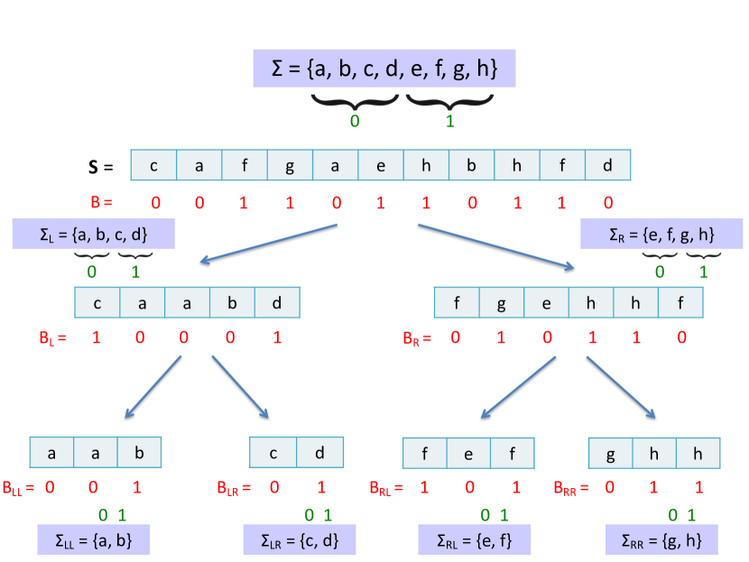
Figure 1: Example of a wavelet tree on the sequence $\operatorname{\sf S}=\texttt{cafgaehbhfd}$ and where $\sigma=8$ and the alphabet is $\Sigma=\{\texttt{a},\texttt{b},\texttt{c},\texttt{d},\texttt{e},\texttt{f},\texttt{g},\texttt{h}\}$. The root contains the entire sequence as well as a bitstring indicating whether the symbol comes from the left or the right half of $\Sigma$. The two children $L$ and $R$ of the root contain the characters in the left and right half of $\Sigma$, respectively. The bitstring for the left (right) child $B_{L}$ ($B_{R}$) is constructed by checking if the character comes from the left half or the right half of $\Sigma_{L}$ ($\Sigma_{R}$). The leaves each represent an alphabet of size $2$.

Each node in the wavelet tree stores a succinct rank/select structure on its bitstring (whose size is sub-linear in the bitstring length) to allow for constant-work rank and select queries. The bitstrings and the rank/select structures together take $n\lceil\log\sigma\rceil+o(n\log\sigma)$ bits of space. The wavelet tree topology requires $O(\sigma\log n)$ bits to store pointers, but this can be removed by modifying how the queries are performed [19, 5].

Our algorithms use prefix sum as a parallel primitive [27]. Prefix sum takes as input an array $X$ of length $n$, an associative binary operator $\oplus$, and an identity element $\bot$ such that $\bot\oplus x=x$ for any $x$, and returns the array $(\bot,\bot\oplus X[0],\bot\oplus X[0]\oplus X[1],\ldots,\bot\oplus X[0]\oplus X[1]\oplus\ldots\oplus X[n-2])$, as well as the overall sum $\bot\oplus X[0]\oplus X[1]\oplus\ldots\oplus X[n-1]$. Assuming that $\oplus$ takes constant work, prefix sum can be implemented in $O(n)$ work and $O(\log n)$ depth [27]. Unless specified otherwise, we will use $\oplus$ to be the addition operator on integers.

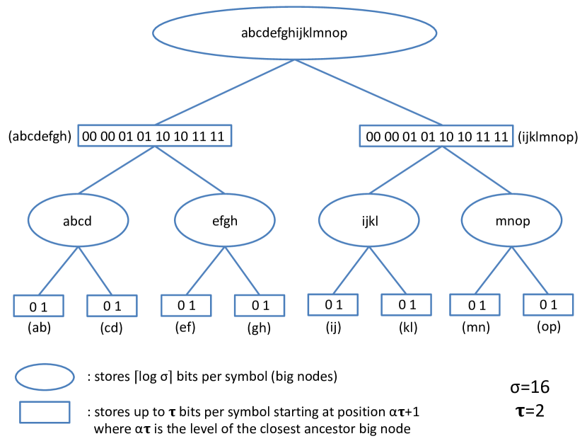
Figure 2: Example of the two types of nodes in the algorithm of Babenko et al. [1] for $\tau=2$ and $\sigma=16$. The alphabet is $\Sigma=\{\texttt{a},\texttt{b},\texttt{c},\texttt{d},\texttt{e},\texttt{f},\texttt{g},\texttt{h},\texttt{i},\texttt{j},\texttt{k},\texttt{l},\texttt{m},\texttt{n},\texttt{o},\texttt{p}\}$ and sequence is $\operatorname{\sf S}=\texttt{abcdefghijklmnop}$. The ovals correspond to big nodes, which store $\lceil\log\sigma\rceil=4$ bits per symbol. The rectangles correspond to the other nodes, which store up to $\tau=2$ bits per symbol in short lists (the symbols they represent are shown in parentheses next to the node). The bitstrings per node are not shown.

3 Review of the $O(n\lceil\log\sigma/\sqrt{\log n}\rceil)$ Work Sequential Algorithm

We first review how the $O(n\lceil\log\sigma/\sqrt{\log n}\rceil)$ work sequential wavelet tree construction algorithm from [1] works, as we will be parallelizing this algorithm. A similar sequential algorithm was independently described in [21]. Figure 2 illustrates the two types of nodes in the algorithm. The basic data structure used is a packed list, which stores $N$ $b$-bit integers using $\lceil Nb/\log n\rceil$ words. It supports appending a length $N$ list in $O(\lceil Nb/\log n\rceil)$ work and splitting a list into smaller lists of at most length $k$ in $O(\lceil Nb/\log n\rceil+N/k)$ work. These operations can be implemented using bit-shifts and copying. In this wavelet tree algorithm, a big node is defined to be a node at a level that is a multiple of $\tau$, where $\tau$ is a parameter to be chosen. A big node stores the symbols that it represents in $\operatorname{\sf S}$, using $\lceil\log\sigma\rceil$ bits per symbol as in the standard representation. Big nodes can be computed recursively as follows. The root is a big node storing $\operatorname{\sf S}$. Assume that the sub-sequences for the big nodes at level $\alpha\tau$ are already computed. Then to compute the symbols in the big nodes at level $(\alpha+1)\tau$, the big nodes at level $\alpha\tau$ look at the $\tau$ bits starting at position $\alpha\tau$ in the binary representation of each symbol to determine which of its descendant big nodes at level $(\alpha+1)\tau$ to place the symbol at (there are $2^{\tau}$ such descendants). Therefore, computation for big nodes requires $O(n\lceil\log\sigma/\tau\rceil)$ work overall.

Nodes at all other levels of the tree only need to store at most $\tau$ bits per symbol (the $\tau$ bits starting at position $\alpha\tau+1$, where $\alpha\tau$ is the level of its nearest big node ancestor) because there are only $\tau$ levels between two big node levels. These nodes use short lists to store $\tau$-bit integers containing the $\tau$ relevant bits of the symbols they represent. These are stored as packed lists. Computing the bitstring values and short lists is done recursively. The short lists of the children of a big node can be computed by extracting the relevant bits from the symbols of the big nodes in $O(n\lceil\log\sigma/\tau\rceil)$ work across all big nodes. Given a short list of a node, computing its own bitstring values and the short lists of its children is done via table lookup. For all packed lists $L$ of at most $\log n/(2\tau)$ $\tau$-bit integers, the bitstring value, and the packed lists $L_{0}$ and $L_{1}$ consisting of the symbols of $L$ whose $t$’th most significant bit is $0$ or $1$, respectively, are pre-computed for all $t\in[0,\tau-1]$. Pre-computing this table involves evaluating all $O(2^{\log n/2})$ $\tau$-bit integer sequences of length at most $\log n/(2\tau)$ for each value of $t$. This can be done in $O(n)$ work. Each node splits its short list into blocks of length at most $\log n/(2\tau)$, performs table lookups for each block, and then appends the resulting bitstring values together, $L_{0}$’s together, and $L_{1}$’s together. The bitstring values are stored in the bitstring associated with the current node, and $L_{0}$ and $L_{1}$ are passed to its children. For a node with a short list of length $N$, the total work required is $O(N\tau/\log n)$ as the splitting and merging can be done in $O(N\tau/\log n)$ work overall and table lookups in constant work per block. The sum of the lengths of all short lists is $O(n\log\sigma)$, and so the total work required for this computation is $O(n\lceil\log\sigma(\tau/\log n)\rceil)$.

The overall work is $O(n\lceil\log\sigma/\tau\rceil+n\lceil\log\sigma(\tau/\log n)\rceil)$ and choosing $\tau=\sqrt{\log n}$ minimizes the work, giving a bound of $O(n\lceil\log\sigma/\sqrt{\log n}\rceil)$. By constructing the tree level-by-level (i.e., interleaving big node computation with levels in between big nodes), at any time the algorithm only has to store the symbols for the big nodes at one level and short lists at one level, and so the peak space usage of the algorithm is $O(n\log\sigma)$ bits.

4 Parallel Wavelet Tree Algorithms

This section first describes how to parallelize the algorithm of Babenko et al. [1], which we reviewed in Section 3. Then we present a simple domain-decomposition based parallel construction algorithm that is work-efficient and whose parallelism depends linearly on $\sigma$, and so has low depth for small alphabets.

4.1 Parallelizing the algorithm of Babenko et al. [1]

The nodes in our parallel algorithm are classified the same way as in the sequential algorithm (see Figure 2). The sub-sequences for the big nodes can be computed level-by-level using parallel integer sorting. In particular, given the correct sub-sequence $\operatorname{\sf S}^{\prime}$ for a big node at level $\alpha\tau$, we compute the sub-sequences for its big node descendants at level $(\alpha+1)\tau$ by performing an integer sort on $\operatorname{\sf S}^{\prime}$, where the key for the sort is the value of the (up to) $\tau$ bits starting from the $\alpha\tau$’th highest bit of the symbol.

The parallel integer sort that we use is required to be stable since we need to keep the relative ordering among the characters in each descendant node. Unfortunately the only known method for stable parallel integer sorting in linear work and polylogarithmic depth [24] requires the range of the keys of the values being sorted to be polylogarithmic, which does not hold for the value of $\tau$ that we will choose. Instead we can either use an algorithm that is not work-efficient, requiring $O(n\log\log n)$ work and $O(\log n)$ depth [25, 2], or use a work-efficient algorithm with $O(n/\epsilon)$ work and $O(n^{\epsilon}/\epsilon)$ depth for a constant $0<\epsilon<1$ [27]. This gives an overall complexity for constructing big nodes of either (a) $O(n\log\log n\lceil\log\sigma/\tau\rceil)$ work and $O(\log n\lceil\log\sigma/\tau\rceil)$ depth or (b) $O((n/\epsilon)\lceil\log\sigma/\tau\rceil)$ work and $O((n^{\epsilon}/\epsilon)\lceil\log\sigma/\tau\rceil)$ depth for constructing the big nodes.

The lookup table for computing short lists can be pre-computed by evaluating all $O(2^{\log n/2})$ $\tau$-bit integer sequences of length at most $\log n/(2\tau)$ for each $t\in[0,\tau-1]$ in parallel, and storing the answer for each in a unique location. For example, this can be done using a three-level table, with the first level indexed by sequence length, second level by $t$, and third level by the value of the sequence as an integer. The result for each sequence and value of $t$ is evaluated sequentially. Overall, this requires $O(\log n)$ depth and $o(n)$ work.

Computing short lists for children of a big node can be done in linear work and $O(\log n)$ depth by extracting the relevant bits from the symbols in the big node, performing prefix sums to get the appropriate offsets, and copying the $\tau$ bits of a symbol into the appropriate location in an array of the appropriate child in parallel. Groups of $\tau$-bit integers that together form a word are then packed together and copied into one entry of the short list for the corresponding child in parallel. The bitstrings of the children of a big node can be computed in linear work and $O(\log n)$ depth simply by extracting the relevant bit from the symbols and packing them together. Computing short lists of other nodes requires merging and splitting packed lists. For each short list, we split it into chunks containing at most $\log n/(2\tau)$ $\tau$-bit integers by copying the relevant bits of each chunk into its own word in constant depth. The algorithm performs a table lookup for each chunk to obtain the parts of the packed lists $L_{0}$ and $L_{1}$ that the chunk contributes to as well as the part of the bitstring associated with the chunk. All table lookups are done in parallel in constant depth. We then merge together the results to form each of $L_{0}$, $L_{1}$, and the bitstring for the node. To merge the results of one of the lists together, we compute the length (in bits) of the result associated with each chunk, perform a prefix sum to determine the total length (in bits) and also the offset for each result in a new array, and allocate a new array of the desired length. We then identify the groups of chunks that will copy into the same word, again using prefix sums (some chunks will copy into two words, but this only increases the work by a constant factor). Then, in parallel, all groups merge their chunks sequentially using the packed list operations described in Section 3 and then copy their word into the new array at the appropriate offset. There are a total of $\lceil 2N\tau/\log n\rceil$ chunks if the short list contains $N$ integers, each of which generates a partial result for $L_{0}$, $L_{1}$, and the bitstring, and so the prefix sum and copying takes $O(N\tau/\log n)$ work and $O(\log n)$ depth (there is a constant-factor overhead due to some chunks not being full, however the complexity is not affected). The overall work for computing the short lists is $O(n\lceil\log\sigma(\tau/\log n)\rceil)$ as in the sequential algorithm. The depth is $O(\log n\log\sigma)$ as there are $\log\sigma$ levels, each requiring $O(\log n)$ depth.

To minimize the overall work we set $\tau=\sqrt{\log n\log\log n}$ when using the $O(n\log\log n)$ work integer sort and $\tau=\sqrt{\log n}$ when using the $O(n/\epsilon)$ work integer sort. Assuming that constructing the rank and select data structures per node can be done in the same bounds, which we describe in Section 5, we obtain the following theorem:

Theorem 4.1.

Wavelet tree construction can be performed in $O(n\log\log n\lceil\log\sigma/\allowbreak\sqrt{\log n\log\log n}\rceil)$ work and $O(\log n\log\sigma)$ depth (using randomization or super-linear space) or $O((n/\epsilon)\lceil\log\sigma/\sqrt{\log n}\rceil)$ work and $O((n^{\epsilon}/\epsilon)\lceil\log\sigma/\sqrt{\log n}\rceil)$ depth for a constant $0<\epsilon<1$.

Note that both parallel algorithms described above improve upon the $O(n\log\sigma)$ work complexity of the algorithms described in [26, 17]. Our algorithm either has polylogarithmic depth but does not achieve the $O(n\lceil\log\sigma/\sqrt{\log n}\rceil)$ work bound of the best sequential algorithm, or is work-efficient with sub-linear (but not polylogarithmic) depth. However, as long as the number of processors is sub-linear, the second algorithm can make full use of all of the available processors (recall Brent’s scheduling theorem and the definition of parallelism from Section 2). Improving parallel integer sorting algorithms would immediately improve the complexity of the wavelet tree algorithms.

We now analyze the working space of the algorithm. We also compute the tree level-by-level as in the sequential algorithm. We require $O(n\log n)$ bits of working space for the integer sort (assuming that we use [27] or [25]). The prefix sums and packing operations also require $O(n\log n)$ bits of working space. Finally, the lookup table contains $o(n)$ entries and therefore uses $o(n\log n)$ bits. Overall, our algorithm requires $O(n\log n)$ bits of working space.

4.2 Domain-decomposition approach

Another way to construct the wavelet tree in parallel is to use a domain-decomposition approach as done in [12, 17]. For a parameter $K$, this approach first splits the input sequence into $K$ equal-sized sub-sequences, constructs the wavelet tree (without rank/select structures) across all sub-sequences in parallel using a sequential algorithm for each, and then merges the bitstrings on the nodes of the $K$ trees together. An illustration of the domain-decomposition approach is shown in Figure 3. Constructing the tree for each sub-sequence can be done by using an $O(n\lceil\log\sigma/\sqrt{\log n}\rceil)$ work sequential algorithm [21, 1] in a black-box fashion (where the alphabet size for each sub-sequence is treated as the same as the alphabet size of the entire sequence). The overall work for this step is $O(n\lceil\log\sigma/\sqrt{\log n}\rceil)$ and the depth is $O((n/K)\lceil\log\sigma/\sqrt{\log n}\rceil)$.

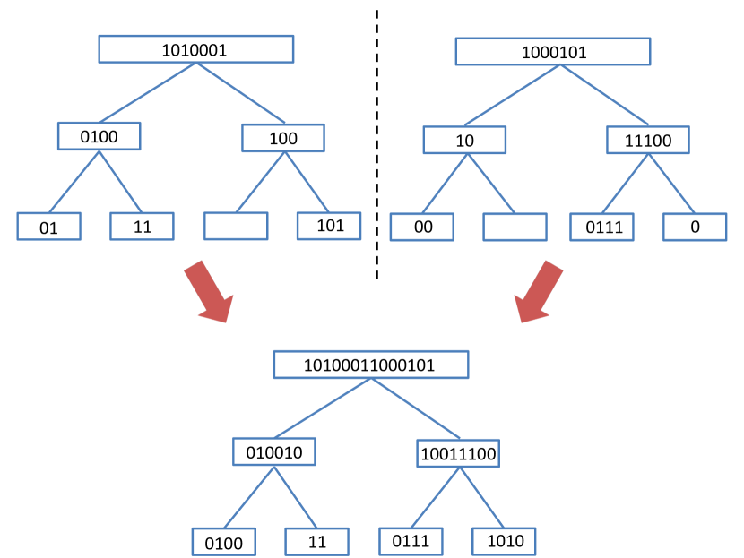
Figure 3: An illustration of the domain-decomposition approach where $K=2$. The sequence is split in half, and the wavelet trees, including bitstrings per node, are generated independently for each half (top). The bitstrings are then merged together for each node to obtain the final wavelet tree (bottom).

To merge together the bitstrings, we first form the wavelet tree structure (without bitstrings on nodes), which takes $O(\sigma)$ work and $O(1)$ depth. Following the idea described in [12, 17], for each node in the final tree structure, we then perform a prefix sum across the lengths of the bitstrings on the corresponding nodes in the $K$ sub-problems (the length is $0$ if the node does not exist) taking $O(K)$ work and $O(\log K)$ depth. This gives the length of the bitstring on the node in the final tree as well as an appropriate offset into the bitstring for each sub-problem. Then each sub-sequence copies its bitstring into the bitstring of the node in the final tree in parallel at word granularity. The words where multiple sub-sequences can copy into in parallel are marked beforehand to avoid conflicts and handled specially (these “boundary” words can be identified by looking at the offsets of the $O(\sigma K)$ nodes, and there can be at most $O(\sigma K)$ of them). Summed over all nodes in the final tree, the prefix sums take $O(\sigma K)$ work and $O(\log K)$ depth (the $\sigma$ different prefix sums can be done independently in parallel). Excluding the special words, the copying takes $O(n\log\sigma/\log n)$ work and $O(1)$ depth in total (the $\log n$ in the denominator of the work is because we are copying at word granularity). The special words can all be computed in parallel, taking $O(\sigma K)$ work and $O(\log K)$ depth by concatenating the up to $K$ bitstrings for each special word in a binary fashion. This gives the following theorem:

Theorem 4.2.

A wavelet tree can be constructed in $O(\sigma K+n\lceil\log\sigma/\sqrt{\log n}\rceil)$ work and $O((n/K)\lceil\log\sigma/\sqrt{\log n}\rceil+\log K)$ depth for any integer $K\geq 1$.

The domain-decomposition algorithm is work-efficient if $K=O((n/\sigma)\lceil\log\sigma/\sqrt{\log n}\rceil)$. Setting $K=\Theta((n/\sigma)\lceil\log\sigma/\sqrt{\log n}\rceil)$ gives the maximum parallelism while achieving work-efficiency, and gives a depth of $O(\sigma+\log n)$. Thus this algorithm has good parallelism for small $\sigma$, and achieves lower work than the domain-decomposition algorithm in [12, 16, 17].

The space required by the sequential algorithm across all sub-sequences is $O(n\log\sigma)$ bits. The domain-decomposition algorithm also requires $O(\sigma K\log n)$ bits of working space to represent the nodes of the trees of the sub-sequences and for the prefix sums. By setting $K=\Theta((n/\sigma)\log\sigma/\log n)$, the space usage does not asymptotically exceed the size of the final output of $O(n\log\sigma)$ bits, the work is $O(n\lceil\log\sigma/\sqrt{\log n}\rceil)$ and the depth is $O(\sigma\log n)$.

We can use a parallel algorithm to solve each of the $K$ sub-problems to improve the depth. In particular, if we plug in the $O((n/\epsilon)\lceil\log\sigma/\sqrt{\log n}\rceil)$ work and $O((n^{\epsilon}/\epsilon)\lceil\log\sigma/\sqrt{\log n}\rceil)$ depth algorithm from Section 4.1 into our domain-decomposition algorithm, we obtain the following theorem.

Theorem 4.3.

A wavelet tree can be constructed in $O(\sigma K+(n/\epsilon)\lceil\log\sigma/\sqrt{\log n}\rceil)$ work and $O(((n/K)^{\epsilon}/\epsilon)\lceil\log\sigma/\sqrt{\log n}\rceil+\log K)$ depth for any integer $1\leq K\leq n/\sigma$ and a constant $0<\epsilon<1$.

The upper bound on $K$ is due to the fact that integer sort takes linear work in both the sub-problem size as well as the range of keys being sorted. The range of keys being sorted is $O(\sigma)$, and so we need each sub-problem size to be $\Omega(\sigma)$ to amortize the work to the subproblem size and maintain work-efficiency. By setting $K=\Theta(n/\sigma)$, we obtain an algorithm with $O((n/\epsilon)\lceil\log\sigma/\sqrt{\log n}\rceil)$ work and $O((\sigma^{\epsilon}/\epsilon)\lceil\log\sigma/\sqrt{\log n}\rceil+\log n)$ depth. The working space is $O(n\log n)$ bits, due to the use of parallel integer sort.

4.3 Variants

This section describes how ideas from our binary wavelet tree construction algorithm from Section 4.1 can be used to construct variants of wavelet trees.

Arbitrarily-shaped binary trees. Our algorithm from Section 4.1 can be extended to binary trees of other shapes (e.g., Huffman-shaped wavelet trees [10]) if the tree structure can be computed efficiently and is of height $O(\log n)$. In particular, the algorithm needs a codeword for each symbol determined by the path from the root to the node representing the symbol in the tree. The codeword is a bitstring, where the $i$’th most significant bit is $0$ if the $(i+1)$’st node in the path is a left child of the $i$’th node in the path, and is $1$ otherwise. We define $h$ to be the height of the tree. We assume a lookup table storing a mapping from codeword to symbol. Since the codewords are of length $O(\log n)$, we can access the codeword in constant-work, and construct the lookup table in $O(\sigma)$ work and $O(\log n)$ depth. (We note that codewords for a Huffman-shaped wavelet tree can be generated in $O(n)$ work and $O(\sigma+\log n)$ depth [7, 26].)

To construct the tree, we first convert the symbols to their codewords. The algorithm proceeds as before, where big nodes are constructed every $\tau$’th level in the tree by using integer sorting on $\tau$ bits. Some of the combinations of the bits may not correspond to a symbol (which can be determined using the lookup table), and no big nodes are generated for those combinations. The complexity per level is equal to the complexity of integer sorting, and summing across all $h/\tau$ levels gives the following bounds for constructing big nodes: (a) $O(n\sqrt{\log\log n}\lceil h/\sqrt{\log n}\rceil)$ work and $O(\log n\lceil h/\sqrt{\log n\log\log n}\rceil)$ depth (by setting $\tau=\sqrt{\log n\log\log n}$) or (b) $O((n/\epsilon)\lceil h/\sqrt{\log n}\rceil)$ work and $O((n^{\epsilon}/\epsilon)\lceil h/\sqrt{\log n}\rceil)$ depth for $0<\epsilon<1$ (by setting $\tau=\sqrt{\log n}$). The remaining nodes that exist (which again can be checked using the lookup table) are computed using short lists as before, and the overall work for these nodes is $O(n\lceil h(\tau/\log n)\rceil)$ and depth is $O(h\log n)$. This gives the following theorem, whose work bound improves upon the parallel construction described in [26]:

Theorem 4.4.

Given codewords for the symbols, a binary wavelet tree of height $h=O(\log n)$ can be constructed in $O(n\log\log n\lceil h/\sqrt{\log n\log\log n}\rceil)$ work and $O(h\log n)$ depth or $O((n/\epsilon)\lceil h/\sqrt{\log n}\rceil)$ work and $O((n^{\epsilon}/\epsilon)\lceil h/\sqrt{\log n}\rceil)$ depth for a constant $0<\epsilon<1$.

The working space of the algorithm can be bounded by $O(n\log n)$ bits, as in Section 4.1.

Multiary wavelet trees. We now describe how to extend the algorithm to construct multiary wavelet trees [8] of degree $d=O(\log^{1/3-\delta}n)$, where $\delta>0$ and $d$ is a power of two. Each node now has $d$ children and the sequence that a node stores contains values in $[0,\ldots,d-1]$ instead of being binary as in the standard wavelet tree. We describe the algorithm for balanced trees but the ideas also apply to trees of arbitrary shapes as long as the codewords are provided as input. Similar to the approach of [21] we generate the full binary tree, but only keep sequences for the nodes at levels $\beta\log d$ in the full binary tree for $\beta=[0,\ldots,\log\sigma/\log d)$. Each node with a sequence that is kept belongs to the multiary wavelet tree, and if it is at level $\beta\log d$ in the binary tree, its $d$ children are at level $(\beta+1)\log d$ in the binary tree. With an appropriate numbering scheme (i.e., the children of node $i$ are stored at locations $2i+1$ and $2i+2$), the $d$ children of a node can be identified in $O(d)$ work and $O(1)$ depth, contributing $O(\sigma)$ work and $O(1)$ depth overall. Each node belonging to the multiary wavelet tree stores a sequence of $\log d$-bit integers, which can be computed by extracting the appropriate $\log d$ bits from its sequence of symbols. The bounds from Theorem 4.1 then apply, giving the following theorem which improves upon the work of the parallel algorithm for multiary wavelet trees from [26].

Theorem 4.5.

A multiary wavelet tree of degree $d=O(\log^{1/3-\delta}n)$ where $\delta>0$ and $d$ is a power of two can be constructed in $O(n\log\log n\lceil\log\sigma/\sqrt{\log n\log\log n}\rceil)$ work and $O(\log n\log\sigma)$ depth or $O((n/\epsilon)\lceil\log\sigma/\sqrt{\log n}\rceil)$ work and $O((n^{\epsilon}/\epsilon)$ $\lceil\log\sigma/\sqrt{\log n}\rceil)$ depth for $0<\epsilon<1$.

As in Section 4.1, the working space of the algorithm can be bounded by $O(n\log n)$ bits. We note that each node of a multiary wavelet tree requires storing a generalized rank and select structure on its sequence of $\log d$-bit integers, and we describe how to construct the structures within the bounds of Theorem 4.5 in Section 5.2.

Wavelet matrix. The wavelet matrix [6] is a variant of the wavelet tree where for level $l$, all symbols with a $0$ as their $l$’th highest bit are represented on the left side of the level’s sequence and all symbols with a $1$ as their $l$’th highest bit are represented on the right side. The relative ordering among the symbols from the previous level is preserved. Each level also contains an integer indicating the number of $0$’s per level. The wavelet matrix has $O(\log\sigma)$ levels. An $O(n\log\sigma)$ work, polylogarithmic depth parallel algorithm for constructing the wavelet matrix was described in [26]. In this section, we describe how to reduce the work complexity using similar ideas as described in Section 4.1.

We will process the bits of the symbols in chunks of $\tau$ bits and construct the matrix level-by-level. Every $\tau$’th level is treated specially, similar to the big nodes in Section 4.1. For an integer $\alpha$, to construct the sequence at level $(\alpha+1)\tau$ from level $\alpha\tau$ we perform an integer sort on the sequence at level $\alpha\tau$ using the reverse of the $\tau$ bits starting at the $\alpha\tau$’th position of the symbols. Constructing all special levels takes either (a) $O(n\log\log n\lceil\log\sigma/\tau\rceil)$ work and $O(\log n\lceil\log\sigma/\tau\rceil)$ depth or (b) $O((n/\epsilon)\lceil\log\sigma/\tau\rceil)$ work and $O((n^{\epsilon}/\epsilon)\lceil\log\sigma/\tau\rceil)$ depth.

Constructing levels $\alpha\tau+1$ to $(\alpha+1)\tau-1$ of the wavelet matrix will require only the (at most) $\tau$ bits starting at the $(\alpha\tau+1)$’th position of the symbols. We will create chunks of $\log n/(2\tau)$ $\tau$-bit integers, and use the packed list representation as in the wavelet tree algorithm. We use a lookup table storing all possible bitstrings of up to length $\log n/2$, which for each chunk and each bit position determines which symbols go to the left and which go to the right, as well as the bitstring, in $O(1)$ work. The lookup table can be computed in $O(\log n)$ depth and $o(n)$ work. Similar to the wavelet tree algorithm, each chunk can be split into two parts, the first that goes to the left side of the sequence and the second that goes to the right. Prefix sums and grouping of chunks are then used on the packed lists to create the bitstring for the current level as well as the sequence at the next level. On each level, this takes $O(n\lceil\tau/\log n\rceil)$ work and $O(\log n)$ depth. Summing over all levels gives $O(n\lceil\log\sigma(\tau/\log n)\rceil)$ work and $O(\log n\log\sigma)$ depth.

To compute the number of $0$’s in the bitstring for each level, we create a lookup table mapping all possible bitstrings of up to length $\log n/2$ to the number of $0$’s in the bitstring. This can be constructed in $O(\log n)$ depth and $o(n)$ work. Then we split each bitstring into chunks of length $\log n/2$, perform table lookup for each chunk, and perform a prefix sum on the $O(n/\log n)$ results. We do this level-by-level so the total work for prefix sums across all levels is $O(n\log\sigma/\log n)$ and span is $O(\log n\log\sigma)$.

Setting $\tau$ to either $\sqrt{\log n\log\log n}$ or $\sqrt{\log n}$ to minimize the total work gives the following theorem:

Theorem 4.6.

Wavelet matrix construction can be performed in $O(n\log\log n\lceil\log\sigma/\allowbreak\sqrt{\log n\log\log n}\rceil)$ work and $O(\log n\log\sigma)$ depth or $O((n/\epsilon)\lceil\log\sigma/\sqrt{\log n}\rceil)$ work and $O((n^{\epsilon}/\epsilon)\lceil\log\sigma/\sqrt{\log n}\rceil)$ depth for a constant $0<\epsilon<1$.

By constructing the matrix level-by-level, we can bound the working space by $O(n\log n)$ bits.

Similar to binary wavelet tree construction, we believe that a domain-decomposition approach can be used to improve the depth of the work-efficient algorithms for the variants described in this sub-section.

5 Improved Parallel Construction of Rank/Select Structures

Wavelet trees and matrices require each node to store a succinct rank and select structure on its bitstrings or sequences of $(\log d)$-bit values. We show how to construct these structures in parallel within the bounds of the construction algorithms described in Section 4.

5.1 Binary Sequences

We first describe the binary sequence case. The goal is to construct the rank/select structures on $n$ bits in $O(n/\log n)$ work to match the work bound of the sequential construction algorithms in [1]. The overall work for rank/select construction in a wavelet tree will therefore be $O(n\log\sigma/\log n)$, which is within the work bound of our parallel wavelet tree algorithms. We assume that the bit sequence is packed into $n/\log n$ words, which is provided by our wavelet tree algorithms from Section 4.

Rank. For rank queries, we use the structure of Jacobson [14]. We only store the rank of $0$ since the rank of $1$ can be derived from the rank of the $0$. The data structure divides the bit sequence into ranges of size $\log^{2}n$. It computes the rank for the last bit in each range. The ranges are further divided into sub-ranges of size $\log n$, where the rank of every $\log n$’th bit relative to the beginning of the range is stored. Inside a sub-range, the rank of a position relative to the beginning of the sub-range can be answered with at most two table lookups, where the table stores the answers to all queries of sequences of up to length $\log n/2$.

We initialize an array, $A_{0}$, of length $n/\log n$, and for each of the $n/\log n$ words, we count the number of $0$’s in the word and store them into its position in the appropriate array. Counting the number of $0$’s in a word can be done in $O(1)$ work using the same lookup table as for answering rank queries. Then we compute the prefix sum over $A_{0}$. Then, every $\log n$’th entry in $A_{0}$ gives the rank for the last position in each range. The results for the sub-ranges are computed by taking each remaining entries in $A_{0}$, and subtracting the rank stored for the closest range to the left. The prefix sums require $O(n/\log n)$ work and $O(\log n)$ depth. The lookup tables can be generated in parallel in $o(n/\log n)$ work and $O(\log n)$ depth. The results for the sub-ranges should be represented using $O(\log\log n)$ bits each, and groups of $O(\log n/\log\log n)$ entries can be packed into a word as a post-processing step in $O(n/\log n)$ work and $O(\log n)$ depth.

Select. For select queries, we use Clark’s select structure [4], which uses $O(n/\log\log n)$ extra bits for an input of length $n$. We describe the case for querying the location of $1$ bits, and the case for querying $0$ bits is analogous. Clark’s data structure stores the location of every $\log n\log\log n$’th $1$ bit, which defines ranges. For a range of length $r$ between the locations, if $r\geq\log^{2}n(\log\log n)^{2}$, then the answers to all of the possible select queries in the range are directly stored. Otherwise, the location of every $\log r\log\log n$’th $1$ bit is stored, which defines sub-ranges. For a sub-range of length $r^{\prime}$, if $r^{\prime}\geq\log{r^{\prime}}\log r(\log\log n)^{2}$ then answers are stored directly relative to the start of the sub-range using $O(\log\log n)$ bits each. Queries that fall into all other sub-ranges are answered via a lookup table that stores all answers for bitstrings of length $r^{\prime}=O((\log\log n)^{4})$.

To construct the select structure, we count the number of $1$’s in each of the $2n/\log n$ half-words using table lookup, and perform a prefix sum over the $2n/\log n$ results. We can now identify all of the half-words that contain the location of a $k\log n\log\log n$’th $1$ bit, for any integer $k$. Using table lookup we can find the location of the $j$’th occurrence (for a value of $j$ determined by the prefix sum) of a $1$ bit in a half-word in $O(1)$ work, which we then offset by the starting location of the half-word. This can be done in $O(n/\log n)$ work and $O(\log n)$ depth. This also allows us to determine the range lengths. For the ranges of length at least $\log^{2}n(\log\log n)^{2}$, we scan through the half-words in the range and store the location of every $1$ bit. The location of all $1$ bits within a half-word can be determined in $O(x)$ work and $O(1)$ depth via table lookup, where $x$ is the number of $1$’s in the half-word (the $O(x)$ term comes from having to output the $x$ locations). The locations within the half-word are then offset by the starting location of the half-word, again taking $O(x)$ work and $O(1)$ depth. Scanning the half-words takes $O(n/\log n)$ work and $O(\log n)$ depth. There are at most $n/(\log n\log\log n)$ locations of $1$ bits found this way, and we can store their locations in the appropriate range in $O(n/(\log n\log\log n))$ work and $O(1)$ depth using the result of the previous prefix sum and subtracting the offset of where its range begins.

For ranges of length less than $\log^{2}n(\log\log n)^{2}$, we perform a prefix sum over the half-words (as before, the count in a half-word is found via table lookup) in the range to identify which half-words have boundaries for sub-ranges, which takes $O(n/\log n)$ work and $O(\log n)$ depth overall. Directly generating the boundary locations and then packing them into words would require $O(n/(\log r\log\log n))$ work since there could be that many locations, and this is too much. Instead, for the half-words that have boundaries, we output all of the boundary locations (relative to the beginning of the range) in packed representation by using table lookup. The lookup table takes a half-word, a skip amount $s$, an offset $j$, and a length $r$ (these values are all bounded by the range length $\log^{2}n(\log\log n)^{2}$), and outputs the location offset by $j$ of every $s+k\log r\log\log n$’th $1$ bit for all $k$ in a packed representation. It can be constructed by considering all possible half-words, and all possible values of $s$, $j$, and $r$, in $o(n/\log n)$ work and $O(\log n)$ depth. There are at most $O(n/(\log r\log\log n))$ boundaries, and each takes $O(\log\log n)$ bits to store. We can output $O(\log n/\log\log n)$ boundaries in a word in constant work, and so outputting all of the boundaries takes $O(n/(\log r\log n))=O(n/\log n)$ work and $O(\log n)$ depth.

If answers in the sub-range need to be stored directly (i.e., the sub-range length $r^{\prime}$ is at least $\log{r^{\prime}}\log r(\log\log n)^{2}$), then as mentioned before we store the answers relative to the start of the sub-range using $O(\log\log n)$ bits each. We will generate the locations of all $1$ bits relative to the start of the range in each half-word by using table lookup, where the result is packed into groups of $O(\log n/\log\log n)$ relative locations. The lookup table also takes as input how much to offset each answer. The offsets can be computed via a prefix sum over the counts of $1$ bits in the half-words. The number of locations of $1$ bits output is at most $O(n/(\log\log n)^{2})$, and so the number of groups is at most $O(n/(\log n\log\log n))$. The last group in each half-word might not be fully packed but this only increases the number of groups by a constant factor. The offsets for storing the groups for each half-word can be pre-computed via prefix sums. The lookup table takes at most $\log^{2}n(\log\log n)^{2}$ possible offsets, and has $O(2^{\log n/2})$ entries per offset, so can be constructed in $o(n/\log n)$ work and $O(\log n)$ depth. The overall work for this step is thus $O(n/\log n)$ and the depth is $O(\log n)$. Finally, for the sub-ranges of length $r^{\prime}<\log{r^{\prime}}\log r(\log\log n)^{2}=O((\log\log n)^{4})$, the queries are answered via a lookup table that can be computed in $o(n/\log n)$ work and $O(\log n)$ depth.

For the select queries to work properly, all of the words inside each range and sub-range except the last should be fully packed, but this can be fixed with a post-processing step that generates an array of new words, and computes for each old word where it should copy its results in the new word using a prefix sum. In parallel, each new word is then constructed sequentially from the corresponding old words. There are a total of $O(n/\log n)$ words in total, so this takes $O(n/\log n)$ work and $O(\log n)$ depth.

We have the following theorem for constructing rank/select structures on binary sequences:

Theorem 5.1.

The rank and select structures for a binary sequence of length $n$ packed into $n/\log n$ words can be constructed in $O(n/\log n)$ work and $O(\log n)$ depth.

The prefix sums operate on inputs of size $O(n/\log n)$ and therefore take $O(n)$ bits of working space. The lookup tables used all contain $o(n/\log n)$ entries and take $o(n)$ bits of working space. Thus our algorithms use $O(n)$ bits of working space.

5.2 Generalized Rank and Select Structures

In this section, we show how to construct rank and select structures on sequences with alphabets $\sigma=O(\log^{1/3-\delta}n)$ for $\delta>0$ (this solution can also be used for binary sequences although the solution described in Section 5.1 is simpler). For a sequence of length $n$, Shun [26] describes how to construct the structures for $O(n)$ work and $O(\log n)$ depth. We show that the construction can be done in $O(n\log\sigma/\log n)$ work and $O(\log n)$ depth. While a work bound of $O(n/\sqrt{\log n})$ suffices for use in the multiary wavelet tree algorithm described in Section 4, our goal is to match the work of the sequential algorithms for constructing the generalized rank/select structures of [1]. We assume the input is packed into $n\log\sigma/\log n$ words.

Rank. For the rank structure, a query $\operatorname{\sf rank}_{\leq c}(S,i)$ returns the number of times a symbol less than or equal to $c$ appears from positions $0$ to $i$, which differs from the binary case. Thus, simply creating $\sigma$ copies of the binary rank structure, one for each character, will not suffice. We will instead use the generalized rank structure described in [1].

For every $\sigma\log^{2}n$’th symbol in the sequence, the generalized rank structure of [1] stores the $\sigma$ ranks of that symbol (there is one rank per character in the alphabet). These symbols define ranges in the sequence, and we will refer to them as range symbols. For each range, the $\sigma$ ranks of every $\log n/(3\log\sigma)$’th symbol relative to the beginning of the range are stored. These symbols define sub-ranges, which we refer to as sub-range symbols. Queries inside a sub-range are of length at most $\log n/(3\log\sigma)$ and can be answered in $O(1)$ work via table lookup. The table has $O(\sigma^{\log n/(3\log\sigma)}\log n/(3\log\sigma))$ entries per character, which sums to $o(n\log\sigma/\log n)$ overall, and thus can be constructed in $o(n\log\sigma/\log n)$ work and $O(\log n)$ depth using similar ideas as before.

We first describe how to compute the ranks of all sub-range symbols relative to the beginning of its range. The algorithm requires pre-computing two lookup tables. The first table takes as input a block of $\log n/(3\log\sigma)$ symbols and outputs the generalized ranks for the last symbol in the block relative to the beginning of the block in $O(1)$ work. The second table takes as input two sets of generalized ranks relative to the beginning of the range and outputs the sum of the generalized ranks in $O(1)$ work. Both tables can be constructed in $o(n\log\sigma/\log n)$ work and $O(\log n)$ depth. The algorithm first passes the $\log n/(3\log\sigma)$ symbols closest to the left of (and including) each sub-range symbol to the first table. The generalized ranks relative to the beginning of the range can now be computed in parallel using a prefix sum where the combining operator $\oplus$ is defined by the second lookup table. Note that the combining operation is associative, as required by prefix sum. Over all ranges, there are $3n\log\sigma/\log n$ symbols that we compute ranks for, and so the prefix sum takes $O(n\log\sigma/\log n)$ work and $O(\log n)$ depth. The results can be packed tightly into words using similar ideas as before.

To compute the generalized ranks for the range symbols, we first obtain the generalized ranks of the last symbol of each range relative to the beginning of the range. This can be obtained by summing the generalized ranks of the last sub-range symbol in the range with the ranks of the remaining symbols after it (relative to the last sub-range symbol) using the two lookup tables defined above. We then perform a prefix sum over these values to obtain the generalized ranks relative to the beginning of the sequence. When combining two entries, we can simply scan through all $\sigma$ characters (in parallel) and update their generalized ranks. Each combining operation takes $O(\sigma)$ work and $O(1)$ depth, and there are $O(n/(\sigma\log^{2}n))$ entries, giving a total complexity of $O(n/\log^{2}n)$ work and $O(\log n)$ depth. The generalized ranks for the range symbols can now be computed by looking at the ranks of the last symbol in the previous range and updating it with the value of the range symbol. The overall complexity for constructing the rank structure is $O(n\log\sigma/\log n)$ work and $O(\log n)$ depth.

Select. For the select structure, we could simply create $\sigma$ copies of the binary select structure in Section 5.1, one per character. However, the binary select structure that we use takes $O(n/\log\log n)$ bits of space, and so this will not be a succinct representation for large $\sigma$. We will therefore parallelize the construction of the generalized select structure described in [1]. It has been described how to do this in $O(n)$ work in [26], but to do this in $O(n\log\sigma/\log n)$ work to match the bound in [1] requires additional care.

We will have a separate select structure for each character but the structure is not the same as in the binary case. For a character $c$, the structure stores the location of every $\sigma\log^{2}n$’th occurrence of $c$, and these occurrences define ranges (call these occurrences range symbols). For each range, if the length is at least $\sigma^{2}\log^{4}n$ then we store the answers directly, and otherwise we store the locations for every $\sigma(\log\log n)^{2}$’th occurrence of $c$ relative to the start of the range, which define sub-ranges (call these occurrences sub-range symbols). For a sub-range, if the length is at least $\sigma^{3}(\log\log n)^{4}$, the answers are stored directly, and otherwise a lookup table is used to answer any query in the sub-range in $O(1)$ work. The table contains $O(2^{\sigma^{3}(\log\log n)^{4}}\sigma^{3}(\log\log n)^{4})=o(n\log\sigma/(\sigma\log n))$ entries since $\sigma=O(\log^{1/3-\delta}n)$ for $\delta>0$. Thus it can be constructed within the desired complexity bounds.

We will construct the select structures for all characters together. We first split the input sequence into chunks of $\log^{2}n/(3\log\sigma)$ symbols and compute the number of occurrences of each character inside a chunk. Each chunk is further split into groups of $\log n/(3\log\sigma)$ symbols each. We can output the number of occurrences of each character in a group using table lookup in $O(1)$ work. The table contains $O(2^{\log n/3})$ entries, and thus can be computed in $o(n\log\sigma/\log n)$ work and $O(\log n)$ depth. We can also use table lookup to add two sets of $\sigma$ counts together in $O(1)$ work. Each count has a maximum value of $\log^{2}n/(3\log\sigma)$ and thus any count requires $O(\log\log n)$ bits to represent. The number of possible inputs to this table is therefore $2^{O(2\sigma\log\log n)}=o(n\log\sigma/\log n)$ and so the table can be constructed within the desired bounds. To compute the number of occurrences of each character inside a chunk, we sum together the occurrences across the groups sequentially. This takes $O(\log n)$ depth since there are $\log n$ groups per chunk. The computation is parallelized across all chunks and the overall work performed is $O(n\log\sigma/\log n)$ and overall depth is $O(\log n)$.

Now we must find the range symbols. We perform a prefix sum over the answers computed above, where the associative combining operator is defined by a lookup table that takes the $\sigma$ counts from two chunks and outputs the $\sigma$ counts that correspond to the sum of the counts from the two input chunks. The counts here will be relative to the beginning of the sequence, and thus an output can take $O(\sigma\log n)$ bits to represent and $O(\sigma)$ work to output. There are $O(n\log\sigma/\log^{2}n)$ chunks, and thus the prefix sum takes $O(n\sigma\log\sigma/\log^{2}n)=O(n\log\sigma/\log n)$ work and $O(\log n)$ depth.

We now know the number of occurrences of each character in each chunk as well as from the beginning of the sequence up to that chunk. This allows us to identify which chunks the range symbols occur in for a given character, and we search in the associated groups in the chunk for the location of the range symbol. For each chunk, we scan over the groups sequentially updating the number of times we have seen a symbol so far via table lookup. Whenever we find a group that contains a range symbol, we use table lookup find the location of the $j$’th occurrence of a character inside the group in $O(1)$ work for an appropriate value of $j$. Thus, processing each chunk takes $O(\log n)$ work and depth. The lookup table can be constructed in $o(n\log\sigma/\log n)$ work and $O(\log n)$ depth. This process gives all of the range symbols for a single character. There are at most $n/(\sigma\log^{2}n)$ chunks that need to be checked per character, each one taking $O(\log n)$ work. Summed across all characters, the work is $O(n/\log n)$ and the depth is $O(\log n)$ (we can do this process for all characters and all chunks in parallel).

With this information, we can compute the lengths of the ranges between range symbols. For a given character $c$, for the ranges that are at least $\sigma^{2}\log^{4}n$ long, we store all of the locations of $c$. Finding these locations requires scanning the relevant chunks, which takes $O(n\log\sigma/\log n)$ work and $O(\log n)$ depth (each chunk is scanned sequentially). If we mark the relevant chunks for each character beforehand, one scan over all of the chunks suffices to obtain the information for all characters. In particular on each chunk, for each character, we mark the start and the end of the chunk that it should consider (with a special value if a character’s long ranges do not span the chunk). This information on each chunk requires $O(\sigma\log\log n)=o(\log n)$ bits and thus can be packed into a word and accessed in constant work. The scan over all chunks takes $O(n\log\sigma/\log n)$ work and $O(\log n)$ depth, and for each chunk we use a lookup table to find the locations of the relevant characters in each group. The lookup table takes as input a group as well as the information stored on the chunk, and outputs the locations of all of the relevant characters relative to the start of the group (each location is tagged with the corresponding character). The work of the query is proportional to the number of locations returned. The table has $2^{O(\sigma\log\log n)}\cdot O(2^{\log n/3})$ entries and can be constructed in $o(n\log\sigma/\log n)$ work and $O(\log n)$ depth. The number of locations returned is at most $n/(\sigma^{2}\log^{4}n)\cdot\sigma\log^{2}n=O(n/(\sigma\log^{2}n))$ per character. Summed over all characters gives $O(n/\log^{2}n)$ work for returning the answers to the queries. These locations are offset by the start of the associated group. Overall, this step takes $O(n\log\sigma/\log n)$ work and $O(\log n)$ depth. To store these locations, we can pre-allocate space for these long ranges and compute offsets using prefix sums within the desired work and depth bounds.

For ranges of length less than $\sigma^{2}\log^{4}n$, we compute the sub-range symbols. This process is mostly similar to how the range symbols were computed but since there can be up to $n/(\sigma(\log\log n)^{2})$ sub-range symbols per character, outputting their locations directly would take too much work. However, the locations only require $O(\log\log n)$ bits each so we can output $O(\log n/\log\log n)$ locations in a packed representation in constant work. We store on each chunk the start and the end of the chunk each character should consider for its short range. The lookup table takes as input a group, the information on the chunk (let $C$ be the set of characters to consider), a skip amount $s_{c}$ for each $c\in C$, and an offset $j$, and outputs the locations offset by $j$ of every $s_{c}+k\sigma(\log\log n)^{2}$’th occurrence of $c\in C$ in a group for all integers $k$. The offset $j$ is used to make the locations relative to the beginning of the sub-range. Both $s_{c}$ and $j$ are bounded by the range length, which is $\sigma^{2}\log^{4}n$. The output locations are tagged with the corresponding character and given in a packed representation ($O(\log n/\log\log n)$ locations per word). The total work for writing out the locations of sub-range symbols will then be $O(n/(\sigma(\log\log n)^{2}))\cdot\sigma\cdot\log\log n/\log n=o(n\log\sigma/\log n)$. The lookup table can be constructed in $o(n\log\sigma/\log n)$ work and $O(\log n)$ depth. The overall work is $O(n\log\sigma/\log n)$ and depth is $O(\log n)$.

To determine sub-ranges of length at least $\sigma^{3}(\log\log n)^{4}$, we first return all sub-range starting locations for all characters that satisfy this inside a group using a lookup table. The table will return the (packed) locations of the sub-ranges that satisfy this property. The information on each chunk with the start and the end of the chunk in a short range for each character is also passed to the lookup table. The table can then determine which subset of characters to output sub-range starting locations for inside a group. The number of entries in the table is $2^{O(\sigma\log\log n)}\cdot O(2^{\log n/3})$ and can be constructed within our complexity bounds. However, since sub-ranges can span multiple groups, we then use a prefix sum across all groups where the associative operator is a lookup table that combines two groups by keeping the latest location of each relevant character in the first group and earliest location of each relevant character in the second. It uses the information on the chunk to determine which characters are relevant, and for which part of the groups they are relevant. It also outputs any sub-range starting locations where the difference between the latest location in the first group and the earliest location in the second is at least $\sigma^{3}(\log\log n)^{4}$. This table has $2^{O(\sigma\log\log n)}\cdot O(2^{2\log n/3})$ entries and can again be constructed within the desired bounds. Without accounting for the cost of outputting the locations, the prefix sum across all groups takes $O(n\log\sigma/\log n)$ work and $O(\log n)$ depth. For each character, there are at most $n/(\sigma^{3}(\log\log n)^{4})$ sub-ranges requiring answers to be stored directly, each containing $\sigma(\log\log n)^{2}$ locations that require $O(\log\log n)$ bits each. By returning the locations in packed representation, the total work is $O(n/(\sigma^{3}(\log\log n)^{4}))\cdot\sigma(\log\log n)^{2}\cdot\sigma\cdot\log\log n/\log n=o(n\log\sigma/\log n)$. The work for outputting the intermediate results in the prefix sum is also proportional to this.

Finally, for the remaining sub-ranges we create a lookup table that takes a group and the information on a chunk, and outputs the position (relative to the beginning of the sub-range) of all relevant occurrences (tagged with the character) in a packed representation. Constructing this table can be done within the desired bounds.

Overall, constructing the generalized select structure takes $O(n\log\sigma/\log n)$ work and $O(\log n)$ depth. Combined with the algorithm for constructing the generalized rank structure, we have the following theorem:

Theorem 5.2.

For a sequence of length $n$ containing characters in $[0,\ldots,\sigma-1]$ packed into $n\log\sigma/\log n$ words, where $\sigma=O(\log^{1/3-\delta}n)$ for $\delta>0$, the corresponding generalized rank and select structures can be constructed in $O(n\log\sigma/\log n)$ work and $O(\log n)$ depth.

The algorithms use prefix sums on inputs of length $O(n\log\sigma/\log n)$ and therefore require $O(n\log\sigma)$ bits of working space. The lookup tables all contain $o(n\log\sigma/\log n)$ entries, therefore using $o(n\log\sigma)$ bits of working space.

6 Conclusion

We have described parallel algorithms for wavelet tree construction with improved work complexity. The ideas extend to constructing wavelet trees of arbitrary shape, multiary wavelet trees, as well as wavelet matrices. We also showed that the rank and select structures stored on the nodes of the wavelet tree can be constructed work-efficiently in parallel. An open problem is obtaining a parallel wavelet tree algorithm with $O(n\lceil\log\sigma/\sqrt{\log n}\rceil)$ work and polylogarithmic depth for any value of $\sigma$. We are also interested in improving the working space bound of some of our algorithms.

References

- [1] M. A. Babenko, P. Gawrychowski, T. Kociumaka, and T. A. Starikovskaya. Wavelet trees meet suffix trees. In ACM-SIAM Symposium on Discrete Algorithms (SODA), pages 572–591, 2015.
- [2] P. C. P. Bhatt, K. Diks, T. Hagerup, V. C. Prasad, T. Radzik, and S. Saxena. Improved deterministic parallel integer sorting. Information and Computation, 94(1):29–47, 1991.
- [3] R. P. Brent. The parallel evaluation of general arithmetic expressions. J. ACM, 21(2):201–206, 1974.
- [4] D. R. Clark. Compact pat trees. Ph.D. Thesis, University of Waterloo, 1996.
- [5] F. Claude and G. Navarro. Practical rank/select queries over arbitrary sequences. In String Processing and Information Retrieval (SPIRE), pages 176–187, 2008.
- [6] F. Claude and G. Navarro. The wavelet matrix. In String Processing and Information Retrieval (SPIRE), pages 167–179. 2012.
- [7] J. A. Edwards and U. Vishkin. Parallel algorithms for Burrows-Wheeler compression and decompression. Theor. Comput. Sci., 525:10–22, Mar. 2014.
- [8] P. Ferragina, G. Manzini, V. Mäkinen, and G. Navarro. Compressed representations of sequences and full-text indexes. ACM Trans. Algorithms, 3(2), May 2007.
- [9] J. Fischer, F. Kurpicz, and M. Löbel. Simple, fast and lightweight parallel wavelet tree construction. In Meeting on Algorithm Engineering and Experiments (ALENEX), pages 9–20, 2018.
- [10] L. Foschini, R. Grossi, A. Gupta, and J. S. Vitter. When indexing equals compression: Experiments with compressing suffix arrays and applications. ACM Trans. Algorithms, 2(4):611–639, Oct. 2006.
- [11] J. Fuentes-Sepulveda, E. Elejalde, L. Ferres, and D. Seco. Efficient wavelet tree construction and querying for multicore architectures. In Symposium on Experimental Algorithms (SEA), pages 150–161, 2014.
- [12] J. Fuentes-Sepulveda, E. Elejalde, L. Ferres, and D. Seco. Parallel construction of wavelet trees on multicore architectures. Knowledge and Information Systems, 51(3):1–24, Jun 2017.
- [13] R. Grossi, A. Gupta, and J. S. Vitter. High-order entropy-compressed text indexes. In ACM Symposium on Discrete Algorithms (SODA), pages 841–850, 2003.
- [14] G. J. Jacobson. Succinct static data structures. Ph.D. Thesis, Carnegie Mellon University, 1988.
- [15] Y. Kaneta. Fast wavelet tree construction in practice. In String Processing and Information Retrieval (SPIRE), pages 218–232, 2018.
- [16] J. Labeit. Parallel lightweight wavelet tree, suffix array and FM-index construction. B.S. Thesis, Karlsruhe Institute of Technology, 2015.
- [17] J. Labeit, J. Shun, and G. E. Blelloch. Parallel lightweight wavelet tree, suffix array and FM-index construction. Journal of Discrete Algorithms, 43:2–17, 2017.
- [18] V. Mäkinen, D. Belazzougui, F. Cunial, and A. I. Tomescu. Genome-Scale Algorithm Design: Biological Sequence Analysis in the Era of High-Throughput Sequencing. Cambridge University Press, 2015.
- [19] V. Makinen and G. Navarro. Rank and select revisited and extended. Theor. Comput. Sci., 387(3):332–347, 2007.
- [20] C. Makris. Wavelet trees: A survey. Comput. Sci. Inf. Syst., 9(2):585–625, 2012.
- [21] J. I. Munro, Y. Nekrich, and J. S. Vitter. Fast construction of wavelet trees. In String Processing and Information Retrieval (SPIRE), pages 101–110, 2014.
- [22] G. Navarro. Wavelet trees for all. In Combinatorial Pattern Matching (CPM), pages 2–26. 2012.
- [23] G. Navarro. Compact Data Structures: A Practical Approach. Cambridge University Press, 1st edition, 2016.
- [24] S. Rajasekaran and J. H. Reif. Optimal and sublogarithmic time randomized parallel sorting algorithms. SIAM J. Comput., 18(3):594–607, 1989.
- [25] R. Raman. The power of collision: Randomized parallel algorithms for chaining and integer sorting. In Foundations of Software Technology and Theoretical Computer Science (FSTTCS), pages 161–175, 1990.
- [26] J. Shun. Parallel wavelet tree construction. In IEEE Data Compression Conference (DCC), pages 63–72, 2015.
- [27] U. Vishkin. Thinking in parallel: Some basic data-parallel algorithms and techniques, 2010.