On the free-precession candidate PSR B1828-11: Evidence for increasing deformation

Abstract

We observe that the periodic variations in spin-down rate and beam-width of the radio pulsar PSR B1828-11 are getting faster. In the context of a free precession model, this corresponds to a decrease in the precession period $P_{\mathrm{fp}}$. We investigate how a precession model can account for such a decrease in $P_{\mathrm{fp}}$, in terms of an increase over time in the absolute biaxial deformation ($|\epsilon_{\mathrm{p}}|{\sim}10^{-8}$) of this pulsar. We perform a Bayesian model comparison against the ‘base’ precession model (with constant $\epsilon_{\mathrm{p}}$) developed in Ashton et al. (2016), and we obtain decisive odds in favour of a time-varying deformation. We study two types of time-variation: (i) a linear drift with a posterior estimate of $\dot{\epsilon}_{\mathrm{p}}{\sim}10^{-18}\,\mathrm{s}^{-1}$ and odds of $10^{75}$ compared to the base-model, and (ii) $N$ discrete positive jumps in $\epsilon_{\mathrm{p}}$ with very similar odds to the linear $\epsilon_{\mathrm{p}}$-drift model. The physical mechanism explaining this behaviour is unclear, but the observation could provide a crucial probe of the interior physics of neutron stars. We also place an upper bound on the rate at which the precessional motion is damped, and translate this into a bound on a dissipative mutual friction-type coupling between the star’s crust and core.

1 Introduction

The ${\sim}500$ day periodicity observed in the timing properties and pulse profile of PSR B1828-11 provides a unique opportunity to test neutron star physics. The first model, proposed by Bailes et al. (1993), consisted of a system of planets orbiting the pulsar. This model later lost favour, after Stairs et al. (2000) observed correlated modulation in the timing properties and beam-shape (the ratio of the heights of two fitted integrated pulse profiles). As such, a planetary model would require at least two orbiting planets with orbital frequencies that differ by a factor of 2 (see for example Beaugé et al. (2003)), while both interact with the magnetosphere over distances comparable to the Earth’s orbit.

Instead, Stairs et al. (2000) proposed that the star was undergoing free precession, corresponding to a star that is deformed, with its spin-vector and angular momentum vectors misaligned. Subsequent modelling by Jones & Andersson (2001), Link & Epstein (2001) and Akgün et al. (2006) refined the precessional description, examining how the precessional motion served to amplify the modulations in spin-down rate, providing some quantitative detail to the precessional interpretation.

The existence of long period free precession has implications for the interaction between the superfluid, superconducting and ‘normal’ parts of the star. As shown by Shaham (1977), a pinned superfluid, as typically invoked to explain pulsar glitches, would result in a rather short free precession period, so that the observed long period can be used to place upper limits on the amount of pinned vorticity in PSR B1828-11; see Jones & Andersson (2001), Link & Epstein (2001) and Link & Cutler (2002). Furthermore, the interaction between neutron vortices and magnetic flux tubes in the stellar core is likely to be highly dissipative, which led to Link (2003) drawing the interesting conclusion that the persistence of the free precession required that neutron superfluidity and proton type II superconductivity coexist nowhere in the star, or else that the superconductivity is of type I. Additionally, Wasserman (2003) has argued that a sufficiently strong magnetic deformation of the stellar structure might force the star to undergo free precession. The issue of whether or not PSR B1828-11 really is precessing is therefore very important, in terms of its microphysical implications.

Motivated by the existence of periodic nulling pulsars (such as PSR B1931+24 (Kramer et al., 2006)), Lyne et al. (2010) posited an alternative explanation for the modulations seen in PSR B1828-11. Namely, that the system is undergoing magnetospheric switching. In this model, the magnetosphere abruptly ‘state changes on a fast time scale, but can then be stable for many months or years before undergoing another fast change’ (Lyne et al., 2010). This cycle periodically repeats according to some clock and produces correlated changes in the timing properties and pulse profile due to changes in the electromagnetic torque and flow of charged particles. However, to explain the double-peaked spin-down rate of PSR B1828-11, the model requires a complicated switching pattern such as that proposed by Perera et al. (2015).

In addition to the long timescale modulations, PSR B1828-11 is also known to undergo short timescale (over periods of a few hours) switching in its beam-shape, first demonstrated in Stairs et al. (2003), and illustrated further by Lyne (2013). In the context of magnetospheric switching, the natural explanation is that, rather than remaining in a single state for a prolonged period of time, the magnetosphere undergoes a random process of flickering between two states.

However, the magnetospheric switching model does not provide an explanation of why the modulations should be quasi-periodic. To remedy this, Jones (2012) proposed a model in which magnetospheric switching did indeed take place, but precession provided the necessary clock mechanism, with the energies available to accelerate particles in the magnetosphere being a function of the precessional phase. If there exists some critical energy threshold in the magnetosphere, the precession model could then lead to sharp magnetospheric transitions, with the magnetosphere being more likely to be in a given state at some precessional phases than others. More generally, Cordes (2013) has argued that a component of pulsar timing noise can be attributed to pulsars making random transitions between two or more states, with a periodic bias active in some, producing the observed quasi-periodicities.

It should also be noted that Akgün et al. (2006) have argued that short timescale variations do not preclude the pure precession model (i.e. precession without any magnetospheric switching) as a patchy emission region can also produce short term variations in the beam-shape.

In an attempt to shed further light on the problem, in Ashton et al. (2016) (hereafter referred to as Paper I) we performed a Bayesian model comparison using the Lyne et al. (2010) spin-down rate and beam-width data ($W_{10}$, the width of the pulse at 10% of the maximum) for PSR B1828-11. We compared a switching model to a precession model (neglecting the short term flickering data and focusing only on the long term evolution), and found odds of $10^{2.7\pm 0.5}$ (‘modest evidence’) in favour of the precession model.

In this paper we will study what further inferences can be made based on simple some generalisations of the precession model. We use the same data set (spanning 5280 days between MJD 49710 and MJD 54980) as in Paper I, which was kindly provided by Andrew Lyne and originally published in Lyne et al. (2010). Specifically, we will look to see if there is any evidence for time evolution in the amplitude of the precession, as measured by the ‘wobble angle’ (see section 4 below), or for evolution in the modulation period of the variations in spin-down and beam-width. That the amplitude of the precession might evolve is natural, as one would expect dissipative processes within the star to damp the precession (Sedrakian et al., 1999). That the modulation period might change is less natural, but, as we describe in section 2, the data clearly favour such an interpretation, so this needs to be included on the model.

The structure of this paper is as follows. In section 2 we provide a model-independent demonstration that the modulation period of the spin-down rate of PSR B1828-11 is decreasing. In section 3 we describe our Bayesian methodology. In section 4 we describe our ‘base model’ that other models will be compared to. In section 5 and 6 we describe extensions of our base model where the wobble angle and deformation, respectively, are allowed to vary (linearly) in time, while in section 7 we allow both to parameters to vary. In section 8 we consider a model where the deformation evolves by a series of discrete jumps, rather than varying continuously. In section 9 and 10 we provide some astrophysical interpretation of our results, and conclude in section 11 with some discussion of implications of our work, and other possible lines of attack.

In a separate paper (Jones et al., 2016) we discuss consistency requirements between the free precession model of PSR B1828-11 explored here and the glitch that this pulsar underwent in 2009 (Espinoza et al. (2011) and www.jb.man.ac.uk/~pulsar/glitches/gTable.html).

2 Model-independent evidence for a decreasing modulation period

The modulation period of PSR B1828-11 has so far been assumed constant. However, we now show in a model-independent way that the period of the spin-down-rate modulations in PSR B1828-11 is getting shorter.

Let us define $\Delta\dot{\nu}$ as the spin-down rate residual: the result of removing a first-order polynomial from the spin-down rate (which can be seen in Figure 1 of Paper I). This discards information on the average spin-down rate and the second-order spin-down rate $\ddot{\nu}$ leaving only the periodic modulations. To calculate the period of modulations, we will apply a Lomb-Scargle periodogram to the spin-down rate residual, which estimates the spectrum of periods by a least-squares fit of sinusoids (in particular, we use the scipy (Jones et al., 2001) implementation of the Townsend (2010) algorithm). In Figure 1A we show the resulting estimated spectrum for the entire data period, which agrees with the equivalent result presented in the additional material of Lyne et al. (2010). Two dominant modes are present in the spectrum: a major mode at $\sim 500$ days and a minor mode at $\sim 250$ days.

To study how this spectrum varies with time, we apply the periodogram in a sliding window across the spin-down rate residual data. Because the data is unevenly sampled, it is not possible to use a fixed window size, but the average window size is 2058 days with a standard deviation of 31 days. This duration is sufficiently long to always include several modulation cycles, but short enough to detect variations over the total data span. To visualise the result, in Figure 1B we stack the periodograms together and plot the spectral density as a function of the mid-point of each time window.

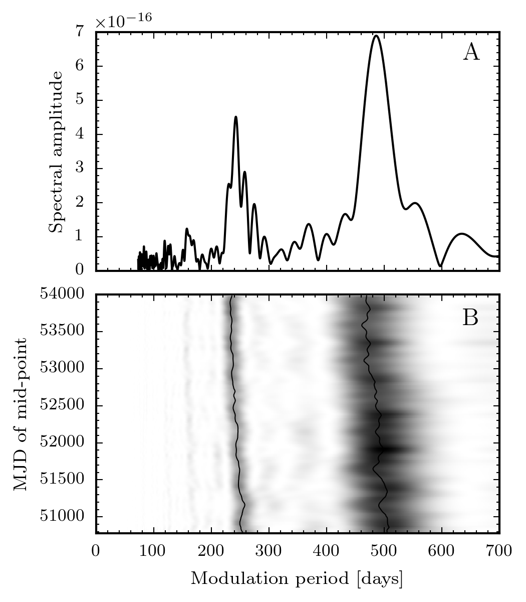
Figure 1: A: The Lomb-Scargle estimate of the period spectrum of the spin-down rate residual using the entire duration of data. B: The period spectrum of the spin-down rate residual over a sliding window of approximately 2058 days, as a function of the window mid-point (on the y-axis).

This figure shows that the modulation period $P_{\rm mod}$ appears to be decreasing over time. Taking the major mode from the first and last sliding window we find that over a time span of $3200$ days the modulation period decreased from $505$ to $470$ days, corresponding to a rate of change of $\dot{P}_{\textrm{mod}}\approx-0.01$ s/s. We note that this estimate is inherently imprecise due to the fact that the Lomb-Scargle method is fitting a constant period sinusoid to data which is best described by a sinusoid with changing period. Nevertheless, it does provide a rough estimate. To underline the significance of this observed $\dot{P}_{\textrm{mod}}$, we found the best-fit for a phenomological fixed-period sinusoidal model – two sinusoids at $P_{\textrm{mod}}$ and $P_{\textrm{mod}}/2$ with independent amplitudes and a relative phase – to the spin-down rate residual. We then generated $10^{4}$ realisations of central Gaussian noise with a standard deviation of $4.3\times 10^{-16}$ s^-2 (based on the standard-deviation of the residual after removing the best-fit sinusoidal model). Adding the best-fit signal to each noise realisation, we apply our Lomb-Scargle process to calculate the change in period (due purely to the noise fluctuations) and find that the maximum $|\dot{P}_{\textrm{mod}}|<10^{-7}$. This illustrates that the observed $\dot{P}_{\textrm{mod}}\sim-0.01$ for PSR B1828-11 is highly unlikely to be due to Gaussian noise fluctuations alone.

This shortening of the modulation period provides a new observational feature that needs to be accommodated by any model trying to describe this data. For example in the planetary hypothesis this would require that the two planets maintain orbital resonance while inspiralling. For the magnetospheric switching model proposed by Perera et al. (2015) and further studied in Paper I, it is unclear how this could be incorporated, given the purely phenomenological nature of this model. In the future it would interesting to understand this observation in the context of other models; in this work we explore how this feature is accommodated within the precession model of Paper I.

3 Data analysis methodology

In Paper I we performed a Bayesian model comparison between precession (with non-circular beam geometry) and magnetospheric switching for the observed long-term variations in spin-down rate and beam-width of PSR B1828-11. Because of the purely phenomenological nature of the switching model, no physical priors on its parameters were readily available and we therefore resorted to a two-step approach: first we performed parameter-estimation for both models on the spin-down data alone, by using wide flat priors for both models. Then we used the resulting posteriors as priors for a model comparison on the beam-width data. This yielded odds of $10^{2.7\pm 0.5}$ in favour of the precession model.

In this work, we focus on physical generalisations of the precession model and compare these to the ‘base’ precession model. The competing generalised precession models share the parameters of the base-model, but extend them with additional physical parameters that are allowed to be nonzero. The base-model priors can be thought of as effectively expressing certainty for these additional parameters to vanish exactly, while the generalised models relax this restriction and instead use plausible nonzero priors for them. This allows us to directly perform model comparison between base and generalised models on the full data set comprising both spin-down and beam-width data.

We define the data $\mathcal{D}$ as $N$ observed $\dot{\nu}^{i}$ values and $M$ observed $W_{10}^{j}$ values. We denote as $\sigma_{\dot{\nu}}$ and $\sigma_{W_{10}}$ the (assumed Gaussian) noise level for each type of observation. The likelihood for the data (see Section 2 of Paper I) given by model $\mathcal{M}$ with model parameters $\boldsymbol{\lambda}$ is then

$$P(\mathcal{D}|\mathcal{M},\vartheta)= {\prod_{i=1}^{N}}P(\dot{\nu}^{i}|\mathcal{M},\boldsymbol{\lambda},\sigma_{\dot{\nu}}){\prod_{j=1}^{M}}P(W_{10}^{j}|\mathcal{M},\boldsymbol{\lambda},\sigma_{W_{10}}),$$ (1)

where $\vartheta=[\boldsymbol{\lambda},\sigma_{\dot{\nu}},\sigma_{W_{10}}]$ is the full set of parameters. To approximate the posterior density of these parameters, we use the Foreman-Mackey et al. (2013) implementation of the affine-invariant parallel-tempered MCMC sampler (Goodman & Weare, 2010); the exact methodology is described in Appendix A of Paper I. We then use thermodynamic integration (Goggans & Chi, 2004) to estimate the marginal likelihood of a given model (see Section 4 of Paper I) and hence the odds-ratio between models setting the prior ratio to unity. We use the posterior odds between models to quantify how much, if at all, each extension improves the power of the model to describe the data, compared to the base-model. This depends on both the improvement to fit the data as well as on the respective prior volume of the extension parameters, which provides an effective ‘Occam factor’ against the extension.

4 The precession base-model

We begin by introducing our base-model, the precession model based on the treatment given in Paper I. It is against this which the extended models will be compared.

4.1 Defining the base-model

We consider a biaxial star, spinning down by electromagnetic torque from the magnetic dipole $\mathbf{m}$, which forms an angle $\chi$ with the symmetry axis of the star. Following Jones & Andersson (2001), we define $\theta$ as the wobble angle between the symmetry axis and the angular momentum vector. Precession produces modulations with period$P_{\mathrm{fp}}$ in the rotation of the magnetic axis. As a result, the spin-down rate and beam-width are modulated on the free precession period.

Combining precession with a generalisation of the vacuum dipole torque and allowing for an arbitrary braking index $n$, we show in Appendix A that the spin-down rate, in the small-$\theta$ limit, is given by

$$\begin{split}\dot{\nu}(t)=&\dot{\nu}_{0}+\ddot{\nu}_{0}(t-t_{\textrm{ref}})\\ &-\dot{\nu}_{0}\theta\left[2\cot\chi\sin(\psi(t))-\frac{\theta}{2}\cos(2\psi(t))\right],\end{split}$$ (2)

where $[\dot{\nu}_{0},\ddot{\nu}_{0}]$ are the fixed frequency derivatives defined at a reference time $t_{\textrm{ref}}$ and $\psi$ is one the three Euler angles describing the orientation of the star (see for example Landau & Lifshitz (1969)). We note that Equation (missing) 2 is equivalent to the results of Jones & Andersson (2001) and Link & Epstein (2001), although these previous works fixed the braking index to $n{=}3$. If the spin-down age is much longer than the precession period $P_{\mathrm{fp}}$, we have that

$$\psi(t)=-2\uppi\,\frac{t-t_{\textrm{ref}}}{P_{\mathrm{fp}}}+\psi_{0},$$ (3)

in which we have implicitly defined the precession period as

$$P_{\mathrm{fp}}=\frac{1}{\epsilon_{\mathrm{p}}\,\nu(t)\,\cos\theta},$$ (4)

where $\nu(t)$ is the instantaneous spin-frequency at time $t$, and

$$\epsilon_{\mathrm{p}}=\frac{\Delta I_{\rm d}}{I_{\rm prec}},$$ (5)

where $\Delta I_{\rm d}$ is the stellar deformation caused by elastic/magnetic strains, while $I_{\rm prec}$ is that part of the star that participates in the free precession. We can expect $I_{\rm crust}<I_{\rm prec}<I_{*}$; see Jones & Andersson (2001) for details.

Formally, the spin frequency $\nu(t)$ is the integral of Equation (missing) 2. However, the sinusoidal variations due to precession will average to zero over an integer number of cycles. Therefore, we will neglect the residual modulations, which will have a negligible effect on the precession period, and approximate the spin frequency in Equation (missing) 4 by

$$\nu(t)=\nu_{0}+\dot{\nu}_{0}\,(t-t_{\textrm{ref}})+\frac{\ddot{\nu}_{0}}{2}\,(t-t_{\textrm{ref}})^{2},$$ (6)

where $\nu_{0}$ is the fixed frequency of the star at $t_{\textrm{ref}}$. We will define $t_{\textrm{ref}}$ at the epoch given in the ATNF (Manchester et al., 2005) entry for PSR B1828-11. This reference time, the frequency and its derivatives, and other useful quantities are listed in Table 1.

Table 1: Table of astrophysical data for B1828-11 taken from the ATNF pulsar catalogue (Manchester et al., 2005), available at %****␣Paper_B1828-11_DataAnalysis_II.tex␣Line␣450␣****www.atnf.csiro.au/people/pulsar/psrcat.

Parameter	ATNF value
$t_{\textrm{ref}}$	MJD 49621
$\nu_{0}$	$2.46887171470\pm 7\times 10^{-11}$   Hz
$\dot{\nu}_{0}$	$-3.658728\times 10^{-13}\pm 5\times 10^{-19}$   Hz/s
$\ddot{\nu}_{0}$	$8.72\times 10^{-25}\pm 9\times 10^{-27}$   Hz/s2
$\tau_{\mathrm{age}}=-\nu_{0}/\dot{\nu}_{0}$	$1.07\times 10^{5}$ yrs
$n=\ddot{\nu}_{0}\nu_{0}/\dot{\nu}_{0}^{2}$	$16.08\pm 0.7$
Distance	3.58 kpc

The pulse beam-width $W_{10}$ is defined as the width of the pulse at 10% of the observed peak intensity. This beam-width depends on the motion of the dipole $\mathbf{m}$, how the intensity of emission varies across the beam, and on the relative position of the observer and the beam. The angle $\Theta$ between the dipole $\mathbf{m}$ and the angular momentum $\mathbf{J}$ can be expressed as

$$\Theta(t)=\cos^{-1}\left(\sin\theta\sin\chi\sin(\psi(t))+\cos\theta\cos\chi\right),$$ (7)

which describes the polar motion of $\mathbf{m}$ in the inertial frame (Bisnovatyi-Kogan et al., 1990; Jones & Andersson, 2001). Let $\iota$ denote the angle between the observing direction and $\mathbf{J}$, and so the latitudinal separation between observer and beam is given simply by $\Delta\Theta(t)=\Theta(t)-\iota$.

In Paper I we first considered an emission model where the intensity of the emitted radiation is circularly symmetric around the dipole $\mathbf{m}$ with a radial Gaussian fall-off. However, this simple model is unable to account for the observed variations in $W_{10}$, and we therefore extended the model to allow for the longitudinal width of the Gaussian describing the intensity to depend on the latitude $\Delta\Theta(t)$ of the cut made through the beam; this was found to produce good agreement with observations (similar conclusions have previously been obtained by Link & Epstein (2001)). This results in a beam-width expression of the form

$$W_{10}(t)=\frac{1}{\nu(t)\,\uppi}\sqrt{\frac{2\ln 10}{\sin\Theta(t)\,\sin\iota}}\left(\rho_{2}^{0}+\rho_{2}^{\prime\prime}\,\Delta\Theta(t)^{2}\right),$$ (8)

where $\rho_{2}^{0}$ is the width of the Gaussian intensity at $\Delta\Theta=0$ and $\rho_{2}^{\prime\prime}$ describes the variation in intensity with $\Delta\Theta$; see Paper I. Our formulation of the base-model is now complete: Equation (missing) 2 is the base spin-down model and Equation (missing) 8 is the base beam-width model.

This formulation of the base precession model differs from that used in Paper I in two ways. First, in Paper I, $P_{\mathrm{fp}}$ was a constant model parameter. But in Equation (missing) 4, we now express the precession period $P_{\mathrm{fp}}$ in terms of the fundamental model parameters: the instantaneous spin-frequency $\nu(t)$, wobble angle $\theta$, and the deformation $\epsilon_{\mathrm{p}}$. While this change of parameterisation provides a more complete description (in that it includes the time evolution of $P_{\mathrm{fp}}$ with $\nu(t)$), it was found to produce no significant change in the fit. Second, the sign of the first term of Equation (missing) 3 was positive in Eqn. (16) of Paper I, but is now negative; this change amounts to a redefinition of $P_{\mathrm{fp}}$ which was done such that for an oblate star, $\epsilon_{\mathrm{p}}$ and $P_{\mathrm{fp}}$ are both positive, while for a prolate star both these quantities are formally negative. As the spin-down rate and beam-width of the precession model (Equation (missing) 2 and Equation (missing) 8 respectively) are invariant to this change of sign (modulo addition of $\uppi$ to $\psi_{0}$), the redefinition of $P_{\mathrm{fp}}$ makes no substantial difference to the model.

The base-model and all extensions considered in this work are subject to two symmetries which are important when interpreting our results. First, as a consequence of the invariant nature of the spin-down rate and beam-width to the sign of $\epsilon_{\mathrm{p}}$, the data cannot fix the overall sign of $\epsilon_{\mathrm{p}}$. We restrict this symmetry by choosing $\epsilon_{\mathrm{p}}>0$ in the prior, but we note that solutions where $\epsilon_{\mathrm{p}}\rightarrow-\epsilon_{\mathrm{p}}$ are equally valid. Second, it was noted by Arzamasskiy et al. (2015) that the spin-down rate in the precession model is symmetric under the substitution $\theta\leftrightarrow\chi$ (we discuss how this can be derived for Equation (missing) 2 in Appendix A); in our model, this is also true for the beam-width. For both the spin-down and beam-width models, this is fundamentally due to the symmetry of $\chi$ and $\theta$ in Equation (missing) 7. In our analysis, we consider only the ‘large $\chi$’ model (as defined by Arzamasskiy et al. (2015)) and restrict this symmetry in the derivation by assuming that $\theta\ll 1$ and in the choice of prior. But, rederiving the equations with $\chi\ll 1$ instead results in Equation (missing) 2 with $\theta\leftrightarrow\chi$. Therefore, all models and parameter estimation considered in this work can equally be applied to the ‘small $\chi$’ model by interchanging $\chi$ and $\theta$. These symmetries may be important to consider when relating the model extension to physical theories.

4.2 Applying the base-model to the data

The base-model consists of the spin-down and beam-width predictions given in Equation (missing) 2 and Equation (missing) 8. Before applying these to the data, we first define our priors. Since we will use the same priors for these parameters when considering the extended models in the following sections, their prior volume won’t have an impact on the model-comparison odds.

The full set of priors are listed in Table 2 and we now describe our choices in detail. For the spin frequency and frequency derivatives we apply astrophysical priors based on data from the ATNF database (which is listed in Table 1). Specifically, we use normal distributions with mean and standard-deviation given by the ATNF values. For the deformation $\epsilon_{\mathrm{p}}$ we use the absolute value of a normal distribution as prior, ensuring our gauge choice of $\epsilon_{\mathrm{p}}\geq 0$. The normal distribution has zero mean, and a standard deviation of $10^{-8}$, the approximate known value of $\epsilon_{\mathrm{p}}$ (Paper I). For the angles $\theta$ and $\chi$ we restrict their domain to solutions where the wobble angle $\theta$ is small while the magnetic inclination $\chi$ is close to orthogonal (the ‘large $\chi$’ model, for more details see Appendix A)). The beam-width parameters ($\rho_{2}^{0}$ and $\rho_{2}^{\prime\prime}$) use priors from Paper I, which were chosen to give a range of beam-widths up to $10\%$ of the period and allow for some non-circularity. Finally the phase is given a uniform prior over its domain and we use uniform priors for $\sigma_{\dot{\nu}}$ and $\sigma_{W_{10}}$ from a crude estimate of the data.

Table 2: Prior distributions and a posterior distribution summary for the base-model parameters.

	Prior	Posterior median $\pm$ s.d.	Units
$\nu_{0}$	$\mathcal{N}$(2.46887171470, ${7.0}{\times}10^{\textrm{-}11}$)	2.47$\pm$${7.0}{\times}10^{\textrm{-}11}$	Hz
$\dot{\nu}_{0}$	$\mathcal{N}$(${\text{{-}}3.658728}{\times}10^{\textrm{-}13}$, ${5.0}{\times}10^{\textrm{-}19}$)	${\text{{-}}3.66}{\times}10^{\textrm{-}13}$$\pm$${5.0}{\times}10^{\textrm{-}19}$	Hz/s
$\ddot{\nu}_{0}$	$\mathcal{N}$(${8.72}{\times}10^{\textrm{-}25}$, ${9.0}{\times}10^{\textrm{-}27}$)	${8.73}{\times}10^{\textrm{-}25}$$\pm$${9.0}{\times}10^{\textrm{-}27}$	Hz/s2
$\epsilon_{\mathrm{p}}$	$|\mathcal{N}$(0, ${1}{\times}10^{\textrm{-}8}$)$|$	${9.67}{\times}10^{\textrm{-}9}$$\pm$${1.1}{\times}10^{\textrm{-}11}$
$\theta$	Unif(0, 0.1)	0.0490$\pm$0.0020	rad
$\chi$	Unif($2\uppi/5$, $\uppi/2$)	1.5519$\pm$0.0013	rad
$\psi_{0}$	Unif(0, $2\uppi$)	5.4821$\pm$0.0456	rad
$\rho_{2}^{0}$	Unif(0, 0.1464)	0.0246$\pm$0.0004	rad
$\rho_{2}^{\prime\prime}$	$\mathcal{N}$(0, 6.83)	3.36$\pm$0.4	rad${}^{\textrm{-}2}$
$\cos(\iota)$	Unif(-1, 1)	${7.57}{\times}10^{\textrm{-}3}$$\pm$${2.1}{\times}10^{\textrm{-}3}$
$\sigma_{\dot{\nu}}$	Unif(0, ${1}{\times}10^{\textrm{-}15}$)	${4.09}{\times}10^{\textrm{-}16}$$\pm$${1.9}{\times}10^{\textrm{-}17}$	$\mathrm{s}^{\textrm{-}2}$
$\sigma_{W_{10}}$	Unif(0, ${5.0}{\times}10^{\textrm{-}3}$)	${1.59}{\times}10^{\textrm{-}3}$$\pm$${4.3}{\times}10^{\textrm{-}5}$	s

We run MCMC simulations applying the base-model to the data under these priors and check that they converge and properly sample the posterior. In Figure 2 we show the spin-down and beam-width data together with the maximum posterior estimate (MPE) solution of the model, i.e. using the parameters with the highest posterior probability.

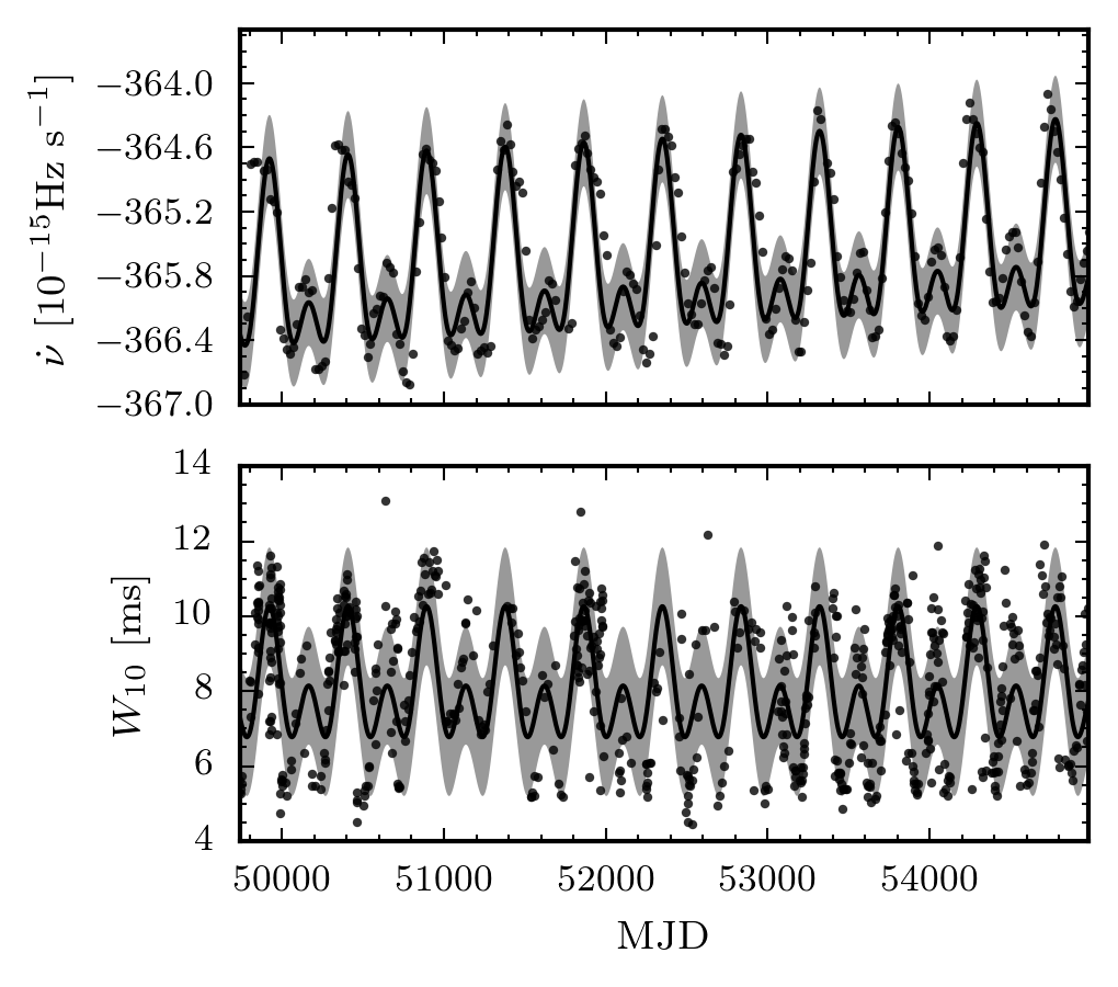
Figure 2: Comparison between the base-model (solid line) using maximum-posterior parameter estimates (MPE) and the observed spin-down and beam-width data (black dots). The shaded region indicates $1\,\sigma$ of the estimated noise level in the spin-down and beam-width data, respectively.

The samples from the converged MCMC chains are used to estimate the posterior distributions, which we find to be Gaussian-like, and which we summarise in the second column of Table 2 by their median and standard deviation.

Compared to Paper I this base-model already contains one model extension: allowing for variation in $P_{\mathrm{fp}}$ due to $\nu(t)$, as seen in Equation (missing) 4. However, this does not make any appreciable difference to the result in that there is no noticeable difference between the two panels of Figure 2 and Figure 7B and Figure 11B of Paper I. Furthermore, this extension does not explain the observed changing modulation period discussed in section 2. In order to see this quantitatively, we expand Equation (missing) 4 to first order as

$$P_{\mathrm{fp}}\approx\frac{1}{\epsilon_{\mathrm{p}}\nu_{0}\cos\theta}\left(1-(t-t_{\textrm{ref}})\frac{\dot{\nu}_{0}}{\nu_{0}}\right).$$ (9)

Since $\dot{\nu}_{0}<0$ this produces an increasing precession period, which over the observation span produces a fractional change in precession period of $\sim 7{\times}10^{-5}$. Hence, the effect of the spin-down is too small and of the wrong sign to explain the observations of section 2.

From Equation (missing) 4 we see that there are two further possible ways that $P_{\mathrm{fp}}$ can evolve: either the wobble angle $\theta$ or the deformation $\epsilon_{\mathrm{p}}$ must evolve (or both). In the following sections, we will consider these possibilities in turn and evaluate the improvements in the power of the respective model to describe the data by computing their odds compared to the base-model.

5 Secular evolution of the wobble angle: the $\dot{\theta}$-model

There are two reasons for allowing a secular evolution of the precession wobble angle. Firstly, from Equation (missing) 4 we see that such an evolution could potentially drive a change in the precession period explaining the results of section 2. However, simple estimates show that the required rate of variation in $\theta$ is much too large to be consistent with the observations; we give such arguments in subsection 5.1 below. Secondly, and perhaps more fundamentally, in the precessional interpretation, dissipative processes are expected to exist and should damp the wobble angle, which would provide insights into the crust-core coupling (see for example Sedrakian et al. (1999) and Levin & D’Angelo (2004)).

We model this in the simplest way by assuming that $\theta$ changes linearly in time as

$$\theta(t)=\theta+\dot{\theta}\,(t-t_{\textrm{ref}}).$$ (10)

The base-model spin-down rate of Equation (missing) 2 was derived under the assumption that $\theta$ is constant. However, when rederiving this expression with an evolving $\theta$ according to Equation (missing) 10, we find that (to first order) the expression remains valid with the simple substitution $\theta\rightarrow\theta(t)$.

5.1 Can a changing $\theta$ explain the observed decrease in precession period?

Using the following simple argument, we can see that a nonzero $\dot{\theta}$ cannot consistently explain the observed decrease in precession period of $\dot{P}_{\mathrm{fp}}\approx-0.01$ s/s found in section 2. Taking the time-derivative of Equation (missing) 4 with $\theta=\theta(t)$ (and dropping a negligible contribution $P_{\mathrm{fp}}/\tau_{\mathrm{age}}\sim 10^{-5}$ s/s to $\dot{P}_{\mathrm{fp}}$) we can estimate the required $\dot{\theta}$ as

$$\dot{\theta}=\frac{\dot{P}_{\mathrm{fp}}}{P_{\mathrm{fp}}}\,\cot\theta\approx-5\times 10^{-9}\textrm{rad/s}\,,$$ (11)

therefore

$$\tau_{\theta}\equiv\frac{\theta}{|\dot{\theta}|}=\frac{\theta}{\cot\theta}\,\frac{P_{\mathrm{fp}}}{|\dot{P}_{\mathrm{fp}}|}\approx\frac{1}{400}\,\frac{P_{\mathrm{fp}}}{\dot{P}_{\mathrm{fp}}}\sim 0.34\,\mathrm{years}\,.$$ (12)

where we used the base-model posterior estimates from Table 2 for $\theta$ and for $P_{\mathrm{fp}}$ (these values are derived assuming that $\dot{\theta}=0$, however, as shown later in Table 3 they are consistent with those found when this assumption is relaxed). Similarly, with the estimate of Equation (missing) 11 the predicted relative change in the spin-down modulation amplitude from Equation (missing) 2 over the observation period of $T\approx 5000$ days would amount to

$$\frac{\dot{\theta}T}{\theta}\approx-46.8\,.$$ (13)

This level of change in $\theta$ is inconsistent with the observed spin-down variations, which are well described by a model with an approximately constant $\theta$ (e.g. see Figure 2).

We can therefore conclude that changes in $\theta$ are unable to explain the decrease in modulation period. Fundamentally, this stems from the fact that the dependence of the modulation amplitude on $\theta$ is $\propto\theta$, while the dependence of $P_{\mathrm{fp}}$ is $\propto 1+\theta^{2}/2$ for $\theta\ll 1$.

5.2 Applying the $\dot{\theta}$-model to the data

We choose a weakly-informative prior for the additional model parameter $\dot{\theta}$: a central normal distribution with standard-deviation of $2.2\times 10^{-10}$ rad/s, which is the value one would get if $\dot{\theta}\sim 2\theta/T$, so effectively this allows $\theta$ to change by twice its magnitude over the observation time $T$. Using such a wide prior allows us to be confident that the posterior upper limit on $\dot{\theta}$ will be informed by the data and not the result of an overly-constrained prior.

The resulting posteriors for $\theta$ and $\dot{\theta}$ are shown in Figure 3 and the posteriors for all model parameters are summarised in Table 3 alongside the priors (which are identical to those of the base-model).

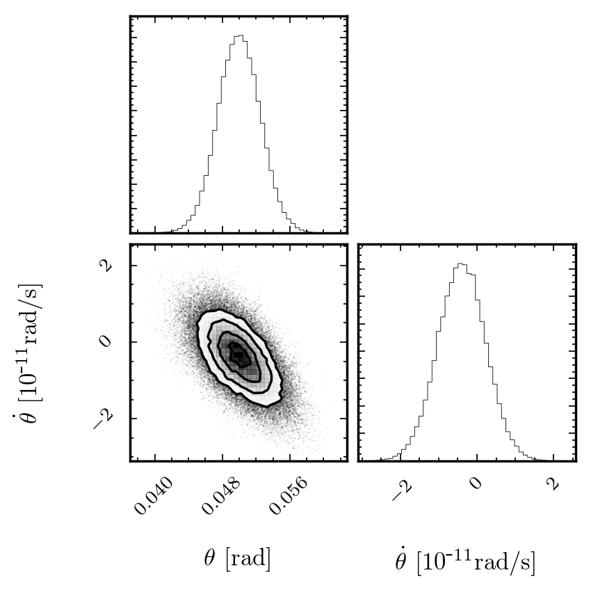
Figure 3: Posterior probability distributions for the wobble angle $\theta$ and its rate of change $\dot{\theta}$ in the $\dot{\theta}$-model.

Table 3: Prior distributions and a posterior distribution summary for the $\dot{\theta}$-model parameters.

	Prior	Posterior median $\pm$ s.d.	Units
$\nu_{0}$	$\mathcal{N}$(2.46887171470, ${7.0}{\times}10^{\textrm{-}11}$)	2.47$\pm$${7.0}{\times}10^{\textrm{-}11}$	Hz
$\dot{\nu}_{0}$	$\mathcal{N}$(${\text{{-}}3.658728}{\times}10^{\textrm{-}13}$, ${5.0}{\times}10^{\textrm{-}19}$)	${\text{{-}}3.66}{\times}10^{\textrm{-}13}$$\pm$${5.0}{\times}10^{\textrm{-}19}$	Hz/s
$\ddot{\nu}_{0}$	$\mathcal{N}$(${8.72}{\times}10^{\textrm{-}25}$, ${9.0}{\times}10^{\textrm{-}27}$)	${8.73}{\times}10^{\textrm{-}25}$$\pm$${8.9}{\times}10^{\textrm{-}27}$	Hz/s2
$\epsilon_{\mathrm{p}}$	$|\mathcal{N}$(0, ${1}{\times}10^{\textrm{-}8}$)$|$	${9.67}{\times}10^{\textrm{-}9}$$\pm$${1.2}{\times}10^{\textrm{-}11}$
$\theta$	Unif(0, 0.1)	0.0500$\pm$0.0025	rad
$\dot{\theta}$	$\mathcal{N}$(0, ${2.2}{\times}10^{\textrm{-}10}$)	${\text{{-}}3.97}{\times}10^{\textrm{-}12}$$\pm$${6.3}{\times}10^{\textrm{-}12}$	rad/s
$\chi$	Unif($2\uppi/5$, $\uppi/2$)	1.5519$\pm$0.0013	rad
$\psi_{0}$	Unif(0, $2\uppi$)	5.4688$\pm$0.0494	rad
$\rho_{2}^{0}$	Unif(0, 0.1464)	0.0246$\pm$0.0004	rad
$\rho_{2}^{\prime\prime}$	$\mathcal{N}$(0, 6.83)	3.33$\pm$0.4	rad${}^{\textrm{-}2}$
$\cos(\iota)$	Unif(-1, 1)	${7.51}{\times}10^{\textrm{-}3}$$\pm$${2.1}{\times}10^{\textrm{-}3}$
$\sigma_{\dot{\nu}}$	Unif(0, ${1}{\times}10^{\textrm{-}15}$)	${4.09}{\times}10^{\textrm{-}16}$$\pm$${1.9}{\times}10^{\textrm{-}17}$	$\mathrm{s}^{\textrm{-}2}$
$\sigma_{W_{10}}$	Unif(0, ${5.0}{\times}10^{\textrm{-}3}$)	${1.59}{\times}10^{\textrm{-}3}$$\pm$${4.2}{\times}10^{\textrm{-}5}$	s

The $\theta$ posterior is found to be essentially unchanged with respect to the base-model. The $\dot{\theta}$ posterior shows a substantial amount of ‘shrinkage’ compared to its prior range, but is fully consistent with $\dot{\theta}=0$ and therefore provides no evidence that $\theta$ is actually changing. Nevertheless, we can use this to place constraints on the timescale of $\theta$-changes by defining $\tau_{\theta}\equiv|\theta/\dot{\theta}|$ and using the samples from Figure 3 to estimate the posterior distribution for $\tau_{\theta}$, which is shown in Figure 4. This figure shows that there is little support for variation timescales below $\sim 100\,\mathrm{years}$ (confirming that the required timescale for $\tau_{\theta}$ to explain the changing modulation period given in Equation (missing) 12 is too short). The distribution has a long tail, allowing for much longer timescales. The median of the distribution is $307.7\,\mathrm{years}$ and we can place a $95\%$ credible lower limit of $\tau_{\theta}>114.3\,\mathrm{years}$.

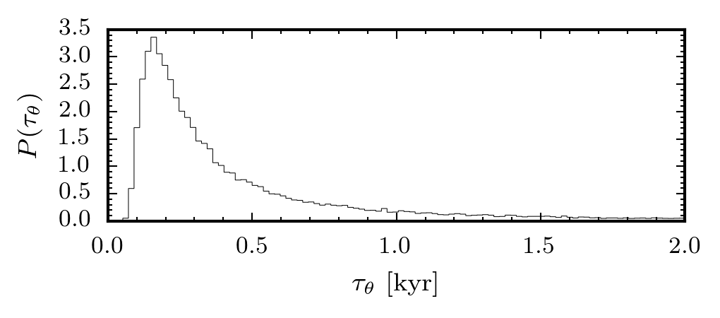
Figure 4: The posterior distribution for $\tau_{\theta}\equiv|\theta/\dot{\theta}|$ under the $\dot{\theta}$-model.

The odds between the $\dot{\theta}$-model compared to the base-model are found as $10^{-1.70\pm 1.39}$, i.e. weak evidence against this extension. This shows the effect of the built-in Bayesian ‘Occam factor’: the extension of allowing $\dot{\theta}\not=0$ (which can only improve the fit to the data) does not provide a sufficient improvement in likelihood compared to the increase in prior volume.

6 Secular evolution of the deformation: the $\dot{\epsilon}_{\mathrm{p}}$-model

After ruling out variations in $\nu$ and $\theta$ in the previous sections as the cause for the observed level of $\dot{P}_{\mathrm{fp}}$, we see from Equation (missing) 4 that this leaves only variations in the deformation $\epsilon_{\mathrm{p}}$ as a possible explanation. In this section and section 8, we consider two distinct types of time-evolution in $\epsilon_{\mathrm{p}}$: firstly the $\dot{\epsilon}_{\mathrm{p}}$-model, a slow continuous change (approximated by the linear term) in $\epsilon_{\mathrm{p}}$, and then the $\Delta\epsilon_{\mathrm{p}}$-model, a series of distinct ‘jumps’ in $\epsilon_{\mathrm{p}}$. These are just two possible phenomological models which are not founded in any physical theory, instead they are chosen simply to model two distinctive behaviours.

6.1 Defining the $\dot{\epsilon}_{\mathrm{p}}$-model

We consider the simplest continuously changing deformation model by including a linear term (which also describes a larger class of sufficiently-slow continuous change in $\epsilon_{\mathrm{p}}$):

$$\epsilon_{\mathrm{p}}(t)=\epsilon_{\mathrm{p}}+\dot{\epsilon}_{\mathrm{p}}\,(t-t_{\textrm{ref}}).$$ (14)

We will discuss some potential physical mechanisms for such a secular change in section 10.

Allowing for a time-varying $\epsilon_{\mathrm{p}}(t)$ in Equation (missing) 4 and assuming this accounts for the majority of the change in $P_{\mathrm{fp}}$, we obtain

$$\frac{\dot{P}_{\mathrm{fp}}}{P_{\mathrm{fp}}}\approx-\frac{\dot{\epsilon}_{\mathrm{p}}}{\epsilon_{\mathrm{p}}}\equiv-\frac{1}{\tau_{\epsilon}}\,,$$ (15)

where we have defined the characteristic timescale $\tau_{\epsilon}$ for the rate of change in $\epsilon_{\mathrm{p}}$.

Given that $P_{\mathrm{fp}}$ is decreasing with time (c.f. section 2), for $\epsilon_{\mathrm{p}}>0$ this implies $\dot{\epsilon}_{\mathrm{p}}>0$, while for $\epsilon_{\mathrm{p}}<0$ this would correspond to $\dot{\epsilon}_{\mathrm{p}}<0$. As previously mentioned, we are unable to determine the sign of $\epsilon_{\mathrm{p}}$ from our current precession model, but in either case the magnitude of the deformation has to be increasing, i.e. $d|\epsilon_{\mathrm{p}}|/dt>0$, in order to account for the observed decrease in $P_{\mathrm{fp}}$.

From Equation (missing) 15 we can estimate the required $\dot{\epsilon}_{\mathrm{p}}$ for the observed $\dot{P}_{\mathrm{fp}}\approx-0.01$ s/s as found in section 2, which yields $\dot{\epsilon}_{\mathrm{p}}\approx 2\times 10^{-18}$ s^-1. We use this as the scale for a central Gaussian prior on $\dot{\epsilon}_{\mathrm{p}}$ as

$$\dot{\epsilon}_{\mathrm{p}}\sim|N\left(0,\,2{\times}10^{-18}\right)|,$$ (16)

where we restrict ourselves to positive values in accordance to our gauge choice of $\epsilon_{\mathrm{p}}>0$.

This prior is weakly informed by the data, but we could equally well consider a less-informed choice of, say, allowing $\epsilon_{\mathrm{p}}$ to double in size over the observation timescale $T=5000\,$days, which would yield a prior scale of $\dot{\epsilon}_{\mathrm{p}}\sim 2{\times}10^{-17}\mathrm{s}^{-1}$. This is only a factor of 10 wider compared to Equation (missing) 16, and would be expected to reduce the odds by about one order of magnitude at most via the larger ‘Occam factor’ (i.e. prior volume). Re-running the analysis with the wider prior confirms this, as we obtain odds that are reduced by a factor of $\sim 5$ compared to using Equation (missing) 16, while yielding essentially unchanged posteriors.

6.2 Applying the $\dot{\epsilon}_{\mathrm{p}}$-model to the data

The estimated posteriors distribution for selected model parameters are plotted in Figure 5 and the entire set is summarised in Table 4 along with their prior distributions. Comparing this to the base-model, two features are notable: the posterior mean of $\epsilon_{\mathrm{p}}$ is fractionally smaller, and $\dot{\epsilon}_{\mathrm{p}}$ has a posterior mean quite different from its prior, with a positive mean and essentially zero probability of $\dot{\epsilon}_{\mathrm{p}}=0$. Since $\dot{\epsilon}_{\mathrm{p}}>0$, the deformation is growing with time as expected from the observation that $P_{\mathrm{fp}}$ is decreasing.

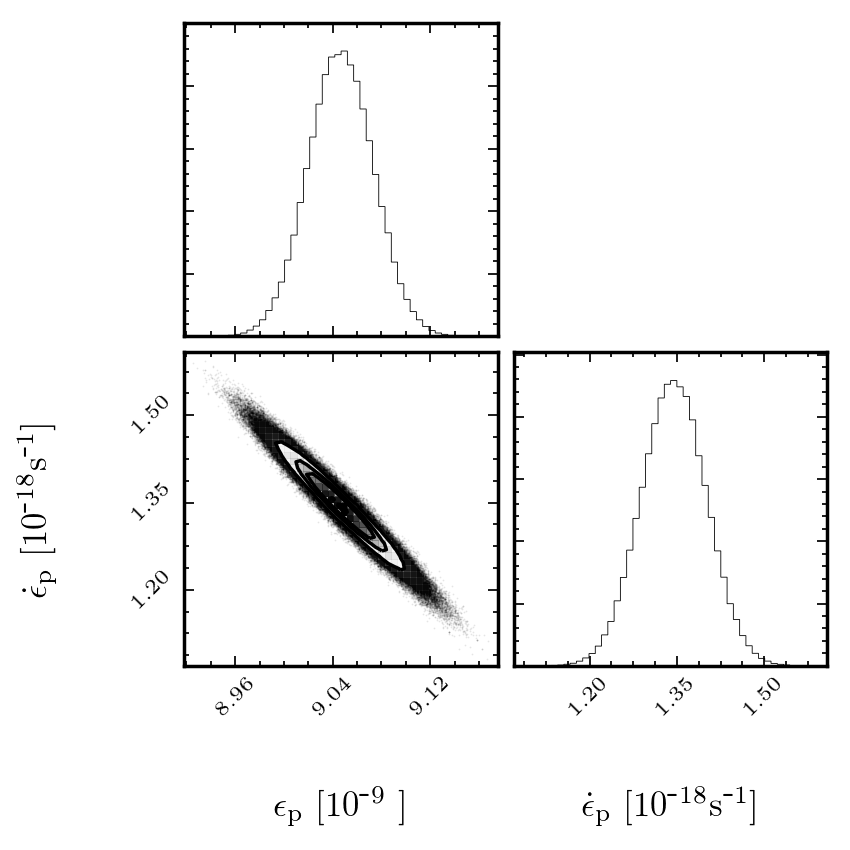
Figure 5: Posterior probability distributions for the deformation $\epsilon_{\mathrm{p}}$ and its rate of change $\dot{\epsilon}_{\mathrm{p}}$ in the $\dot{\epsilon}_{\mathrm{p}}$-model.

Table 4: Prior distributions and a posterior distribution summary for the $\dot{\epsilon}_{\mathrm{p}}$-model parameters.

	Prior	Posterior median $\pm$ s.d.	Units
$\nu_{0}$	$\mathcal{N}$(2.46887171470, ${7.0}{\times}10^{\textrm{-}11}$)	2.47$\pm$${7.0}{\times}10^{\textrm{-}11}$	Hz
$\dot{\nu}_{0}$	$\mathcal{N}$(${\text{{-}}3.658728}{\times}10^{\textrm{-}13}$, ${5.0}{\times}10^{\textrm{-}19}$)	${\text{{-}}3.66}{\times}10^{\textrm{-}13}$$\pm$${5.0}{\times}10^{\textrm{-}19}$	Hz/s
$\ddot{\nu}_{0}$	$\mathcal{N}$(${8.72}{\times}10^{\textrm{-}25}$, ${9.0}{\times}10^{\textrm{-}27}$)	${8.75}{\times}10^{\textrm{-}25}$$\pm$${8.9}{\times}10^{\textrm{-}27}$	Hz/s2
$\epsilon_{\mathrm{p}}$	$|\mathcal{N}$(0, ${1}{\times}10^{\textrm{-}8}$)$|$	${9.05}{\times}10^{\textrm{-}9}$$\pm$${2.7}{\times}10^{\textrm{-}11}$
$\dot{\epsilon}_{\mathrm{p}}$	$|\mathcal{N}$(0, ${2}{\times}10^{\textrm{-}18}$)$|$	${1.34}{\times}10^{\textrm{-}18}$$\pm$${5.6}{\times}10^{\textrm{-}20}$	s${}^{\textrm{-}1}$
$\theta$	Unif(0, 0.1)	0.0560$\pm$0.0011	rad
$\chi$	Unif($2\uppi/5$, $\uppi/2$)	1.5529$\pm$0.0007	rad
$\psi_{0}$	Unif(0, $2\uppi$)	4.7725$\pm$0.0404	rad
$\rho_{2}^{0}$	Unif(0, 0.1464)	0.0236$\pm$0.0003	rad
$\rho_{2}^{\prime\prime}$	$\mathcal{N}$(0, 6.83)	3.26$\pm$0.2	rad${}^{\textrm{-}2}$
$\cos(\iota)$	Unif(-1, 1)	${6.69}{\times}10^{\textrm{-}3}$$\pm$${1.3}{\times}10^{\textrm{-}3}$
$\sigma_{\dot{\nu}}$	Unif(0, ${1}{\times}10^{\textrm{-}15}$)	${2.57}{\times}10^{\textrm{-}16}$$\pm$${1.2}{\times}10^{\textrm{-}17}$	$\mathrm{s}^{\textrm{-}2}$
$\sigma_{W_{10}}$	Unif(0, ${5.0}{\times}10^{\textrm{-}3}$)	${1.47}{\times}10^{\textrm{-}3}$$\pm$${4.0}{\times}10^{\textrm{-}5}$	s

As pointed out earlier, we recall that due to the degeneracy of the spin-down rate and beam-width with respect to the sign of $\epsilon_{\mathrm{p}}$, this should therefore generally be interpreted as $|\dot{\epsilon}_{\mathrm{p}}|>0$.

In Figure 6 we plot the MPE spin-down and beam-width functions given by the model together with the observed data. Comparing this to Figure 2 it is evident that the model extension of Equation (missing) 14, allowing for evolution of the precession period via $\dot{\epsilon}_{\mathrm{p}}$, noticeably improves the description of the data compared to the base-model.

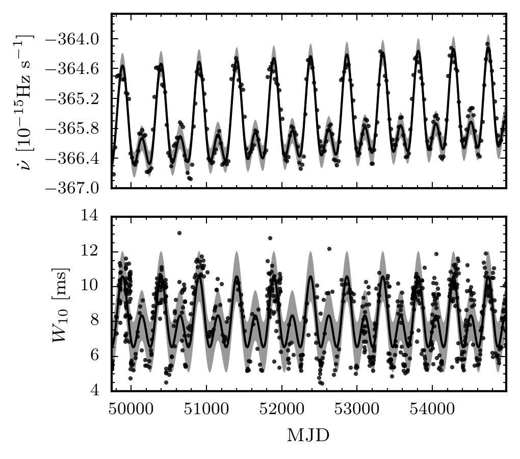
Figure 6: Comparison between the MPE $\dot{\epsilon}_{\mathrm{p}}$-model (solid line) and the observed spin-down and beam-width data (black dots). The shaded region indicates the estimated $1\,\sigma$ noise level.

This improvement is confirmed by the odds between the $\dot{\epsilon}_{\mathrm{p}}$-model and the base-model which are found as $10^{73.65\pm 0.97}$, i.e. decisive evidence in favour of an increasing deformation $|\epsilon_{\mathrm{p}}|$ as opposed to a constant.

To understand how the two data sources contribute to the total odds, we repeat the analysis on the two data sets independently and find that the odds for the spin-down data are $10^{49.35\pm 1.44}$ while the odds for the beam-width data are $10^{23.46\pm 1.83}$ such that the individual odds approximately sum to the combined odds. One would expect the odds to sum up this way if the posteriors (when conditioned on each data set individually) are consistent; we show this is the case in Appendix B. The independent odds show that each data set separately strongly favours the $\dot{\epsilon}_{\mathrm{p}}$-model, with the (clearly much cleaner) spin-down data providing stronger evidence than the beam-width data.

The large numerical values of the odds we obtain are related to the fact that for a Gaussian-noise model the log-odds scale linearly with the number of data points. For the spin-down data set, which consisted of $257$ data points, the average log-odds contributed by each point is $49.61/257\approx 0.19$, or a factor of $10^{0.19}\approx 1.6$ per data point to the odds itself. For the beam-width data, the corresponding numbers are $23.42/756\approx 0.03$, or a factor of $10^{0.03}\approx 1.07$ increase in odds per data point. This illustrates that it is the combination of many data points, each of which (on average) only modestly favours the $\dot{\epsilon}_{\mathrm{p}}$-model, that leads to the large overall odds.

The timescale of the inferred increase in deformation is seen to be quite short: from the MCMC samples we calculate the median and standard deviation of the corresponding timescale to be

$$\tau_{\epsilon}\equiv\frac{\epsilon_{\mathrm{p}}}{\dot{\epsilon}_{\mathrm{p}}}=213\pm 10\,\mathrm{years}.$$ (17)

7 Secular evolution of wobble angle and deformation: the $\{\dot{\theta},\dot{\epsilon}_{\mathrm{p}}\}$-model

In section 5 we showed that variations of $\theta$ cannot be responsible for the observed changing modulation period $P_{\mathrm{fp}}$. In the precession model considered here, the only plausible explanation for the decreasing $P_{\mathrm{fp}}$ comes from allowing for an increasing deformation $|\epsilon_{\mathrm{p}}|$. However, physically it is still quite plausible for the wobble angle $\theta$ to change over time, and at the minimum this allows us to set limits on the rate of change of $\theta$, which has potentially interesting implications for the crust-core coupling. In this section, we will therefore consider a combined extension allowing for both $\theta$ and $\epsilon_{\mathrm{p}}$ to undergo linear secular evolution. This will allow us to set more stringent and realistic limits on the allowed $\dot{\theta}$ rates than those provided in section 5.

7.1 Applying the $\{\dot{\theta},\dot{\epsilon}_{\mathrm{p}}\}$-model to the data

In order to extend the base-model with both Equation (missing) 10 and Equation (missing) 14, we simply use the same formulations and priors as those given in section 5 and section 6.

Figure 7 shows the posteriors obtained for the deformation $\epsilon_{\mathrm{p}}$, the wobble angle $\theta$, and their time-derivatives, and Table 5 summarises the posteriors found for all the model parameters. We note that the posterior for $\dot{\theta}$ has again a slightly negative mean, but a narrower width than in the $\dot{\theta}$-model shown in Figure 3. While the evolution in $\theta$ and $\epsilon_{\mathrm{p}}$ cannot be strictly separated, the evolution of the deformation $\epsilon_{\mathrm{p}}$ accounts mostly for the time varying modulation period, while the evolution of the wobble angle $\theta$ primarily probes the variation in amplitude.

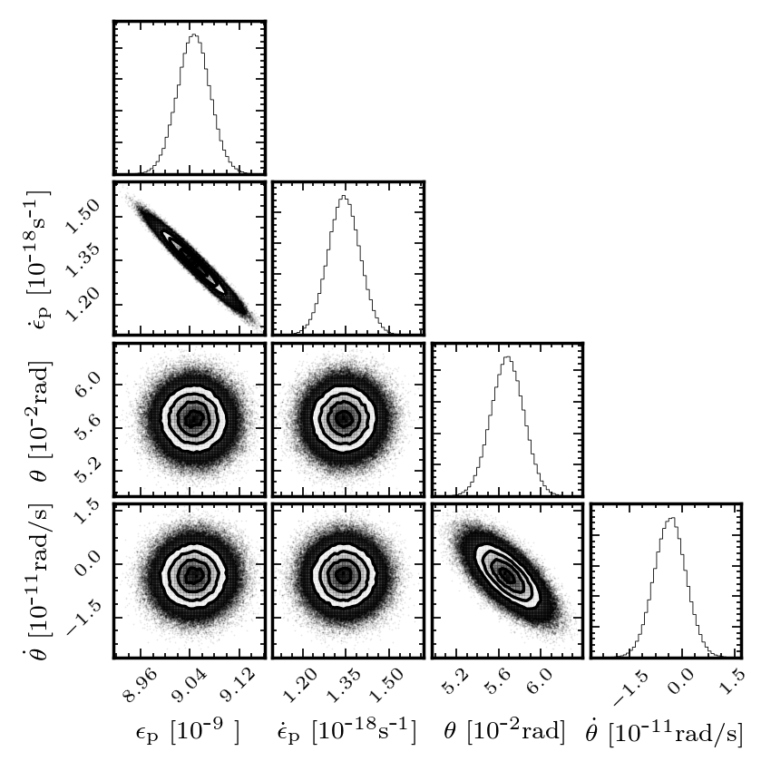
Figure 7: Posterior probability distributions for the wobble angle $\theta$, the deformation $\epsilon_{\mathrm{p}}$ and their rates of change in the $\{\dot{\theta},\dot{\epsilon}_{\mathrm{p}}\}$-model.

Table 5: Prior distributions and a posterior distribution summary for the $\{\dot{\theta},\dot{\epsilon}_{\mathrm{p}}\}$-model parameters.

	Prior	Posterior median $\pm$ s.d.	Units
$\nu_{0}$	$\mathcal{N}$(2.46887171470, ${7.0}{\times}10^{\textrm{-}11}$)	2.47$\pm$${7.0}{\times}10^{\textrm{-}11}$	Hz
$\dot{\nu}_{0}$	$\mathcal{N}$(${\text{{-}}3.658728}{\times}10^{\textrm{-}13}$, ${5.0}{\times}10^{\textrm{-}19}$)	${\text{{-}}3.66}{\times}10^{\textrm{-}13}$$\pm$${4.9}{\times}10^{\textrm{-}19}$	Hz/s
$\ddot{\nu}_{0}$	$\mathcal{N}$(${8.72}{\times}10^{\textrm{-}25}$, ${9.0}{\times}10^{\textrm{-}27}$)	${8.75}{\times}10^{\textrm{-}25}$$\pm$${8.9}{\times}10^{\textrm{-}27}$	Hz/s2
$\epsilon_{\mathrm{p}}$	$|\mathcal{N}$(0, ${1}{\times}10^{\textrm{-}8}$)$|$	${9.05}{\times}10^{\textrm{-}9}$$\pm$${2.7}{\times}10^{\textrm{-}11}$
$\dot{\epsilon}_{\mathrm{p}}$	$|\mathcal{N}$(0, ${2}{\times}10^{\textrm{-}18}$)$|$	${1.34}{\times}10^{\textrm{-}18}$$\pm$${5.6}{\times}10^{\textrm{-}20}$	s${}^{\textrm{-}1}$
$\theta$	Unif(0, 0.1)	0.0568$\pm$0.0015	rad
$\dot{\theta}$	$\mathcal{N}$(0, ${2.2}{\times}10^{\textrm{-}10}$)	${\text{{-}}3.38}{\times}10^{\textrm{-}12}$$\pm$${4.5}{\times}10^{\textrm{-}12}$	rad/s
$\chi$	Unif($2\uppi/5$, $\uppi/2$)	1.5529$\pm$0.0007	rad
$\psi_{0}$	Unif(0, $2\uppi$)	4.7703$\pm$0.0398	rad
$\rho_{2}^{0}$	Unif(0, 0.1464)	0.0236$\pm$0.0004	rad
$\rho_{2}^{\prime\prime}$	$\mathcal{N}$(0, 6.83)	3.25$\pm$0.2	rad${}^{\textrm{-}2}$
$\cos(\iota)$	Unif(-1, 1)	${6.77}{\times}10^{\textrm{-}3}$$\pm$${1.3}{\times}10^{\textrm{-}3}$
$\sigma_{\dot{\nu}}$	Unif(0, ${1}{\times}10^{\textrm{-}15}$)	${2.57}{\times}10^{\textrm{-}16}$$\pm$${1.2}{\times}10^{\textrm{-}17}$	$\mathrm{s}^{\textrm{-}2}$
$\sigma_{W_{10}}$	Unif(0, ${5.0}{\times}10^{\textrm{-}3}$)	${1.47}{\times}10^{\textrm{-}3}$$\pm$${4.0}{\times}10^{\textrm{-}5}$	s

Figure 8 shows the resulting posterior for the timescale of $\theta$-evolution, $\tau_{\theta}=|\theta/\dot{\theta}|$.

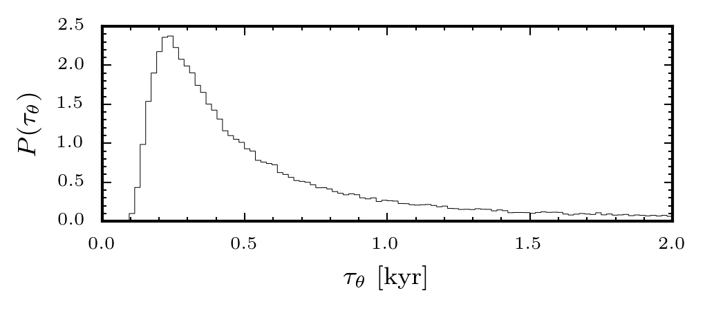
Figure 8: The posterior distribution for the $\theta$-evolution timescale $\tau_{\theta}=|\theta/\dot{\theta}|$ under the $\{\dot{\theta},\dot{\epsilon}_{\mathrm{p}}\}$-model.

We see that the tighter posterior on $\dot{\theta}$ shifts the probability of $\tau_{\theta}$ to larger values than those seen in Figure 4, favouring slower rates of change of $\theta$.

We can place a 95% credible lower limit of $\tau_{\theta}>170.9\,\mathrm{years}$ and the distribution has a median value of $450.2\,\mathrm{years}$. In this combined model, $\tau_{\epsilon}=213\pm 10\,\mathrm{years}$ (the timescale remains unchanged from the $\dot{\epsilon}_{\mathrm{p}}$-model considered in section 6).

We obtain the odds in favour of the $\{\dot{\theta},\dot{\epsilon}_{\mathrm{p}}\}$-model compared to the base-model as $10^{72.45\pm 0.96}$, i.e. slightly less than for the $\dot{\epsilon}_{\mathrm{p}}$-model. We see that, similarly to the case of the $\dot{\theta}$-model, the introduction of $\dot{\theta}$ does not produce a significant-enough improvement in the fit compared to the increase in prior volume.

8 Discrete jumps in deformation: the $\Delta\epsilon_{\mathrm{p}}$-model

The success of the $\dot{\epsilon}_{\mathrm{p}}$-model of section 6 indicates that a time-dependent $\epsilon_{\mathrm{p}}(t)$ provides a significant improvement over the base-model. In this section, we explore an alternative to the slow secular change by modelling the time-variation as a set of discrete jumps in $\epsilon_{\mathrm{p}}$.

8.1 Defining the $\Delta\epsilon_{\mathrm{p}}$-model

In this model extension, we allow $\epsilon_{\mathrm{p}}$ to undergo $N$ distinct positive jumps. For each jump $j\in[1,\,N]$ at time $t_{j}$, we define two dimensionless parameters: the fractional observation time at which the jump occurs, $R_{j}\equiv(t_{j}-t_{0})/T_{\mathrm{obs}}\in[0,1]$, where $t_{0}$ is the start-time and $T_{\mathrm{obs}}$ is the total observation time, and the fractional (positive) variation in $\epsilon_{\mathrm{p}}$ at the jump, $\Delta_{j}\equiv\Delta\epsilon_{\mathrm{p},j}/\epsilon_{\mathrm{p},0}\in[0,\infty)$. In this way, the time evolution of $\epsilon_{\mathrm{p}}(t)$ can be written as

$$\epsilon_{\mathrm{p}}(t)=\epsilon_{\mathrm{p},0}\,\left(1+\sum_{j=1}^{N}H(t-t_{0}-R_{j}\,T_{\mathrm{obs}})\,\Delta_{j}\right),$$ (18)

where $H(t)$ is the Heaviside step function.

8.2 Applying the $\Delta\epsilon_{\mathrm{p}}$-model to the data

We assign a uniform prior distribution over the total observation span for $R_{j}$, the time of the jumps, with $R_{j}<R_{j+1}\;\forall\;j$. For the jump sizes $\Delta_{j}$ we will use a prior consistent with the $\dot{\epsilon}_{\mathrm{p}}$-model (see section 6), specifically a zero-mean Gaussian for $\dot{\epsilon}_{\mathrm{p}}$ with standard-deviation of $2\times 10^{-18}$ s^-1. Distributing an equivalent total change in $\epsilon_{\mathrm{p}}$ on $N$ discrete jumps, this gives an approximate scale of

$$\Delta\approx\frac{\dot{\epsilon}_{\mathrm{p}}\,T_{\mathrm{obs}}}{\epsilon_{\mathrm{p}}\,N}\approx\frac{0.1}{N},$$ (19)

where we have substituted $\epsilon_{\mathrm{p}}$ and $\dot{\epsilon}_{\mathrm{p}}$ for the prior standard-deviation used in the $\dot{\epsilon}_{\mathrm{p}}$-model. We use this to set the scale for a Gaussian prior on the fractional jump size as $\Delta_{j}\sim|\mathcal{N}(0,\,0.1/N)|$.

To speed up the fitting process we have modified the original MCMC fitting process described in Appendix A of Ashton et al. (2016). Specifically, it was found that when fitting for the jump parameters, the MCMC chains took a long time to find the base-model best estimates for the spin-down parameters $\nu_{0}$, $\dot{\nu}_{0}$, and $\ddot{\nu}_{0}$ and the angles $\chi$ and $\theta$. Therefore, instead of initialising the chains from the prior, for the parameters shared with the base-model we initialise them from the base-model posterior. This modification does not change our final estimates, provided that the burn-in period is sufficiently long to allow them to evolve from this point and explore all areas of the parameter space. For several values of $N$, we tested that evolving from the prior produced the same results, but the computation took longer to converge.

The number of jumps $N$ can itself be thought of as a model parameter: ideally we would fit $N$ as part of the MCMC sampling. However, to do this one must use a reversible-jump MCMC algorithm which can vary the number of model dimensions. This is not currently implemented in the software used in this analysis. Instead we have opted for a crude, but sufficient method in which we fit the model for different values of $N$ individually and then use the respective odds to compare them. For each increase in $N$, the number of steps required to reach convergence increases.

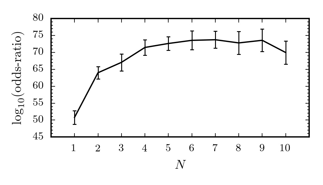
Figure 9: The log odds-ratio for the $\Delta\epsilon_{\mathrm{p}}$-model for a varying number of jumps $N$ compared to the base-model.

In Figure 9 we show the odds of the $N$-jump model compared to the base-model as a function of the number of jumps $N$. We see that up to $N\sim 6$ the odds increase, then reach a plateau and start to marginally decrease for $N=10$.

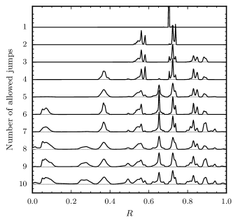
Figure 10: The combined posteriors for the fractional jump times $R$ for the different $N$-jump $\Delta\epsilon_{\mathrm{p}}$-models. The left-hand axis indicates the respective number of jumps $N$. For each $N$, a vertical offset has been added to each posterior to allow them to be distinguished and dashed lines mark the ‘zero’ line.

In Figure 10 we present a stacked plot showing the posteriors on the jump times $R$ for all jumps, for the different $N$-jump models. For ease of reading the plot, each jump is normalised so that the area under the $N=1$ line is 1, under the $N=2$ model the area is 2, etc.

The positions $R$ at which the jumps occur appear consistent between different $N$-jump models. Moreover, the posteriors for each jump are multimodal, each having a unique ‘fingerprint’, which also appear consistent between models. This would not necessarily be expected if the best fit was quite agnostic about the exact jump times and simply distributed $N$ jumps randomly over the observation period. We also see a consistent progression play out as the number of allowed steps $N$ is increased: up to $N=6$ each increase in $N$ finds a new jump site, but from $N\geq 7$ the new jump sites are not so well defined. However, we cannot rule out the possibility that the MCMC chains did not successfully converged for some of these models.

The data does not seem to strongly favour a particular number of jumps above $N\geq 6$. Therefore, for illustrative purposes we will use $N=6$ as our posterior estimate for $N$. While this model does not have the largest odds-ratio (as shown in Figure 9), the difference to the N=7 model, which does have the largest odds-ratio, is much smaller than the error bars. Moreover, this model captures all of the essential features of the discrete jumps as seen in Figure 10.

8.3 The $N=6$ $\Delta\epsilon_{\mathrm{p}}$-model

Figure 11 shows the posterior for the six relative jump sizes $\Delta_{j}$ which have typical sizes of order $\Delta_{j}\sim 0.01$. We provide a summary of the priors and posteriors for all the model parameters in Table 6. Then, in Figure 12 we show the MPE fits to the spin-down and beam-width data; we indicate the jump times with vertical lines. By eye, the fit shows a similar level of improvement compared to the base-model Figure 2 as that observed in Figure 6, which is consistent with the similar odds of $10^{73.53\pm 2.79}$ relative to the base-model. As such we cannot distinguish between the two types of evolving deformation (continuous evolution verses discrete jumps).

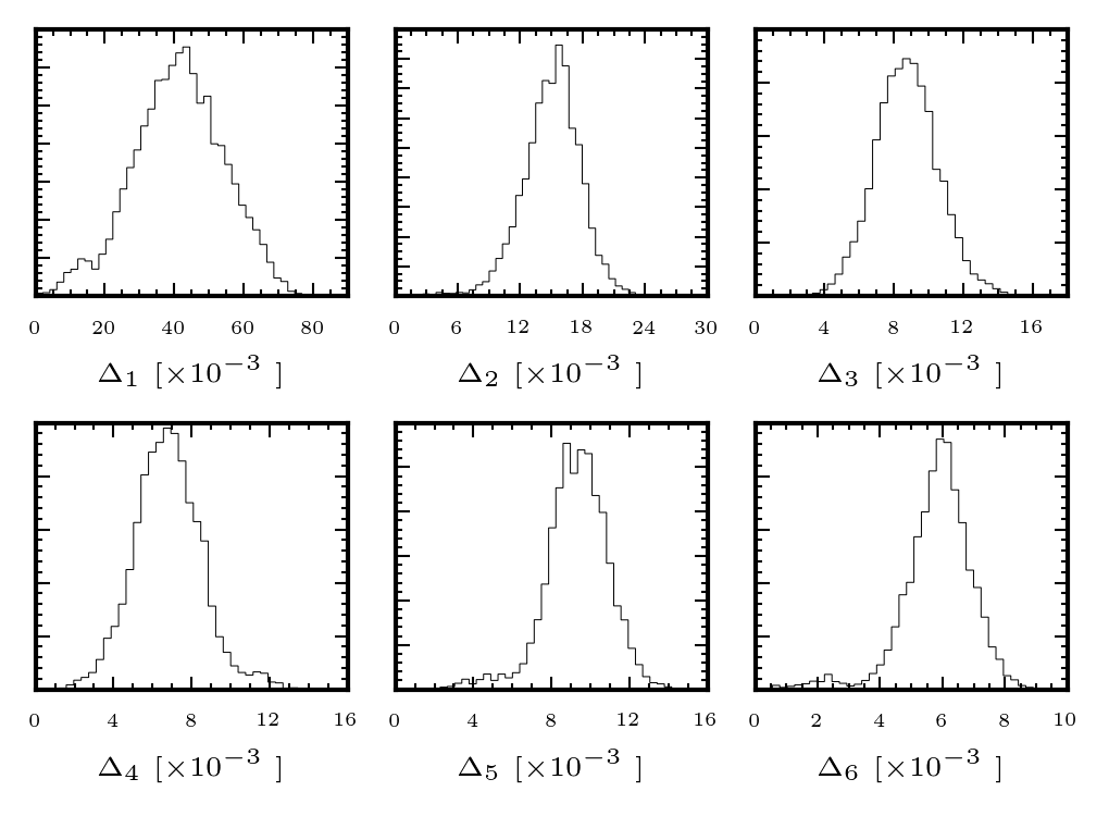
Figure 11: Posterior probability distributions for the six relative jump-size parameters $\Delta_{j}$ in the $\Delta\epsilon_{\mathrm{p}}$-model.

Table 6: Prior distributions and a posterior distribution summary for the $N=6$ $\Delta\epsilon_{\mathrm{p}}$-model parameters.

	Prior	Posterior median $\pm$ s.d.	Units
$\nu_{0}$	$\mathcal{N}$(2.46887171470, ${7.0}{\times}10^{\textrm{-}11}$)	2.47$\pm$${7.2}{\times}10^{\textrm{-}11}$	Hz
$\dot{\nu}_{0}$	$\mathcal{N}$(${\text{{-}}3.658728}{\times}10^{\textrm{-}13}$, ${5.0}{\times}10^{\textrm{-}19}$)	${\text{{-}}3.66}{\times}10^{\textrm{-}13}$$\pm$${4.7}{\times}10^{\textrm{-}19}$	Hz/s
$\ddot{\nu}_{0}$	$\mathcal{N}$(${8.72}{\times}10^{\textrm{-}25}$, ${9.0}{\times}10^{\textrm{-}27}$)	${8.75}{\times}10^{\textrm{-}25}$$\pm$${8.6}{\times}10^{\textrm{-}27}$	Hz/s2
$\epsilon_{\mathrm{p}}$	$|\mathcal{N}$(0, ${1}{\times}10^{\textrm{-}8}$)$|$	${8.82}{\times}10^{\textrm{-}9}$$\pm$${1.4}{\times}10^{\textrm{-}10}$
$\Delta_{1}$	$|\mathcal{N}$(0, 0)$|$	0.04$\pm$0.0
$R_{1}$	Unif(0, 1)	0.07$\pm$0.0
$\Delta_{2}$	$|\mathcal{N}$(0, 0)$|$	0.02$\pm$${2.8}{\times}10^{\textrm{-}3}$
$R_{2}$	Unif(0, 1)	0.37$\pm$0.0
$\Delta_{3}$	$|\mathcal{N}$(0, 0)$|$	${8.71}{\times}10^{\textrm{-}3}$$\pm$${1.8}{\times}10^{\textrm{-}3}$
$R_{3}$	Unif(0, 1)	0.55$\pm$0.0
$\Delta_{4}$	$|\mathcal{N}$(0, 0)$|$	${6.76}{\times}10^{\textrm{-}3}$$\pm$${1.7}{\times}10^{\textrm{-}3}$
$R_{4}$	Unif(0, 1)	0.65$\pm$0.0
$\Delta_{5}$	$|\mathcal{N}$(0, 0)$|$	${9.37}{\times}10^{\textrm{-}3}$$\pm$${1.7}{\times}10^{\textrm{-}3}$
$R_{5}$	Unif(0, 1)	0.73$\pm$0.0
$\Delta_{6}$	$|\mathcal{N}$(0, 0)$|$	${5.94}{\times}10^{\textrm{-}3}$$\pm$${1.1}{\times}10^{\textrm{-}3}$
$R_{6}$	Unif(0, 1)	0.85$\pm$0.0
$\theta$	Unif(0, 0.1)	0.0572$\pm$0.0011	rad
$\chi$	Unif($2\uppi/5$, $\uppi/2$)	1.5539$\pm$0.0007	rad
$\psi_{0}$	Unif(0, $2\uppi$)	4.7351$\pm$0.0535	rad
$\rho_{2}^{0}$	Unif(0, 0.1464)	0.0233$\pm$0.0003	rad
$\rho_{2}^{\prime\prime}$	$\mathcal{N}$(0, 6.83)	3.33$\pm$0.2	rad${}^{\textrm{-}2}$
$\cos(\iota)$	Unif(-1, 1)	${7.2}{\times}10^{\textrm{-}3}$$\pm$${1.2}{\times}10^{\textrm{-}3}$
$\sigma_{\dot{\nu}}$	Unif(0, ${1}{\times}10^{\textrm{-}15}$)	${2.44}{\times}10^{\textrm{-}16}$$\pm$${1.2}{\times}10^{\textrm{-}17}$	$\mathrm{s}^{\textrm{-}2}$
$\sigma_{W_{10}}$	Unif(0, ${5.0}{\times}10^{\textrm{-}3}$)	${1.44}{\times}10^{\textrm{-}3}$$\pm$${3.9}{\times}10^{\textrm{-}5}$	s

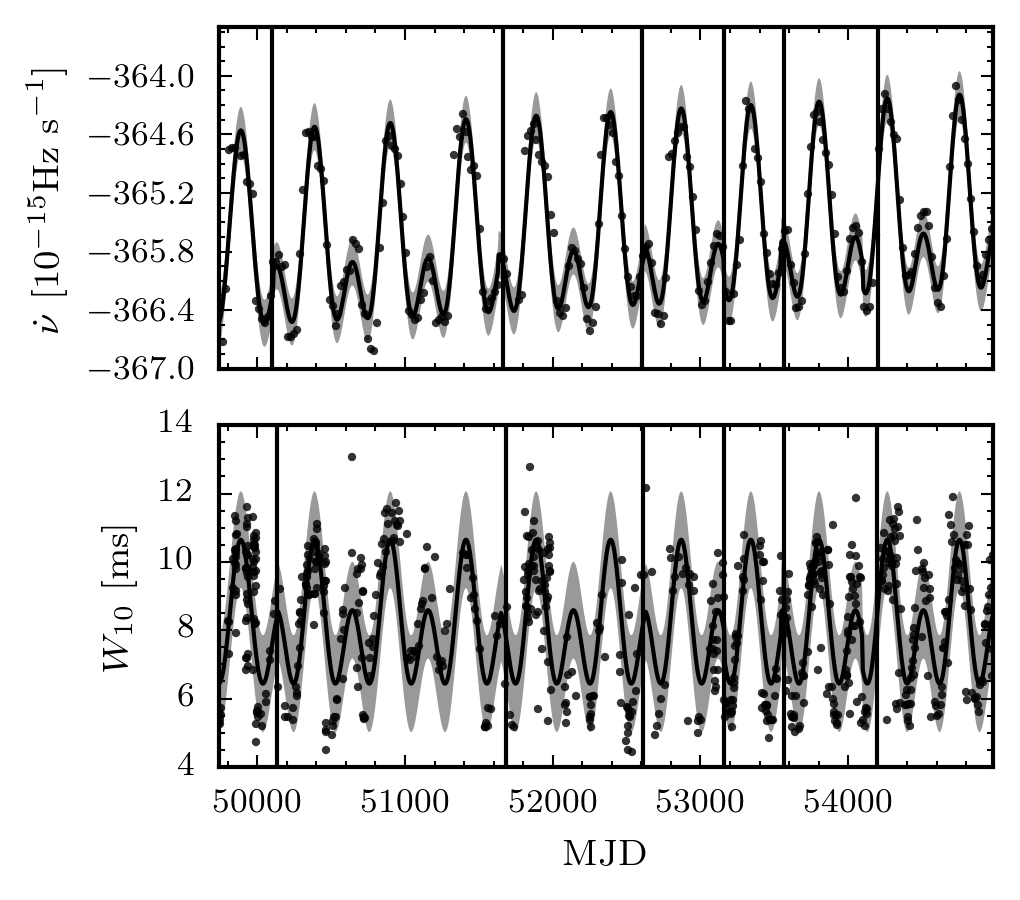
Figure 12: Comparison between the MPE $\Delta\epsilon_{\mathrm{p}}$-model with $N=6$ jumps (solid line) and the observed spin-down and beam-width data (black dots). Vertical lines mark the times of the six (positive) jumps in $\epsilon_{\mathrm{p}}(t)$. The shaded region indicates the estimated $1\,\sigma$ noise level.

9 Interpreting the upper limit on $\dot{\theta}$

Dissipative processes internal to the star may damp the wobble motion, leading to a decrease in $\theta$. Looking at the posterior on $\dot{\theta}$ shown in Figure 7, we see that, while the peak of the probability distribution lies at a value $\dot{\theta}<0$, the peak is nevertheless close to $\dot{\theta}=0$, so there is no clear evidence for any evolution in the wobble angle over the duration of these observations. Slightly more informatively, in Figure 8 we plotted the posterior on the timescale $\tau_{\theta}=|\theta/\dot{\theta}|$.

Even though this analysis finds no evidence for a secular variation in the wobble angle, we can use these results to put a lower bound on the timescale on which $\tau_{\theta}$ evolves, i.e. we can place a 95% credible interval that $\tau_{\theta}>170.9$ years.

Mutual friction, a dissipative coupling of neutron vortices and the charged component of the star, is the leading candidate for damping precession. The effect of mutual friction on precession was examined by Sedrakian et al. (1999) and Glampedakis et al. (2008, 2009). The strength of the interaction can be parameterised by a dimensionless quantity $\mathcal{R}$, a measure of the relative strength of the mutual friction force to the Magnus force. In the limit of large $\mathcal{R}$, the vortices become pinned to the crust, and a very fast precession frequency is obtained, in contradiction with the observations. The free precession observation instead requires the weak drag limit, $\mathcal{R}\ll 1$, to apply. The damping time can be shown to be given by

$$\tau_{\rm MF}=\frac{1}{{\cal R}\epsilon_{\mathrm{p}}2\uppi\nu}\frac{I_{\rm prec}}{I_{\rm SF}},$$ (20)

where $I_{\rm SF}$ denotes the moments of inertia of the core superfluid (see Sedrakian et al. (1999) and Appendix A of Glampedakis et al. (2009)). Strictly, $\cal R$ is a locally-defined quantity, i.e. a function of density, but this dependence is ‘averaged-out’ in the rigid-body dynamics analysis through which the above equation is obtained.

Given that the value of $\epsilon_{\mathrm{p}}$ is known from our posterior estimate, we can, as described in Glampedakis et al. (2009), convert our lower bound on $\tau_{\theta}$ to a 95% credible upper bound on $\cal R$ assuming that $\tau_{\theta}=\tau_{\rm MF}$:

$${\cal R}\lesssim 1.2{\times}10^{-4}\left(\frac{170.9\,\rm yr}{\tau_{\theta}}\right)\left(\frac{9.7{\times}10^{-9}}{\epsilon_{\mathrm{p}}}\right)\left(\frac{I_{\rm prec}/I_{\rm SF}}{0.1}\right).$$ (21)

Again as noted in Glampedakis et al. (2009), this can be combined with a lower bound on $\cal R$ that comes from analysis of the Christmas 1988 glitch in the Vela pulsar, where the relevant coupling time can be shown to be given by $\tau_{\rm MF}=1/(4\uppi\nu{\cal R})I_{\rm prec}/I_{\rm SF}$. From the analysis of the Vela glitch by Abney et al. (1996), if we set $I_{\rm prec}/I_{\rm SF}=0.1$, we obtain $30$ seconds as the upper limit on the crust-core coupling timescale, leading to a lower bound ${\cal R}\gtrsim 2.4\times 10^{-5}$. Combining these results, we have

$$2.4\times 10^{-5}\lesssim{\cal R}\lesssim 1.2\times 10^{-4}.$$ (22)

The upper limit given here is an improvement by about one order of magnitude on that given by Glampedakis et al. (2009).

A number of authors have attempted first-principles microphysical calculations of this parameter, appropriate for a neutron superfluid core (Alpar et al., 1984; Alpar & Sauls, 1988; Andersson et al., 2006). Taking Equation (64) of Andersson et al. (2006), and setting the density $10^{14}$ g cm^-3, and the proton density fraction to $0.1$, one obtains a range for ${\cal R}\approx 9.7\times 10^{-5}$–$3.18\times 10^{-4}$ as one varies the proton effective mass over the interval $0.5$–$0.7$ times the bare mass. Clearly, there is a reasonable level of convergence between the shrinking observation range in $\cal R$ reported above and microscopic estimates.

10 Interpreting the evolving deformation

The rather rapid observed decrease in the free precession period is not easy to explain within the precessional model. We have shown above that it corresponds to an increase in the deformation parameter $\epsilon_{\mathrm{p}}$ of Equation (missing) 5. Re-writing this slightly,

$$\epsilon_{\mathrm{p}}=\frac{\Delta I_{\rm d}}{I_{\rm prec}}=\frac{\Delta I_{\rm d}}{I_{*}}\frac{I_{*}}{I_{\rm prec}},$$ (23)

we see that we can interpret our observation as an increase on the deformation $\Delta I_{\rm d}/I_{*}$, and/or a decrease in the fraction of the star that participates in the free precession, $I_{\rm prec}/I_{*}$. The total variation must correspond to a timescale of $\approx 213$ years, a rather short timescale for a $\sim 10^{5}$ year old neutron star.

It is difficult to motivate a variation in $I_{\rm prec}/I_{*}$ on this sort of timescale. One possible mechanism for producing a decrease in this quantity would be if the core superfluid does not contribute to $I_{\rm prec}$. Then, if the star is currently cooling through the density-dependent normal matter–superfluid matter transition, the amount of core superfluid matter will be gradually increasing, with a corresponding decrease in the amount of core normal matter, hence, by our current assumption, decreasing $I_{\rm prec}$. Such a mechanism has been used by Ho & Andersson (2012) to explain the $n<3$ braking indices in some young pulsars. However, it is difficult to countenance such a mechanism applying here. PSR B1828-11 is a relatively old pulsar, and probably cooled through the normal fluid/superfluid transition when it was much younger. Also, its observed braking index is $n\approx 16$ (see Table Table 1), so does not have $n<3$ as would be expected if the electromagnetic spin-down torque were acting on a progressively smaller fraction of the stellar moment of inertia. Also, in the model of Ho & Andersson (2012), the newly created superfluid is required to pin to the crust, something which would result in a much more rapid rise in the free precession frequency via the gyroscopic effect of a pinned superfluid in a rotating star (Shaham, 1977)–see the discussion below.

The alternative possibility is that the deformation $\Delta I_{\rm d}/I_{*}$ is steadily increasing. The deformation itself may be supported by elastic and/or magnetic strains. In the case of elastic strains, it is very difficult to understand why the deformation should increase with time. Elastic strains can be expected to be steadily reduced by plastic flow (and possibly by occasional crustquakes), which would lead to a decreasing deformation.

In the case of magnetically-sustained deformations, it is again puzzling that the deformation should increase with time, as magnetic fields can be expected to decay, although the interplay of Ohmic decay, Hall drift and ambipolar diffusion processes can lead to a complicated evolution, with the (local) field strength increasing in some places. Nevertheless, the required evolution timescale $\sim 200$ years is short compared to the timescales expected for these processes (see e.g. Goldreich & Reisenegger (1992)).

Note that if the exterior magnetic field also evolves on this time scale, then we should be able to measure it from the braking index. That is we allow $B{=}B(t)$ in the usual vacuum dipole braking law (Shapiro & Teukolsky, 1983) and solve for the derived braking index, giving

$$n=\frac{\ddot{\nu}\nu}{\dot{\nu}^{2}}=3+2\frac{\tau_{\mathrm{age}}}{\tau_{B}}\approx 10^{3}\left(\frac{\tau_{\mathrm{age}}}{10^{5}\;\mathrm{yrs}}\right)\left(\frac{\tau_{B}}{200\;\mathrm{yrs}}\right)^{-1}.$$ (24)

This is much larger than the measured value of $n\approx 16$ (see Table 1). So we can exclude models where the exterior field evolves in tandem with the internal one, but it remains unclear if the internal field could vary on such a timescale.

The possibility of the star containing a pinned superfluid component adds an additional strand to this story. As shown by Shaham (1977), a pinned superfluid has a profound effect on the precession frequency, adding a term proportional to $I_{\rm PSF}$, the amount of pinned superfluid:

$$\frac{P}{P_{\rm fp}}=\frac{\Delta I_{\rm d}}{I_{\rm prec}}+\frac{I_{\rm PSF}}{I_{\rm prec}},$$ (25)

valid for small wobble angle and with the pinning directed along the symmetry axis of the biaxial star. Assuming that the quantity $\Delta I_{\rm d}/I_{\rm prec}$ is positive (or else negligible), this immediately translates into the bound $I_{\rm PSF}/I_{\rm prec}\lesssim 10^{-8}$ for PSR B1828-11, much less than the value expected on the basis of microphysical considerations and superfluid glitch theory (Jones & Andersson, 2001; Link & Epstein, 2001). A possible explanation for this has been advanced by Link & Cutler (2002), who argued that the precessional motion itself might cause most/all of the pinning to break.

This has motivated most models of PSR B1828-11 assuming that $I_{\rm PSF}$ is exactly zero. However, as noted above, a small amount of pinning is allowed. This suggests an alternative mechanism to explain the evolving precession period: the previously broken pinning may be gradually re-establishing itself, with the amount of pinned superfluid increasing steadily over the last $\sim 200$ years. Indeed, we can estimate the timescale $\Delta t_{\textrm{re-pin}}$ for the gradual re-pinning to re-establish a reservoir of pinned superfluid of moment of inertia $\Delta t_{\textrm{re-pin}}$. From Equation (missing) 25 we have $\dot{I}_{\rm PSF}=I_{\rm prec}\dot{\epsilon}_{\rm p}$, so

$$\Delta t_{\textrm{re-pin}}=\frac{\Delta I_{\textrm{re-pin}}}{\dot{I}_{\rm PSF}}=2.13\times 10^{8}{\,\rm yr}\,\,\,\frac{\Delta I_{\textrm{re-pin}}/I_{*}}{10^{-2}}\frac{I_{*}}{I_{\rm prec}},$$ (26)

implying that such unpinning events have to be rare in the pulsar population, as PSR B1828-11 will not build up a typically sized pinned superfluid reservoir (at the few percent level) for a long time to come.

The ideas discussed here (evolving strain and pinned superfluidity) are all relevant to the physics of pulsar glitches. In fact, PSR B1828-11 was observed to glitch in 2009: see Espinoza et al. (2011) and www.jb.man.ac.uk/~pulsar/glitches/gTable.html). The interplay between the modelling of the free precession and the glitch is an interesting topic in its own right. We have explored the consistency requirements between the free precession interpretation of the observed quasi-periodicities and glitches in a separate publication (Jones et al., 2016), which exposes significant tensions between the small wobble angle free precession model considered here and standard models of pulsar glitches.

11 Discussion & Outlook

In this work, we have extended the free precession model of Ashton et al. (2016) to allow for both the wobble angle $\theta$ and the deformation $\Delta I_{\rm d}/I_{\rm prec}$ of PSR B1828-11 to evolve in time. The generalisation to allow for $\theta$ to vary was extremely natural, as dissipative processes internal to the star are expected to affect the wobble angle, causing it to decay in oblate stars ($\Delta I_{\rm d}>0$), and grow in prolate ones ($\Delta I_{\rm d}<0$; (Cutler, 2002)). That the deformation $\Delta I_{\rm d}/I_{\rm prec}$ should vary in time is less obvious. However, we first showed, in a completely model independent way (i.e. independently of the cause of the quasi-periodic oscillation in spin-down rate) that the $\sim 500$ day modulation period was getting shorter; this necessitated the allowance for a time-varying deformation in our precession model.

We in fact found no evidence for a variation in the wobble angle, with the inclusion of this new effect not producing a significant improvement in our ability to fit the data. We therefore proceeded to set an upper limit on the timescale on which it varied, $\tau_{\theta}\gtrsim 171$ years. We translated this into an upper bound on the strength of the mutual frictional parameter ${\cal R}\lesssim 1.2\times 10^{-4}$, describing the strength of the coupling between the crust and core, improving on previously published results by approximately one order of magnitude. When combined with a lower limit on the strength of this coupling, as deduced previously by analysis of the Vela 1988 glitch, this parameter is confined to the interval $2.4\times 10^{-5}\lesssim{\cal R}\lesssim 1.2\times 10^{-4}$, a rather narrow range, but consistent with microscopic calculation.

In terms of the evolving deformation, we explored two phenomenological ways to model this: either as a smooth secular evolution of the deformation or as $N$ discrete jumps in the deformation. We find that both of these models produce a substantial improvement in the fit when compared to the base-model—decisive evidence that, in the context of precession, the magnitude of the star’s deformation is growing; this can be seen in Table 7 where we list the odds-ratios for all models extensions considered in this work. For the discrete jumps model discussed in section 8, we found $6$ or more jumps seemed to produce the best fit and used the $N=6$ model to illustrate our results.

Table 7: The log odds-ratio for all tested models against the base-model.

Model	$\log_{10}(\mathrm{odds-ratio})$
$\dot{\theta}$	$-1.70\pm 1.39$
$\dot{\epsilon}_{\mathrm{p}}$	$73.65\pm 0.97$
$\{\dot{\theta},\dot{\epsilon}_{\mathrm{p}}\}$	$72.45\pm 0.96$
N=6 $\Delta\epsilon_{\mathrm{p}}$	$73.53\pm 2.79$

The odds-ratio between the $\dot{\epsilon}_{\mathrm{p}}$-model and the N=6 $\Delta\epsilon_{\mathrm{p}}$-model is $10^{0.11\pm 2.87}$, so we find no evidence to favour one of these two evolution models over the other. For both models an approximately equivalent informative prior was used, but when the odds-ratio is marginal the prior can have a substantial effect. We therefore cannot state without further investigation which of the two model extensions is preferred with certainty and without unfounded bias from the prior. It would be useful to propose substantive physical models which have well defined priors; this would allow a more thorough statement to be made.

We discussed the possible physical cause of the evolution in the deformation. We mentioned elastic, magnetic and pinned superfluid interpretations, and pointed out some difficulties with all of these. PSR B1828-11 underwent a glitch in 2009 (Espinoza et al., 2011). In a separate publication, we discuss consistency requirements between the precession model described here and the glitch, folding in the evolving precession period into our discussion (Jones et al., 2016).

In interpreting this changing deformation, it may be important to note that while in this analysis we fitted the ‘small-$\chi$’ model (as defined by Arzamasskiy et al. (2015)), our analysis can equally be applied to the ‘large-$\chi$’ model by interchange of the $\theta$ and $\chi$ labels at the parameter estimation stage. This is shown in Appendix A and is due to the symmetry in $\theta$ and $\chi$ in the spin-down and beam-width models. The two solutions correspond to quite different physical scenarios which may result in fundamental differences in their interpretation.

The findings presented in this work provide a new way to probe neutron star physics. It remains to be understood what is the true cause of the changing deformation and whether this happens as a smooth secular evolution or as a number of discreet jumps. Moreover, it would be interesting to know if alternative models to precession can better model this behaviour.

Appendix A Derivation of the spin-down rate and the $\theta\leftrightarrow\chi$ symmetry

In this appendix, we derive the spin-down rate for a precessing pulsar under a vacuum point-dipole spin-down torque. We will use a generalisation of vacuum point-dipole torque to allow for a braking index $n\neq 3$, but retain the angular dependence.

Following Section 6.1.1 of Jones & Andersson (2001), let $\Theta$ be the polar angles made by the magnetic dipole with respect to the $z$-axis in the inertial frame and $\Phi$ be the azimuthal angle with respect to the $x-z$ axes. Then our generalisation of the vacuum point-dipole spin-down torque can be written as

$$\ddot{\Phi}=-k\dot{\Phi}^{n}\sin^{2}\Theta,$$ (27)

where $k$ is a positive constant. Rearranging Equation (missing) 7 and expanding about $\theta=0$ up to $\mathcal{O}(\theta^{2})$, we find

$$\begin{split}\sin^{2}\Theta=&\sin^{2}\Theta_{0}-2\theta\sin\chi\cos\chi\sin\psi(t)\\ &+\frac{1}{2}\theta^{2}\sin^{2}\chi\cos(2\psi(t)),\end{split}$$ (28)

where we have defined

$$\sin^{2}\Theta_{0}\equiv\sin^{2}\chi+\theta^{2}\left(\cos^{2}\chi-\frac{\sin^{2}\chi}{2}\right),$$ (29)

a constant, while the second two terms in Equation (missing) 28 provide the first and second harmonic modulations in $\sin^{2}\Theta$.

In order to find approximate solutions to Equation (missing) 27, we begin by substituting the $\sin^{2}\Theta$ in Equation (missing) 27 with the time-averaged constant $\sin^{2}\Theta_{0}$ value and solve to get

$$\dot{\Phi}(t)=\dot{\Phi}_{0}\left[1+(n-1)\frac{t}{\tau_{\mathrm{age}}}\right]^{\frac{-1}{n-1}},$$ (30)

where

$$\tau_{\mathrm{age}}=\frac{|\dot{\Phi}_{0}|}{|\ddot{\Phi}_{0}|}\approx\frac{1}{k|\dot{\Phi}_{0}|^{(n-1)}\sin^{2}\Theta_{0}}.$$ (31)

Now, we substitute Equation (missing) 30 back into Equation (missing) 27 along with the expanded, but complete variation in $\sin^{2}\Theta$. To simplify the result, we expand in $t/\tau_{\mathrm{age}}\ll 1$ and write the result in terms of the spin frequency and its derivatives as

$$\dot{\nu}(t)=\dot{\nu}_{0}+\ddot{\nu}_{0}t-\dot{\nu}_{0}\theta\left[2\cot\chi\sin\psi(t)-\frac{1}{2}\theta\cos(2\psi(t))\right]$$ (32)

In this derivation, we make no assumptions on how $\psi(t)$ evolves. However, since we are interested in cases where $\tau_{\mathrm{P}}\ll\tau_{\mathrm{age}}$ we will assume that

$$\psi(t)=\dot{\psi}t+\psi_{0}.$$ (33)

Then, following Sec 3 of Jones & Andersson (2001), but retaining the dependence on $\theta$, we can write this as

$$\psi(t)=-2\uppi\frac{t}{\tau_{\mathrm{P}}}+\psi_{0}.$$ (34)

where

$$\tau_{\mathrm{P}}\equiv\frac{1}{\epsilon_{\mathrm{p}}\nu(t)\cos\theta}$$ (35)

It can be shown that deriving this expression, but making the assumption $\chi\ll 1$ in Equation (missing) 28 and throughout (rather than $\theta\ll 1$) is equivalent to the transformation $\theta\leftrightarrow\chi$ in Equation (missing) 32. This symmetry was discussed by Arzamasskiy et al. (2015) and fundamentally results from the symmetry of $\theta$ and $\chi$ in Equation (missing) 7. Because the same symmetry also exists in our beam-width model (Equation (missing) 8), the large-$\chi$ solutions presented in this work, can equally be interpreted as small-$\chi$ solutions by interchanging $\theta$ and $\chi$.

Appendix B Consistency of posterior estimates in the $\dot{\epsilon}_{\mathrm{p}}$-model

For the base and $\dot{\epsilon}_{\mathrm{p}}$-model, we investigated the behaviour when conditioned on each data set (spin-down and beam-width) individually in addition to the combined results presented in section 6 and found that both data sets independently support the $\dot{\epsilon}_{\mathrm{p}}$-model over the base-model. In Figure 13 we plot the posteriors for the $\dot{\epsilon}_{\mathrm{p}}$-model parameters that are common to both the spin-down and beam-width parts of the model, excluding the frequency and spin-down parameters which are dominated in all cases by the astrophysical prior.

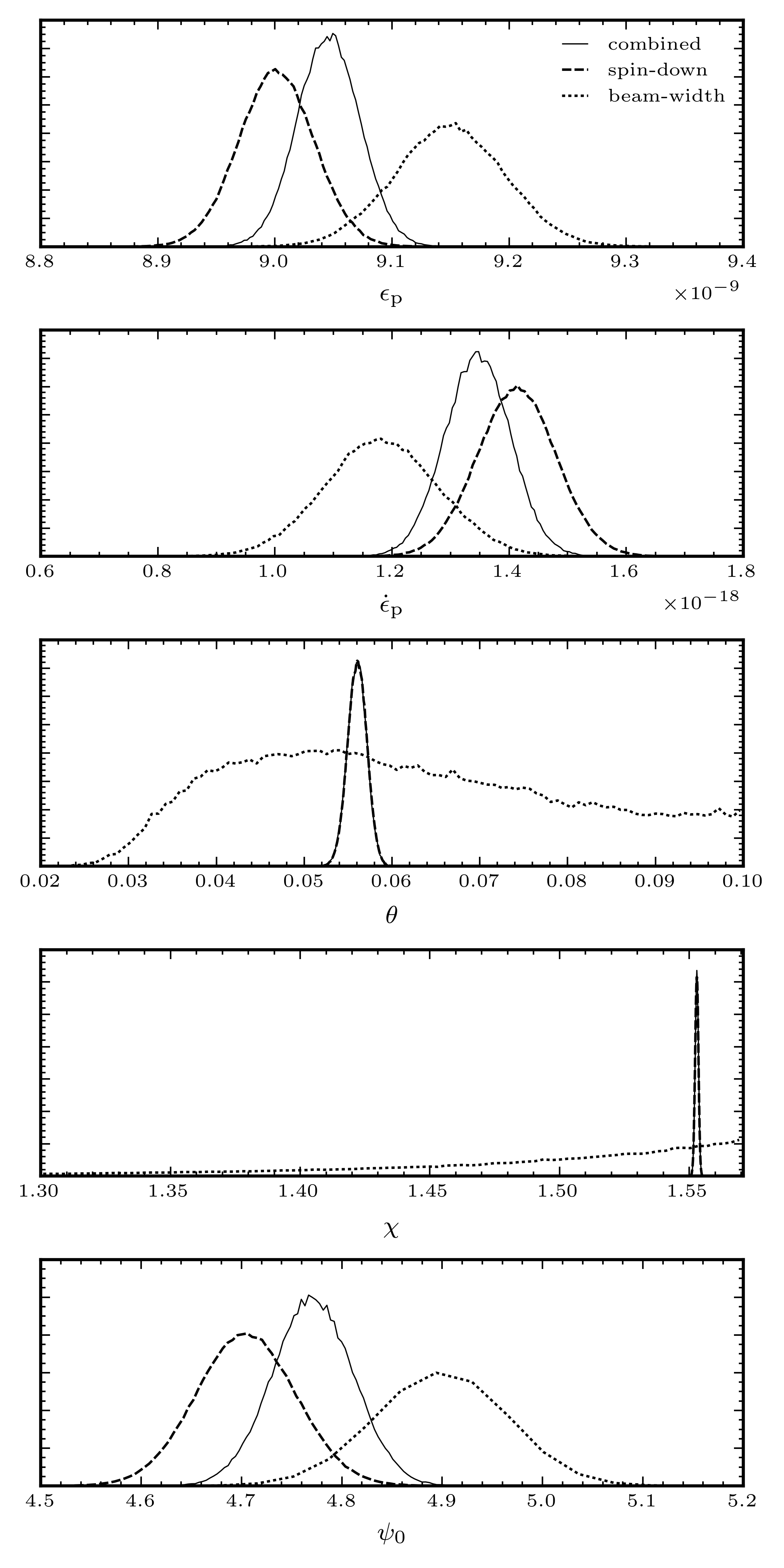
Figure 13: Selected posterior distributions in the $\dot{\epsilon}_{\mathrm{p}}$-model as conditioned on the spin-down and beam-width data individually and the two combined. Note that the $\theta$ and $\chi$ posteriors conditioned on the beam-width data have been scaled by a factor of 10 so that they are visible on the same scale as the strongly peaked spin-down and combined results.

This figure demonstrates that the analysis performed on the two individual data sets independently arrive at reasonably consistent posterior distributions for these shared model parameters, with non-negligible overlap between the posteriors.

For the two angles $\theta$ and $\chi$ the beam-width data does little to constrain the posteriors, with the results even railing against the prior boundaries. Widening the prior (when conditioning on the beam-width) solves this issue, but the posteriors remain uninformative. Comparing with the analysis of the combined data set, we see that the combined posteriors are either a compromise of the individual posteriors, when they are both informative, as is the case for $\epsilon_{\mathrm{p}}$, $\dot{\epsilon}_{\mathrm{p}}$, and $\psi_{0}$, or they are dominated by the more informative spin-down data, as is the case for $\theta$ and $\chi$. As such, when using a combined data set, there is no “tension” (i.e. the two data sets preferring different solutions) and so their log-odds sum approximately to the log-odds of the combined data set.

References

- Abney et al. (1996) Abney M., Epstein R. I., Olinto A. V., 1996, ApJ, 466, L91
- Akgün et al. (2006) Akgün T., Link B., Wasserman I., 2006, MNRAS, 365, 653
- Alpar & Sauls (1988) Alpar M. A., Sauls J. A., 1988, ApJ, 327, 723
- Alpar et al. (1984) Alpar M. A., Langer S. A., Sauls J. A., 1984, ApJ, 282, 533
- Andersson et al. (2006) Andersson N., Sidery T., Comer G. L., 2006, MNRAS, 368, 162
- Arzamasskiy et al. (2015) Arzamasskiy L., Philippov A., Tchekhovskoy A., 2015, MNRAS, 453, 3540
- Ashton et al. (2016) Ashton G., Jones D. I., Prix R., 2016, MNRAS, 458, 881
- Bailes et al. (1993) Bailes M., Lyne A. G., Shemar S. L., 1993, in Phillips J. A., Thorsett S. E., Kulkarni S. R., eds, Astronomical Society of the Pacific Conference Series Vol. 36, Planets Around Pulsars. pp 19–30
- Beaugé et al. (2003) Beaugé C., Ferraz-Mello S., Michtchenko T. A., 2003, ApJ, 593, 1124
- Bisnovatyi-Kogan et al. (1990) Bisnovatyi-Kogan G. S., Mersov G. A., Sheffer E. K., 1990, Soviet Ast., 34, 44
- Cordes (2013) Cordes J. M., 2013, ApJ, 775, 47
- Cutler (2002) Cutler C., 2002, Phys. Rev. D, 66, 084025
- Espinoza et al. (2011) Espinoza C. M., Lyne A. G., Stappers B. W., Kramer M., 2011, MNRAS, 414, 1679
- Foreman-Mackey et al. (2013) Foreman-Mackey D., Hogg D. W., Lang D., Goodman J., 2013, PASP, 125, 306
- Foreman-Mackey et al. (2014) Foreman-Mackey D., Price-Whelan A., Ryan G., Emily Smith M., Barbary K., Hogg D. W., Brewer B. J., 2014, triangle.py v0.1.1, doi:10.5281/zenodo.11020, http://dx.doi.org/10.5281/zenodo.11020
- Glampedakis et al. (2008) Glampedakis K., Andersson N., Jones D. I., 2008, Physical Review Letters, 100, 081101
- Glampedakis et al. (2009) Glampedakis K., Andersson N., Jones D. I., 2009, MNRAS, 394, 1908
- Goggans & Chi (2004) Goggans P. M., Chi Y., 2004, in AIP Conference Proceedings. pp 59–66
- Goldreich & Reisenegger (1992) Goldreich P., Reisenegger A., 1992, ApJ, 395, 250
- Goodman & Weare (2010) Goodman J., Weare J., 2010, Comm. App. Math. Comp. Sci., 5, 65
- Ho & Andersson (2012) Ho W. C. G., Andersson N., 2012, Nature Physics, 8, 787
- Jones (2012) Jones D. I., 2012, MNRAS, 420, 2325
- Jones & Andersson (2001) Jones D. I., Andersson N., 2001, MNRAS, 324, 811
- Jones et al. (2001) Jones E., Oliphant T., Peterson P., et al., 2001, SciPy: Open source scientific tools for Python, http://www.scipy.org
- Jones et al. (2016) Jones D. I., Ashton G., Prix R., 2016, preprint, (arXiv:1610.03509)
- Kramer et al. (2006) Kramer M., Lyne A. G., O’Brien J. T., Jordan C. A., Lorimer D. R., 2006, Science, 312, 549
- Landau & Lifshitz (1969) Landau L. D., Lifshitz E. M., 1969, Mechanics. Pergamon press
- Levin & D’Angelo (2004) Levin Y., D’Angelo C., 2004, ApJ, 613, 1157
- Link (2003) Link B., 2003, Physical Review Letters, 91, 101101
- Link & Cutler (2002) Link B., Cutler C., 2002, MNRAS, 336, 211
- Link & Epstein (2001) Link B., Epstein R. I., 2001, ApJ, 556, 392
- Lyne (2013) Lyne A., 2013, in van Leeuwen J., ed., IAU Symposium Vol. 291, Neutron Stars and Pulsars: Challenges and Opportunities after 80 years. pp 183–188 (arXiv:1212.2250), doi:10.1017/S1743921312023605
- Lyne et al. (2010) Lyne A., Hobbs G., Kramer M., Stairs I., Stappers B., 2010, Science, 329, 408
- Manchester et al. (2005) Manchester R. N., Hobbs G. B., Teoh A., Hobbs M., 2005, AJ, 129, 1993
- Perera et al. (2015) Perera B. B. P., Stappers B. W., Weltevrede P., Lyne A. G., Bassa C. G., 2015, MNRAS, 446, 1380
- Sedrakian et al. (1999) Sedrakian A., Wasserman I., Cordes J. M., 1999, ApJ, 524, 341
- Shaham (1977) Shaham J., 1977, ApJ, 214, 251
- Shapiro & Teukolsky (1983) Shapiro S. L., Teukolsky S. A., 1983, Black Holes, White Dwarfs, and Neutron Stars. John Wiley & Sons, Inc
- Stairs et al. (2000) Stairs I. H., Lyne A. G., Shemar S. L., 2000, Nature, 406, 484
- Stairs et al. (2003) Stairs I. H., Athanasiadis D., Kramer M., Lyne A. G., 2003, in Bailes M., Nice D. J., Thorsett S. E., eds, Astronomical Society of the Pacific Conference Series Vol. 302, Radio Pulsars. p. 249 (arXiv:astro-ph/0211005)
- Townsend (2010) Townsend R., 2010, The Astrophysical Journal Supplement Series, 191, 247
- Wasserman (2003) Wasserman I., 2003, MNRAS, 341, 1020