The Galactic Center Molecular Cloud Survey

We present the first systematic study of the density structure of clouds found in a complete sample covering all major molecular clouds in the Central Molecular Zone (CMZ; inner $\sim{}200\leavevmode\nobreak\ \rm{}pc$) of the Milky Way. This is made possible by using data from the Galactic Center Molecular Cloud Survey (GCMS), the first study resolving all major molecular clouds in the CMZ at interferometer angular resolution. We find that many CMZ molecular clouds have unusually shallow density gradients compared to regions elsewhere in the Milky Way. This is possibly a consequence of weak gravitational binding of the clouds. The resulting relative absence of dense gas on spatial scales $\sim{}0.1\leavevmode\nobreak\ \rm{}pc$ is probably one of the reasons why star formation (SF) in dense gas of the CMZ is suppressed by a factor $\sim{}10$, compared to solar neighborhood clouds. Another factor suppressing star formation are the high SF density thresholds that likely result from the observed gas kinematics. Further, it is possible but not certain that the star formation activity and the cloud density structure evolve systematically as clouds orbit the CMZ.

1 Introduction

The Central Molecular Zone (CMZ) — i.e. the inner $\sim{}200\leavevmode\nobreak\ \rm{}pc$ of our Galaxy — is a star–forming environment with very extreme physical properties. It contains molecular clouds that have unusually high average densities $\gtrsim{}10^{4}\leavevmode\nobreak\ \rm{}cm^{-3}$ on spatial scales of about 1 pc (Sec. 3), are subject to a high confining pressure of $10^{6\leavevmode\nobreak\ {\rm{}to}\leavevmode\nobreak\ 7}\leavevmode\nobreak\ \rm{}K\,cm^{-3}$ (Yamauchi et al., 1990; Spergel & Blitz, 1992; Muno et al., 2004), and are penetrated by strong magnetic fields with strengths $\sim{}5\leavevmode\nobreak\ \rm{}mG$ (Pillai et al., 2015). See Kauffmann et al. (2016; hereafter Paper I of this series) for a brief recent summary of CMZ physical conditions.

Research into CMZ star formation is critical because (i) this permits us to test models of star formation (SF) physics in extreme locations of the SF parameter space, and (ii) it potentially provides us with well–resolved nearby templates that help to decode the processes acting in starburst galaxies in the nearby and distant universe. For these reasons we launched the Galactic Center Molecular Cloud Survey (GCMS), the first systematic study resolving all major CMZ molecular clouds at interferometer angular resolution. The GCMS data are published in a series of studies. Paper I centers on the study of cloud kinematics and investigations into the SF activity in specific CMZ clouds. In this second paper we focus on studies of the density structure of the clouds observed.

Several peculiar factors influence the density structure of CMZ clouds. One interesting aspect is that clouds at galactocentric radii of about $20\leavevmode\nobreak\ {\rm{}to}\leavevmode\nobreak\ 200\leavevmode\nobreak\ \rm{}pc$ are generally subject to compressive tidal forces in the radial direction (e.g., Fig. 6.2 of Lucas 2015) because the gravitational force $F_{\rm{}g}\propto{}m/r^{2}$ increases with increasing galactocentric radius for the observed CMZ mass profile, where $m\propto{}r^{2.2}$ (Launhardt et al. 2002; see Kruijssen et al. 2015 for the measurement of the power–law slope in the radial interval of about 10 to 100 pc that is of interest here). The clouds are further compressed by the high external pressure: gas temperatures of typically $50\leavevmode\nobreak\ {\rm{}to}\leavevmode\nobreak\ 100\leavevmode\nobreak\ \rm{}K$ in CMZ clouds (Güsten et al. 1981; Hüttemeister et al. 1993; Ao et al. 2013; Mills & Morris 2013; Ott et al. 2014; Ginsburg et al. 2016; also see Riquelme et al. 2010a, 2012) imply $\rm{}H_{2}$ densities $\gtrsim{}10^{4}\leavevmode\nobreak\ \rm{}cm^{-3}$ to balance the aforementioned pressure of $10^{6\leavevmode\nobreak\ {\rm{}to}\leavevmode\nobreak\ 7}\leavevmode\nobreak\ \rm{}K\,cm^{-3}$. Finally, strong and widespread SiO emission tracing shocks (Martín-Pintado et al., 1997; Hüttemeister et al., 1998; Riquelme et al., 2010b), prevalence of molecules likely ejected from grain surfaces via shocks (Requena-Torres et al., 2006, 2008), and collisionally–excited methanol masers (Mills et al. 2015; also see Menten et al. 2009, though) suggest that much of the gas in the CMZ is subject to violent gas motions, such as cloud–cloud collisions at high velocities. These motions might further compress the clouds.

This combination of tidal action, external pressure, and cloud interactions probably results in the high average gas densities observed in the CMZ. What is so far not known is the density structure of CMZ clouds on spatial scales of about 0.1 to 1 pc. The characterization of cloud structure on these small spatial scales is one of the central goals of the GCMS.

Detailed knowledge of the structure of CMZ dense gas on small spatial scales is crucial for our understanding of key properties of the CMZ. In particular, it is generally established that, relative to the solar neighborhood (Heiderman et al., 2010; Lada et al., 2010; Evans et al., 2014), star formation in the dense gas of the CMZ is suppressed by an order of magnitude (Güsten & Downes 1983; Caswell et al. 1983; Caswell 1996; Taylor et al. 1993; Lis et al. 1994, 2001; Lis & Menten 1998; Immer et al. 2012a, b; Longmore et al. 2013a; Kauffmann et al. 2013b; Paper I). It has been argued that the aforementioned star formation relations describe both the solar neighborhood and the integral star formation activity of entire galaxies (Gao & Solomon, 2004; Lada et al., 2012).

Figure 1: Observed star formation rates vs. the mass of dense gas residing at visual extinctions $A_{V}>7\leavevmode\nobreak\ \rm{}mag$. Yellow diamonds give the properties of molecular clouds within about 500 pc from sun compiled by Lada et al. (2010). The yellow crosses present the Gao & Solomon (2004) data for star formation in entire galaxies, as re–calibrated by Lada et al. (2012). The large green cross gives the CMZ star formation rate for the $|\ell{}|\leq{}1\degr$ region largely explored by this paper, while the smaller green crosses hold for further regions explored by Longmore et al. (2013a). The red bullets give masses and star formation rates for individual CMZ clouds discussed in this paper. See Paper I for details and the uncertainties illustrated by red error bars and arrows shown in the lower right corner. The black dashed line indicates a fit to the Lada et al. (2010) data taken from the same publication. The gray dashed line gives a relation with a star formation rate lower by a factor 10.

The CMZ thus provides a unique and important laboratory to study suppressed SF in dense gas (Fig. 1). This is an important endeavor: similar suppression mechanisms might well affect the growth of galaxies elsewhere in the cosmos. Several theoretical research projects have been launched to understand the observed trends in star formation. Kruijssen et al. (2014) review analytical models of suppressed SF, while Bertram et al. (2015) conduct numerical studies of clouds subjected to CMZ conditions. Krumholz & Kruijssen (2015) propose that inward transport of gas in a viscous disk could explain many of the cloud properties observed at $|\ell|\lesssim{}3\degr$.

There are essentially three ways to inhibit star formation: by suppressing the formation of dense molecular clouds, by suppressing the formation of cores of $\sim{}0.1\leavevmode\nobreak\ \rm{}pc$ size that could efficiently form individual stars (or small groups), or by suppressing the collapse of these cores into stars. Paper I establishes that a large number of massive and dense clouds exist, and that SF is suppressed inside these clouds. Thus we can reject the option of pure suppressed cloud formation. Further, in Kauffmann et al. (2013b) we use the first resolved maps of dust emission of the G0.253+0.016 cloud (a.k.a. the “Brick”) to demonstrate for the first time that at least one CMZ cloud is essentially devoid of significant dense cores that could efficiently form a large number of stars. This indicates that the suppression of dense core formation suppresses SF activity. This picture is confirmed by subsequent studies of G0.253+0.016 that also reveal little dense gas in this cloud (Johnston et al., 2014; Rathborne et al., 2014, 2015) and characterize this aspect of cloud structure via probability density functions (PDFs) of gas column density. These studies do not, however, explore whether the density structure of G0.253+0.016 is representative of the average conditions in CMZ molecular clouds. Such research is the goal of the present paper. In this study we use mass–size relations for molecular clouds to characterize their density structure: relations $m\propto{}r_{\rm{}eff}^{b}$ between the masses and effective radii of cloud fragments do, for example, imply density gradients $\varrho{}\propto{}r^{b-3}$ under the assumption of spherical symmetry (see Sec. 4.1 and Kauffmann et al. 2010b). This analysis reveals that unusually steep mass–size relations prevail in the CMZ, indicating unusually shallow density gradients within clouds.

Here we use dust emission data from the Submillimeter Array (SMA; near 280 GHz frequency) and the Herschel Space Telescope (at 250 to $500\leavevmode\nobreak\ \rm{}\mu{}m$ wavelength) for a first comprehensive survey of the density structure of several CMZ clouds. The data are taken from Paper I. Two conclusions from that study are of particular importance for the current research.

• It has been established for many years that CMZ molecular clouds have unusually large velocity dispersions on spatial scales $\gtrsim{}1\leavevmode\nobreak\ \rm{}pc$, when compared to clouds elsewhere in the Milky Way. Paper I demonstrates that the velocity dispersion on smaller spatial scales becomes similar for clouds inside and outside of the CMZ. In other words, random “turbulent” gas motions in the dense gas of CMZ clouds are relatively slow.

• Previous work shows that the star formation in the dense gas residing in the CMZ is suppressed by a factor $\sim{}10$ when compared to dense gas in the solar neighborhood. In Paper I we show that this suppression also occurs within dense and well–defined CMZ molecular clouds.

In the present paper the new information on cloud density structure derived below is combined with these previous results on cloud kinematics and the star formation activity. Given our comprehensive sample, the GCMS now allows for the first time to explore how cloud properties vary within the CMZ. In particular, this permits us to test the scenario for cloud evolution proposed by Kruijssen et al. (2014) and Longmore et al. (2013b). This picture of cloud evolution builds on the idea that all major CMZ clouds move along one common orbit that might be closed (Molinari et al., 2011) or consist of open eccentric streams (Kruijssen et al., 2015). It is then plausible to think that certain positions along this CMZ orbit are associated with particular stages in the evolution of clouds. Here we can test this picture.

The paper is organized as follows. Section 2 describes our observational data and their processing. In Sec. 3 we show that all major CMZ clouds have high average densities on spatial scales $\gtrsim{}1\leavevmode\nobreak\ \rm{}pc$. However, many of the clouds have unusually shallow density gradients on spatial scales $\lesssim{}1\leavevmode\nobreak\ \rm{}pc$ (Sec. 4.1), and most clouds contain relatively little gas on small spatial scales $\lesssim{}0.1\leavevmode\nobreak\ \rm{}pc$ where individual stars and small groups can form efficiently (Sec. 4.2). Several of the CMZ clouds appear to be only marginally bound by self–gravity (Sec. 5). The structures on spatial scales $\lesssim{}1\leavevmode\nobreak\ \rm{}pc$, however, appear to have a high chance to be bound. Section 6 combines these results to examine whether clear evolutionary trends exist among CMZ clouds. We present a summary in Sec. 7.

2 Observations & Data Processing

Our sample selection is described in Paper I. We essentially image all major CMZ clouds with masses exceeding about $3\times{}10^{4}\,M_{\sun}$. Specifically this includes the Sgr C, $20\leavevmode\nobreak\ \rm{}km\,s^{-1}$, $50\leavevmode\nobreak\ \rm{}km\,s^{-1}$, G0.253+0.016, Sgr B1–off, and Sgr D clouds. We here also include data on the Sgr B2 cloud (that is missing from our original sample due to its large size) taken from Schmiedeke et al. (2016). Additional ancillary archival information is collected for the Dust Ridge C and D clouds.

Paper I explains that Sgr D is likely a foreground or background object that is not physically related to the CMZ. We therefore handle the information on Sgr D with care. In particular we only present data on this region if it can be clearly singled out using labels. Data on Sgr D are ignored otherwise.

Paper I describes the calibration and imaging of dust and $\rm{}N_{2}H^{+}$ (3–2) line emission data from the Submillimeter Array (SMA) and the Atacama Pathfinder Experiment (APEX). Interferometer data are imaged jointly with single–dish observations in order to sample all spatial scales present in our targets. In part this uses data from the ATLASGAL survey using the LABOCA instrument on APEX (Schuller et al., 2009). Paper I also details the calibration and imaging of dust continuum emission data from the Herschel Space Telescope. Here we briefly describe how the structure apparent in these maps is characterized.

2.1 Characterization of Dust Continuum Emission

Figure 2 presents one of the SMA maps of dust emission from Paper I. It serves as an example for the data we exploit in this paper. Here we use the data together with zero–spacing information from single–dish APEX observations folded in. Noise levels and beam shapes (the size is of order $2\arcsec$) are summarized in Table 3 of Paper I. We use the formalism from Appendix A in Kauffmann et al. (2008) to convert the dust emission observations to estimates of masses and column densities. Dust temperatures of $20\leavevmode\nobreak\ \rm{}K$ are adopted, following Herschel–based estimates $\sim{}20\leavevmode\nobreak\ \rm{}K$ derived in Paper I. Ossenkopf & Henning (1994) dust opacities for thin ice mantles that have coagulated at a density of $10^{6}\leavevmode\nobreak\ \rm{}cm^{-3}$ for $10^{5}\leavevmode\nobreak\ \rm{}yr$, are approximated as

$$\kappa_{\nu}=0.016\leavevmode\nobreak\ {\rm{}cm^{2}\,g^{-1}}\cdot{}(\lambda/\text{mm})^{-1.75}$$ (1)

following Battersby et al. (2011). We decrease these opacities by a factor 1.5 to be consistent with previous dust–based mass estimates (see Kauffmann et al. 2010a). The resulting sensitivity to mass and $\rm{}H_{2}$ column density depends on the beam size and noise level (see Appendix A in Kauffmann et al. 2008). For a representative noise level of $4\leavevmode\nobreak\ \rm{}mJy$ per $3\aas@@fstack{\prime\prime}{}3\times{}2\aas@@fstack{\prime\prime}{}3$ beam the $5\sigma$–noise–level corresponds to mass and $\rm{}H_{2}$ column density sensitivities of $21\,M_{\sun}$ and $7\times{}10^{22}\leavevmode\nobreak\ \rm{}cm^{-2}$, respectively. A representative beam of $3\arcsec$ diameter corresponds to a linear scale of $0.12\leavevmode\nobreak\ \rm{}pc$.

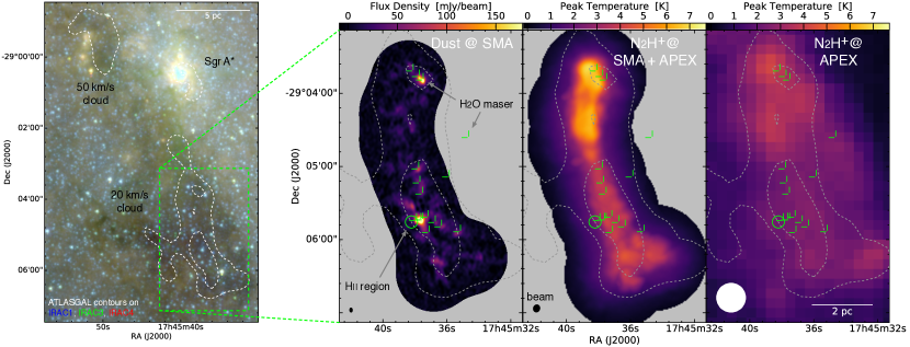
Figure 2: Example observations of the $\rm{}20\leavevmode\nobreak\ \rm{}km\,s^{-1}$ cloud. The left panel shows Spitzer IRAC data. The right panel presents dust continuum emission near $280\leavevmode\nobreak\ \rm{}GHz$ as observed by the SMA, combined APEX and SMA observations of the $\rm{}H_{2}H^{+}$ (3–2) transition, and APEX–only observations of the $\rm{}H_{2}H^{+}$ (3–2) transition covering a larger area. All panels are overlaid with contours of single–dish dust continuum emission at $870\leavevmode\nobreak\ \rm{}\mu{}m$ wavelength from APEX at arbitrary chosen levels. Note that we show SMA data not corrected for primary beam and missing extended emission to improve our visualization. The green circle indicates the location of an H ii region found by Ho et al. (1985), while green crosses give the location of water masers discovered by Lu et al. (2015).

We caution that the dust properties in the CMZ might differ from those prevalent in the solar neighborhood. For example, the relative Fe abundance in CMZ stars might exceed the solar neighborhood value by a factor $10^{0.11\pm 0.15}\approx{}1.3$ (Ryde & Schultheis, 2014). This suggests that the dust opacity might be larger by a similar factor. However, the metallicity of CMZ stars is highly diverse, including sub–solar values (Ryde & Schultheis, 2014; Do et al., 2015). In this situation we choose to adopt the aforementioned dust opacities that are representative for the solar neighborhood. A possible increase in dust opacities by a factor two would result in decreases of dust–derived masses by the same factor.

The interferometer maps are largely devoid of significant emission. This is a main feature of G0.253+0.016 that is already reported by Kauffmann et al. (2013b). The new observations now show that this relative absence of bright continuum emission is a general feature of CMZ molecular clouds. A more quantitative discussion of this trend is provided in Sec. 4.1.

We characterize the dust emission using dendrograms (Rosolowsky et al., 2008). In practice we run the ASTRODENDRO package on the intensity map resulting from the combination of SMA and APEX data. Intensities and flux densities are converted into column densities and masses as explained above. In essence this processing determines the mass and size for every closed contour in the continuum map (e.g., Fig. 1 of Kauffmann et al. 2010a). Here we refer to these structures as “fragments”, independent of their size. The fragment areas $A$ are converted into effective radii following $r_{\rm{}eff}=(A/\pi)^{1/2}$. We follow the emission down to the contour exceeding the noise level by a factor 3. Local maxima are assumed to be significant if the depth of the saddle point separating them from other local maxima exceeds the noise level by a factor 3. Only contours containing at least 10 pixels are considered, where pixels have a size of $0\aas@@fstack{\prime\prime}{}4$. We ignore unresolved structures, i.e., fragments with $r_{\rm{}eff}$ smaller than twice the beam radius. Such structures of small size form parts of larger fragments that are extracted in our search.

We complement this information on the clouds with information from the Herschel–based column density maps. Section 2.4 of Paper I describes how we determine the outer radius and total mass of every cloud, as well as the peak mass per beam of $37\arcsec$, corresponding to $r_{\rm{}eff}=0.74\leavevmode\nobreak\ \rm{}pc$. Table 1 of Paper I presents these measurements.

For reference we illustrate the conditions in Orion using a Herschel–based column density map of that region that is processed in the same way as the CMZ data. See Paper I for details. We use those data to characterize Orion on spatial scales $\gtrsim{}0.5\leavevmode\nobreak\ \rm{}pc$. The Bolocam data from Kauffmann et al. (2013b) are used to assess the mass reservoir on smaller spatial scales in this region. Dendrograms are used to characterize these maps. We adopt a dust temperature of 25 K for the analysis of the Bolocam maps of the Orion KL region on spatial scales $\lesssim{}0.1\leavevmode\nobreak\ \rm{}pc$ (Lombardi et al., 2014), consistent with temperatures of 25 to 30 K our maps show for dense gas immediately north of Orion KL.

Figure 3(a) presents the results from this analysis. The clouds have total integrated masses between $2.5\times{}10^{4}\,M_{\sun}$ and $3.4\times{}10^{5}\,M_{\sun}$ — when excluding Sgr D, for which no total mass could be determined due to insufficient contrast between cloud and background (see Paper I). These mass reservoirs are enclosed in radii of 1 to 7 pc. It is already obvious that on large spatial scale fragments within these clouds are very massive — and therefore dense — compared to fragments of similar size in Orion. A detailed discussion is presented in Secs. 3 and 4.

2.2 Characterization of $N_{2}H^{+}$ Line Emission

Here we briefly summarize procedures that are more completely described in Sec. 3.3 of Paper I. We think that the hyperfine structure of the $\rm{}N_{2}H^{+}$ (3–2) line is unlikely to have a significant impact on the observed line structure. A compact summary is, for example, provided by Table A1 of Caselli et al. (2002). This demonstrates that hyperfine satellites with velocity offsets exceeding $\pm{}0.6\leavevmode\nobreak\ \rm{}km\,s^{-1}$ only contain a few percent of the integrated relative intensities. Satellites within $\pm{}0.6\leavevmode\nobreak\ \rm{}km\,s^{-1}$ offset from the line reference frequency might broaden the observed lines by about $1\leavevmode\nobreak\ \rm{}km\,s^{-1}$, but the hyperfine structure is unlikely to have further impact on the observed spectra.

We characterize the cloud kinematics using several methods. First, we derive the velocity dispersion for the entire clouds. For this we average all single–dish APEX spectra available for a given cloud. The velocity dispersion is calculated as the second moment of these spectra and reported in Table 4 of Paper I. Second, we segment the emission in the maps combining single–dish and interferometer data on spatial scales $\sim{}1\leavevmode\nobreak\ \rm{}pc$ by drawing an iso–intensity surface in position–position–velocity ($p$–$p$–$v$) space at a threshold intensity corresponding to $1/3$ of the peak intensity of the respective map. Contiguous regions within these surfaces are considered to be coherent structures. We refer to these structures as “clumps”. The size of these clumps is characterized via the effective radius $r_{\rm{}eff}=(A/\pi)^{1/2}$, where $A$ is the area on the sky that contains all volume elements belonging to an extracted structure. Spectra integrated within the surfaces are used to obtain velocity dispersions. The latter property is only calculated if the peak intensity of a clump exceeds the threshold intensity for clump selection by a factor 2. Results are shown in Fig. 6 of Paper I. Third, we find all significant local maxima in $p$–$p$–$v$ space that are by a factor 5 above the noise, and that are separated from other significant maxima by troughs with a minimum depth $\geq{}1\leavevmode\nobreak\ \rm{}K$. This effectively selects structures at the spatial scale of the beam, i.e. $\sim{}0.1\leavevmode\nobreak\ \rm{}pc$. The spectra towards these locations are fit by multi–component Gaussian curves in order to obtain the velocity dispersions for the most narrow lines present in the clouds. This yields velocity dispersions of $0.6\leavevmode\nobreak\ {\rm{}to}\leavevmode\nobreak\ 2.2\leavevmode\nobreak\ \rm{}km\,s^{-1}$.

3 All CMZ Clouds have high Average Densities

All of the CMZ molecular clouds studied here have an unusually high average gas density. This is illustrated in Fig. 3 (top), where we compile data on gas reservoirs in the clouds as described in Sec. 2.1. As discussed in that section, the data are subject due to systematic uncertainties in assumptions about dust properties and other parameters. It is conceivable that all dust–based mass measurements are in error by factors $\sim{}2$, which would mean that all data are systematically shifted up or down from their true location. Relative errors between clouds or different spatial scales are less likely, though.

If we assume that the Orion A cloud and molecular clouds in the CMZ have similar 3D–geometries, then densities of CMZ clouds exceed those of Orion A by an order of magnitude at radii $\sim{}5\leavevmode\nobreak\ \rm{}pc$. For Sgr B2 the excess becomes a factor $\sim{}10^{2}$ at $5\leavevmode\nobreak\ \rm{}pc$ radius. This is remarkable, given that Orion A is one of the densest clouds in the wider solar neighborhood.

Note that this shows that the mass and density of the well–known cloud G0.253+0.016 is not exceptional in the CMZ. Instead we find that all major CMZ molecular clouds have very high masses and average densities when explored at radii well above a parsec.

Specifically, in Fig. 3 (top) we plot the mass and size of the target clouds from the analysis of Herschel maps explained in Sec. 2.1 on spatial scales $\geq{}0.7\leavevmode\nobreak\ \rm{}pc$. Specific numbers are taken from Table 1 of Paper I. On smaller spatial scales we use the dendrogram analysis of the combined SMA and APEX data. Here we first determine the smallest radius of a resolved fragment. Figure 3 (top) then shows the data for the most massive fragment that exceeds this smallest radius by at most 10%. The lines in Fig. 3 (top) effectively connect the mass–size measurement for the most massive “core” of $\sim{}0.1\leavevmode\nobreak\ \rm{}pc$ radius with the mass–size data of the $\sim{}1\leavevmode\nobreak\ \rm{}pc$ radius “clump” and the cloud in which the core is embedded.

On small spatial scales $\sim{}0.1\leavevmode\nobreak\ \rm{}pc$ we also include data for Sgr B2 extracted from a column density map presented by Schmiedeke et al. (2016). That study uses a range of continuum emission data sets obtained using LABOCA, the SMA, Herschel, and the VLA to obtain a three–dimensional model of the density distribution via radiative transfer modeling. This in particular takes the internal heating by star formation into account in a detailed fashion. Here we explore a map of the mass distribution as collapsed along the line of sight. The data point near 0.1 pc effective radius in Fig. 3 (top) is obtained by running a dendrogram analysis on that map in the same fashion as done for the SMA data presented in this paper.

For reference in Fig. 3 (top) we illustrate the conditions in Orion via the analysis of Herschel and Bolocam data explained in Sec. 2.1. We also indicate the mass–size threshold for high–mass SF from Kauffmann & Pillai (2010), $m(r)\geq{}870\,M_{\sun}\cdot{}(r/{\rm{}pc})^{1.33}$. Assuming a spherical geometry, uniform density, and a mean molecular weight per $\rm{}H_{2}$ molecule of 2.8 proton masses (Kauffmann et al., 2008), the mean $\rm{}H_{2}$ particle density is

$$n({\rm{}H_{2}})=3.5\times{}10^{4}\leavevmode\nobreak\ {\rm{}cm^{-3}}\cdot\left(\frac{M}{10^{4}\,M_{\sun}}\right)\cdot\left(\frac{r}{\rm{}pc}\right)^{-3}\,.$$ (2)

The Herschel–based masses and sizes on the largest scales of the CMZ clouds (Table 1 of Paper I) yield average densities in the range $(0.9\leavevmode\nobreak\ {\rm{}to}\leavevmode\nobreak\ 1.8)\times{}10^{4}\leavevmode\nobreak\ \rm{}cm^{-3}$. These densities are relatively high for Milky Way molecular clouds: Orion A, for example, has an average density of only $2.3\times{}10^{3}\leavevmode\nobreak\ \rm{}cm^{-3}$ for a radius of 4.4 pc.

For reference we also indicate the properties of the Arches cluster, one of the most massive stellar aggregates in the CMZ. Espinoza et al. (2009) find a mass of $2\times{}10^{4}\,M_{\sun}$ in an aperture of 0.4 pc radius. Note that Sgr B2 is the only CMZ region massive enough to form a cluster of this density structure by simply converting a fraction $<1$ of the mass residing at a fixed radius into stars. Walker et al. (2015) analyze this point in more detail. They conclude that it is indeed hard to form an Arches–like cluster in a single epoch of star formation. Walker et al. therefore suggest that massive clusters might form in a number of successive star formation events.

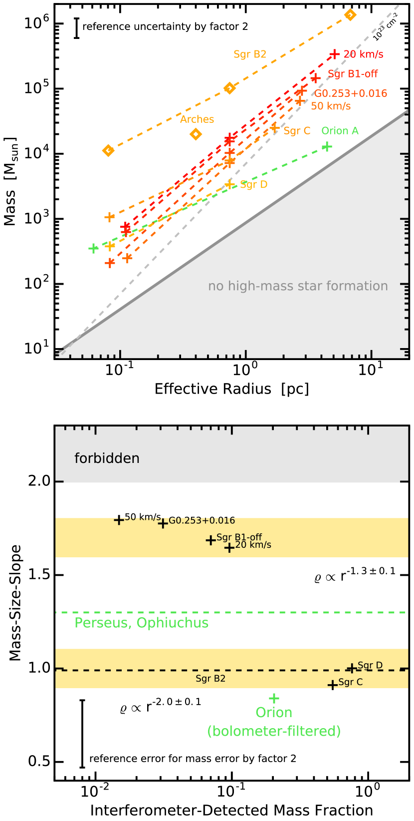
Figure 3: Analysis of the density structure of CMZ clouds. The top panel presents the mass–size data extracted for apertures of various sizes. See Sec. 2.1 for details. For reference, gray shading indicates the region of the parameter space where high–mass stars cannot form (Kauffmann & Pillai, 2010). The gray dashed line indicates a mean $\rm{}H_{2}$ column density of $10^{23}\leavevmode\nobreak\ \rm{}cm^{-2}$. The ordinate in the lower panel gives the mass–size slope ${\rm{}d}\,\ln(m)/{\rm{}d}\,\ln(r)$ measured in the upper panel on spatial scales $\lesssim{}1\leavevmode\nobreak\ \rm{}pc$, as explained in Sec. 4.1. The abscissa indicates the fraction of mass measured in the interferometer data which we consider to be the dense gas tracer. Horizontal lines are drawn for some regions for which only mass–size data are available (i.e., Perseus, Ophiuchus, and Sgr B2). Shaded regions highlight the parameter space occupied by spheres with indicated singular power–law density profiles. Green lines and markers present data from reference objects outside the CMZ. The gray shaded region contains solutions inconsistent with a fundamental assumption made in our analysis, i.e., that column densities decrease with increasing effective radius. Error bars in both panels indicate the change in properties in case the mass would change by a factor 2.

4 Dense Gas on Small Spatial Scales

4.1 Unusually Shallow Density Gradients in CMZ Clouds

One of the most puzzling aspects of CMZ clouds is that the embedded dense cores of about 0.1 pc radius have relatively low densities, compared to the high average densities inferred above (Fig. 3 [top]). The most massive cores in CMZ clouds studied here have masses similar to, and sometimes below, the one of the most massive core in Orion A, i.e., the Orion KL region. A representative mass of $400\,M_{\sun}$ within 0.1 pc radius gives a density of $1.3\times{}10^{6}\leavevmode\nobreak\ \rm{}cm^{-3}$. When compared to the average density on large spatial scales, the density in Orion A on 0.1 pc scale increases by a factor $\sim{}600$. In the CMZ clouds the density increase is lower by about an order of magnitude. This means that, compared to clouds like Orion, CMZ clouds have much more shallow density gradients. In Kauffmann et al. (2013b) we demonstrated this trend for G0.253+0.016. The new data show that this is a general trend for CMZ clouds.

The mass–size data in Fig. 3 (top) can be used to perform this analysis in more detail. We use the most massive features at 0.1 pc (interferometer data) and 0.7 pc radius (peak mass per Herschel beam) to measure mass–size slopes. These are defined as $b={\rm{}d}\,\ln(m)/{\rm{}d}\,\ln(r)$, which becomes $b\approx{}\ln(m[0.7\leavevmode\nobreak\ {\rm{}pc}]/m[0.1\leavevmode\nobreak\ {\rm{}pc}])/\ln(0.7\leavevmode\nobreak\ {\rm{}pc}/0.1\leavevmode\nobreak\ {\rm{}pc})$ in our situation. The resulting slopes are shown as the ordinate of Fig. 3 (bottom). For reference we also measure the mass–size slope using the data on Orion A shown in Fig. 3 (top). We further include slope measurements for the Perseus and Ophiuchus molecular clouds in the solar neighborhood ($d\leq{}300\leavevmode\nobreak\ \rm{}pc$) from Kauffmann et al. (2010b). These clouds only form low–mass stars. We find that, compared to other regions in the Milky Way, many CMZ clouds have unusually steep mass–size slopes.

These steep mass–size slopes imply unusually shallow density gradients. In Kauffmann et al. (2010b) we demonstrate that singular spherical power–law density profiles $\varrho{}\propto{}r^{-k}$ imply mass–size relations $m\propto{}r_{\rm{}eff}^{3-k}$ if $k\leq{}3$. A detailed analysis shows that these trends are generally preserved in a variety of density profiles, even if spherical symmetry does not apply. We can therefore use the relation $k\approx{}3-b$ to develop an idea of the density profiles found in CMZ clouds. Two such relations are indicated in Fig. 3 (bottom). We see that many CMZ molecular clouds have relatively shallow density profiles compared to other clouds in the Milky Way.

We find that Sgr B2, Sgr C, and Sgr D have a structure that is consistent with a density profile $\varrho{}\propto{}r^{-2}$, but that all other clouds have much more shallow density laws. This sets some CMZ clouds in a fascinating way apart from other Milky Way clouds, but this finding also means that there is a diversity in CMZ density gradients. Section 6 interprets these trends in the context of evolutionary differences among CMZ clouds.

We caution that there is a small chance that strong temperature gradients inside the clouds affect our measurements of $b$. As an example we consider the case that the temperature strongly decreases with decreasing $r$, so that the mass at $r=0.1\leavevmode\nobreak\ \rm{}pc$ is underestimated by a factor 2. In this case the true value of $b$ would be smaller by a moderate factor $\ln(2)/\ln(0.7\leavevmode\nobreak\ {\rm{}pc}/0.1\leavevmode\nobreak\ {\rm{}pc})\approx{}0.36$. The opposite would hold for temperatures increasing with decreasing $r$, i.e., true value of $b$ is larger than estimated here. Such trends could indeed in principle affect the data shown in Fig. 3 (bottom) and explain why the sample splits into populations with low and high $b$. Recall, however, that many CMZ dust emission peaks host star formation as evidenced by maser emission (e.g., Fig. 1 of Paper I). It seems unlikely that the true dust temperature drops significantly below the 20 K assumed here. In this case we would not expect that the true value of $b$ deviates significantly from the value reported in Fig. 3 (bottom). Also, since all CMZ clouds host some star formation, it is likely that all CMZ clouds are affected by similar errors in $b$. Temperature gradients alone are then not likely to explain why CMZ clouds differ in $b$.

4.2 Small Dense Gas Fractions in CMZ Clouds

The aforementioned mass–size analysis characterizes the density gradients of CMZ clouds. One other aspect of cloud structure is the fraction of mass concentrated in the most massive and compact features. This dense gas fraction is characterized here. We find this property to be unusually small in many CMZ clouds.

We stress that here we can only present approximate measures of the dense gas fraction. The problem is that there are no clear–cut definitions of total cloud mass and the mass of high–density gas. For example, here we adopt the working definition that gas all material detected by the interferometer resides in dense structures. This is not necessarily true, and it is well possible that a low–density filament or sheet seen edge–on will be just as detectable as denser spherical cloud fragment. Here we derive a ratio between integrated intensities instead of masses. The mass of dense gas is characterized by integrating the flux in the interferometer–only SMA images that are not corrected for the primary beam pattern. In this calculation we only include emission exceeding the noise in the images by a factor 2. We need to obtain a measure of the total cloud mass that relates to the area imaged by the interferometer. Our measure is based on the aforementioned ATLASGAL data (Schuller et al., 2009) that are scaled to the observing frequency of the SMA (see Appendix A.1 of Paper I). Towards every CMZ cloud we first multiply the ATLASGAL data with the sensitivity pattern of the SMA interferometer observations. We then integrate the scaled intensities to obtain a measure of the total cloud mass. The dense gas fraction is then approximated by dividing the interferometer–only flux density by the one derived from the scaled ATLASGAL images. This ratio would be 1 if the compact structures picked up by the SMA contained all the flux seen in the ATLASGAL maps. This ratio is shown on the abscissa of Fig. 3 (bottom). We obtain a reference value for the Orion A molecular cloud using our Bolocam map: the bolometer observations of a cloud at about 420 pc distance very roughly approximate the spatial filtering induced by the interferometer at 8.3 kpc distance. We stress that a more detailed analysis is highly desirable but not straightforward. Specifically we divide the mass obtained from our Bolocam map (assuming a temperature of 15 K) by the Herschel–based total mass in Fig. 3 (top).

Figure 3 (bottom) demonstrates that the dense gas fraction varies within the CMZ, but that most CMZ clouds have dense gas fractions that are by factors of 2 to 10 below the reference value estimated for Orion A. Similar conclusions were reached by Johnston et al. (2014) and Rathborne et al. (2014), who studied probability density functions (PDFs) of the cloud column density: some CMZ molecular clouds are relatively free of dense gas that could form stars. Interestingly, the Sgr C and Sgr D clouds, that stand out with mass–size slopes unusually flat for CMZ clouds, also stand out in relatively high dense gas fractions. We return to this point in Sec. 6 on evolutionary differences between CMZ clouds.

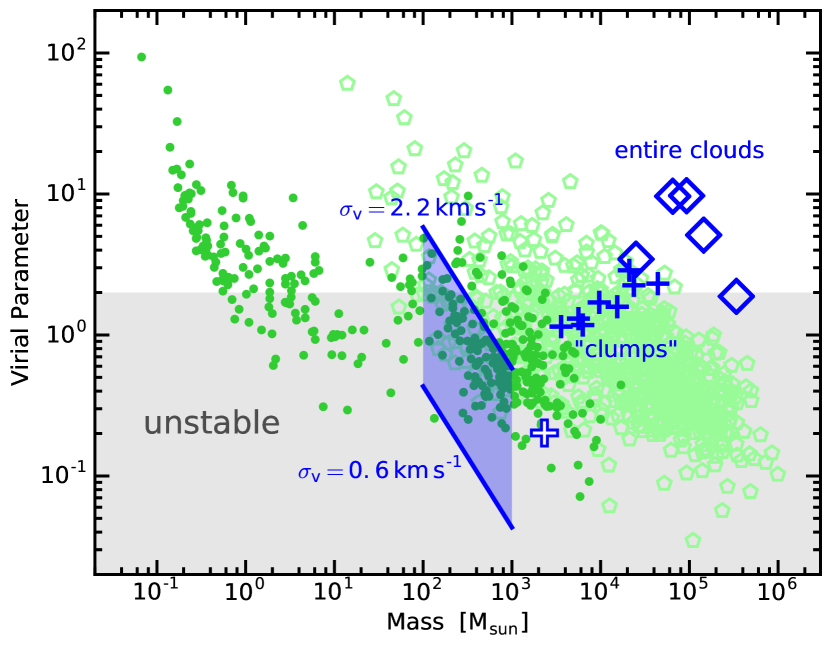
Figure 4: Summary of the virial parameter measurements $\alpha$ from Sec. 5. Blue symbols give data for structures of varying spatial size explored in this paper. See Sec. 2.2 for terminology and details. The blue cross with white filling indicates data for the Sgr D region that probably resides outside the CMZ as studied here. Dark green bullets indicate the properties of reference Milky Way clouds that were explored in emission lines of $\rm{}N_{2}H^{+}$ and $\rm{}NH_{3}$ tracing dense gas. Values for these are taken from the Kauffmann et al. (2013a) compilation. Light green diamonds give CO–based data for the lower density gas in Milky Way clouds reported in the same compilation. The blue shaded area gives the virial parameter that would hold for cloud fragments of radius 0.1 pc that have masses and velocity dispersions within the ranges indicated in the figure. Gray shading shows where $\alpha<\alpha_{\rm{}cr}\approx{}2$, indicating the domain where non–magnetized hydrostatic equilibria become unstable to collapse.

5 Gravitational Binding

In Kauffmann et al. (2013b) we reasoned that the cloud G0.253+0.016 is only marginally gravitationally bound on large spatial scales, but that some of the embedded substructures might well be bound and unstable to collapse. Here we confirm this finding and establish it as a general trend for CMZ clouds (e.g., Fig. 4).

The combined information on gas densities and kinematics allows to calculate the virial parameter, $\alpha=5\,\sigma^{2}(v)\,R/(G\,M)$, as defined by Bertoldi & McKee (1992). Measures of mass and velocity dispersion refer to a given aperture of radius $R$. Clouds are unstable to collapse if $\alpha<\alpha_{\rm{}cr}$. The critical value depends on the nature of the pressure supporting the cloud, with values $\alpha_{\rm{}cr}\approx{}2$ being appropriate in most cases where magnetic fields are absent (Kauffmann et al., 2013a).

We caution that the concept of the virial parameter ignores several processes that might be relevant in the CMZ. For example, the gravitational potential of the CMZ can subject clouds to shear. The fast internal motions of some clouds might already reflect this shear, while in other clouds shear might just be about to set in and has not yet increased internal motions. These shear motions will stabilize clouds against collapse, and (depending on whether shear has set in or not) the observed virial parameter might thus underestimate a cloud’s ability to resist self–gravity. But CMZ clouds can also be subject to compressive tides (Sec. 1) that increase self gravity. From this perspective the virial parameter might overestimate how well a cloud can withstand collapse. The impact of shear and tides should be most significant on the largest spatial scales. This suggests that virial parameter assessments on entire clouds must be treaded with caution, while data on smaller structures can be interpreted more reliably.

Figure 4 presents a virial analysis that uses the information on cloud kinematics from Paper I (see Sec. 2.2). Given the range of velocity dispersions (Fig. 7 of Paper I) and mass reservoirs (Fig. 3 [top]) on small spatial scales, we adopt ranges for velocity dispersions and masses instead of fixed numbers. A radius of 0.1 pc is assumed for the smallest structures, corresponding to the spatial scale on which the smallest interferometer–detected structures are extracted in Fig. 3 (top). Note that no direct mass measurements are available for the “clumps” of about 1 pc radius: here we adopt a mean $\rm{}H_{2}$ column density of $2\times{}10^{23}\leavevmode\nobreak\ \rm{}cm^{-2}$ to calculate a mass on the basis of the measured radii. This is a plausible value, as can be gleaned from Fig. 3 (top). In this respect the properties for the “clumps” in Fig. 4 should be taken as an estimate instead of a real measurement. Walker et al. (2015) obtain slightly lower virial parameters for some of our clouds. Their results resemble those we obtain for the “clumps” of intermediate size. It is plausible that this is a consequence of their scheme to reject unrelated velocity components. The method Walker et al. use to measure velocity dispersions resembles the one we use for our “clumps”.

It appears that the clouds on largest spatial scales are unbound or only marginally bound. It is thus possible that several of these clouds will disperse in the future. The situation is markedly different for the “clumps” with radii of order 1 pc. It seems plausible or even likely that many of these structures will remain bound. These are excellent conditions for current or future star formation. The densest interferometer–detected cores are very likely subject to signifiant gravitational binding, depending on how exactly gas motions and density structure combine. Rathborne et al. (2015) and Lu et al. (2015) obtain similar results for G0.253+0.016 and the $20\leavevmode\nobreak\ \rm{}km\,s^{-1}$ cloud, respectively.

In summary the data presented here suggest that the conditions are conducive for star formation on small spatial scales, but that it is not clear that the entire clouds will participate in this process. Note, however, that this analysis ignores magnetic fields (as well as tidal forces and shear). Pillai et al. (2015) show that, at least in G0.253+0.016, magnetic forces due to a field $\sim{}5.4\leavevmode\nobreak\ \rm{}mG$ are an important and possibly dominating factor in the total energy budget. This might also hold for other CMZ clouds. Magnetic fields have the effect of reducing the critical virial parameter (Kauffmann et al., 2013a). Provided magnetic fields have a sufficient strength, this might mean that the physical conditions in CMZ clouds are not favorable for star formation.

6 Discussion: Suppressing CMZ Star Formation

We return to the problem illustrated in Fig. 1, i.e., the question why CMZ star formation in dense gas is suppressed by a factor $\gtrsim{}10$ compared to other regions in the Milky Way. Here we collect some of the factors examined above and interpret them in context.

6.1 Moderate CMZ Star Formation Density Thresholds

The most straightforward explanation of suppressed CMZ star formation would be the existence of a high density threshold for star formation that is not overcome by CMZ clouds. Kruijssen et al. (2014) explore this option on the basis of the observations by Longmore et al. (2013a). They conclude that an SF threshold $\rm{}H_{2}$ particle density $\gtrsim{}10^{7}\leavevmode\nobreak\ \rm{}cm^{-3}$ is needed to explain the observed level of SF suppression, provided steep power–law probability density functions (PDFs) of gas density prevail in clouds. Log–normal distributions, which are more commonly observed in molecular clouds (e.g., Kainulainen et al. 2009), imply threshold densities $\gtrsim{}3\times{}10^{8}\leavevmode\nobreak\ \rm{}cm^{-3}$. Kruijssen et al. also argue that the fast supersonic motions in CMZ clouds would in fact imply threshold densities $\approx{}3\times{}10^{7}\leavevmode\nobreak\ \rm{}cm^{-3}$, based on single–dish observations of clouds. Here we re–examine this latter claim based on our independent measurements of gas density and line width. In particular, we include the observations of low velocity dispersions in our interferometer maps.

Kruijssen et al. (2014) build their analysis on previous work by Krumholz & McKee (2005) and Padoan & Nordlund (2011). These authors argue that the threshold $\rm{}H_{2}$ particle density for star formation in a cloud of one–dimensional Mach number $\mathcal{M}$ exceeds the mean cloud density by a factor

$$\frac{n_{\rm{}SF,lim}}{\langle{}n\rangle}=(1.2\pm{}0.4)\cdot\alpha\,\mathcal{M}^{2}\,,$$ (3)

where $\alpha$ is the virial parameter. The range in the proportionality constant reflects the differences between the theoretical derivations by different groups. We adopt an approximate value of 1.2 in the following. Kruijssen et al. (2014) use average properties of CMZ clouds gleaned from single–dish data to evaluate this relation. They adopt Mach numbers of order 30, average densities of a few $10^{4}\leavevmode\nobreak\ \rm{}cm^{-3}$, and virial parameters of order 1. This yields the aforementioned values $n_{\rm{}SF,lim}\approx{}3\times{}10^{7}\leavevmode\nobreak\ \rm{}cm^{-3}$. The GCMS provides more single–dish data on clouds and expands the relevant observational picture because the interferometer observations reveal rather narrow lines of $0.6\leavevmode\nobreak\ {\rm{}to}\leavevmode\nobreak\ 2.2\leavevmode\nobreak\ \rm{}km\,s^{-1}$ on spatial scales $\sim{}0.1\leavevmode\nobreak\ \rm{}pc$.

First consider entire clouds. In Paper I we show that $\mathcal{M}=\sigma(v)/\sigma_{{\rm{}th},\langle{}m\rangle{}}(v)$ is between 15 and 40 for our target clouds on spatial scales probed by single–dish data, where $\sigma_{{\rm{}th},\langle{}m\rangle{}}(v)$ is the thermal velocity dispersion (here evaluated at 50 K) at the mass of the mean free particle, $\langle{}m\rangle{}=2.33\,m_{\rm{}H}$ (see Paper I). We substitute the specific observed values of $\alpha$ and $\mathcal{M}$ for our target clouds in Eq. (3). This gives $n_{\rm{}SF,lim}=(0.1\leavevmode\nobreak\ {\rm{}to}\leavevmode\nobreak\ 2)\times{}10^{8}\leavevmode\nobreak\ \rm{}cm^{-3}$. These numbers are broadly consistent with the results by Kruijssen et al. (2014).

Alternatively we can use Eq. (3) to evaluate the SF threshold density for structures of size $\sim{}0.1\leavevmode\nobreak\ \rm{}pc$. This is particularly interesting because Paper I derives much lower velocity dispersions and Mach numbers for these structures. To do this evaluation we substitute the definitions of the thermal velocity dispersion (Eq. 1 from Paper I) and the virial parameter in Eq. (3). We obtain

$$\frac{n_{\rm{}SF,lim}}{\langle{}n\rangle}\approx 8.1\,\left(\frac{\sigma(v)}{\rm{}km\,s^{-1}}\right)^{4}\,\left(\frac{T_{\rm{}gas}}{50\leavevmode\nobreak\ \rm{}K}\right)^{-1}\,\left(\frac{R}{0.1\leavevmode\nobreak\ \rm{}pc}\right)\,\left(\frac{M}{100\,M_{\sun}}\right)^{-1}\,,$$ (4)

where $T_{\rm{}gas}$ is the gas temperature. We pick a representative mass of $400\,M_{\sun}$ for the mass of structures of 0.1 pc radius. Figure 3 (top) shows that the actual masses differ by a factor only $\sim{}2$ from this, if we exclude the much more massive structures in Sgr B2. Given the uncertainty in velocity dispersions on this spatial scale, we vary $\sigma(v)$ between 0.6 and $2.2\leavevmode\nobreak\ \rm{}km\,s^{-1}$. For these parameters we find that $n_{\rm{}SF,lim}/\langle{}n\rangle\approx{}0.3\leavevmode\nobreak\ {\rm{}to}\leavevmode\nobreak\ 47$. A mean density $\langle{}n\rangle=1.4\times{}10^{6}\leavevmode\nobreak\ \rm{}cm^{-3}$ holds for 0.1 pc radius and $400\,M_{\sun}$ mass (Eq. 2). This implies values of $n_{\rm{}SF,lim}$ between $4\times{}10^{5}\leavevmode\nobreak\ \rm{}cm^{-3}$ and $7\times{}10^{7}\leavevmode\nobreak\ \rm{}cm^{-3}$. A representative velocity dispersion is arguably given by the median value of the smallest velocity dispersions found in the clouds, $\min(\sigma_{\rm{}int}[v])$ (Table 5 of Paper I). This median value is $1.1\leavevmode\nobreak\ \rm{}km\,s^{-1}$. Choosing this velocity dispersion gives $n_{\rm{}SF,lim}/\langle{}n\rangle=3$ and thus $n_{\rm{}SF,lim}=4\times{}10^{6}\leavevmode\nobreak\ \rm{}cm^{-3}$. This latter result is at the lower limit of the range in SF threshold densities considered by Kruijssen et al. (2014).

Note, however, that none of these considerations take the role of the magnetic field into account. Section 6.3 discusses that this field might play a major role in shaping clouds.

In summary we generally derive SF threshold densities consistent with what Kruijssen et al. (2014) estimate via Eq. (3) from single–dish data. The interferometer data may, however, hint at SF threshold densities that are as low as $10^{6}\leavevmode\nobreak\ \rm{}cm^{-3}$, which is well below densities $10^{7}\leavevmode\nobreak\ \rm{}cm^{-3}$ deemed plausible before. Given our results, it appears plausible to adopt $n_{\rm{}SF,lim}=10^{7\leavevmode\nobreak\ {\rm{}to}\leavevmode\nobreak\ 8}\leavevmode\nobreak\ \rm{}cm^{-3}$ for the CMZ. Kruijssen et al. (2014) estimate that $n_{\rm{}SF,lim}\approx{}10^{4}\leavevmode\nobreak\ \rm{}cm^{-3}$ in the solar neighborhood. The values for the CMZ are thus much higher, and this difference might — relative to the solar neighborhood — help to suppress CMZ star formation as observed. However, the estimated values of $n_{\rm{}SF,lim}=10^{7\leavevmode\nobreak\ {\rm{}to}\leavevmode\nobreak\ 8}\leavevmode\nobreak\ \rm{}cm^{-3}$ are at the lower limit of the threshold densities between $10^{7}\leavevmode\nobreak\ \rm{}cm^{-3}$ and $\gtrsim{}3\times{}10^{8}\leavevmode\nobreak\ \rm{}cm^{-3}$ Kruijssen et al. (2014) require to suppress CMZ star formation at the observed level. For example, rather steep power–law PDFs need to prevail to bring the predicted threshold densities from Eq. (3) in agreement with the thresholds Kruijssen et al. estimate from the observed SF. This suggests to look for additional factors that might suppress CMZ star formation.

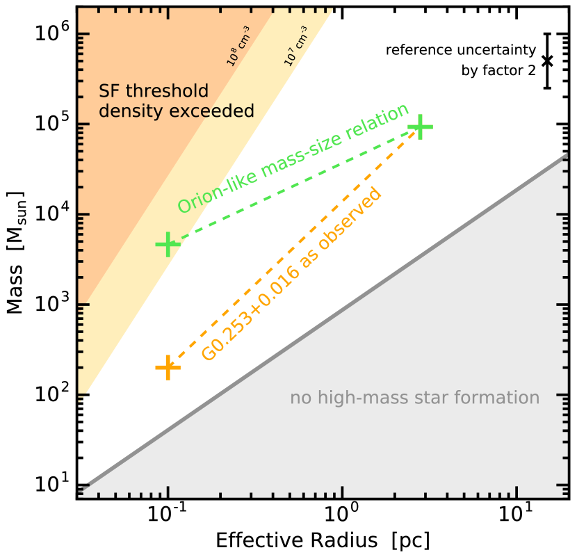
Figure 5: The impact of mass–size slopes — i.e., density gradients — on CMZ star formation. The gray shading is taken from Fig. 3. The brown–orange shading indicates where spheres would exceed the star formation density threshold. The shading gradient indicates the uncertainty in $n_{\rm{}SF,lim}$, here taken to be in the range $10^{7\leavevmode\nobreak\ {\rm{}to}\leavevmode\nobreak\ 8}\leavevmode\nobreak\ \rm{}cm^{-3}$. The orange cross and dashed line indicates the mass–size trend observed for G0.253+0.016. The green crosses and dashed line gives the mass–size relation of a model cloud that has the same total mass and size as G0.253+0.016, but follows a more shallow mass–size relation (i.e., steeper density gradient), here taken from observations of Orion. The error bar indicates the a representative uncertainty in mass measurements by a factor 2 (Sec. 3). In summary this diagram shows that shallow CMZ density laws help to suppress star formation because little or no gas at all exceeds $n_{\rm{}SF,lim}$.

6.2 Suppressed SF from Shallow Density Gradients

It appears that the cloud density structure plays a key role in determining the star formation rate of the CMZ clouds. Specifically, it emerges that the shallow density gradients — and corresponding steep mass–size relations — found in Sec. 4.1 are essential to understand CMZ star formation. This is illustrated in Fig. 5.

Section 6.1 yields SF threshold densities $n_{\rm{}SF,lim}=10^{7\leavevmode\nobreak\ {\rm{}to}\leavevmode\nobreak\ 8}\leavevmode\nobreak\ \rm{}cm^{-3}$. This range is indicated in Fig. 5. Now consider G0.253+0.016 as an example. The observed mass–size trend indicated in Fig. 5 steers clear of the domain where the SF threshold density would be exceeded. For comparison Fig. 5 also shows the mass–size trend G0.253+0.016 would have if it had the same mass–size slope as Orion A (that value is taken from Fig. 3). Here we see that the density in G0.253+0.016 would then actually reach values close to the SF density threshold. Similar trends hold for all other CMZ clouds explored here. This excludes the notable exception of Sgr B2, which reaches densities well in excess of the thresholds considered here.

For this reason we argue that the low star formation activity of CMZ clouds is chiefly a consequence of the unusually shallow density gradients of CMZ clouds. Theoretical research into CMZ cloud structure must begin to explore this critical trend.

We speculate that shallow density gradients can emerge when the clouds are not tightly bound by self–gravity. In that case gravitational forces cannot help in concentrating mass into compact structures. This has the consequence that cloud fragments much smaller than the total cloud size will only contain a relatively small fraction of the total cloud mass. In other words: such a region has a relatively steep mass–size relation, implying shallow density gradients. Figure 4 shows indeed that CMZ clouds are at best marginally bound by self–gravity. This supports the picture outlined above. Further, in Sec. 1 we describe that CMZ clouds are subject to compressive tides and are further confined by significant thermal pressure that forces any gas at moderate temperatures $\lesssim{}100\leavevmode\nobreak\ \rm{}K$ to reside at densities $\gtrsim{}10^{4}\leavevmode\nobreak\ \rm{}cm^{-3}$. These two mechanisms might help to produce massive clouds of high average density that are unbound.

6.3 Suppressed SF from Strong Magnetic Fields

The strong magnetic field penetrating CMZ clouds might be another important factor in the suppression of CMZ star formation. The gas is pervaded by a strong magnetic field of a few $10^{3}\leavevmode\nobreak\ \rm{}\mu{}G$ (Yusef-Zadeh et al., 1984; Uchida et al., 1985; Chuss et al., 2003; Novak et al., 2003). This field also penetrates individual CMZ clouds with a strength that is high enough to prevent the global collapse of clouds (Pillai et al., 2015). It is conceivable that the shallow density profiles described above are a direct consequence of magnetic fields dominating over self–gravity as well as turbulence.

The observational properties of the CMZ magnetic field are well established at this point (see, e.g., Morris 2014 for a review). What is less clear is the origin of this strong field, and how exactly it couples to the orbit on which clouds travel around in the CMZ. This makes it hard to gauge the exact role the magnetic field might play for the evolution of CMZ molecular clouds.

6.4 A Note of Caution: Disconnects between SF and Density Structure

We note that the current cloud structure can have little relation to the recent star formation activity. Consider the $50\leavevmode\nobreak\ \rm{}\,km\,s^{-1}$ cloud. As evident from the dust continuum emission maps in Paper I, and quantified by the mass–size data in Fig. 3, this cloud is devoid of evidence for dense and massive clumps that are definitely needed to form high–mass stars. At the same time the cloud hosts four H ii regions with ages of about 1 Myr or less (Table 5 and Appendix C of Paper I). This finding suggests that the cloud density structure has evolved significantly since it gave birth to the high–mass stars powering the H ii regions. This is plausible: cloud structure can evolve on a time scale similar to the flow crossing times $\sim{}3\times{}10^{5}\leavevmode\nobreak\ \rm{}yr$ obtained in Sec. 3.4 of Paper I, which is shorter than the aforementioned lifetimes of H ii regions.

In other CMZ clouds we find a more direct connection between the young stars and dense cloud fragments. For example, Lu et al. (2015) study the $20\leavevmode\nobreak\ \rm{}km\,s^{-1}$ cloud and detect a population of water masers closely associated with dense structures seen in SMA maps of dust emission.

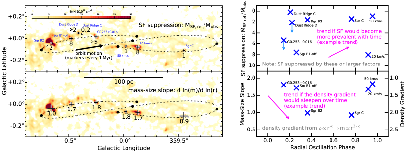
Figure 6: The spatial distribution of cloud properties. Blue labels in the top map give cloud names. Symbol sizes and labels in the top map indicate the factor by which the star formation activity in the dense gas is suppressed relative to a typical Milky Way reference value provided by Eq. (5). Symbol sizes and labels in the bottom map give the mass–size slope derived from the cloud structure data on spatial scales $\lesssim{}1\leavevmode\nobreak\ \rm{}pc$. A dotted line in the maps shows part of the orbit for CMZ clouds proposed by Kruijssen et al. (2015). The background maps present a column density map derived from Herschel dust emission data, as derived in this paper. The panels on the right present the same information on SF suppression and mass–size slopes as a function of the radial phase of the orbit proposed by Kruijssen et al. (2015). The magenta arrows indicate very roughly how a property might change, e.g., if SF suppression would decrease over time or in case density gradients would steepen over time: the directions of arrows matter (i.e., up or down vs. phase), but their position or placement does not. In summary the observed trends suggests that clouds do not follow a systematic evolutionary pattern as they orbit the CMZ.

6.5 No systematic Cloud Evolution along CMZ Orbit

Figure 6 presents the mass–size slopes and star formation rates in the context of the orbit of CMZ clouds inferred by Kruijssen et al. (2015). Longmore et al. (2013b) suggest that clouds evolve as they move along the orbit. In particular the latter group proposes a sequence in which dense clouds form (or get strongly compacted) near the location of G0.253+0.016 via compression induced by the gravity of the CMZ potential centered on the $\rm{}Sgr\leavevmode\nobreak\ A^{\ast}$ region, start to evolve towards star formation, and become efficient star–forming clouds as they move along the orbit towards Sgr B2. In other words, the pericenter passage sets an absolute time marker in these models of cloud evolution. Here we cannot evaluate whether the pericenter passage affects the structure of the clouds. However, our data only provide mixed evidence for scenarios in which the pericenter passage induces a systematic evolution towards SF with increasing orbital phase (measured with respect to the pericenter location).

Figure 6 places our data into the overall orbital context of the CMZ. We use Fig. 6 (left) to present the data in the context of a map, while Fig. 6 (right) shows the same information but against the orbital phase. Specifically we consider the orbital oscillations in radius, that have a period of $2.03_{-0.18}^{+0.70}\leavevmode\nobreak\ \rm{}Myr$ (Kruijssen et al. 2015; the other periods are $3.69_{-0.30}^{+0.68}\leavevmode\nobreak\ \rm{}Myr$ in azimuth and $2.27_{-0.34}^{+0.70}\leavevmode\nobreak\ \rm{}Myr$ perpendicular to the Galactic Plane, respectively). The radial orbital phase is measured with respect to the pericenter passage. The time since pericenter passage is taken from Table 2 of Kruijssen et al. (2015).

Figure 6 (top) summarizes the ratio $\dot{M}_{\rm{}SF,ref}/\dot{M}_{\rm{}obs}$ between the observed star formation rate, $\dot{M}_{\rm{}obs}$, and the reference value taken from Lada et al. (2010),

$$\dot{M}_{\rm{}SF,ref}=(4.6\pm{}2.6)\times{}10^{-8}\,M_{\sun}\,{\rm{}yr}^{-1}\cdot{}(M_{\rm{}dense}/M_{\odot})\,.$$ (5)

Lada et al. take $M_{\rm{}dense}$ to be the cloud mass residing at a column density corresponding to a visual extinction $A_{V}\gtrsim{}7\leavevmode\nobreak\ \rm{}mag$. The ratio $\dot{M}_{\rm{}SF,ref}/\dot{M}_{\rm{}obs}$ indicates the factor by which star formation in a region is suppressed. Here we use the total cloud masses from Table 1 in Paper I, representing masses at $A_{V}\gtrsim{}100\leavevmode\nobreak\ \rm{}mag$, to evaluate Eq. (5). The star formation rates are taken from Table 7 in Paper I. These latter estimates are largely based on the number of radio–detected H ii regions that are embedded in a cloud.

We do find an increase in the dense gas star formation efficiency between G0.253+0.016 and Sgr B2 by a factor $\gtrsim{}3$. However, current data do not indicate a monotonic increase of the star formation activity, as indicated by the case of the Dust Ridge C cloud where $\dot{M}_{\rm{}obs}$ is up to $5\,\dot{M}_{\rm{}SF,ref}$ and the case of significantly suppressed star formation in the Sgr B1–off region between Sgr B2 and Dust Ridge C.

The situation is even less clear — though not necessarily in conflict with the Longmore et al. (2013b) model — when considering star formation in the $20\leavevmode\nobreak\ \rm{}km\,s^{-1}$ and $50\leavevmode\nobreak\ \rm{}km\,s^{-1}$ clouds. First, the locations of these clouds along the proposed orbit are separated by only about $10^{5}\leavevmode\nobreak\ \rm{}yr$, while their SF rate per unit dense gas varies sharply by a factor $\sim{}9$. It is difficult to imagine how this difference in SF rate should emerge over such a small time scale. Second, the $50\leavevmode\nobreak\ \rm{}km\,s^{-1}$ cloud show significant star formation ahead of the pericenter passage. That said, Longmore et al. (2013b) only speculate that their model holds for clouds between G0.253+0.016 and Sgr B2, and Kruijssen et al. (2015) show that the $20\leavevmode\nobreak\ \rm{}km\,s^{-1}$ and $50\leavevmode\nobreak\ \rm{}km\,s^{-1}$ clouds are disconnected from the aforementioned sequence of clouds. Still, the $20\leavevmode\nobreak\ \rm{}km\,s^{-1}$ and $50\leavevmode\nobreak\ \rm{}km\,s^{-1}$ clouds highlight that the cloud state before pericenter passage will influence the subsequent cloud evolution.

Figure 6 (bottom) presents measures of the gas density distribution, i.e., the mass–size slope. We do find noteworthy variations within the CMZ: Sgr B2 and Sgr C have slopes significantly different from all other clouds along the proposed orbit studied here. However, there is only weak evidence for any systematic trend. In particular we see no change between G0.253+0.016 and Sgr B1–off: such a trend would probably be expected if clouds were evolving towards star formation between G0.253+0.016 and Sgr B2. That said, the Sgr B2 region has the shallow mass–size slopes naively expected for regions that evolve towards star formation by increasing their density gradients. Still, if the difference between Sgr B1–off and Sgr B2 is a result of evolution, then this process must be completed in the about $3\times{}10^{5}\leavevmode\nobreak\ \rm{}yr$ that it takes to travel between the clouds along the orbit. This would be an exceptionally fast evolution in cloud structure, comparable to the dynamic crossing times for CMZ clouds (Sec. 3.4 of Paper I).

Note that the inverse trend is observed for the evolution between Sgr C and the $50\leavevmode\nobreak\ \rm{}km\,s^{-1}$ cloud, i.e., the mass–size slope increases along the orbit. This is clearly not expected for straightforward evolution towards star formation. Some additional hypotheses are required to explain this trend.

We stress that some of this discussion depends on whether all CMZ clouds do indeed follow the orbit proposed by Kruijssen et al. (2015). Their model provides a good mathematical description of the structure of the CMZ. Note, however, that some studies find evidence for interaction of the $20\leavevmode\nobreak\ \rm{}km\,s^{-1}$ and $50\leavevmode\nobreak\ \rm{}km\,s^{-1}$ with the inner Galactic Center environment. See Herrnstein & Ho (2005) for a discussion of the evidence, including material taken from earlier sources. Such interactions would place these two clouds within about 10 pc from $\rm{}Sgr\leavevmode\nobreak\ A^{\ast}$. This would be inconsistent with the Kruijssen et al. orbital model, and such deviant clouds should not be placed in Fig. 6 (right).

This leaves us with a mixed record on evidence for an evolutionary sequence along the Kruijssen et al. (2015) orbit that is primarily controlled by the orbital phase — i.e., the separation in space or time from the closest pericenter passage along the CMZ orbit. The spatial distribution of CMZ star formation does not support this idea, while there is limited evidence from the analysis of cloud density structure.

We stress that these observations complement the ideas forwarded by Longmore et al. (2013b) and Kruijssen et al. (2015). First, as noted before, we cannot test whether a given cloud is modified during pericenter passage, as proposed by Longmore et al. (2013b). Second, we only explore whether the orbital phase is the primary parameter controlling SF. It is well possible that factors like initial density, etc., also play a role and that clouds do follow an evolutionary sequence as they orbit the CMZ — but on an individual time line that is not necessarily similar to the one of neighboring CMZ clouds. A need to include properties of individual clouds would reduce the potential value of an absolute time line (i.e., with respect to the pericenter passage) and make model tests very complex. In this sense our observations point towards the idea of Kruijssen et al. (2015; their Sec. 4.2) that the evolution along the orbit is — if at all present — to be seen in a statistical sense: there can be variation between clouds at given orbital phase, depending on initial conditions. More measurements than accessible here are needed to explore this statistical view.

7 Summary

We present the first comprehensive study of the density structure of several molecular clouds in the Central Molecular Zone (CMZ) of the Milky Way. This is made possible by using data from the Galactic Center Molecular Cloud Survey (GCMS), the first systematic study resolving all major molecular clouds in the CMZ at interferometer angular resolution (Kauffmann et al. 2016; hereafter Paper I).

We combine the new characterization of GCMS dust emission data with information on the cloud kinematics and the star formation (SF) activity from Paper I. This leads us to a number of conclusions.

• All major CMZ molecular clouds have high average densities $\sim{}10^{4}\leavevmode\nobreak\ \rm{}cm^{-3}$ when explored on spatial scales $\gtrsim{}1\leavevmode\nobreak\ \rm{}pc$ (Sec. 3). This is illustrated in Fig. 3 (top). The well–known cloud G0.253+0.016 (a.k.a. the “Brick”) is one of several massive and dense clouds in the CMZ.

• Many CMZ molecular clouds have unusually shallow density gradients (Sec. 4.1). This is reflected in mass–size slopes that are much steeper than what is found in, e.g., SF regions in the solar neighborhood (Fig. 3). For example, the structure of many CMZ clouds is consistent with — highly simplistic — power–law density profiles resembling $\varrho{}\propto{}r^{-1.3}$ (Fig. 3 [bottom]). In addition, a relatively small fraction of the cloud mass is concentrated in such dense structures (Sec. 4.2, Fig. 3 [bottom]).

• Random “turbulent” gas motions imply an SF density threshold in the range $10^{7\leavevmode\nobreak\ {\rm{}to}\leavevmode\nobreak\ 8}\leavevmode\nobreak\ \rm{}cm^{-3}$ (Sec. 6.1). These high densities probably help to suppress SF in the CMZ. A further critical factor for SF suppression appear to be the unusually shallow density gradients observed in many CMZ clouds. The resulting steep mass–size laws imply that very little mass in the clouds will exceed the SF density threshold (Sec. 6.2, Fig. 5). We speculate that these shallow density laws are a consequence of weak gravitational binding of the clouds.

• We find mixed evidence that clouds systematically evolve towards SF with increasing orbital phase along the CMZ orbit (i.e., with respect to pericenter passage; Sec. 6.5). These observations can help to refine ideas about CMZ cloud evolution forwarded by Longmore et al. (2013b) and Kruijssen et al. (2015). Specifically, we find no clear trend in star formation activity per unit dense gas (Fig. 6 [top]), while we do find a trend in density gradients (i.e., mass–size slopes; Fig. 6 [bottom]). However, the interpretation of this latter trend as a consequence of cloud evolution along the orbit requires massive changes of cloud structure on time scales of order 0.3 Myr, which we consider to be questionable.