The decay $\eta\to 3\pi$: study of the Dalitz plot and extraction of the quark mass ratio $Q$

Abstract

The $\eta\to 3\pi$ amplitude is sensitive to the quark mass difference $m_{u}-m_{d}$ and offers a unique way to determine the quark mass ratio $Q^{2}\equiv(m_{s}^{2}-m_{ud}^{2})/(m_{d}^{2}-m_{u}^{2})$ from experiment. We calculate the amplitude dispersively and fit the KLOE data on the charged mode, varying the subtraction constants in the range allowed by chiral perturbation theory. The parameter-free predictions obtained for the neutral Dalitz plot and the neutral-to-charged branching ratio are in excellent agreement with experiment. Our representation of the transition amplitude implies $Q=22.0\pm 0.7$.

The decay $\eta\to 3\pi$ is forbidden by isospin symmetry. Sutherland Sutherland1966 showed that electromagnetic effects are only subdominant with respect to the contribution coming from the up and down quark mass difference $m_{u}-m_{d}$. A measurement of this decay can therefore be used as a sensitive probe of the size of isospin breaking in the QCD part of the Standard Model lagrangian.

Chiral perturbation theory ($\chi$PT) offers a systematic method for the analysis of strong interaction processes at low energy. The chiral representation of the transition amplitude is known up to and including NNLO Osborn+1970 ; Gasser+1985a ; Bijnens+2007 , but the expansion converges only very slowly. The reason is well understood and has to do with rescattering effects in the final state Khuri+1960 ; Roiesnel+1981 . As shown in Anisovich1995 ; *Anisovich:2013gha; Anisovich+1996 ; Kambor+1996 , these effects can reliably be calculated with dispersion relations. In the meantime, the $\pi\pi$ phase shifts have been determined to remarkable precision Colangelo2001 ; Descotes-Genon+2002 ; Kaminski:2006qe and the quality of the experimental information about $\eta\to 3\pi$ is now much better. This has triggered renewed interest in theoretical studies of this decay Gullstrom:2008sy ; Schneider+2011 ; Kampf+2011 ; Lanz:2013ku ; Guo:2015zqa ; *Guo:2016wsi; Albaladejo+2015 ; Kolesar:2016jwe .

The aim of the letter is to improve earlier dispersive treatments and to show that this leads to a good understanding of these decays, in particular also to a better determination of $Q$. Our analysis is based on three assumptions:

1. The dominant contribution to the transition amplitude is proportional to $m_{u}-m_{d}$ with an isospin symmetric proportionality factor. We denote the dispersive representation of this contribution by $A_{\mathrm{disp}}(s,t,u)$ and normalize it to the mass difference between the charged and neutral kaons:

$$A_{\mathrm{disp}}(s,t,u)=-(M_{K^{0}}^{2}-M_{K^{+}}^{2})_{\mathrm{QCD}}M(s,t,u)\;.$$ (1)

The function $M(s,t,u)$ concerns the isospin limit of QCD. We assume that the remainder, which contains contributions due to the electromagnetic interaction as well as terms of higher order in the isospin breaking parameter $m_{u}-m_{d}$, can be accounted for with the one-loop representation of Ditsche+2009 .

2. In the discontinuities of the amplitude, the $D$ and higher waves are strongly suppressed at low energies – in the chiral expansion, they contribute only beyond NNLO. Neglecting these contributions, the amplitude $M(s,t,u)$ can be decomposed into three functions of a single variable:

$$M(s,t,u) = M_{0}(s)+(s-u)M_{1}(t)+(s-t)M_{1}(u)$$ (2)

$$+M_{2}(t)+M_{2}(u)-\mbox{$\frac{2}{3}$}M_{2}(s)\;\;.$$

The three functions represent the $s$-channel isospin components of the amplitude ($I=0,1,2$). We expect representation (2) to constitute an excellent approximation to the exact amplitude in the physical region of the decay. In this approximation, causality and unitarity lead to a set of dispersion relations, which determine the three functions $M_{I}(s)$, in terms of the $S$- and $P$-wave phase shifts of $\pi\pi$ scattering up to a set of subtraction constants.

As is well known, the decomposition (2) is unique only up to polynomials. In particular, one may add an arbitrary cubic polynomial to $M_{2}(s)$; the amplitude $M(s,t,u)$ stays the same provided suitable cubic (quadratic) polynomials are added to $M_{0}(s)$ ($M_{1}(s)$). Moreover, even if $M_{2}(s)$ is kept fixed, an ambiguity remains: adding a constant to $M_{1}(s)$ leaves $M(s,t,u)$ unchanged, provided $M_{0}(s)$ is amended with a suitable term linear in $s$. This then exhausts the degrees of freedom: the decomposition is unique up to a 5-parameter family of polynomials.

3. We fix the number of subtractions by imposing a condition on the asymptotic behaviour: the function $M(s,t,u)$ is not allowed to grow more rapidly than quadratically when the Mandelstam variables $s$, $t$, $u$ become large (notice that only two of the three variables are independent, $s+t+u=M_{\eta}^{2}+3M_{\pi}^{2}$).

As demonstrated in Anisovich+1996 , the functions $M_{I}(s)$ only have a right hand cut, with a discontinuity given by

$$\mathrm{disc}M_{I}(s)=\left[M_{I}(s)+\hat{M}_{I}(s)\right]\sin\delta_{I}(s)e^{-i\delta_{I}(s)}\;,$$ (3)

where $\delta_{I}(s)$ is the phase of the lowest $\pi\pi$ partial wave of isospin $I$. While the first term on the right hand side arises from collisions in the $s$-channel, the second is generated by two-particle interactions in the $t$- and $u$-channels and involves angular averages: detailed expression can be found in Anisovich+1996 .

It is advantageous to write dispersion relations not for the functions $M_{I}(s)$ but for $m_{I}(s)=M_{I}(s)/\Omega_{I}(s)$, where $\Omega_{I}(s)$ is the Omnès factor belonging to $\delta_{I}(s)$:

$$\Omega_{I}(s)=\exp\left[\frac{s}{\pi}\int_{4M_{\pi}^{2}}^{\infty}ds^{\prime}\frac{\delta_{I}(s^{\prime})}{s^{\prime}(s^{\prime}-s-i\varepsilon)}\right],\;\;I=0,1,2\;.$$ (4)

This removes the first term on the right hand side of (3): if the $t$- and $u$-channel discontinuities are dropped, $\mathrm{disc}\hskip 1.42262ptm_{I}(s)$ vanishes, so that $m_{I}(s)$ represents a polynomial. More importantly: while the dispersion relations for $M_{I}(s)$ admit nontrivial solutions even if the subtraction constants are set equal to zero, this does not happen with the dispersion relations for $m_{I}(s)$ – in that case, the solution is uniquely determined by the subtraction constants.

The only difference between the system of integral equations that follows from the above assumptions and the one studied in Anisovich+1996 is that we are imposing a weaker asymptotic condition, that is, introduce additional subtraction constants. The condition 3. fixes the amplitude up to 11 subtraction constants. In view of the polynomial ambiguities, 5 of these drop out in the sum, but the remaining 6 are of physical interest. Denoting these by $\alpha_{0}$, $\beta_{0}$, $\gamma_{0}$, $\delta_{0}$, $\beta_{1}$ and $\gamma_{1}$, ($\delta_{0}$ and $\gamma_{1}$ are new compared to the analysis in Anisovich+1996 ) the integral equations take the form

$$\begin{split}M_{0}(s)=&\Omega_{0}(s)\left\{\alpha_{0}+\beta_{0}s+\gamma_{0}s^{2}+\delta_{0}s^{3}+D_{0}(s)\right\}\;,\\ M_{1}(s)=&\Omega_{1}(s)\left\{\beta_{1}s+\gamma_{1}s^{2}+D_{1}(s)\right\}\;,\\ M_{2}(s)=&\Omega_{2}(s)D_{2}(s)\;.\end{split}$$ (5)

with

$$D_{I}(s)=\frac{s^{n_{I}}}{\pi}\int_{4M_{\pi}^{2}}^{\infty}\frac{ds^{\prime}}{s^{\prime n_{I}}}\frac{\sin\delta_{I}(s^{\prime})\hat{M}_{I}(s^{\prime})}{|\Omega_{I}(s^{\prime})|(s^{\prime}-s-i\epsilon)}\;,$$ (6)

where $n_{0}=n_{2}=n_{1}+1=2$.

As we are using many subtractions, the contributions arising from the high energy part of the integrals in (6) are not important. We could have made two additional subtractions in the definition of the functions $D_{I}(s)$, so that their Taylor expansion in powers of $s$ would only start at $\mathcal{O}(s^{4})$ for $I=0,2$ and at $\mathcal{O}(s^{3})$ for $I=1$ – this would merely change the significance of the subtraction constants. The form chosen simplifies the comparison with earlier work. For the same reason, the behaviour of the phase shifts at high energies is irrelevant. We guide the phases to a multiple of $\pi$ at $\sqrt{s}=1.7$ GeV. Since the integrands in (6) are proportional to $\sin(\delta_{I})$, this implies that the integrals only extend over a finite range – with the number of subtractions we are using, convergence is not an issue.

If the subtraction constants as well as the phase shifts are given, the integral equations impose a linear set of constraints on the functions $M_{I}(s)$. Since the corresponding homogeneous system, obtained by setting the subtraction constants equal to zero, does not admit a nontrivial solution, the amplitude is determined uniquely: the general solution of our equations represents a linear combination of the $3\times 6$ basis functions $M_{I}^{\alpha_{0}}(s)$, $M_{I}^{\beta_{0}}(s)$, $\ldots$, $M_{I}^{\gamma_{1}}(s)$, $I=0,1,2$:

$$M_{I}(s)=\alpha_{0}M_{I}^{\alpha_{0}}(s)+\beta_{0}M_{I}^{\beta_{0}}(s)+\ldots+\gamma_{1}M_{I}^{\gamma_{1}}(s)\;.$$ (7)

The basis functions can be determined iteratively – the iteration converges in a few steps.

While the effects due to $(m_{u}-m_{d})^{2}$ are tiny, those from the electromagnetic interaction are not negligible. In particular, the e.m. self-energy of the charged pion generates a mass difference to the neutral pion which affects the phase space integrals quite significantly. We estimate the isospin breaking effects with $\chi$PT, comparing the one-loop representation of the transition amplitude in Ditsche+2009 (denoted by $M_{\mathrm{DKM}}$) with the isospin limit thereof, i.e. with the amplitude $M_{\mathrm{GL}}$ of Gasser+1985a . For this purpose, we construct a purely kinematic map that takes the boundary of the isospin symmetric phase space into the boundary of the physical phase space for the charged mode. Applied to $M_{\mathrm{GL}}$, this map yields an amplitude $\tilde{M}_{\mathrm{GL}}$ that lives on physical phase space and has the branch points of the two-pion cuts at the proper place. The ratio $K\equiv M_{\mathrm{DKM}}/\tilde{M}_{\mathrm{GL}}$ is approximately constant over the entire Dalitz plot: in the charged decay mode, this ratio only varies in the range $1.031<|K|^{2}<1.078$. In the neutral channel, the branch cuts from the transition $\pi^{0}\pi^{0}\to\pi^{+}\pi^{-}\to\pi^{0}\pi^{0}$ run through the physical region. Our method accounts for these only to NLO, via the factor $K$, but the narrow range $0.972<|K|^{2}<0.978$ shows that their contributions are numerically very small. In both decay modes, the normalized Dalitz plot distribution of $\tilde{M}_{\mathrm{GL}}$ is remarkably close to the one of the full one-loop representation.

In this sense, the distortion of phase space generated by the self-energy of the charged pion dominates the isospin-breaking effects in the Dalitz plot distribution. We denote the amplitude obtained from our isospin symmetric dispersive representation $A_{\mathrm{disp}}$ with the map introduced above by $\tilde{A}$ and approximate the physical amplitude with $A_{\mathrm{phys}}=K\tilde{A}$. As discussed below, the prediction obtained for the branching ratio of the two modes provides a stringent test of this approximate formula: the factor $|K|^{2}$ barely affects the Dalitz plot distribution because it is nearly constant, but it differs from unity and therefore affects the rate. Details will be given in CLLP .

The experimental results on the Dalitz plot distribution do not suffice to determine all subtraction constants. In particular, the overall normalization of the amplitude is not constrained by these. We use the one-loop representation of $\chi$PT  to constrain the admissible range of the subtraction constants. To do this we consider the Taylor coefficients of the functions $M_{0}(s)$, $M_{1}(s)$ and $M_{2}(s)$:

$$M_{I}(s)=A_{I}+B_{I}s+C_{I}s^{2}+D_{I}s^{3}+\ldots$$ (8)

These coefficients also depend on the choice made in the decomposition (2) of the one-loop representation, but the combinations

$$\begin{split}H_{0}=&A_{0}+\frac{4}{3}A_{2}+s_{0}\left(B_{0}+\frac{4}{3}B_{2}\right)\\ H_{1}=&A_{1}+\frac{1}{9}\left(3B_{0}-5B_{2}\right)-3C_{2}s_{0}\\ H_{2}=&C_{0}+\frac{4}{3}C_{2},\qquad H_{3}=B_{1}+C_{2}\\ H_{4}=&D_{0}+\frac{4}{3}D_{2},\qquad H_{5}=C_{1}-3D_{2}\end{split}$$ (9)

are independent thereof ($s_{0}$ defines the center of the Dalitz plot: $s_{0}=\frac{1}{3}M_{\eta}^{2}+M_{\pi}^{2}$). We use the constant $H_{0}$ to parameterize the normalization of the amplitude and describe the relative size of the subtraction constants by means of the variables $h_{I}=H_{I}/H_{0}$. Specifying the 6 threshold coefficients $H_{0},h_{1},\ldots\,,h_{5}$ is equivalent to specifying the 6 subtraction constants $\alpha_{0}$, $\beta_{0}$, $\ldots$, $\gamma_{1}$.

At leading order of the chiral expansion, only $H_{0}^{\mathrm{LO}}=1$ and $h_{1}^{\mathrm{LO}}=1/(M_{\eta}^{2}-M_{\pi}^{2})=3.56$ are different from zero (throughout, dimensionful quantities are given in GeV units). The NLO representation yields corrections for these two coefficients as well as the leading terms in the chiral expansion of $h_{2}$ and $h_{3}$. The one-loop formulae can be expressed in terms of the masses, the decay constants $F_{\pi},F_{K}$ and the low energy constant $L_{3}$, which only contributes to $H_{3}$. We are using the recently improved determination $L_{3}=-2.63(46)\cdot 10^{-3}$ of Colangelo:2015kha , so that the one-loop representation does not contain any unknowns.

Experience with $\chi$PT indicates that, unless the quantity of interest contains strong infrared singularities, subsequent terms in the chiral perturbation series based on $SU(3)\times SU(3)$ are smaller by a factor of $20-30\%$. The values $H_{0}^{\mathrm{NLO}}=1.176,h_{1}^{\mathrm{NLO}}=4.52$ confirm this rule: while in the case of $H_{0}$, the correction is below 20%, the one in $h_{1}$ is relatively large (27%), because this quantity does contain a strong infrared singularity: $h_{1}$ diverges in the limit $M_{\pi}\to 0$, in proportion to $1/M_{\pi}^{2}$. In fact, the singular contribution fully dominates the correction. We conclude that it is meaningful to truncate the chiral expansion of the Taylor coefficients at NLO. The invariant $X$ is approximated with the one-loop result $X^{\mathrm{NLO}}$ and the uncertainties from the omitted higher orders are estimated at $0.3\,|X^{\mathrm{NLO}}-X^{\mathrm{LO}}|$. This is on the conservative side of the rule mentioned above and yields a theoretical estimate for four of the six coefficients: $H_{0}=1.176(53)$, $h_{1}=4.52(29)$, $h_{2}=16.4(4.9)$, $h_{3}=6.3(1.9)$ (the estimate used for $h_{3}$ in particular also covers the comparatively small uncertainty in the value of $L_{3}$). The remaining two are beyond reach of the one-loop representation – we treat $h_{4}$ and $h_{5}$ as free parameters.

The observed Dalitz plot distribution offers a good check of these estimates: dropping the subtraction constants $\delta_{0},\gamma_{1}$ and ignoring $\chi$PT altogether, we obtain a three-parameter fit to the KLOE Dalitz plot with $\chi^{2}_{\mathrm{exp}}=385$ for 371 data points. For all three coefficients $h_{1},h_{2},h_{3}$, the fit yields a value in the range estimated above on the basis of $\chi$PT. Moreover, along the line $s=u$, the resulting representation for the real part of the amplitude exhibits a zero at $s_{A}^{\mathrm{fit}}=1.43M_{\pi}^{2}$: the observed Dalitz plot distribution implies the presence of an Adler zero, as required by a venerable $SU(2)\times SU(2)$ low-energy theorem Cronin1967 (at leading order of the chiral expansion, the zero sits at $s_{A}^{\mathrm{LO}}=\frac{4}{3}M_{\pi}^{2}$).

The three assumptions formulated above do not imply that the subtraction constants are real. In fact, beyond NLO of the chiral expansion, the subtraction constants get an imaginary part which can be estimated with the explicit expressions obtained from the two-loop representation: they do not contain any unknown LECs, and none of the $\mathcal{O}(p^{6})$ ones. For simplicity, we take $\alpha_{0},\beta_{0},\ldots,\gamma_{1}$ to be real. The small changes occurring if the imaginary parts of the subtraction constants are instead taken from the two-loop representation barely affect our results.

In our analysis, the recent KLOE data KLOE:2016qvh play the central role. In this experiment, the Dalitz plot distribution of the decay $\eta\to\pi^{+}\pi^{-}\pi^{0}$ is determined to high accuracy, bin-by-bin. In the following we restrict ourselves to an analysis of these data. The results of earlier experiments Ambrosino:2008ht ; Adlarson:2014aks ; Ablikim:2015cmz can readily be included, but do not have a significant effect on our results CLLP .

We minimize the sum of two discrepancy functions: while $\chi^{2}_{\mathrm{exp}}$ measures the difference between the calculated and measured Dalitz plot distributions at the 371 data points of KLOE KLOE:2016qvh , $\chi^{2}_{\mathrm{th}}$ represents the sum of the square of the differences between the values of $h_{1}$, $h_{2}$ and $h_{3}$ used in the fit and the central theoretical estimates, divided by the uncertainties attached to these. The minimum $\chi^{2}=\chi^{2}_{\mathrm{exp}}+\ \chi^{2}_{\mathrm{th}}$ we obtain for the 371 data points is equal to $\chi_{\mathrm{exp}}^{2}=380.2$, at the parameter values (the subtraction constants are univocally fixed by these):

$$\begin{split}&\mbox{Re}h_{1}=4.49(14),\,\mbox{Re}h_{2}=21.2(4.3),\,\mbox{Re}h_{3}=7.1(1.7),\,\\ &\mbox{Re}h_{4}=76.4(3.4),\,\mbox{Re}h_{5}=47.3(5.8)\;.\end{split}$$ (10)

The quoted errors are based on the Gaussian approximation. The noise in the input used for the phase shifts generates an additional contribution. To estimate it, we have varied the Roy solutions of Colangelo2001 , not only below 800 MeV where the uncertainties are small, but also at higher energies where dispersion theory does not provide strong constraints. The resulting fluctuations in the Taylor invariants are small compared to the Gaussian errors obtained with the central input for the phase shifts – the errors quoted in (10) include these uncertainties.

Our dispersive representation passes a crucial test: the real part of the transition amplitude does have a zero, remarkably close to the place where it was predicted on the basis of current algebra: $s_{A}=1.34(10)M_{\pi}^{2}$. The theoretical constraints play a significant role here: if $\chi^{2}_{\mathrm{th}}$ is dropped, the quality of the fit naturally improves (the discrepancy with the KLOE data drops from 380 to 370), but outside the physical region, the parameterization then goes astray. In particular, the Adler zero gets lost: with 5 free parameters in the representation of the Dalitz plot distribution, the data do not provide enough information to control the extrapolation to the Adler zero.

The solution (10) yields a parameter free prediction for the Dalitz plot of the neutral channel.

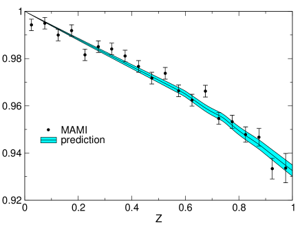
Figure 1: Prediction obtained from the KLOE measurements of $\eta\to\pi^{+}\pi^{-}\pi^{0}$ compared with the MAMI results for $\eta\to 3\pi^{0}$ ($Z\equiv X^{2}+Y^{2}$ represents the square of the distance from the center of the Dalitz plot).

The figure shows that the resulting $Z$-distribution is in excellent agreement with the MAMI data Prakhov+2009 . Quantitatively, the comparison yields $\chi^{2}=22.5$ for 20 data points (no free parameters).

This solves a long-standing puzzle: $\chi$PT predicts the slope $\alpha$ of the Z-distribution to be positive at one loop, while the measured slope is negative. The problem arises because $\alpha$ is tiny – estimating the uncertainties inherent in the one-loop representation with the rule given above, we find that the error in $\alpha$ is so large that not even the sign can reliably be determined. The situation does not improve at NNLO Bijnens+2007 . Only with dispersion theory is one able to reach the necessary precision and to reliably predict the slope.

At the precision at which the slope is quoted by the PDG, $\alpha_{\mathrm{PDG}}=-0.0315(15)$ Agashe:2014kda , the definition of $\alpha$ matters, because the $Z$-distribution is well described by the linear formula $1+2\hskip 0.85358pt\alpha\hskip 0.28453ptZ$ only at small values of $Z$. For the slope at $Z=0$, we find $\alpha=-0.0302(11)$, while a linear fit on the intervals $0<Z<0.5$ and $0<Z<1$ yields the slightly different values $\alpha=-0.0293(11)$ and $\alpha=-0.0313(11)$, respectively.

The decay rates of the processes $\eta\to\pi^{+}\pi^{-}\pi^{0}$ and $\eta\to 3\pi^{0}$ are given by an integral over the square of the corresponding amplitudes and hence by a quadratic form in the subtraction constants. For the individual rates, $H_{0}$ is also needed – and will be discussed below – but in the branching ratio $B=\Gamma(\eta\to 3\pi^{0})/\Gamma(\eta\to\pi^{+}\pi^{-}\pi^{0})$ the normalization drops out. The uncertainties in the dispersive representation also cancel almost completely. The error in our result, $B=1.44(4)$, is dominated by the uncertainties in the one-loop approximation used for isospin breaking. The comparison with the experimental values given by the Particle Data Group, $B=1.426(26)$ [‘our fit’], $B=1.48(5)$ [‘our average’] shows that the value predicted for the decay rate of the neutral mode (on the basis of Dalitz plot distribution and decay rate of the charged mode) agrees with experiment. This provides a very strong test of the approximations used to account for isospin breaking.

In contrast to the Dalitz plot distributions and the branching ratio, the individual rates do depend on the normalization of the amplitude, which we specify in terms of $(M_{K^{0}}^{2}-M_{K^{+}}^{2})_{\mathrm{QCD}}$ and $H_{0}$. With the theoretical estimate for $H_{0}$ given above, the experimental values of the rates $\Gamma(\eta\to\pi^{+}\pi^{-}\pi^{0})=300(12)$ eV and $\Gamma(\eta\to 3\pi^{0})=428(17)$ eV Agashe:2014kda yield two separate determinations of the kaon mass difference in QCD. Since our prediction for the branching ratio agrees with experiment, the two results are nearly the same, but they are statistically independent only with regard to the uncertainties in the rates, which are responsible for only a small fraction of the error. Combining the two, we can determine the mass difference to an accuracy of 6%:

$$(M_{K^{0}}^{2}-M_{K^{+}}^{2})_{\mathrm{QCD}}=6.27(38)10^{-3}\,\mbox{GeV}^{2}\,.$$ (11)

The comparison with the observed mass difference implies $(M_{K^{0}}^{2}-M_{K^{+}}^{2})_{\mathrm{QED}}=-2.38(38)10^{-3}\,\mbox{GeV}^{2}$. The corresponding result $\epsilon=0.9(3)$ for the parameter used to measure the violation of the Dashen-theorem Aoki:2016frl , agrees with recent lattice results Fodor:2016bgu ; Basak:2016jnn which also indicate that this theorem picks up large corrections from higher orders. Indeed, the direct determination of $\epsilon$ based on an evaluation of the kaon mass difference with the e.m. effective Lagrangian encounters unusually strong logarithmic infrared singularities, which generate large nonleading terms in the chiral perturbation series Langacker:1974nm . We emphasize that our determination of $\epsilon$ does not face this problem.

Finally, we invoke the low energy theorem that relates the kaon mass difference to the quark mass ratio $Q$ Gasser+1985a :

$$(M_{K^{0}}^{2}-M_{K^{+}}^{2})_{\mathrm{QCD}}=\frac{M_{K}^{2}(M_{K}^{2}-M_{\pi}^{2})}{Q^{2}M_{\pi}^{2}}\,,$$ (12)

($M_{K}$ and $M_{\pi}$ stand for the QCD masses in the limit $m_{u}=m_{d}$). Since the relation holds up to corrections of NNLO, our analysis goes through equally well if the quantity $(M_{K^{0}}^{2}-M_{K^{+}}^{2})_{\mathrm{QCD}}$ is replaced by the right hand side of (12). This leads to

$$Q=22.0(7)\,,$$ (13)

in good agreement with the values obtained on the lattice Aoki:2016frl . Using the remarkably precise result for the ratio $m_{s}/m_{ud}=27.30(34)$ quoted in the same reference, we can finally also determine the relative size of the two lightest quark masses: $m_{u}/m_{d}=0.44(3)$. The theoretical estimates for $H_{0},h_{1},h_{2},h_{3}$ and the experimental uncertainties in Dalitz plot distribution and rate contribute about equally to the quoted error in this determination of the isospin breaking quark mass ratios, while the uncertainties due to the noise in the $\pi\pi$ phase shifts are negligibly small. We defer a detailed discussion and a comparison with related work Bijnens+2007 ; Gullstrom:2008sy ; Schneider+2011 ; Kampf+2011 ; Guo:2015zqa ; Albaladejo+2015 ; Kolesar:2016jwe ; Guo:2016wsi to a forthcoming publication CLLP .

- (1) D. G. Sutherland, Phys. Lett. 23, 384 (1966)
- (2) H. Osborn and D. J. Wallace, Nucl. Phys. B20, 23 (1970)
- (3) J. Gasser and H. Leutwyler, Nucl. Phys. B250, 465, 539 (1985)
- (4) J. Bijnens and K. Ghorbani, JHEP 11, 030 (2007), arXiv:0709.0230
- (5) N. N. Khuri and S. B. Treiman, Phys. Rev. 119, 1115 (1960)
- (6) C. Roiesnel and T. N. Truong, Nucl. Phys. B187, 293 (1981)
- (7) A. V. Anisovich, Phys. Atom. Nucl. 58, 1383 (1995)
- (8) A. V. Anisovich et al., Three-particle physics and dispersion relation theory (World Scientific, Singapore, 2013)
- (9) A. V. Anisovich and H. Leutwyler, Phys. Lett. B375, 335 (1996), hep-ph/9601237
- (10) J. Kambor, C. Wiesendanger, and D. Wyler, Nucl. Phys. B465, 215 (1996), hep-ph/9509374
- (11) G. Colangelo, J. Gasser, and H. Leutwyler, Nucl. Phys. B603, 125 (2001), hep-ph/0103088
- (12) S. Descotes-Genon, N. H. Fuchs, L. Girlanda, and J. Stern, Eur. Phys. J. C24, 469 (2002), hep-ph/0112088
- (13) R. Kaminśki, J. R. Peláez, and F. J. Ynduráin, Phys. Rev. D77, 054015 (2008), arXiv:0710.1150
- (14) C. O. Gullström, A. Kupść, and A. Rusetsky, Phys. Rev. C79, 028201 (2009), arXiv:0812.2371
- (15) S. P. Schneider, B. Kubis, and C. Ditsche, JHEP 02, 028 (2011), arXiv:1010.3946
- (16) K. Kampf, M. Knecht, J. Novotný, and M. Zdráhal, Phys. Rev. D84, 114015 (2011), arXiv:1103.0982
- (17) S. Lanz, PoS CD12, 007 (2013), arXiv:1301.7282
- (18) P. Guo, I. V. Danilkin, D. Schott, C. Fernández-Ramírez, V. Mathieu, and A. P. Szczepaniak, Phys. Rev. D92, 054016 (2015), arXiv:1505.01715
- (19) P. Guo, I. V. Danilkin, C. Fernández-Ramírez, V. Mathieu, and A. P. Szczepaniak arXiv:1608.01447
- (20) M. Albaladejo and B. Moussallam, PoS CD15, 057 (2015)
- (21) M. Kolesár and J. Novotný arXiv:1607.00338
- (22) C. Ditsche, B. Kubis, and U.-G. Meißner, Eur. Phys. J. C60, 83 (2009), arXiv:0812.0344
- (23) G. Colangelo, S. Lanz, H. Leutwyler, and E. Passemar, in preparation
- (24) G. Colangelo, E. Passemar, and P. Stoffer, Eur. Phys. J. C75, 172 (2015), arXiv:1501.05627
- (25) J. A. Cronin, Phys. Rev. 161, 1483 (1967)
- (26) A. Anastasi et al. (KLOE-2), JHEP 05, 019 (2016), arXiv:1601.06985
- (27) F. Ambrosino et al. (KLOE), JHEP 05, 006 (2008), arXiv:0801.2642
- (28) P. Adlarson et al. (WASA-at-COSY), Phys. Rev. C90, 045207 (2014), arXiv:1406.2505
- (29) M. Ablikim et al. (BESIII), Phys. Rev. D92, 012014 (2015), arXiv:1506.05360 [hep-ex]
- (30) S. Prakhov et al. (Crystal Ball at MAMI), Phys. Rev. C79, 035204 (2009), arXiv:0812.1999
- (31) K. A. Olive et al. (Particle Data Group), Chin. Phys. C38, 090001 (2014)
- (32) S. Aoki et al., FLAG review, arXiv:1607.00299
- (33) Z. Fodor, C. Hoelbling, S. Krieg, L. Lellouch, T. Lippert, A. Portelli, A. Sastre, K. K. Szabo, and L. Varnhorst, Phys. Rev. Lett. 117, 082001 (2016), arXiv:1604.07112
- (34) S. Basak et al. (MILC), PoS LATTICE2015, 259 (2016), arXiv:1606.01228
- (35) P. Langacker and H. Pagels, Phys. Rev. D8, 4620 (1973)