Complexity and Stop Conditions for NP as General Assignment Problems, the Travel Salesman Problem in $\mathbb{R}^{2}$, Knight Tour Problem and Boolean Satisfiability Problem

Abstract

This paper presents stop conditions for solving General Assignment Problems (GAP), in particular for Travel Salesman Problem in an Euclidian 2D space the well known condition Jordan’s simple curve and opposite condition for the Knight Tour Problem. The Jordan’s simple curve condition means that a optimal trajectory must be simple curve, i.e., without crossing but for Knight Tour Problem we use the contrary, the feasible trajectory must have crossing in all cities of the tour. The paper presents the algorithms, examples and some results come from Concorde’s Home page. Several problem are studied to depict their properties. A classical decision problem SAT is studied in detail.

Keywords: Algorithms, TSP, NP, Numerical optimization.

1 Introduction

Building software is similar to prove theorems, i.e., to study, think, plan, revise, correct, cut, change, understand in order to pursuing an esthetic beauty for an efficiency procedure for solving questions or problems. I prefer constructivism on mathematical model, properties, theories over heuristic or recipes. The NP problems [18] and the 2D Euclidian Traveller Salesman (hereafter, TSP) have been studied abroad. The Combinatorics and Optimization Department of the University of Waterloo has made an splendid research and offer free software for TSP (the Concorde software [1]).

This paper complement my previous papers [10, 11] in the study of relationship between the class NP and the class P.

Here, I present a carefully study of the properties of similar problems TSP, Knight tours problem (KTP), polygonals (as TSP type), and Boolean Satisfiability Problem (SAT).

For TSP and KTP, there are abroad articles and publications, I mentions two for my preference, of course other are quite important:  [4, 19, 20].

The property of a Jordan’s simple curve is for the first time used for developing an efficient algorithm. The Jordan’s simple curve come from [4] figures 1.21 and 1.22 (pag. 24) as uncrossing the tour segments. To my knowledge, what makes different my novel approach (using Jordan’s simple curve) is the combination of visualization data techniques with a very simple optimization algorithms using greedy and uniform search strategies and the study of mathematical properties for understanding stop conditions and when they are necessary or sufficient. This means that optimization program are polynomial time when the search space for TSP is convex but yes-no program for GAP_nin general could have a large research space without an appropriate data organization, therefore there is not polynomial time algorithm for answering them.

In general, for the TSP under euclidian distance (or where the coseno law states) Jordan’s simple curve is a necessary condition on a plane but sufficient. This is similar to solve by the necessary condition $f^{\prime}(x)=0$, an global optimization problem with objective function $f$, which is derivable. This is the well known first order necessary condition in optimization. It does not imply the optimality. To be sufficient it is needed, by example, that $f$ must be quadratic or convex. For the TSP, Jordan’s simple curve condition provides a stop condition (necessary condition, see Prop. 4.3) to build an approximation to the solution and with other geometrical properties as convexity, it becomes a necessary and sufficient condition (see Prop. 4.4).

I include some parts to make this paper self-explicatory from my papers [10, 11].

2 Travel Salesman Problem, and Knight Tour Problem like General Assign Problem

The well known Travel Salesman Problem (TSP) and Knight Tour Problem (KTP) are particular cases of the General Assign Problem(GAP), some properties and characteristics are  [10].

The GAP_n consists a complete graph, a function which assigns a value for each edge, and objective function, $\text{GAP}\_n$ $=$ $(G_{n},c,f)$, where $G_{n}=\left(V_{n},A\right)$, $V_{n}$ $\subset$ $\mathbb{N}$ $A$ $=$ $\left\{\left(i,j\right)\,|\,i,j\in V\right\}$, $c:V\times V\rightarrow\overline{\mathbb{R}}$, and $f$ is a real function for the evaluation of any path of vertices.

In particular, without lost of generality, I focus in minimization to solving a GAP. It means to look for a minimum value of $f$ over all hamiltonian cycles of $G_{n}$. Also, it is trivial to see that any GAP_n has a solution.

The main proposition in  [10], it depicts contradictory properties and characteristics for solving GAP_n:

Proposition 6.12. An arbitrary and large GAP_n of the NP-Class has not a polynomial algorithm for checking their solution.

In this article, SAT_n×m is used to state:

Proposition 9.9. SAT_n×m has not property or heuristic to build an efficient algorithm.

Proposition 9.10. NP has not property or heuristic to build an efficient algorithm.

In my previous articles, I did not give an explication of why I selected graph as the main core of my study. From the [13]: ”Euler called this new mathematics without numbers, in which only the structure of the configuration plays a role, but not size and form, Geometria situs, geometry of position (he took the concept from a letter of Leibniz from the year 1679).” Methods for solving the NP look for a common, and global property but using graphs, they depict local properties, i.e., properties related to immediately vicinity of the nodes. Therefore, what is valid in a situs could be invalid in other positions. Here, on the other hand, a simple tipo of SAT_n is studied to support that there is not a property to build an efficient algorithm to avoid an exhaustive searching of the search space or to let to build knowledge from a polinomial population of cases.

The travel salesman problem with cities as points in a $m$-dimensional euclidian space (TSP_n) is a special case of a GAP_n where the edge’s cost is given by the matrix $\mathcal{C}=\left[c(i,j)\right],c\left(i,i\right)=\infty,i=1,\ldots,n,j=1,\ldots,n.$ $c(i,j)=\hbox{euclidian distance}(i,j)$ $\forall i\neq j\in V_{n}$, and the vertex $i$ is a point in $\mathbb{R}^{m},m\geq 2$. The elements of the diagonal of $\mathcal{C}$ are equals to $\infty$, this is to avoid getting stuck. TSP2D (Hereafter, TSP) is a problem with cities as points in $\mathbb{R}^{2}$ and edges’s values come from their euclidian distances between cities.

In similar way, the Knight tour problem (hereafter, KTP) is an special special case of a GAP_n where the vertices are fixed in each square’s center of a chessboard $n\times m$. The squares’coordinate are given by their integer coordinates of the chessboard’s squares. The edge’s cost is given by the matrix C $=\left[c(i,j)\right],c\left(i,i\right)=\infty,\hbox{Euler distance}(i,j)$ $\forall i\neq j$. To honor the great Mathematician Leonard Euler, I called it as Euler’s distance (see  [20]).

$\hbox{Euler's distance}(i,j)=\left\{\begin{array}[]{ll}c_{1}&\text{if }\left(i-i^{\prime}\right)^{2}+\left(j-j^{\prime}\right)^{2}=5\\ \infty&i=j\\ \sqrt{\left(\left(i-i^{\prime}\right)^{2}+\left(j-j^{\prime}\right)^{2}\right)}+4&\text{otherwise}\end{array}.\right.$

My first approach was select $c_{1}=0.01$. However, in order to privilege the knight moves, $c_{1}$ needs a more carefully tuning (see section 5). The problem consists to look for a hamiltonian cycle in a chessboard of $8\times 8$ with cost less than 4.

The  [19] depicts in chapters 40 through 42 results about uncrossed, celtic, long and skinny knight’s tours.

The following propositions are known, I include for clarity.

Proposition 2.1.

Any TSP is soluble, i.e. there is a minimum cost hamiltonian cycle.

Proof.

It obvious, a TSP has n cities, and its a complete graph. Then by comparing the all (n-1)! hamiltonian cycles the solution is found. ∎

Proposition 2.2.

A graph knight is a graph $m$ $\times$ $n$ squares if only if $\forall mn$ vertices $(i,j)$, $(i^{\prime},j^{\prime})$ with $1\leq i<i^{\prime}\leq m,$ and $1\leq j<j^{\prime}\leq n$, the square distance, $\left(i-i^{\prime}\right)^{2}+\left(j-j^{\prime}\right)^{2}=5$.

Proof.

See [19]. A knight walks in a chessboard in L form from a white square to a black square. In order, for a knight moving around all vertices, they need to be adjacent vertices to allowable the motion of the knight. ∎

Remark 2.3.

For the TSP and KTP we are interesting to find a minimum hamiltonian cycle.

However, the previous proposition does not considere exactly KTP, a hamiltonian cycle with only knight´s move but hamiltonian path.

The idea of the Euler distances function come from the previous proposition to provide space and to favor the moves of a knight. Some results from  [19] can be verified by doing exhaustive search. I create a a simple Matlab programs to verify some knight’s tour in small chessboards (if you want a copy, email me).

From the last two propositions, I define what type solutions to focus in this paper:

1. for the TSP, a minimum cost hamiltonian cycle, and

2. for the KTP a crossing hamiltonian cycle with only knight´s move.

The TSP correspond to calculate and prove the optimality and for the KTP is to find a special hamiltonian cycle.

They are quite different. Nevertheless, for any objective function $f$ of a GAP_n, hamiltonian’s path or cycle are computable problems and the minimum selection procedure could be used to find the solution (see proposition 3.2 in  [10]). The minimum selection procedure in mathematical notation is:

$$y^{\ast}=\arg\min_{y=(v_{1},v_{2},\ldots,v_{n},v_{1}),v_{1}\in V_{n},v_{i}\in V_{n},v_{i}\neq v_{j},1\leq i<j\leq n}\left\{f(y)\,|\,\hbox{GAP}_{n}=(G_{n},c,f),G_{n}=(V_{n},A)\right\}$$ (2.1)

It is clear that both TSP and KTP are GAP${}_{n}^{\prime}$s type with a similar type of an objective function, $f,$ which is the summation of the edges’ cost over the consecutive pairs of vertices of a path. However, TSP is a hard NP problem, similar to a global optimization problem. On the other hand, KTP is a decisión problem to look for a crossing hamiltonian cycle.

The Research Space of GAP_n is finite and numerable, and it has $(n-1)!$ elements (see Prop.3.4  [10]). It is totally impractical, to solve eq. 2.1 by an exhaustive searching procedure.

3 A greedy algorithm for Eq. 2.1

Algorithms for solving global optimization problems have abundant literature. For arbitrary objective functions on a bounded subset, $B\subset\mathbb{R}^{m}$, uniform searching combined with local optimization can be used to estimate the global optimal solution (see Theorems of Convergence: Global and Local Search in [21]). The convergence to the solution has not guaranty of polynomial time complexity and the solution can be found at the cost of thoroughly searching on $B$. This motivate to create heuristic methods, by example, I worked in heuristic methods:

1. Classical and Exponential Tunnelling method [5, 16, 17]. These methods do not guaranty to find the global solution but a descend of the objective function’s value. The user defines and decides the number of iterations or the time’s execution.

2. Genetic Algorithms for Global Optimization for the LJ Problem [6, 7, 9].

The following heuristic greedy algorithm execute an uniform search on the vertices, or select the closed vertex, and repeat this procedure $K$ times ($K>>0$):

Algorithm 1.

Input: GAP_n with $\mathcal{C}=\left[c(i,j)\right],$ matrix of the edge’s cost, a hamiltonian cycle, $V_{o}=(v_{1},v_{2},\ldots,v_{n},$ $v_{1})$, with minimum cost $c_{o}$.

Output: $v_{o}=(v_{1},v_{2},\ldots,v_{n},v_{1})$ a hamiltonian cycle with minimum cost $c_{o}.$

1. For $r=1$ to $K$

2. Select randomly an initial vertex by column or row $i_{v}$, or $j_{v}$ from $1\leq i_{v},j_{v}\leq n$.

3. $j_{v}=\arg min_{1\leq j\leq n}\left[c(i_{v},j)\right]$   or $i_{v}=\arg min_{1\leq i\leq n}\left[c(i,j_{v})\right];$

4. $v_{1}$ = $i_{v}$ or $j_{v}$;

5. end select

6. $i=1;$

7. $V_{a}=(v_{1})$.

8. While $V_{a}$ is not a hamiltonian path

9. $v_{i+1}=$ Select randomly $\left\{\begin{array}[]{c}\arg min_{1\leq j\leq n}\left[c(v_{i},j)\right]\\ \mathbf{Selectrandomly\ }v_{j}\notin v_{a}\end{array}\right.;$

10. if $v_{i+1}$ $\notin$ $V_{a}$   then

11. add $v_{i+1}$ to $V_{a};$

12. else

13. $i=mod(i+1,n)+1;$

14. end if

15. end while

16. $V_{a}=(v_{1},v_{2},\ldots,v_{n},v_{1});$

17. $c_{a}=f(V_{a});$

18. if $c_{a}<c_{o}$ then

19. $V_{o}=V_{a};$

20. $c_{o}=c_{a};$

21. end if

22. end for $r$

Remark 3.1.

A putative minimum hamiltonian cycle can be obtained by the previous algorithm. Or it keeps the current putative minimum hamiltonian cycle. The value of $K$ is $200$.

To behave only greedy the step 9 could be changed to $v_{i+1}=$ $\arg min_{1\leq j\leq n}\left[c(v_{i},j)\right]$. And reciprocally, to set on uniform search this step could be changed to $v_{i+1}=$ $\mathbf{Select\ randomly\ }v_{j}\notin v_{a}$

4 Algorithm for TSP

Prop. 6.11 in  [10] depicts that for any quadrilateral, its sides are lower than its diagonal. This section depicts algorithms for solving TSP using this property.

Algorithm 5 in  [10] is used to order the vertices according to a given hamiltonian cycle. Hereafter, we assume that the current hamiltonian cycle is in ascending order of the consecutive cities. It is not necessary, but assuming that the vertices of the hamiltonian cycle are in order facilitate the description of the following algorithms.

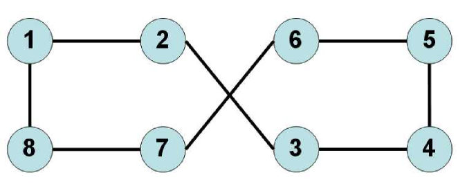
Figure 1: Hamiltonian cycle with a crossing in the cities: $v_{2},v_{3},v_{6},v_{7}.$

Let’s assume that with algorithm 1, there is a hamiltonian cycle for a given TSP. An image of the current solution can be obtained by a graphic interface as in Concorde or using the graphic’s tool of Matlab or Octave. By example see fig. 1.

Algorithm 2.

Input: An black and white image of the current hamiltonian cycle, $v=(v_{1},v_{2},\ldots,v_{n},v_{1})$ where the cities are in order consecutive.

Output: Stop, the image of the hamiltonian cycle can be colored by two colors. Otherwise, the hamiltonian cycle has a crossing at the cities $v_{i},v_{i+1},v_{j},v_{j+1}$.

1. Using $v_{1}$ detects its location in the input image.

2. Using $v_{1}$ detects its frontier in the image for selecting two points, one inside and one outside of the $v_{1}$.

3. Using a flood or a paint graphic tool with the point outside of the $v_{1}$, colored the image on green.

4. Using a flood or a paint graphic tool with the point inside of the $v_{1}$, colored the image of red.

5. two_color=”yes”;

6. for $i:=1$ to $n$

7. Using $v_{i}$ detects its location in the colored input image;

8. if the vicinity of the $v_{i}$ has red, green and black then

9. continue;

10. else

11. two_color=”no”;

12. mark $v_{i};$

13. end for $i;$

14. if  two_color is ”yes” then

15. Stop. ”The image of the hamiltonian cycle can be colored by two colors,$v=(v_{1},v_{2},\ldots,v_{n},v_{1})$ is a hamiltonian cycle as Jordan’s simple curve, i.e., without crossing.”;

16. select marked vertex, let assume it is $v_{i}$

17. using $v_{i}$ detects its location in the colored input image;

18. using $v_{i}$ detects its four closed marked neighbors;

19. Stop. There is crossing at the cities: $v_{i},v_{i+1},v_{j},v_{j+1}$.

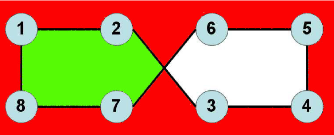
Figure 2: Colored image of a hamiltonian cycle with a crossing in the cities: $v_{2},v_{3},v_{6},v_{7}.$

Remark 4.1.

Flood or paint graphic tool algorithm has the complexity of the image’s size is $\mathbf{O}(kn^{2})$ where $kn$ is related to the resolution of the vicinity of the $n$ vertices. The value of factor $k$ depends of the minimum distance of the vertices. $k$ must be allow to have a black-white image where the lines of hamiltonian cycle are clearly distinguish. Figure  2 depicts when there is a crossing.

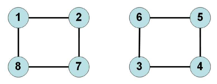
Figure 3: Wrong connection of crossing in the cities: $v_{2},v_{3},v_{6},v_{7}.$

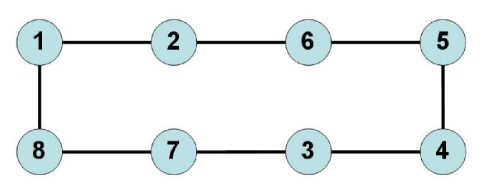
Figure 4: Hamiltonian cycle without the crossing in the cities: $v_{2},v_{3},v_{6},v_{7}.$

Assuming that vertices of the hamiltonian cycle are in order, the only one solution for figure 2 is depicted in figure 4. Figure 3 depicts the wrong connection. There are two possibilities when a crossing is found, but only one is the correct on the current hamiltonian cycle. Nevertheless, the cost of the cycle always decreases. Therefore, if there is crossing at the cities $v_{i},v_{i+1},v_{j},v_{j+1}$ the hamiltonian cycle must connects $v_{i}$ to $v_{j}$ and $v_{i+1}$ to $v_{j+1}$ and there is always a guaranty for decreasing cycle’s cost from Prop. 6.11 in  [10].

Without loss of generality, let’s assume that $i<j$.

Algorithm 3.

Input: $V=(v_{1},v_{2},\ldots,v_{n},v_{1})$ a hamiltonian cycle, where the cities are in order consecutive and with a crossing in four cities: $v_{i},v_{i+1},v_{j},v_{j+1}.$

Output: $V=(v_{1},v_{2},\ldots,v_{n})$ a hamiltonian cycle without the crossing at the cities $v_{i},v_{i+1},v_{j},v_{j+1}.$

1. $V^{\prime}=V;$

2. $l=j$

3. for k:= i+1 to j

4. $V(k)=V^{\prime}(l)$

5. $l=l-1;$

6. end for $k;$

7. stop. The hamiltonian cycle without the crossing is $V=(v_{1},v_{2},\ldots,v_{i},v_{j},v_{j-1},\ldots,v_{i+1},v_{j+1},\ldots,v_{n},v_{1})$.

Remark 4.2.

The complexity of the previous algorithm is $\mathbf{O}(n)$. The next steps are for ordering the cities of the hamiltonian cycle, perhaps to repeat a greedy algorithm for looking a less hamiltonian cycle’s cost around the current solution. The next paragraph depicts the complete algorithm for solving the TSP, using the previous algorithms to get a simple Jordan’s simple curve. This is a necessary condition to stop, because the crossing of the cities is a visual property for detecting where the hamiltonian cycle’s cost decreases.

Algorithm 4.

Input: TSP.

Output: $V=(v_{1},v_{2},\ldots,v_{n},v_{1})$ a hamiltonian cycle as Jordan’s simple curve, i.e., without any crossing on the path of cities.

1. Repeat

2. execute algorithm 1;

3. execute algorithm 5 in  [10] to order the hamiltonian cycle by their consecutive cities;

4. create a black-white image;

5. execute algorithm 2

6. until get a Jordan’s simple curve from the current hamiltonian cycle.

7. Stop. The hamiltonian cycle is the putative solution of the TSP.

Proposition 4.3.

Given a TSP_n, where cities are points in $\mathbb{R}^{2}$, and the cost matrix correspond to euclidian distances between cities. The Jordan’s simple curve is a necessary condition for the minimum hamiltonian cycle’s cost.

Proof.

With out loss of generality, if the putative optimal hamiltonian cycle has a crossing then for Prop. 6.11 in  [10], the hamiltonian cycle obtained by algorithm 3 has lower value than the putative optimal hamiltonian cycle. ∎

Proposition 4.4.

Given a TSP_n, if cities are located around a closed convex curve, the algorithm  4 finds the hamiltonian cycle of minimum cost.

Proof.

The optimality of the hamiltonian cycle comes from the vertices’configuration around of convex curve, points on a circle, elipse, n-poligonal. The algorithm 1 by construction selects the closed next vertex. The hamiltonian cycle corresponds to the solution of the variational problem of the the minimum length s curve (Jordan’s simple curve) with the maximum convex area. ∎

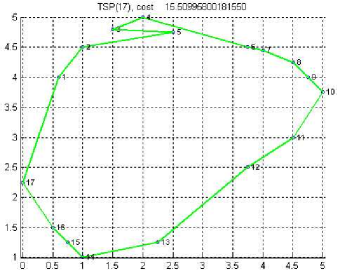
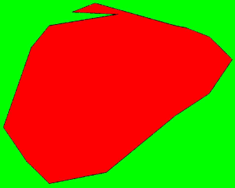
a) b)

Figure 5: TSP₁₇. a) Not optimal hamiltonian cycle with Jordan’s simple curve, and b) its two colored image.

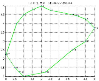
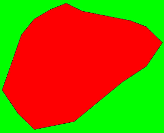
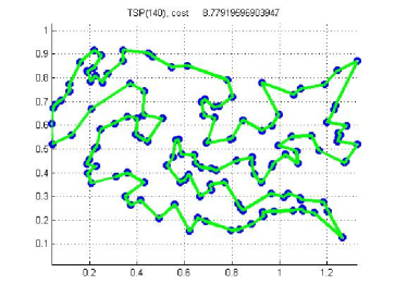
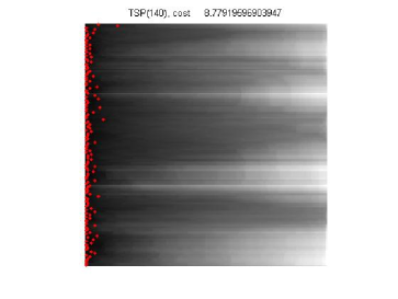
a) b)

Figure 6: TSP₁₇. a) Optimal hamiltonian cycle with Jordan’s simple curve, and b) its two colored image.

a) b)

Figure 7: TSP₁₄₀. a) Hamiltonian cycle with the minimum cost, and b) sorted cost matrix $\mathcal{M}$. The red dots on the left side implies that there are not many alternatives hamiltonian cycles.

Remark 4.5.

Figure 5 depicts a case where the algorithm 2   fails to detect the zone where it is possible to descend the cost. However, there are many algorithms where this not happen. I hope, that the algorithms of the Concorde [1] for TSP2D get advantage of the Jordan’s simple curve property in the future.

Unfortunately, for TSP where the objective is to get a minimum hamiltonian cycle’s cost related to money, time travel or arbitrary values then Jordan’s simple curve property is not useful. This includes the max distance giving by: $d_{m}(x,y)=\max\{|x_{1}-y_{1}|,|x_{2}-y_{2}\ \},$ where $x=(x_{1},x_{2}),$ and $y=(y_{1},y_{2})\in\mathbb{R}^{2}$. It is easy to verify that a quadrilateral under $d_{m}$ has diagonals not larger than its sides.

Figures 5 and 6 depict a case where the previous proposition is verified for a small TSP₁₇. Red area of the former figure has $415,570$ pixels with cost = $15.5100$, and red area of next figure has $417,719$ pixels with cost = $13.5849$. Also, these figures shows why the Jordan’s simple curve is a necessary property.

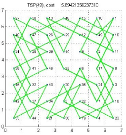
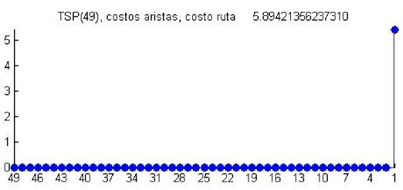
a) b)

Figure 16: TKP_7×7. a) final tour, and b) edges’cost.

Using algorithm 4, big TSP can be solved to a putative optimal hamiltonian cycle. Figure 7 taken from  [10] (Figure 16) depicts a Jordan’s simple curve. The red dots depicts the minimum hamiltonian cycle, it corresponds to vertices’ enumeration closed to the left side. In this case the complexity of the algorithm 4 until getting a Jordan’s simple curve is polinomial time bounded by $\mathbf{O}(n^{k})$ with $k$ a small positive integer, and the time depends of the many crossings that the greedy algorithm 1 can to avoid.

5 Algorithm for KTP

The Euler’s distance of the KTP does not connect the squares of a chessboard as usual, but it privilege the knight’s moves. It is clear that Prop. 6.11 in  [10] (sides versus diagonals of quadrilaterals) can not be used for solving KTP, i.e., the algorithm for the KTP is looking for the contrary of a simple Jordan’s simple curve as in TSP, in fact, the property is a hamiltonian cycle with many crossing as possible.

The algorithm 1 is used without a modification. But, here the goal is to stop when the cost of the hamiltonian cycle is less than $4.$

To my knowledge there is not a proposition or theorem for proving that exists a complete crossing knight tour for any chessboard’s size. In [2] there is a table of solutions for some chessboard’s size. I tune the Euler’s distance function using the description of the article [20]. The knight’s motion has three different behaviors each quadrant of size $4\times 4$:

1. Two romboides with direction $(-1,-1)$ to $(1,1)$;

2. Two romboides with direction $(-1,1)$ to $(1,-1)$;

3. Two squares.

Algorithm 5.

Input: KTP for a chessboard of $8\times 8$.

Output: $V=(v_{1},v_{2},\ldots,v_{n},v_{1})$ a hamiltonian cycle with cost less than 4.

1. Execute algorithm 1.

2. while current hamiltonian cycle’s cost $\geq$ 4 do

3. execute algorithm 5 in  [10] to order the hamiltonian cycle by their consecutive vertices;

4. execute algorithm 1;

5. end while.

6. Stop. The hamiltonian cycle is the solution of the KTP.

There is not guaranty that the previous algorithm is computable, i.e., it could not to stop for an arbitrary chessboard’s size. I mean that the tuning of $c_{1}$ works for a chessboard of $8\times 8$. For arbitrary chessboard’s size, it could not provide a hamiltonian path because the corresponding GAP could not have a hamiltonian cycle with cost less than $4$.

The selection of the value $4$ is in the hope that the greedy part of the algorithm 1’s behaves greedy when it searches for minimum hamiltonian cycle’s cost. It will prefer to choice edge’s cost between vertices that corresponds knight’s paths. By construction the total distance of a tour with only knight’s motion is less than $4.$ For any pair of squares that not correspond to knight’s paths the distance is giving by sqrt$\left(\left(i-i^{\prime}\right)^{2}+\left(j-j^{\prime}\right)^{2}\right)+4$, .i.e. when $\left(i-i^{\prime}\right)^{2}+\left(j-j^{\prime}\right)^{2}\neq 5$ where $(i,j)$ and $(i^{\prime},j^{\prime})$ are the integer coordinates of the squares.

For a knight’s paths the value of $c_{1}$ of the Euler’s distance is $0.04,$ but in each quadrant of size $4\times 4$ the value of $c_{1}$ is:

1. $0.01$ for the two romboides with direction $(-1,-1)$ to $(1,1);$

2. $0.03$ for the two romboides with direction $(-1,1)$ to $(1,-1);$

3. $0.02$ for the two squares.

a) b)

Figure 8: TSP₁₅₂ on a spiral. Two colored Jordan’s simple curve: a) not optimal hamiltonian cycle $21.1661$, and b) optimal hamiltonian cycle $21.1451$.

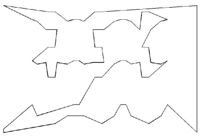
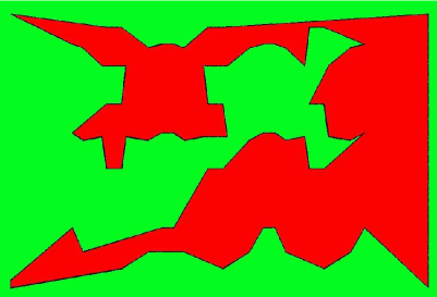
a) b)

Figure 9: TSP₇₆(file pr76.tsp). a) final hamiltonian cycle with Jordan’s simple curve, and b) its two colored image.

Figure 10: TSP₄₄₂(file pcb442.tsp). Final two colored hamiltonian cycle with cost = $56,601.1738.$

Remark 5.1.

The heuristic idea to assign $c_{1}$ values come from the article [20], and without any formal proof, it works for KTP $8\times 8$ using the GAP$\_n$’s algorithm 1.

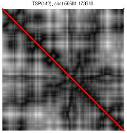
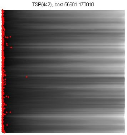
a) b)

Figure 11: TSP₄₄₂ final hamiltonian cycle. a) Ordered cost matrix, and b) sorted cost matrix $\mathcal{M}$.

6 Numerical Experiments for TSP and KTP

The first numerical experiment is for TSP with 152 cities located on a spiral curve. TPS₁₅₂. Figure 8 depicts two very closed hamiltonian cycles. On a) is the not optimal, its red area has $161,279$ pixels, and on b) is the putative optimal, its red area has $158,813$ pixels. The cost’s difference between the two hamiltonian cycles is only $0.021$. Also, the cities locations are not fulfil the hypothesis of proposition 4.4, therefore their red areas’size are not as in figures 5 and 6.

From [1] the files pr76.tsp and pcb442.tsp provide the results depicted on figures 9 and 10. The putative optimal complex hamiltonian cycle of the TSP₄₄₂ is not the global optimal. Figure 11 depicts on b) many red dots far away of the left side, as I explains in [10] this means that exists yet many alternatives hamiltonian cycles to explore. A rough estimation of this left research space’s size is $5.625417\times 10^{39}$ cycles. With the simple algorithm 4, I did not expect to solve this problem but to get a hamiltonian cycle less than initial cost of the $221435.5555$. The reduction of the cost is $164,834.3817$. Because, algorithm 2 is done by hand, the total time of execution can not be estimated.

Figures 12, and  16 depict solutions where all moves are knight’s path but one is not. The b) edge’s cost point out where there is not a knight’s move.

Proposition 6.1.

A KTP exists in any chessboard of $m$ $\times$ $n$ squares if only if $nm$ is even.

Proof.

A knight jumps from a white square to a black square. Therefore, in order to complete a hamiltonian cycle with only knight’s path, it is necessary to have equal number of white squares and black squares. ∎

Remark 6.2.

Proposition 2.2 states a very strong property but the verification is exhaustive. The previos proposition is easy to verify and together with prop. 2.2 it is immediately that for KTP in $n\times n$ chessboard, $n$ must be greater or equal 4, and even to guaranty the solution of KTP. A version of the previous proposition with black and white domino tiles, also requires $nm$ even in order to be tiling a $n\times m$ chessboard.

Therefore, for $5\times 5$ and $7\times 7$ chessboards there are not hamiltonian cycles with only knight’s path. Algorithm 5 is computable because it was designed for a chessboard $m$ $\times$ $n$ squares with $nm$, even. For clarity, prop. 2.2 states that hamiltonian trajectories exist in any knight graph. The prop. 2.2 and  6.1 are the kind of details that frequently happen in the design of efficient methods for instances of NP like problems. Previous knowledge, formal propositions, or heuristic ideas work very well for a instance problem or case, but, they do not work for similar and related problem. In order to solve, $5\times 5$ and $7\times 7$ chessboards repeat-end control structure for 200 times replaces the while-end in lines 2 through 5. The sorted cost matrix $\mathcal{m}$ in figures 13, and  17 b) depict that there are many similar solutions because not all red dots are on the left side. The value of the final cost in fig. 12, and  16 b) depict a hamiltonian trajectory omitting one edge. The cost values or the edge’s cost graphic are indicators to allow us the corroboration of the solution without additional computational cost.

a) b)

Figure 12: TKP_5×5. a) final tour, and b) edges’cost.

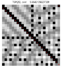
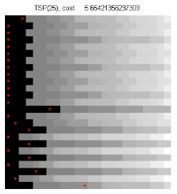
a) b)

Figure 13: TKP_5×5 of the final tour. a) Ordered cost matrix, and b) sorted cost matrix $\mathcal{M}$.

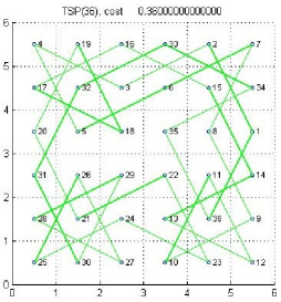
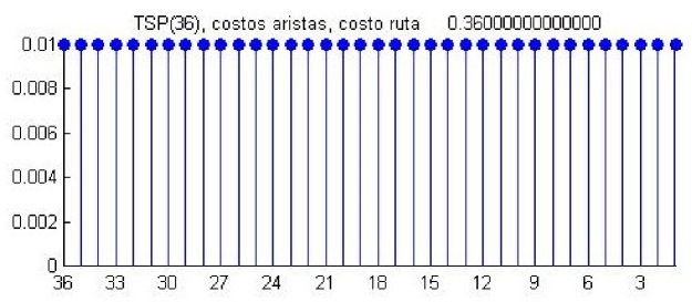
a) b)

Figure 14: TKP_6×6. a) final tour, and b) edges’cost.

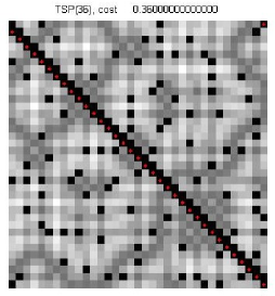
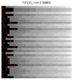
a) b)

Figure 15: TKP_6×6 of the final tour. a) Ordered cost matrix, and b) sorted cost matrix $\mathcal{M}$.

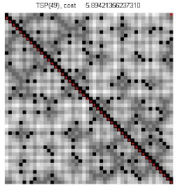
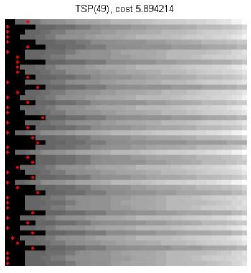
a) b)

Figure 17: TKP_7×7 of the final tour. a) Ordered cost matrix, and b) sorted cost matrix $\mathcal{M}$.

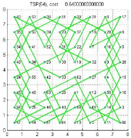
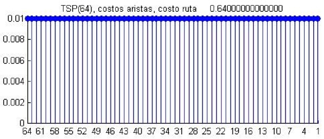
a) b)

Figure 18: TKP_8×8. a) final tour, and b) edges’cost.

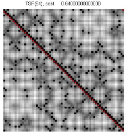
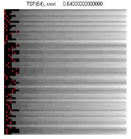
a) b)

Figure 19: TKP_8×8 of the final tour. a) Ordered cost matrix, and b) sorted cost matrix $\mathcal{M}$.

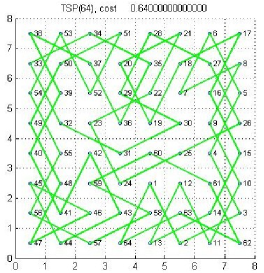
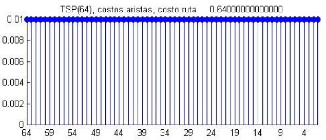
a) b)

Figure 20: TKP_8×8. a) final tour 2, and b) edges’cost.

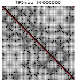
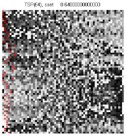
a) b)

Figure 21: TKP_8×8 of the final tour 2. a) Ordered cost matrix, and b) sorted cost matrix $\mathcal{M}$.

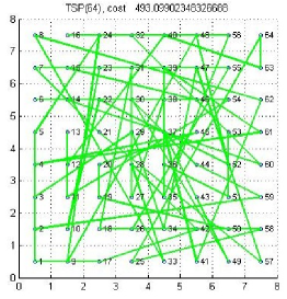
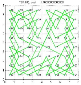
a) b)

Figure 22: TKP_8×8. a) Initial tour, and b) final tour with cost $<$ 4.

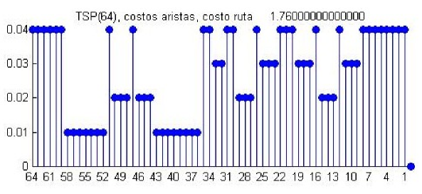
Figure 23: TKP_8×8. Edge’s cost depicts that they correspond only to knight’s motions for the final tour.

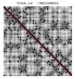
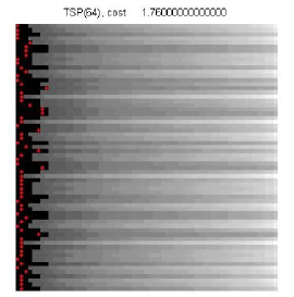
a) b)

Figure 24: TKP_8×8 of the final tour. a) Ordered cost matrix, and b) sorted cost matrix $\mathcal{M}$.

Figure 22 depicts the initial and final tour, and figure 23 depicts that the final tour corresponds only to knight’s paths, i.e., $\left(i-i^{\prime}\right)^{2}+\left(j-j^{\prime}\right)^{2}=5$ where $(i,j)$ and $(i^{\prime},j^{\prime})$ are the integer coordinates of the squares of the final hamiltonian cycle. For the figure 24 an heuristical estimation of the posibles alternatives or a rough estimation of the research space’s size is $29,030,400$.

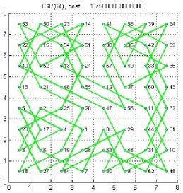
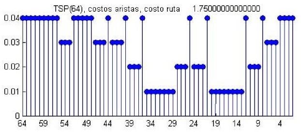
a) b)

Figure 25: TKP_8×8. a) final tour 2, and b) edges’cost.

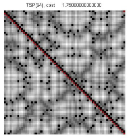
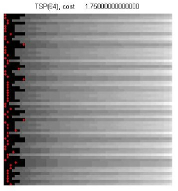
a) b)

Figure 26: TKP_8×8 of the final tour 2. a) Ordered cost matrix, and b) sorted cost matrix $\mathcal{M}$.

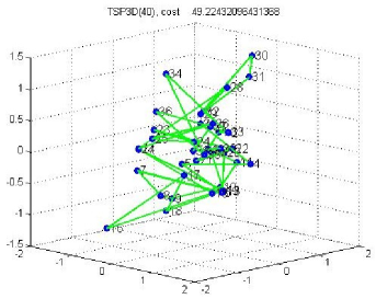
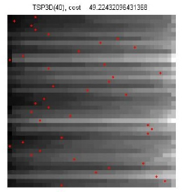
a) b)

Figure 27: TSP3D₄₀. a) Initial 3D Hamiltonian cycle, and b) sorted cost matrix $\mathcal{M}$. The red dots on the left side implies that there are many alternatives hamiltonian cycles.

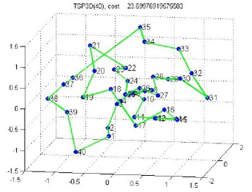
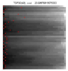
a) b)

Figure 28: TSP3D₄₀. a) Putative 3D Optimal hamiltonian cycle, and b) sorted cost matrix $\mathcal{M}$. The red dots on the left side implies that there are still many alternatives hamiltonian cycles.

7 Polygonal shapes and properties

This section depicts efficient algorithms using previous knowledge to replace the algorithm of section 3. It is clear that the population of the searching space for KTP or TSP problems are reduced when an algorithm focuses in appropriate properties. In fact, the next proposition follows trivially from the prop. 4.4.

Proposition 7.1.

Given a TSP_n where the cities are the vertex of a regular polygon in $\mathbb{R}^{2}$. Then the minimum Hamiltonian cycle is the polygon using Euclidian, $\max$, and abs distance.

A regular polygon has sides of the same length. Hereafter, regular polygon is named polygon.

An algorithm to state this obvious solution must be $\mathbf{O}(n)$. Figure 29 depicts an example of the polygon as TSP₅. This is by using the formulas $y_{i}=r\sin(2\pi i/n)$ and $x_{i}=r\cos(2\pi i/n),$ $i=0,\ldots,n-1$. The cost of minimum Hamiltonian cycle depends of the Euclidian, $\max$, or abs distance, but not the shape, which is always a Jordan’s simple convex curve.

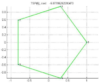
Figure 29: Pentagon as a TSP₅.

Polygon_n shape problem have a property to work for searching the minimum length, but what about the maximum length on cities as the vertex of a polygon of $n$ vertices in $\mathbb{R}^{2}$ using Euclidian, $\max$, and abs distance.

Hereafter, PoMX_n define the problem find the maximum distance of the vertices of a polygon of $n$ vertices using Euclidian (POME_n), $\max$ (POMm_n, or abs ((POMa_n) distance where X denotes E,m or a. Also, an star is a crossing Hamiltonian cycle over the vertices of a polygon with all angles equals.

Proposition 7.2.

Given a PoME_n where the cities are the vertex of a polygon in $\mathbb{R}^{2}$. Then the maximum Hamiltonian cycle is a star when $n$ is odd.

Proof.

First, assuming that the Hamiltonian cycle is a star, it has the maximum length under Euclidian distance because the secants corresponds to the diagonals of circumscribe triangles.

For $n$ odd, without loss of generality $n=2k+1$ for some $k\in\mathbb{N}$. The sequence $\left\{\left(1+\left(i-1\right)k\right)\text{mod}n\right\},$ $i=1,2,\ldots,n,n+1,$ form an star (crossing Hamiltonian cycle) for the vertices of the given polygon.

The function $s\left(i,k\right)=\left(1+\left(i-1\right)k,\left(1+\left(i-1\right)k\right)\text{mod}\left(2k+1\right)\right)$ computes a positive integer where the second entry is the residuos of $n$ or the congruent classes mod $n.$ For a given $k$, two consecutive numbers $1+\left(i-1\right)k$ and $1+\left(i\right)k$ are in different class mod $n.$ For $i=n+1=2k+2$, corresponds to the class 1 mod $n.$ And by construction all sequence numbers $1,1+k,\ldots,1+\left(i-1\right)k,$ $i=1,2,\ldots,n,n+1,$ are in different class mod $n$ except the first and the last one. ∎

For $n$ even under the Euclidian distance there is not a proposition as the previous but similar to a star when $n>>0$. In fact, for any $n$ even never is a star. Figure 32 depicts a no star.

For $n$ odd the symmetry allow to build an efficient algorithm under the Euclidian distance. Assuming that the vertices are numbered using the previous formulas for $(x_{i},y_{i})$, then $1,\left(1+\left(i-1\right)\frac{n-1}{2}\right)\text{mod}\left(n\right),\ldots,1$ defines a star. By example for $n=13$ the vertices of the star are $1,7,13(\text{or\ }0),6,12,5,11,4,10,3,9,2,8,$ and $1$ as is depicted in Fig. 30. Figure 33 depicts a star for POME₉₉.

On the other hand, POMa₁₃ and POMm₁₃ are no stars, they are depicted in Fig. 31 a) and b) respectively. These differences are caused by using $\max$ distance and abs distance instead Euclidian distance.

It is well know that an algorithm for minimization can be used for maximization using $-f$. However, geometry properties, as by example Simple Jordan’s curve is not preserve in maximization. Moreover, minimum length over a polygon is always a polygon. This previous knowledge defines a very efficient algorithm to build the minimum Hamiltonian cycle likes an enumeration of the vertices of a polygon. Similar situation is with $n$ odd is for PoME_n, where the cities are the vertex of a polygon in $\mathbb{R}^{2}$. The efficient algorithm corresponds to an enumeration using the index formula $\left(1+\left(i-1\right)\frac{n-1}{2}\right)\text{mod}\left(n\right),$ for $i=1,\ldots,n+1.$ Complexity is $\mathbf{O}\left(n\right)$.

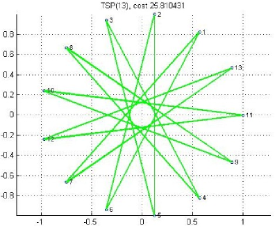
Figure 30: POME₁₃ is a star.

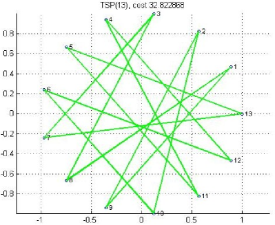
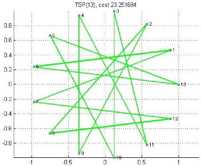
a) b)

Figure 31: a) POMa₁₃ is no star, and b) POMm₁₃ is no star.

Figure 32: POME₁₄ is no star.

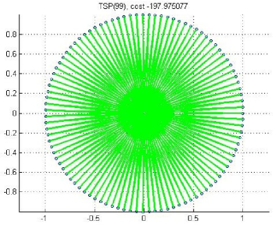
Figure 33: POME₉₉ is a star.

As in previous sections, the study of a problem allow to discover properties for building efficient algorithm. The convexity and an appropriate lattices for Lennard-Jones problems (LJP_n) are important properties used in [9, 10]. However, these properties can not be generalized or inherited to other NP problems.

8 There is not a property for solving GAP

The algorithm 1 is blind to the properties of TSP and KTP. Jordan’s simple curve and hamiltonian cycles with many cross as posible are clearly oppositive properties.

For KTP, the objective function is adapted for solving a decision problem: is there a hamiltonian cycle for a knight in a chessboard $8\times 8$?

The rippling effects proves that GAP’s the objective function giving by the summation os the edges’ cost is not monotonic or convex. This can see assuming few $c_{ij}>0$ and their corresponding $c_{ij}<0$.

Proposition 8.1.

Given a GAP_n there is $\mathbb{R}^{K}$ where the vertices of GAP can be located as points in $\mathbb{R}^{K}$ with the max distance $d_{m}$.

Proof.

The unknowns are the coordinates of each vertex. Linear equations can be generated from the edge’s cost.

Without loss of generality, I assume that the cost matrix is asymmetrical. For $K>0,L_{j}\leq K$, the linear system to solve is:

$$x^{1}_{1}-x^{2}_{1}+x^{1}_{2}-x^{2}_{2}+\cdots+x^{1}_{K-1}-x^{2}_{K-L_{1}}+x^{1}_{K-L_{1}+1}+\cdots+x^{1}_{K} = c_{1,2}$$

$$x^{1}_{1}-x^{2}_{1}+x^{1}_{2}-x^{2}_{2}+\cdots+x^{1}_{K-1}-x^{2}_{K-L_{2}}-x^{2}_{K-L_{2}+1}+\cdots-x^{2}_{K} = c_{2,1}$$

$$\vdots = \vdots,$$

$$x^{n}_{1}-x^{n-1}_{1}+x^{n}_{2}-x^{n-1}_{2}+\cdots+x^{n}_{K-L_{n^{2}-1}}-x^{n-1}_{K-L_{n^{2}-1}}+x^{n-1}_{K-L{n^{2}-1}+1}+\cdots+x^{n-1}_{K} = c_{n-1,n},$$

$$x^{n}_{1}-x^{n-1}_{1}+x^{n}_{2}-x^{n-1}_{2}+\cdots+x^{n}_{K-L_{n^{2}}}-x^{n-1}_{K-L_{n^{2}}}-x^{n}_{K-L{n^{2}}+1}-\cdots-x^{n}_{K} = c_{n,n-1},$$

where $x^{i}=(x^{i}_{1},x^{i}_{2},\ldots,x^{i}_{K})$ $\in$ $\mathbb{R}^{k},$ $i=1,\ldots,n$ are the corresponding coordinates of the vertices. With sufficient variables, i.e, appropriate values of $K$ and $L_{j}$, $j=1,2,\ldots,n^{2},$ the previous linear system is always soluble. ∎

Remark 8.2.

Any GAP can be mapped in $\mathbb{R}^{K}$ under $d_{m}$.

In the core of the algorithms for TSP and KTP is the algorithm 1. It is designed for exploring edges’cost for looking a minimum or for doing a random uniform search. The heuristic used in the algorithm for TSP is well know, but it only works for a plane where the distance fulfil the cosine law of the triangles, i.e., where Prop. 6.11 in  [10] holds. Even, in 3D TSP does not comply. Figure 27 depicts an initial hamiltonian cycle for a TSP with 40 cities in a 3D Space with cost = $29.2243$. Figure 28 depicts a putative optimal hamiltonian cycle with cost = $23.6998$. There is a reduction on the cost, but, both figures b) imply that there are many alternatives to explore yet.

On the other hand, KTP could be solved requiring hamiltonian cycles with length equals to $n\times m\times 5$ with $dist(x,y)$ $=$ $\left(i-i^{\prime}\right)^{2}+\left(j-j^{\prime}\right)^{2}$, where $x=(i,j),$ and $y=(i^{\prime},j^{\prime}),$ $1\leq i,i^{\prime}\leq n$, and $1\leq j,j^{\prime}\leq m$. In this case the objective function could used without changes, but algorithm 1 must be modified to random uniform search (see  3.1).

9 SAT_n×m has not properties for an efficient algorithm

This section is devoted to a former NP problem. I apply my technique: 1) general problem, 2) simple reduction, and 3) there is no property for building an efficient algorithm for the simple reduction problem.

Here, I use the convention to represent $\overline{x_{i}}$ to $0$ (false), $x_{i}$ to $1$ ( true), and 2 when the variable $x_{i}$ is no present. Let $\Sigma=\left\{0,1\right\},$ $x_{i}:\Sigma\rightarrow\Sigma,x_{i}\left(v\right)=v,v\in\Sigma,\overline{x}_{i}:\Sigma\rightarrow\Sigma,\overline{x}_{i}\left(v\right)=\rceil v,v\in\Sigma$ (logical not).

A particular Boolean Satisfiability Problem (SAT) consists in finding a set of values in $\Sigma$ of $n$ bolean variables and $m$ formulas to have the following system equal to 1:

$$\begin{array}[]{l}\ \ (x_{1}\vee\overline{x_{2}}\vee\cdots\vee x_{l}\cdots\vee x_{n})\\ \wedge(x_{1}\vee x_{2}\vee\cdots\vee x_{n-1})\\ \vdots\\ \wedge(\overline{x_{2}}\vee x_{3}\vee\cdots\vee\overline{x_{i}}\cdots\vee x_{l}).\end{array}$$

Then the general problem or complex SAT is where the formulas could have any subset of boolean variables, where each formula can be mapped to a ternary number.

For example:

$$\begin{array}[]{l}\ \ (x_{5}\vee\overline{x_{4}}\vee x_{1})\\ \wedge(x_{3}\vee x_{2})\\ \wedge(\overline{x_{4}}\vee x_{3}\vee\overline{x_{2}}\vee x_{1}).\end{array}$$

It is traduced to:

$$\begin{array}[]{l}10221\\ 22112\\ 20101.\end{array}$$

The assignment $x_{1}=1$, $x_{2}=1$ satisfies the previous example. It is not unique. Moreover, the number 22211 is a representation of this assignment as a ternary number. Also, the system:

$$\begin{array}[]{l}\ \ (x_{5}\vee\overline{x_{4}}\vee x_{1})\\ \wedge(x_{3}\vee x_{2})\\ \wedge(\overline{x_{4}}\vee x_{3}\vee\overline{x_{2}}\vee x_{1})\\ \wedge(x_{2}\vee x_{1}).\end{array}$$

22211 is translated like the last formula and it is a type of a fixed point system, where 22211 is an appropriate assignment. The details are given below.

On the other hand, the simple reduction provides a simple version of SAT, where for convenience all formulas have the same variables. In any case, this simple versión of SAT is like study parts of the complex SAT, and it is sufficient to prove that there is not polynomial time algorithm for the simple SAT, and also, for general SAT.

An equivalent functional formulation is:

Let $\overrightarrow{x}=\left(x_{1,}x_{2},\ldots,x_{n}\right)\in\Sigma^{n},\overrightarrow{y}\in\Sigma^{m},S_{j}\subset\{1,\ldots,n,-1,\ldots,-n\},j=1,\ldots,m,$ $F_{j}:\Sigma^{m}\rightarrow\Sigma,F_{j}\left(\overrightarrow{x}\right)=\vee_{k\in S_{j}}z_{k},z_{k}=\left\{\begin{array}[]{cc}x_{k}&k>0\\ \overline{x}_{k}&k<0\end{array}\right.,$ $G:\Sigma^{m}\rightarrow\Sigma,G\left(\overrightarrow{y}\right)=\wedge_{i=1}^{m}y_{i}$

The SAT is

$$G\circ\left(F_{1},\ldots,F_{m}\right)\left(\overrightarrow{x}\right).$$

Let be U$=[u_{jk}]$ a matrix of $\Sigma^{m\times 2n},$

$u_{j,k}=\left\{\begin{array}[]{cc}1&\text{if }x_{i}\vee\overline{x}_{i}\text{ are variables of }F_{j},k=i,\text{if }i>0,k=n+|i|,\text{if }i<0,\\ 0&\text{otherwise.}\end{array}\right.$

The matrix U let to know how many variables has $F_{j}$ as the of summation over the row, $\sum_{i=1}^{2n}(u_{ji})$. Also the summation over a column, $\sum_{j=1}^{m}(u_{jk})$ is the number of times that the $x_{i}$ or $\overline{x}_{i}$ ($k=i,\text{if }i>0,\text{ or }k=n+|i|,\text{if }i<0$) is used in all $F_{j}$.

Let be $\blacksquare$ as 0, and $\square$ as 1. The following boards have not a set of values in $\Sigma$ to satisface them (I called unsatisfactory boards):

$$x_{1}$$

      

Hereafter, a SAT of $n$ bolean variables and $m$ formulas is denoted by SAT$n\times m$.

Proposition 9.1.

Given a SAT_n×2n where formulas as the squares correspond to the $0$ to $2^{l}-1$ binary values, is an unsatisfactory board.

Proof.

The binary values from $0$ to $2^{l}-1$ are all posibles assignation of values for the board. It means that for any possible assignation, there is the oppositive formula with value 0. ∎

Proposition 9.2.

Given a SAT of $n\times m$, there is not a satisfactory set of values in $\Sigma$, when there is a subset of $l$ bolean variables and their set of $Fj$ formulas are isomorphic to an unsatisfactory board.

Proof.

It is immediately, the subset of $l$ bolean variables can not satisface their $2^{l}$, $F_{j}$ formulas. Therefore, there is not posible to find satisfactory set of $n$ values for this SAT. ∎

When I focusses in the classical techniques for fixed point or finding roots. The formulation of one can be used in the other. This means $f:\mathbb{R}\rightarrow\mathbb{R}$ with a root $x_{1}^{\ast}$ $\in$ $(a,b)$ then the function $g:\mathbb{R}\rightarrow\mathbb{R}$, giving by $g(x)=x+f(x)$ has the fixed point $x_{1}^{\ast}$. The reciprocal, let the function $g:\mathbb{R}\rightarrow\mathbb{R}$ has a fixed point $x^{\ast}$ then the function $f:\mathbb{R}\rightarrow\mathbb{R}$, giving by $f(x)=x-g(x)$ has the point $x_{1}^{\ast}$ as a root.

SAT_n×m can be transformed in a fixed point formulation. This formulation is easy to understand, it consists in:

1. $\Sigma=\{0,1\}$.

2. giving a boolean variable $x$ is mapped to 1, and $\overline{x}$ to 0;

3. a formula: $\overline{x_{n-1}}\vee\cdots x_{l}\vee\cdots\vee\overline{x_{1}}\vee x_{0}$ can be transformed in its corresponding binary number: $0\cdots 1\cdots 01$;

4. if a $y$ is a binary number, $\overline{y}$ is the complement binary number. this is done bit a bit, 0 is complemented to 1 and 1 is complemented to 0.

5. a system of SAT_n×m correspond the set $M_{n\times m}$ of the $m$ binary numbers of its formulas. $M_{n\times m}=\{\begin{array}[]{c}s_{n-1}^{1}s_{n-2}^{1}\cdots s_{1}^{1}s_{0}^{1},\\ s_{n-1}^{2}s_{n-2}^{2}\cdots s_{1}^{2}s_{0}^{2},\\ \ldots,\\ s_{n-1}^{m}s_{n-2}^{m}\cdots s_{1}^{m}s_{0}^{m}\end{array}\}.$ Note that the number $s_{n-}^{k}s_{n-2}^{k}\cdots s_{1}^{k}s_{0}^{k}$ correspond to formula $k$ of the SAT_n×m, $k=1,\ldots,m$.

6. a system of SAT_n×m as a boolean function is SAT${}_{n\times m}:\Sigma^{n}\rightarrow\Sigma$. The argument is a binary number of n bits.

Proposition 9.3.

Evaluation of SAT_n×m is equivalent to the evaluation of SAT${}_{n\times m}(y=y_{n-1}y_{n-2}\cdots y_{1}y_{0})$, that consists to verify $y_{i}$ match a digit $s_{i}^{k}\in M_{n\times m},$ $\forall k=1,\ldots,m$, SAT${}_{n\times m}(y=y_{n-1}y_{n-2}\cdots y_{1}y_{0})$=1, otherwise SAT${}_{n\times m}(y=y_{n-1}y_{n-2}\cdots y_{1}y_{0})$=0.

Proof.

It is immediately, let $x_{i}=v_{i}$, $i=n,\ldots,1$ with $v_{i}\in\Sigma$ an assignation for SAT_n×m. If the set of values $v_{i}$ satisfies SAT_n×m then it means that at least one bolean variable of each bolean formula is 1, therefore SAT$n\times m(v_{n}v_{n-1}\cdots v_{2}v_{1})$ is 1. By other hand, if $x_{i}=v_{i}$ does not satisfice SAT_n×m, then at least one formula the SAT_n×m is 0, let assume it is j. This means that no value $v_{i}$ match any digit of $s^{j}_{i}$ for $i=n,\ldots,1$. Therefore SAT${}_{n\times m}(v_{n}v_{n-1}\cdots v_{2}v_{1})=0.$

Reciprocally, SAT${}_{n\times m}(y=y_{n}y_{n-1}\cdots y_{2}y_{1})=1$, means that a digit $y_{i}$ match a digit $s_{i}^{k}\in M,$ $\forall k=1,\ldots,m.$ The k bolean formulas are 1. Therefore, SAT_n×m is 1 with the assignation $x_{i}=y_{i}.$ Otherwise,SAT${}_{n\times m}(y=y_{n}y_{n-1}\cdots y_{2}y_{1})=0$ implies that at least one binary number of $M$ does not coincide with the digits of $y$. This means a bolean formula of SAT_n×m is 0, then SAT_n×m is 0. ∎

Proposition 9.4.

An equivalent formulation of SAT_n×m is to look for a binary number $x^{\ast}$ from $0$ to $2^{n}-1.$

1. $x^{\ast}\in M_{n\times m}$ and $\overline{x^{\ast}}\notin M_{n\times m}$ then SAT${}_{n\times m}(x^{\ast})=1.$

2. $x^{\ast}\in M_{n\times m}$ and $\overline{x^{\ast}}\in M_{n\times m}$ then SAT${}_{n\times m}(x^{\ast})=0.$ If $m<2^{n}-1$ then $\exists y^{\ast},0\leq y^{\ast}\leq 2^{n}-1$ with $\overline{y^{\ast}}\notin M_{n\times m}$ and SAT${}_{n\times m}(y^{\ast})=1.$

Proof.

1. How $x^{\ast}\in M_{n\times m}$ and $\overline{x^{\ast}}\notin M_{n\times m}$, this means that the corresponding formula of $x^{\ast}$ is not blocked and for each bolean formula of SAT${}_{n\times m}(x^{\ast})$ at least one bolean variable coincides with one variable of $x^{\ast}.$ Therefore SAT${}_{n\times m}(x^{\ast})=1.$

2. How $m<2^{n}-1$, $\exists y^{\ast},0\leq y^{\ast}\leq 2^{n}-1$ with $\overline{y^{\ast}}\notin M_{n\times m}.$ Adding the corresponding formula of $y^{\ast}$ to SAT_n×m, a new SAT_n×m+1 is obtained. By the previous case, the case is proved.

∎

This approach is quite forward to verify and get a solution for any SAT_n×m. By example given SAT_6×4, its correspond set $M_{6\times 4}$:

$$\begin{tabular}[]{|l|l|l|l|l|l|l|}\hline\cr&$x_{5}=0$&$x_{4}=0$&$x_{3}=0$&$x_{2}=0$&$x_{1}=0$&$x_{0}=0$\\ \hline\cr&$\overline{x_{5}}\vee$&$\overline{x_{4}}\vee$&$\overline{x_{3}}\vee$&$\overline{x_{2}}\vee$&$\overline{x_{1}}\vee$&$\overline{x_{0}})$\\ \hline\cr$\wedge($&$\overline{x_{5}}\vee$&$\overline{x_{4}}\vee$&$\overline{x_{3}}\vee$&$\overline{x_{2}}\vee$&$\overline{x_{1}}\vee$&$x_{0})$\\ \hline\cr$\wedge($&$x_{5}\vee$&$x_{4}\vee$&$x_{3}\vee$&$x_{2}\vee$&$x_{1}\vee$&$\overline{x_{0}})$\\ \hline\cr$\wedge($&$\overline{x_{5}}\vee$&$x_{4}\vee$&$x_{3}\vee$&$\overline{x_{2}}\vee$&$x_{1}\vee$&$x_{0})$\\ \hline\cr\end{tabular}\text{ \ }\begin{array}[]{c}\\ \left[\overline{x_{0}}\right]\equiv 1\\ \left[\overline{x_{1}}\right]\equiv 1\\ \left[\overline{x_{0}}\right]\equiv 1\\ \left[\overline{x_{2}}\right]\equiv 1\end{array}\text{ \ }\begin{tabular}[]{|l|l|l|l|l|l|}\hline\cr$x_{5}$&$x_{4}$&$x_{3}$&$x_{2}$&$x_{1}$&$x_{0}$\\ \hline\cr$0$&$0$&$0$&$0$&$0$&$0$\\ \hline\cr$0$&$0$&$0$&$0$&$0$&$1$\\ \hline\cr$1$&$1$&$1$&$1$&$1$&$0$\\ \hline\cr$0$&$1$&$1$&$0$&$1$&$1$\\ \hline\cr\end{tabular}\text{.}$$

The left side depicts that SAT${}_{6\times 4}(y=000000)=1$. The right side depicts the set $M_{6\times 4}$ as an array of binary numbers , where $000000\in M_{6\times 4}.$ The middle column depicts at least one variable that satisfies the boolean formulas of SAT${}_{6\times 4}.$ Also, $y$ $=$ $000000$ can be interpreted as the satisfied assignment $x_{5}=0,$ $x_{4}=0,$ $x_{3}=0,$ $x_{2}=0,$ $x_{1}=0,$ and $x_{0}=0.$

In fact, the previous proposition gives an interpretation of the SAT as a type fixed point problem.

Proposition 9.5.

Given a SAT_n×m, there is a binary number $y\in M_{n\times m}$ such that $\overline{y}\notin M_{n\times m}$ then $y$ is fixed point for SAT_n×m or SAT${}_{n\times m+1}(y)$, where SAT_n×m+1 is SAT_n×m with adding the corresponding formula of $y$ to SAT${}_{n\times m}.$

Proof.

This result follows from the previous proposition. ∎

Using the propositions and properties for SAT${}_{n\times m},$ a computable algorithm for solving SAT_n×m is:

Algorithm 6.

Input: SAT_n×m.

Output: $x^{\ast}$ such that SAT${}_{n\times m}(x^{\ast})=1$ or SAT${}_{n\times m+1}(x^{\ast})=1$ or SAT_n×m is not satisfied.

Variables in memory: T[0:$2^{n-1}$]=0 of boolean. $mi$:=$2^{n}$ : Integer, $mx$:=-1: Integer; $ct$:=0 : Integer;

1. for i:=1 to m

2. Translate formula $i$ of SAT_n×m to a binary number $k$.

3. if T[$k$] not equal 1 then

4. if SAT_n×m($k$) equal 1 then

5. output: $k$ is the solution for SAT_n×m.

6. stop

7. end if

8. T[$k$] := 1;

9. $ct$ := $ct$ + 1;

10. $mi$ := Min($k$,$mi$);

11. $mx$ := Max($k$, $mx$);

12. end if

13. end for

14. if mi == 0 and mx == $2^{n-1}$ and ct $\geq$ $2^{n}$ then

15. output: There is not solution for SAT_n×m.

16. stop

17. end if

18. if $mi$ $>$ $1$ and SAT_n×m($mi-1$) == 1 then

19. output: $mi-1$ is the solution for SAT_n×m+1 with the corresponding formula for $mi-1$.

20. stop

21. end if

22. if mx $<$ $2^{n}-1$ and SAT_n×m($mx+1$) == 1 then

23. output: $mx+1$ is the solution for SAT_n×m+1 with the corresponding formula for $mx+1$.

24. stop

25. end if

26. for i:=0 to $2^{n}-1$

27. if T[$i$] not equal 1 then

28. output: $i$ is the solution for SAT_n×m+1 with the corresponding formula for $i$.

29. stop

30. end if

31. end for

At this point, SAT_n×m is equivalent to set of binary numbers M_n×m. The knowledge for a given SAT_n×m depends at least from exploring M_n×m. Before of exploring SAT_n×m no binary numbers associated with it are know. Now, let $\mathbb{K}_{n\times m}$ be knowledge of a given SAT_n×m. $\mathbb{K}_{n\times m}$ $=$ $\left\{y^{\ast}\right\}$ $\cup$ M_n×m $\cup$ $\mathbb{S}_{n\times m}$, where $y^{\ast}$ is the satisfying number for SAT_n×m, and $\mathbb{S}_{n\times m}$ $=$ M${}_{n\times m}^{c}$, it is the set of binary numbers that satisfies SAT_n×m. Using the previous proposition, without lost of generality, $y^{\ast}\in$ M_n×m.

Proposition 9.6.

Given a SAT_n×m, and $\mathbb{K}_{n\times m}$:

1. It is trivial to solve SAT${}_{n\times m}.$

2. It is trivial to solve SAT_n×m+1 from M_n×m $\cup$ $\{\overline{y}^{\ast}\}$.

Proof.

1. $y^{\ast}$ solves SAT${}_{n\times m}.$

2. Any $s\in\mathbb{S}_{n\times m}\setminus\{\overline{y}^{\ast}\}$ solves SAT_n×m+1.

∎

The previous proposition depicts the condition needed to solve efficiently SAT_n×m, which is $\mathbb{K}_{n\times m}$ the knowledge associated with the specific given SAT_n×m.

It is not complicate and complex to create an object data structure combined index array and double links, the drawback is the amount of memory needed to do the insertion and erase with cost $\mathbf{O}(k)$ ($k$ very small integer) by updating only the links.

Assuming that the initial states of the structures for $\mathbb{S}$ and M are giving, it cost for building them can be neglected or considered a constant. Of course the amount of memory needed is exponential $(2^{n}),$ where $n$ is the numbers of boolean variables for SAT_n×m

The next tables depict that inserting and erasing binary numbers into the structures $\mathbb{S}$ and M only consists on updating links with fixed complexity $\mathbf{O}(k)$ ($k$ very small integer comparing with $2^{n}$).

Est prev next $\mathbb{S}$ 8 1 M 0 0    $\mathbb{S}_{n\times m}$ $i$ $n$ prev_i next_i 1 000 8 2 2 001 1 3 3 010 2 5 4 011 0 0 5 100 3 6 6 101 5 7 7 110 6 8 8 111 7 1    M_n×m $i$ $n$ prev_i next_i 1 - - - 0 0 2 - - - 0 0 3 - - - 0 0 4 - - - 0 0 5 - - - 0 0 6 - - - 0 0 7 - - - 0 0 8 - - - 0 0

Erasing $011$ from $\mathbb{S}_{n\times m}$ and inserting it in M_n×m

Est prev next $\mathbb{S}$ 8 1 M 4 4    $\mathbb{S}_{n\times m}$ $i$ $n$ prev_i next_i 1 000 8 2 2 001 1 3 3 010 2 5 4 - - - 0 0 5 100 3 6 6 101 5 7 7 110 6 8 8 111 7 1    M_n×m $i$ $n$ prev_i next_i 1 - - - 0 0 2 - - - 0 0 3 - - - 0 0 4 011 4 4 5 - - - 0 0 6 - - - 0 0 7 - - - 0 0 8 - - - 0 0

Erasing $001$ from $\mathbb{S}_{n\times m}$ and inserting it in M_n×m

Est prev next $\mathbb{S}$ 8 1 M 4 2    $\mathbb{S}_{n\times m}$ $i$ $n$ prev_i next_i 1 000 8 3 2 - - - 0 0 3 010 1 5 4 - - - 0 0 5 100 3 6 6 101 5 7 7 110 6 8 8 111 7 1    M_n×m $i$ $n$ prev_i next_i 1 - - - 0 0 2 001 4 4 3 - - - 0 0 4 011 2 2 5 - - - 0 0 6 - - - 0 0 7 - - - 0 0 8 - - - 0 0

Erasing $000$ from $\mathbb{S}_{n\times m}$ and inserting it in M_n×m

Est prev next $\mathbb{S}$ 8 3 M 4 1    $\mathbb{S}_{n\times m}$ $i$ $n$ prev_i next_i 1 - - - 0 0 2 - - - 0 0 3 010 8 5 4 - - - 0 0 5 100 3 6 6 101 5 7 7 110 6 8 8 111 7 3    M_n×m $i$ $n$ prev_i next_i 1 000 4 2 2 001 1 4 3 - - - 0 0 4 011 2 1 5 - - - 0 0 6 - - - 0 0 7 - - - 0 0 8 - - - 0 0

Using the structures, propositions and properties for SAT${}_{n\times m},$ a computable algorithm for solving SAT_n×m and building $\mathbb{K}_{n\times m}$ is:

Algorithm 7.

Input: SAT_n×m.

Output: Y set of binary numbers, such that when Y$\neq\{\},$ any $y\ast\in$ Y, SAT${}_{n\times m}(y^{\ast})=1$. The structure $\mathbb{S}_{n\times m}$, such that any $x^{\ast}\in\mathbb{S}_{n\times m}$, SAT${}_{n\times m+1}(x^{\ast})=1$. $\mathbb{K}_{n\times m}$ (object structures: M, $\mathbb{S}_{n\times m}$ and Y).

Variables in memory: Y $=\{\}$: set of binary numbers, initialized to empty; Initialized object structures: M, $\mathbb{S}_{n\times m}$.

1. for i:=1 to m

2. Translate formula $i$ of SAT_n×m to a binary number $k$.

3. if $\mathbb{S}$.$\mathbb{S}_{n\times m}$[$k$] not equal ”- - -” then

4. if SAT_n×m($k$) equal 1 then

5. output: $y^{\ast}=k$ is a solution for SAT_n×m.

6. insert($k$, Y).

7. $\textbf{delete}(k,\mathbb{S}_{n\times m})$

8. $\textbf{insert}(k,\text{M}_{n\times m})$

9. else

10. $\textbf{delete}(k,\mathbb{S}_{n\times m})$

11. $\textbf{insert}(k,\text{M}_{n\times m})$

12. $\textbf{delete}(\overline{k},\mathbb{S}_{n\times m})$

13. $\textbf{insert}(\overline{k},\text{M}_{n\times m})$

14. end if

15. end if

16. end for

At this point, SAT_n×m is equivalent to set of binary numbers M_n×m. And $\mathbb{K}_{n\times m}$ has information to solve SAT_n×m immediately.

The knowledge for a given SAT_n×m depends of exploring M_n×m. Before of exploring SAT_n×m no binary numbers associated with $\mathbb{K}_{n\times m}$.

Now, let $\mathbb{K}_{n\times m}$ be knowledge of SAT_n×m. $\mathbb{K}_{n\times m}$ $=$ Y $\cup$ M_n×m $\cup$ $\mathbb{S}_{n\times m}$, where Y is the set of satisfying number for SAT_n×m, and $\mathbb{S}_{n\times m}$ $=$ (Y $\cup$ M${}_{n\times m})^{c}$, it is the set of binary numbers that satisfies SAT_n×m.

Remark 8.

Having $\mathbb{K}_{n\times m}$, the knowledge of SAT_n×m, it is easy to solve any modified SAT_n×m. It is need to keep tracking of changes in M and $\mathbb{S}$, then modified SAT can be solved by the proposition 9.6.

So far, SAT_n×m is now a fixed point type problem over a set of binary numbers. It consists in look for a number in M_n×m which is not blocked or to pick up any element $s$ $\in\mathbb{S}_{n\times m}$ when $\mathbb{K}$ is given.

If all number of M_n×m are blocked then the first binary number $s$ from 0 to $2^{n}-1$ which is not in M_n×m is the solution for M_n×m, i.e. any element $s$ $\in\mathbb{S}_{n\times m}$. This is trivial when knowledge is given or can be created in an efficient way. This results of this section are related to my article  [10], where I stated that NP problems need to look for its solution in an search space using a Turing Machine: ”It is a TM the appropriate computational model for a simple algorithm to explore at full the GAPn s research space or a reduced research space of it”. As trivial as it sound, pickup a solution for SAT_n×m depends of exploring its $m$ boolean equations.

The question if there exists an efficient algorithm for any SAT_n×m now can be answered. The algorithm 7 is technologically implausible because the amount of memory needed. However, building $\mathbb{K}_{n\times m}$ provides a very efficient telephone algorithm (see proposition 8, and remarks 5 in [9]) where succeed is guaranteed for any $s$ $\in$ $\mathbb{S}_{n\times m}$. On the other hands, following  [9]) there are tree possibilities exhaustive algorithm (exploring all the searching space), scout algorithm (previous knowledge or heuristic facilities the search in the searching space), and wizard algorithm (using necessary and sufficient properties of the problem).

The study of NP problems depicts that only for an special type of problem exists properties such as Jordan’s simple curve or $n$ odd for polygon for TSP2D, or convexity, IF lattice, or CB lattice for Lennard Jones structural and potential minimization problems for building an ad-hoc efficient algorithms, but these properties can not be generalizad for any GAP or any member of class NP.

The boolean formulas of SAT_n×m correspond a binary numbers in disorder (assuming an order of the boolean variables as binary digits). The algorithm 6 has a complexity of the size of $m$ (the numbers of formulas of SAT).It is not worth to considered sorting algorithm because complexity increase by a factor $\mathbf{O}(n(2^{n}))$ when $m\approx 2^{n}.$

Without exploring, given SAT_n×m then build M_n×m. M can be consider an arbitrary set of numbers. The numbers in M have not relation or property to point out the satisfied binary number, in fact one or many numbers could be solution or not one in M, but in the range from 0 to $2^{n}-1$ there is a solution or not depending of M. Of course, this is true for an arbitrary set of numbers.

On the other hand, if the formulas of a SAT problem are formulated assuming, by example, no boolean formula is complement of other one, then any translation to binary number is a satisfied assignment.

Hereafter, for the sake of my argumentation the boolean formulas of SAT_n×m are considered a translation to binary numbers in disorder and without any correlation in M_n×m.

Proposition 9.7.

With algorithm 6:

1. A solution for SAT_n×m is efficient when $m<<$ $2^{n}.$

2. A solution for SAT_n×m is not efficient when $m\approx$ $2^{n}.$

Proof.

It follows from algorithm 6. ∎

In order to find a solution for SAT, there are a probabilistic algorithm rather than algorithm 6. By example a simple probabilistic algorithm for SAT_n×m is:

Algorithm 9.

Input: SAT_n×m.

Output: $x^{\ast}$ such that SAT${}_{n\times m}(x^{\ast})=1$ or SAT${}_{n\times m+1}(x^{\ast})=1$ or SAT_n×m is not satisfied.

Variables in memory: T[0:$2^{n-1}$]=0 of boolean. $ct$:=0 : Integer;

1. while (1)

2. Select randomly $k$ in $[0,2^{n}-1]$ minus marked T[i]==1;

3. if SAT_n×m($k$) == 1 then

4. output: $k$ is the solution for SAT_n×m.

5. stop

6. end if

7. if T[$k$] $<>1$ then

8. T[$k$]:=1;

9. $ct$ := $ct$ +1;

10. if $ct\geq 2^{n}$ then

11. output: There is not solution for SAT_n×m.

12. stop

13. end if

14. end while

Proposition 9.8.

With algorithm 9:

1. A solution for SAT_n×m is efficient when $m<<$ $2^{n}.$

2. A solution for SAT_n×m is not efficient when $m\approx$ $2^{n}.$

Proof.

1. It follows from algorithm 9 for finding $k$ and $m<<$ $2^{n}$. It implies, for many $k$ that P(SAT_n×m($k$)==1) $\approx 1$.

2. It follows from algorithm 9 for finding $k$ and $m\approx$ $2^{n}$. Here, it is possible that many selected randomly number in $[0,2^{n}-1]$ are blocked. Therefore P(SAT_n×m($k$)==0) $\approx 1$. This could cause that algorithm 9 does not solve SAT_n×m in an appropriate amount of time.

∎

Finally,

Proposition 9.9.

SAT_n×m has not property or heuristic to build an efficient algorithm.

Proof.

Given SAT_n×m, its translation is a set of binary numbers, in disorder and without any any previous knowledge, nor correlation in M_n×m. If such property or heuristic exist then any arbitrary subset of number has it. Such characteristic or property must imply that any natural number is related to each other. This means it is in the intersection of all properties for all natural numbers. Also it is no related to the value, because by example, the intersection of natural clases under the modulo of a prime number is empty. Moreover, it is something a priory, otherwise, it will imply to revise all number at least in M_n×m. Using it in a random algorithm, to point out efficiently to the number, which is solution, means that this number is inherently not equally probable. Also, this binary number correspond to an arbitrary arrangement of the boolean variables of SAT_n×m, so in a different arrangement of the positions for the boolean variables, any number is inherently not equally probable! ∎

Proposition 9.10.

NP has not property or heuristic to build an efficient algorithm.

Proof.

Let be X a problem in NP. PH${{}_{\text{X}}}$ is the set of properties or heuristics for building an efficient algorithm for problem X.

$$\bigcap_{\text{X}}\text{PH}{{}_{\text{X}}}=\{\}$$

by the previous proposition. ∎

Conclusions and future work

The Jordan’s simple curve is an example of a property to create an efficient algorithm for a necessary type of solution of a NP hard problem. It is for solving approximately Euclidian Travelling Salesman problem in 2D planes but not in $\mathbb{R}^{m}$ spaces, $m>2$. Here the Euclidian metric implies that the quadrilateral’sides are less than the quadrilateral’s diagonals. Polygon or convex distribution of the cities, Jordan is a sufficient and necessary property, this previous knowledge allows to build efficient algorithms. For $\mathbb{R}^{m}$, even with fast triangulations, this means more alternatives to explore, without a property to reduce global complexity in the corresponding searching space.

Heuristic techniques, using previous knowledge of a problem in $\mathbb{R}^{m}$ do not provide reducibility (see 6 in  [10]) for any NP problems.

There are nice properties Jordan’s simple curve and star. Any POME_n, $n>3$ odd has a solution type star. Any TSP2D has a solution as a Jordan’s simple curve. Crossing lines in a solution is the opposite of not crossing lines in other type of problem.

For LJ problems or for the Searching of the Optimal Geometrical Structures of clusters of $n$ particles remains out of the existence of an efficient algorithm, the selection of the $n$ particles is the bottle’s neck (see  [9]).

Here, the classical SAT (a NP decision problem) provides a general case, where formulas have any number of boolean variables, then it is is reduced to a simple version SAT${n\times m}$, all boolean formulas have the same number of boolean variables. This allows to see that does not exist a property for solving SAT with reducibility of the searching space. This shows that there is not a general property that allows to solve SAT problems in polynomial time. The classical SAT depicted in section 9 has clearly no properties for solving efficiently it when $m\approx 2^{n}$.

For the future, I believe that the implementation of the algorithm 2 for TSP brings an efficient time’s reduction for finding the optimal hamiltonian cycle under euclidian distance versus looking to solve a global optimization problem without a necessary stop condition.

Quantum Computation is on the future road. To my knowledge the algorithm 6 can be adapted for using quantum variables for exploring $[0,2^{n}-1]$ states at the same time, instead of the cycle for i:=0 to $2^{n}-1$. This implies that the complexity for solving NP problems can be reduced to one cycle over quantum variables.

Finally, this reformulation of my previous works, using Jordan’s simple curve versus hamiltonian cycles with many crossings as possible, and the research of the properties of SAT_n×m supports that there is not a general property to reduce the complexity of the worst case NP problem.

References

- [1] Concorde Home. Concorde TSP Solver. Department of Mathematics of the University of Waterlo. http://www.math.uwaterloo.ca/tsp/concorde.html, 2011.
- [2] A. Aggoun, N. Beldiceanu, E. Bourreau, and H. Simonis. Generalised Euler’s knight. http://4c.ucc.ie/ hsimonis/Generalised Eulers Knight.pdf, 2008.
- [3] N. Amenta, D. Attali, and O. Devillers. Complexity of delaunay triangulation for points on lower-dimensional polyhedra. In SODA ’07: Proceedings of the eighteenth annual ACM-SIAM symposium on Discrete algorithms, pages 1106–1113, Philadelphia, PA, USA, 2007. SIAM.
- [4] D. L. Applegate, R. E. Bixby, V. Chvatal, and W. J. Cook. The Traveling Salesman Problem: A Computational Study (Princeton Series in Applied Mathematics). Princeton University Press, Princeton, NJ, USA, 2007.
- [5] C. Barrón. Manual de referencia de los programas de los métodos de tunelización: Clásico y Exponencial. Technical Report Manual 2, IIMAS-UNAM, Noviembre de 199 1991.
- [6] C. Barrón, S. Gómez, and D. Romero. Archimedean Polyhedron Structure Yields a Lower Energy Atomic Cluster. Applied Mathematics Letters, 9(5):75–78, 1996.
- [7] C. Barrón, S. Gómez, D. Romero, and A. Saavedra. A Genetic Algorithm for Lennard-Jones Atomic clusters. Applied Mathematics Letters, 12:85–90, 1999.
- [8] C. Barrón-Romero. Propuesta. Tema: Optimización discreta. http://ce.azc.uam.mx/profesores/cbr/PDF/ProyectoTerminal 2013.pdf.
- [9] C. Barrón-Romero. Minimum search space and efficient methods for structural cluster optimization. ArXiv, pages Math–ph:0504030 v4, 2005.
- [10] C. Barron-Romero. The complexity of the np-class. arXiv.org, abs/1006.2218, 2010.
- [11] C. Barron-Romero. The complexity of euclidian 2 dimension travelling salesman problem versus general assign problem, NP is not P. arXiv.org, abs/1101.0160, 2011.
- [12] C. Barrón-Romero. Conjugate Gradient Algorithm for Solving a Optimal Multiply Control Problem on a System of Partial Differential Equations. ArXiv e-prints, Mar. 2014.
- [13] R. Borndörfer, M. Grötschel, and A. Löble. Mathematics Everywhere, chapter 4. The Quickest Path to the Goal. Spain - AMS, 2010.
- [14] R. Chingizovich Valeyev. ”P = NP” versus ”P NP”. Life Science Journal, 11(12s):506–512, Personal Comunication 2014.
- [15] R. Glowinski. Numerical Methods for Nonlinear Variational Problems. Computational Physics. Springer-Verlag, 1984.
- [16] S. Gómez and C. Barrón. The Exponential Tunneling Method. Technical Report Research Report 3(1), IIMAS-UNAM, Julio 1991 1991.
- [17] S. Gómez, J. Solano, L. Castellanos, and M. I. Quintana. Tunneling and genetic algorithms for global optimization. In N. Hadjisavvas and P. Pardalos, editors, Advances in Convex Analysis and Global Optimization, volume 54 of Nonconvex Optimization and Its Applications, pages 553–567. Springer US, 2001.
- [18] G. J Woeginger. The P-versus-NP page. http://www.win.tue.nl/ gwoegi/P-versus-NP.htm.
- [19] D. E. Knuth. Selected Papers on Fun and Games, volume 192 of CSLI lecture notes series. Cambridge University Press, 2011.
- [20] E. Sandifer. How Euler Did It. Knight’s Tour. http://eulerarchive.maa.org/hedi/HEDI-2006-04.pdf, 2006.
- [21] F. J. Solis and R. J.-B. Wets. Minimization by random search techniques. Mathematics of Operations Research, 6(1):pp. 19–30, 1981.