Computation of forward stochastic reach sets: Application to stochastic, dynamic obstacle avoidance

Abstract

We propose a method to efficiently compute the forward stochastic reach (FSR) set and its probability measure for nonlinear systems with an affine disturbance input, that is stochastic and bounded. This method is applicable to systems with an a priori known controller, or to uncontrolled systems, and often arises in problems in obstacle avoidance in mobile robotics. When used as a constraint in finite horizon controller synthesis, the FSR set and its probability measure facilitate probabilistic collision avoidance, in contrast to methods which presume the obstacles act in a worst-case fashion, and generate hard constraints that cannot be violated. We tailor our approach to accommodate rigid body constraints, and show convexity is assured so long as the rigid body shape of each obstacle is also convex. We extend methods for multi-obstacle avoidance through mixed integer linear programming (with linear robot and obstacle dynamics) to accommodate chance constraints that represent the FSR set probability measure. We demonstrate our method on a rigid-body obstacle avoidance scenario, in which a receding horizon controller is designed to avoid several stochastically moving obstacles while reaching a desired goal. Our approach can provide solutions when approaches that presume a worst-case action from the obstacle fail.

I Introduction

Navigation in stochastic, dynamic environments is a challenging task in a variety of application domains, including robotics, autonomous driving, unmanned aerial vehicles, and other transportation systems. In any realistic environment, reliable, collision-free navigation is paramount, and must be implementable in a manner that is amenable to real-time operation. For an environment with stochastic, dynamic obstacles, accurate prediction of potential obstacle locations, as well as likelihood of obstacle occupancy at those locations, constrains navigation. Further, physical constraints arising due to, e.g., separation constraints or the geometry of rigid body (not point-mass) obstacles must also be incorporated. Synthesizing these constraints into existing frameworks for robot navigation requires efficient representation of obstacle avoidance constraints. We propose a method to compute the forward stochastic reachable (FSR) set and its probability measure for dynamical systems with affine disturbance input, motivated by the problem of collision-free navigation in an environment with many stochastic, dynamic, rigid-body obstacles.

A variety of approaches have been proposed for navigation amidst dynamic obstacles. Some formulations are reactive, meaning that instead of incorporating predictions of the obstacle location, they take action according to the current measurement only [1]. Predictive formulations, in contrast, anticipate future motion, sometimes through the use of a constrained finite-horizon optimization framework, with constraints arising due to robot dynamics and predictions of obstacle position. These methods involve solving a mixed-integer linear program [2, 3], a mixed-integer quadratic program, [4], or using sampling based methods [5, 6].

Predictions of obstacle location are dependent upon assumptions about obstacle dynamics and stochastic properties. For non-holonomic point-mass obstacles, velocity obstacles [7] exploit a closed-form solution to approximate the forward reachable set over a finite horizon, presuming a constant velocity. For probabilistic obstacles with bounded uncertainty, a variety of approaches compute the set of all possible obstacle states, but not the likelihood of obstacle occupancy, with application to robotics [8, 9, 10, 11], and to automotive vehicles [10]. These approaches are conservative, in that they rule out potentially large areas of the state-space, even if obstacle occupancy is low. Some non-conservative solutions involve receding horizon controllers to avoid collision at the expected future location of the obstacles [12], but can still lead to collision with excessively high variance or with multiple obstacles.

Strict assurances of safety are possible with backward reachable sets [13]. A controller is constructed by solving the Hamilton-Jacobi-Issacs equation [14, 15, 16, 17] presuming the worst case realization of the obstacle or disturbance (also referred to as the ‘min-max’ or robust solution). Methods based on the backwards reachable set often suffer from computational complexity that is exponential in the dimensionality of the state space. Low-dimensional systems in aerospace and automotive applications have been explored [14, 18, 19, 20, 21]. However, for stochastic obstacles with bounded input, these methods can be overly conservative, especially when the disturbance variance is large, or in scenarios with multiple moving obstacles, when the collision-free space diminishes quickly as the time horizon increases. We previously used backwards reachable sets to weight probabilistic roadmaps [22] and artificial potential fields [23], but without assurances of safety, since the sets could only be computed pairwise between the robot and a single obstacle, due to computational complexity.

Accurate predictions are particularly key for dynamic, stochastic obstacles. Probabilistically safe trajectories [24, 6, 25, 26] exploit knowledge of the likelihood of obstacle location. Predictions have been accomplished via Monte Carlo simulations [24, 6, 25] and via Gaussian mixture models [26]. While these methods have an appealing flexibility and simplicity, the quality of the prediction of obstacle location is highly dependent on the number of particles used, and it is in general difficult to estimate a priori the number of particles required for a desired quality.

We propose an alternative method of prediction, based on forward stochastic reachable sets, that uses not only the set of states that the obstacle can reach, but also the likelihood of occupancy of all possible obstacle locations. We present an iterative formula for the computation of the FSR set for nonlinear dynamical systems with affine disturbance input, which is exact for a bounded, countable disturbance set, and a method for the computation of the FSR probability measure. We extend this approach to rigid-body obstacles with convex geometry through the use of an indicator function that represents the body geometry. We derive an occupancy function for a rigid-body obstacle that can be used to generate an exact set of states that the robot should avoid to avoid collision with at least a certain likelihood. Superlevel sets of the occupancy function become inequality constraints for integer programming based methods for obstacle avoidance [2, 3, 4]. For scenarios with multiple obstacles, we use an over-approximation which can be expressed as the union of convex sets, since the union of superlevel sets of occupancy functions for each obstacle is not necessarily convex. Our results indicate that our method provides feasible solutions when robust methods that exploit a min-max approach fail.

The main contributions of this paper are: 1) a method to efficiently compute the forward stochastic reachable set and probability measure for systems with bounded, affine, stochastic disturbance, and 2) formulation of occupancy constraints, based on the FSR probability measure, as the union of convex sets, to generate probabilistic safe robot trajectories in presence of multiple stochastic, dynamic, rigid-body obstacles, using existing integer programming-based collision avoidance methods.

The paper is organized as follows: Section II describes the problem formulation and mathematical preliminaries. Section III formulates the forward stochastic reachability iteration for nonlinear as well as linear systems. We apply our methods to the rigid-body obstacle avoidance problem in Section IV, and provide conclusions and directions for future work in Section V.

II Preliminaries and Problem formulation

Consider the discrete-time time-invariant dynamical system,

$$\boldsymbol{x}[t+1] =f(\boldsymbol{x}[t])+g(\boldsymbol{w}[t])$$ (1)

with state $\boldsymbol{x}[t]\in\mathcal{X}\subseteq\mathbb{R}^{n}$, disturbance $w[t]\in\mathcal{W}\subseteq\mathbb{R}^{p}$, and Borel-measurable functions $f:\mathbb{R}^{n}\rightarrow\mathbb{R}^{n}$ and $g:\mathbb{R}^{p}\rightarrow\mathbb{R}^{n}$. We define the inital set $\mathcal{I}$, and an initial condition $\boldsymbol{x}[0]\in\mathcal{I}\subseteq\mathcal{X}$. The disturbance set $\mathcal{W}$ is bounded and countable, and the random vector $\boldsymbol{w}[t]$ is defined in a probability space $(\mathcal{W},\sigma(\mathcal{W}),\mathbb{P}_{\boldsymbol{w}})$. We assume the random vector has a known probability mass function. For a countable sample space, the probability measure $\mathbb{P}_{\boldsymbol{w}}$ defines a probability mass function $\psi_{\boldsymbol{w}}[\cdot]:\mathbb{R}^{p}\rightarrow[0,1]$ such that for $\bar{z}=(z_{1},z_{2},\ldots,z_{p})\in\mathbb{R}^{p}$, $\mathbb{P}_{\boldsymbol{w}}\{\boldsymbol{w}=\bar{z}\}=\psi_{\boldsymbol{w}}[\bar{z}]$. We define an indicator function $\mathbf{1}_{Y}(\bar{y}):\mathbb{R}^{n}\rightarrow\{0,1\}$ such that it takes on the value 1 for $\bar{y}\in Y$ and 0 otherwise. We use $|\cdot|$ to indicate cardinality. The $p\times p$ identity matrix is denoted $I_{p}$.

The dynamics (1) are quite general, and include affine noise perturbed systems with known state-feedback based inputs or open-loop controllers. We assume that the disturbance process $\boldsymbol{w}[t]$ is an i.i.d. random process with respect to time. For a known initial condition, the state $\boldsymbol{x}[t+1]$ is a random vector due to $\boldsymbol{w}[t]$. A random initial condition $\boldsymbol{x}[0]$ is defined in a probability space $(\mathcal{I},\sigma(\mathcal{I}),\mathbb{P}_{\boldsymbol{x}[0]})$ with probability measure $\mathbb{P}_{\boldsymbol{x}[0]}\{\boldsymbol{x}[0]=\bar{z}\}=\psi_{\boldsymbol{x}[0]}[\bar{z}]$.

By defining a random vector $\boldsymbol{v}[t]=g(\boldsymbol{w}[t])$ in the probability space $(\mathcal{V},\sigma(\mathcal{V}),\mathbb{P}_{\boldsymbol{v}})$, $\eqref{eq:sys_orig}$ can be simplified to

$$\boldsymbol{x}[t+1]=f(\boldsymbol{x}[t])+\boldsymbol{v}[t].$$ (2)

Given an initial condition $\bar{x}_{0}$ and a sequence of random vectors $\{\boldsymbol{v}[t]\}_{t=0}^{t=\tau}$, the trajectory of $\eqref{eq:sys}$ is completely characterized by a random process defined as $\boldsymbol{x}[\tau]=\boldsymbol{\xi}(\tau;\bar{x}_{0}):[0,T]\rightarrow\mathcal{X}$. Therefore, the random vector $\boldsymbol{x}[\tau]$ is defined in the probability space $(\mathcal{X},\sigma(\mathcal{X}),\mathbb{P}^{\tau,\bar{x}_{0}}_{\boldsymbol{x}})$. Here, $\mathbb{P}^{\tau,\bar{x}_{0}}_{\boldsymbol{x}}$ is induced from the product measure of $\mathbb{P}_{\boldsymbol{v}}$ since $\boldsymbol{v}[t]$ is an i.i.d random process. When $f(\cdot)$ and $g(\cdot)$ are linear transformations $A\in\mathbb{R}^{n\times n}$ and $B\in\mathbb{R}^{n\times p}$, respectively, we have a linear time-invariant system

$$\boldsymbol{x}[t+1] =A\boldsymbol{x}[t]+B\boldsymbol{w}[t],$$ (3)

and with $\boldsymbol{v}[t]=B\boldsymbol{w}[t]$, this becomes

$$\boldsymbol{x}[t+1] =A\boldsymbol{x}[t]+\boldsymbol{v}[t].$$ (4)

We are interested in determining those states that can be reached with non-zero probability, as well as the likelihood of reaching those states.

For the discrete-time systems defined in (2) and (4), we define the forward stochastic reach set as

$$\mathrm{FSReach}(\tau,\mathcal{I}) =\big{\{}\bar{y}\in\mathcal{X}|\exists\bar{x}_{0}\in\mathcal{I},{\{\bar{z}[t]\}}_{t=0}^{t=\tau}\mbox{ with }$$

$$\mathbb{P}_{\boldsymbol{v}}\{\boldsymbol{v}[t]=\bar{z} [t]\}>0\ \forall t\in[0,\tau]\mbox{ s.t. }\boldsymbol{\xi}(\tau;\bar{x}_{0})=\bar{y}\big{\}}.$$ (5)

Here, ${\{\bar{z}[t]\}}_{t=0}^{t=\tau}$ is a realization of the random process ${\{\boldsymbol{v}[t]\}}_{t=0}^{t=\tau}$ that can occur with non-zero probability and $\bar{z}[\cdot]\in\mathbb{R}^{n}$. We define the forward stochastic reach probability measure (FSRPM) at time $t$ as the probability measure associated with the state at time $t$, $\mathbb{P}^{t}_{\boldsymbol{x}}$. For a countable disturbance set $\mathcal{V}$ and $\bar{y}\in\mathbb{R}^{n}$, the FSRPM is defined by

$$\mathbb{P}^{t}_{\boldsymbol{x}}\{\boldsymbol{x}[t]=\bar{y}\}=\sum_{\bar{z}\in\mathcal{I}}\mathbb{P}^{t,\bar{z}}_{\boldsymbol{x}}\{\boldsymbol{x}[t]=\bar{y}\}\mathbb{P}_{\boldsymbol{x}[0]}\{\boldsymbol{x}[0]=\bar{z}\}.$$ (6)

The existence of a probability mass function for the FSRPM (6) is guaranteed, since the Borel-measurable functions in (2) preserve measurability.

Lemma 1.

For a countable set $\mathcal{V}$, $\mathrm{FSReach}(t,\mathcal{I})=\{\bar{y}\in\mathcal{X}:\psi_{\boldsymbol{x}}[\bar{y};t]>0\}$.

Lemma 1 arises by construction, and asserts that the forward stochastic reach set (5) is the support of the corresponding FSRPM (6). Note that the equality in Lemma 1 would be almost sure if the additional restriction of $\mathbb{P}_{\boldsymbol{v}}\{\boldsymbol{v}[t]=\bar{z}[t]\}>0\ \forall t\in[0,\tau]$ were not imposed in (5).

Problem 1.

Given the affine, stochastic dynamics (2), initial condition $\boldsymbol{x}[0]\in\mathcal{I}$ and its distribution $\psi_{\boldsymbol{x}[0]}$, disturbance set $\mathcal{V}$, disturbance probability mass function $\psi_{\boldsymbol{v}}[\cdot]$, compute the forward stochastic reach set $\mathrm{FSReach}(t,\mathcal{I})$ and the forward stochastic reach probability measure $\psi_{\boldsymbol{x}}[\cdot;t]$ at time $t$, in an iterative fashion.

We are motivated by problems in dynamic, stochastic obstacle avoidance. Specifically, we wish to describe those states which are associated with a likelihood of collision with a rigid-body obstacle that is at or above a level $\alpha\in[0,1]$. For a single obstacle scenario, this is the $\alpha$-superlevel set of the obstacle’s occupancy function, to be defined precisely later. We require a computationally tractable formulation of the superlevel set of the occupancy function, that enables the use of integer programming based methods for obstacle avoidance. We seek to then generalize this method to handle multiple dynamic, stochastic obstacles, as well.

Problem 2.

Construct a computationally tractable formulation of the superlevel set of the occupancy function for a rigid-body obstacle with stochastic dynamics and convex geometry, and known initial position. That is, represent the $\alpha$-superlevel set of the occupancy function, or an overapproximation of the $\alpha$-superlevel set of the occupancy function, as a union of convex sets at each instant $t\in[0,T]$.

Problem 3.

Reconsider Problem 2 for multiple rigid-body obstacles with convex geometry, and construct an overapproximation of the $\alpha$-superlevel set of the joint occupancy function that is a union of convex sets for each obstacle.

III Forward stochastic reachability analysis

III-A Nonlinear, affine dynamical system

We assume, without loss of generality, that the empty set is the only member of the sigma-algebra $\sigma(\mathcal{W})$ of the disturbance random vector $\boldsymbol{w}[t]$ to have a zero probability of occurrence according to the probability measure $\mathbb{P}_{\boldsymbol{w}}$.

We additionally note that for random vectors $\boldsymbol{w}_{1},\boldsymbol{w}_{1}\in\mathbb{R}^{n}$ with probability densities $\psi_{\boldsymbol{w}_{1}}$, $\psi_{\boldsymbol{w}_{2}}$, respectively,

1. If $\boldsymbol{w}=\boldsymbol{w}_{1}+\boldsymbol{w}_{2}$, then $\psi_{\boldsymbol{w}}=\psi_{\boldsymbol{w}_{1}}\ast\psi_{\boldsymbol{w}_{2}}$, in which $\ast$ denotes the convolution operation.

2. If $\boldsymbol{w}_{1}$ and $\boldsymbol{w}_{2}$ are independent vectors, then $\boldsymbol{w}=(\boldsymbol{w}_{1},\boldsymbol{w}_{2})$ has probability density $\psi_{\boldsymbol{w}}=\psi_{\boldsymbol{w}_{1}}\psi_{\boldsymbol{w}_{2}}$.

The following theorem characterizes the FSR and the FSRPM using two recursive relations.

Theorem 1.

Given the dynamics (2), an initial condition set $\mathcal{I}$, a probability mass function $\psi_{\boldsymbol{x}[0]}[\cdot]$ over $\mathcal{I}$, and a countable disturbance set $\mathcal{V}=g(\mathcal{W})$, for every $t\in[0,T-1]$,

$$\mathrm{FSReach}(t+1,\mathcal{I}) =f\Big{(}\mathrm{FSReach}(t,\mathcal{I})\Big{)}\oplus\mathcal{V}$$ (7)

$$\psi_{\boldsymbol{x}}[\bar{y};t+1] =\Big{(}\psi_{f(\boldsymbol{x})}[\cdot;t]\ast\psi_{\boldsymbol{v}}[\cdot]\Big{)}[\bar{y}]$$ (8)

Proof: Equation (7) follows from (5) and the assumption that all non-empty members of $\sigma(\mathcal{V})$ have non-zero probability of occurrence. Equation (8) follows from the observation that $f(\boldsymbol{x}[t])$ is a random vector for all $t\in[0,T]$ and Property P1.   

Note that (7) is identical to the propagation of reachable sets as in  [27]. When $\mathcal{V}$ is bounded, the forward stochastic reach sets can be computed using existing tools for reachability, such as the multi-parametric toolbox (MPT) [28] and ellipsoidal toolbox (ET) [29]. We can also use Lemma 1 to compute these sets from their corresponding probability measures in (8).

For the probability measure, from the definition of convolution and assumption of a countable disturbance set $\mathcal{V}$, we expand (8) as

$$\psi_{\boldsymbol{x}}[\bar{y};t] =\sum_{\bar{z}\in\mathcal{V}}\psi_{f(\boldsymbol{x})}[\bar{y}-\bar{z};t]\psi_{\boldsymbol{v}}[\bar{z}].$$ (9)

with

$$\psi_{f(\boldsymbol{x})}[\bar{y}-\bar{z};t] =\sum_{\bar{x}\in\mathrm{FSReach^{\prime}}}\psi_{\boldsymbol{x}}[\bar{x};t]$$ (10)

and $\mathrm{FSReach^{\prime}}=\{\bar{x}\in\mathrm{FSReach}(t,\mathcal{I})|f(\bar{x})=\bar{y}-\bar{z}\}$. Compared to (6), equations (9) and (10) provide a recursive relation for $\psi_{\boldsymbol{x}}[\cdot;t]$. For a countable disturbance set, (9) provides the exact FSR set and its probability measure.

We summarize our solution to Problem 1 in Algorithm 1 for the system (2) with a countable disturbance set $\mathcal{V}$.

Algorithm 1 Forward stochastic reachable set and probability measure (Problem 1) for a system (2) with a countable disturbance set $\mathcal{V}$

1:Dynamics $f$, Initial set $\mathcal{I}$, Initial probability mass function $\psi_{\boldsymbol{x}[0]}[\cdot]$, disturbance set $\mathcal{V}$, disturbance probability mass function $\psi_{\boldsymbol{v}}[\cdot]$, time instant of interest $\tau$

2:Forward stochastic reach set $\mathrm{FSReach}(\tau,\mathcal{I})$ and probability measure $\psi_{\boldsymbol{x}}[\cdot;\tau]$

3:$t\leftarrow 1$

4:$\mathrm{FSReach}(0,\mathcal{I})\leftarrow\mathcal{I}$

5:$\psi_{\boldsymbol{x}}[\cdot;0]\leftarrow\psi_{\boldsymbol{x}[0]}(\cdot)$

6:while $t\leq\tau$ do

7:     $\psi_{\boldsymbol{x}}[\cdot;t]\leftarrow 0$$\triangleright$ Initialize FSRPM to zero

8:     for all $\bar{x}\in\mathrm{FSReach}(t-1,\mathcal{I}),\ \bar{z}\in\mathcal{V}$ do

9:         $\psi_{\boldsymbol{x}}[f(\bar{x})+\bar{z};t]\leftarrow\psi_{\boldsymbol{x}}[f(\bar{x})+\bar{z};t]+\psi_{\boldsymbol{x}}[\bar{x};t-1]\psi_{\boldsymbol{v}}[\bar{z}]$ $\triangleright$ Equations (9) and (10)

10:     end for

11:     $\mathrm{FSReach}(t,\mathcal{I})\leftarrow f(\mathrm{FSReach}(t-1,\mathcal{I}))\oplus\mathcal{V}$

12:     ${t\leftarrow t+1}$ $\triangleright$ Update iteration variable

13:end while

III-B Comparisons to the dynamic programming approach

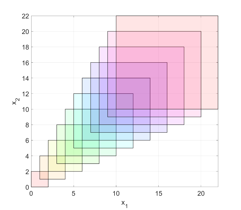
(a)

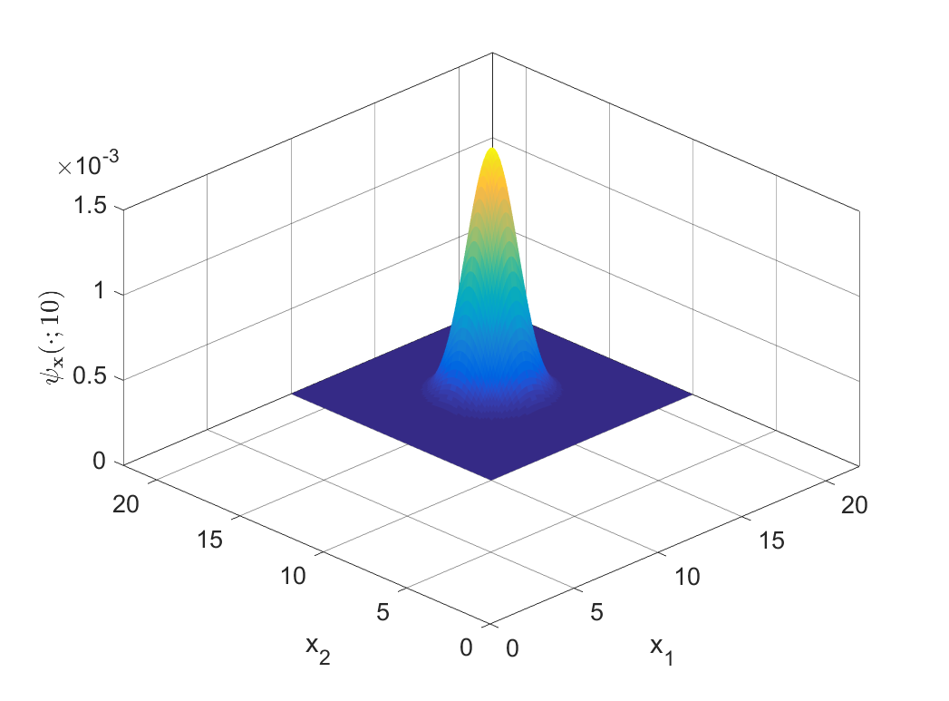
(b)

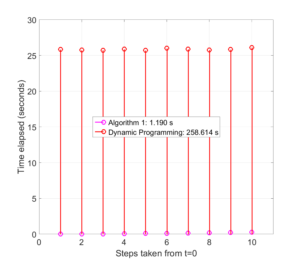
(c)

Figure 1: (a) Forward stochastic reach sets over time, (b) forward stochastic reach probability measure at $t=10$, (c) comparison of run times for Algorithm 1 and the dynamic programming approach. The analysis was done for the system given in (11).

The dynamic programming formulation provided in [30] computes the backward stochastic reachable set for control objectives involving safety. It allows for calculation of either stochastic reachable or stochastic viable sets, and simultaneously constructs an optimal control input. While Problem 1 can be posed as a backward reach problem when the dynamics are reversed in time (subject to the existence of the backward dynamics, when 1) $f(\cdot)$ is invertible, and 2) $\boldsymbol{v}[t]$ is an i.i.d process) [13], the solution to Problem 1 does not require computation of the optimal control action, significantly simplifying calculation. Algorithm 1 also iterates over only those states for which the FSRPM is positive. Therefore, at every time instant $t$, it propagates the dynamics over a smaller region of the state space $\mathrm{FSReach}(t,\mathcal{I})$ as compared to dynamic programming.

To demonstrate, consider a point mass dynamics discretized in time with velocities drawn from a truncated Gaussian distribution,

$$\boldsymbol{x}[t+1] =\boldsymbol{x}[t]+B_{\mathrm{ex,PM}}\boldsymbol{w}[t]$$ (11)

$$\boldsymbol{w}[t] \sim\mathcal{N}_{\mathrm{truncated,\mathcal{W}}}(\bar{\mu},\Sigma)$$

with state $\boldsymbol{x}[t]\in\mathbb{R}^{2}$, disturbance $\boldsymbol{w}[t]$ is a random vector taking values in $[1,2]^{2}$ following a truncated Gaussian density with mean $\bar{\mu}=[1.5\ 1.5]^{\top}$ and covariance matrix $\Sigma=0.1I_{2}$ and $B_{\mathrm{ex,PM}}=I_{2}$. We define the initial set as $\mathcal{I}=[0,2]^{2}$, and $\psi_{\boldsymbol{x}[0]}$ as a uniform distribution over $\mathcal{I}$. We use Algorithm 1 to compute $\mathrm{FSReach}(t,\mathcal{I})$ and $\psi_{\boldsymbol{x}}[\cdot;t]$ for $t\in[0,10]$ seconds. Figure 1(a) shows the evolution of $\mathrm{FSReach}(\cdot,\mathcal{I})$ over time (plotted using MPT [28]), Figure 1(b) shows the FSRPM for the system at $t=10$ and Figure 1(c) compares the runtime of the Algorithm 1 with the dynamic programming approach, with gridding of the state-space and disturbance with a grid size of $0.1$ in each dimension.

All computations in this paper were performed using MATLAB on an Intel Core i7 CPU with 2.10GHz clock rate and 8 GB RAM.

III-C Rigid body obstacles

We first extend the FSR set from point-mass obstacles (Subsection III-A) to rigid body obstacles.

Presume that the center of mass (referred to as the center, in shorthand) of the rigid body obstacle is described by $\boldsymbol{x}[\cdot]$. The set $O(\boldsymbol{x}[t])\subseteq\mathcal{X}$ describes set of states occupied by the obstacle at time $t$ when the obstacle’s center is $\boldsymbol{x}[t]$, that is, $O(\boldsymbol{x}[t])=\{y\>|\>h(y-\boldsymbol{x})\geq 0\}$ for some function $h:\mathbb{R}^{n}\rightarrow\mathbb{R}$ which implicitly describes the geometry of the obstacle. For example, for a unit square obstacle, one possible geometry function is $h(z)=1-\|z\|_{\infty}$.

We define an occupancy function of an obstacle $\phi^{r}_{\boldsymbol{x}}(\bar{y};t):\mathcal{X}\times[0,T]\rightarrow[0,1]$ to evaluate the probability of a point $\bar{y}\in\mathcal{X}$ being covered by the rigid body obstacle.

$$\phi_{\boldsymbol{x}}^{r}(\bar{y};t) =\psi_{\boldsymbol{x}}[\left\{\bar{z}\in\mathrm{FSReach}(t,\mathcal{I})|\bar{y}\in O(\bar{z})\right\};t]$$

$$=\sum_{\bar{z}\in\mathrm{FSReach}(t,\mathcal{I})}\psi_{\boldsymbol{x}}[\bar{z};t]\textbf{1}_{O(\bar{z})}(\bar{y}).$$ (12)

The description (12) follows from the inclusion-exclusion principle and the observation that the states of the rigid body centers are mutually exclusive events.

The occupancy function provides the collision probability with the rigid body obstacle. Note that the occupancy function is not a probability measure since $\sum_{\bar{y}\in\mathcal{X}}\phi_{\boldsymbol{x}}^{r}(\bar{y};t)\neq 1$. Also, the occupancy function lies in the interval $[0,1]$ since it is a sum of nonnegative numbers, and it is upper bounded by $\sum_{\bar{z}\in\mathrm{FSReach}(t,\mathcal{I})}\psi_{\boldsymbol{x}}[\bar{z};t]=1$.

We denote the $\alpha$-superlevel set of the occupancy function as

$$S_{\alpha}(t;\phi^{r}_{\boldsymbol{x}}) =\{\bar{y}\in\mathcal{X}|\phi^{r}_{\boldsymbol{x}}(\bar{y};t)\geq\alpha\}$$ (13)

For $\alpha>0$, $S_{\alpha}(t;\phi^{r}_{\boldsymbol{x}})$ is the “avoid” set for obstacle avoidance problems when probabilistic safety must be assured with at least likelihood $\alpha$. Note that $S_{0}(t;\phi^{r}_{\boldsymbol{x}})$ is equivalent to the conservative avoid set generated by worst-case reachability formulations [8, 9, 10, 11].

To utilize existing integer-programming based obstacle avoidance methods, we must have $\alpha$-superlevel sets of the occupancy function to be convex, or a union of convex sets.

We first define a function $D_{j}(\alpha,t)$ which describes the underlying cause of an occupancy function taking a value above the threshold $\alpha$. Given $\mathrm{FSReach}(t,\mathcal{I})$, let

$$D_{j}(\alpha,t) =\{\bar{z}_{k}\in\mathrm{FSReach}(t,\mathcal{I}):\sum_{k}\psi_{\boldsymbol{x}}[\bar{z}_{k};t]>\alpha$$

$$\text{and}\cap_{k}O(\bar{z}_{k})\neq\emptyset\}$$ (14)

$$j \in\{1,2,3...2^{|\mathrm{FSReach}(t,\mathcal{I})|}\}$$

be a set of possible rigid body centers, whose corresponding rigid bodies create overlap with an associated probability of obstacle occupancy greater than $\alpha$ (12). We denote $\mathscr{D}_{z}(\alpha,t)$ the collection of all such sets at time $t$.

To demonstrate, consider the scenario shown in Figure 2. Overlap in possible obstacle positions $\bar{z}_{1},\bar{z}_{2}$ generates a region of the state-space where likelihood of collision is higher than $\alpha$, even though $\psi_{\boldsymbol{x}}[\bar{z}_{1};t],\psi_{\boldsymbol{x}}[\bar{z}_{2};t]<\alpha$. We denote this region, as well as other regions (e.g., $\psi_{\boldsymbol{x}}[\bar{z}_{3};t]$) with likelihood higher than $\alpha$ through $D_{1}(\alpha,t)=\{\bar{z}_{1},\bar{z}_{2}\}$ and $D_{2}(\alpha,t)=\{\bar{z}_{3}\}$. Essentially, $D_{j}(\alpha,t)$ identifies the relevant obstacles through their centers.

Proposition 1.

For a single rigid body $O(\cdot)$ that is convex, the $\alpha$-superlevel sets of the occupancy function $\phi^{r}_{\boldsymbol{x}}[\bar{y};t]$ (12) is a union of convex sets.

Proof: Define regions of overlap described by (14) for a given likelihood $\alpha$ and FSRPM $\psi_{\boldsymbol{x}}[\bar{y};t]$. Then,

$$S_{\alpha}(t;\phi_{\boldsymbol{x}}^{r}) =\bigcup_{D_{j}(\alpha,t)\in\mathscr{D}_{z}(\alpha,t)}\bigcap_{\bar{z}\in D_{j}(\alpha,t)}O(\bar{z})\subseteq\mathcal{X}$$ (15)

for $\bar{z}\in\mathcal{X}$. The proof is complete with the observation that intersection preserves convexity.   

Hence Proposition 1 solves Problem 2.

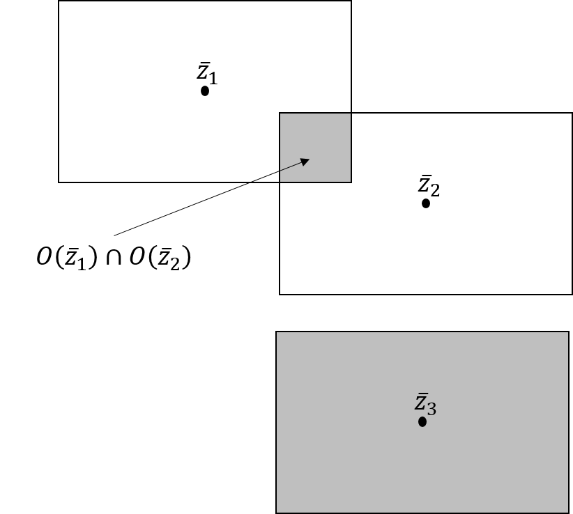
Figure 2: The shaded region has a likelihood of collision greater than $\alpha$. Consider a rigid-body obstacle, with possible obstacle locations $\bar{z}_{1},\bar{z}_{2},\bar{z}_{3}$ at time $t$. Presume that $\psi_{\boldsymbol{x}}[\bar{z}_{1};t]<\alpha$, $\psi_{\boldsymbol{x}}[\bar{z}_{2};t]<\alpha$, $\psi_{\boldsymbol{x}}[\bar{z}_{3};t]\geq\alpha$. Note that overlap between obstacles with centers $\bar{z}_{1}$ and $\bar{z}_{2}$ creates a likelihood greater than $\alpha$ for $O(\bar{z}_{1})\cap O(\bar{z}_{2})$, so that $\mathscr{D}_{z}(\alpha,t)=\{D_{1}(\alpha,t),D_{2}(\alpha,t)\}$ with $D_{1}(\alpha,t)=\{z_{1},z_{2}\}$ and $D_{2}(\alpha,t)=\{z_{3}\}$. Thus, $S_{\alpha}(t;\phi_{\boldsymbol{x}}^{r})=(O(\bar{z}_{1})\cap O(\bar{z}_{2}))\cup O(\bar{z}_{3})$.

Since the indicator function for the obstacle geometry in (12) can be equivalently expressed as $\textbf{1}_{O(\bar{z})}(\bar{y})=\textbf{1}_{O(0)}(\bar{y}-\bar{z})$, the occupancy function (12) can be re-written as

$$\phi_{\boldsymbol{x}}^{r}(\bar{y};t) =\sum_{\bar{z}\in\mathrm{FSReach}(t,\mathcal{I})}\psi_{\boldsymbol{x}}[\bar{z};t]\textbf{1}_{O(0)}(\bar{y}-\bar{z})$$

$$=\left(\psi_{\boldsymbol{x}}[\cdot;t]\ast\textbf{1}_{O(0)}(\cdot)\right)(\bar{y})$$ (16)

Equation (16) is similar to the concept of blurring in image processing, in which an image (in our case, $\psi_{\boldsymbol{x}}[\cdot;t]$), is convoluted with a shift-invariant point spread function, (in our case, $\textbf{1}_{O(0)}(\cdot)$). Such a formulation enables potential use of tools from image processing for the computation of $\phi_{\boldsymbol{x}}^{r}[\cdot;t]$ and its support for rigid body obstacles.

Now, we analyze the convexity property of (13) for multiple moving obstacles. For $N_{\mathrm{obs}}$ homogeneous obstacles, we denote the concatenated random vector of obstacle centers as $\boldsymbol{X}=[\boldsymbol{x}_{1}\ \boldsymbol{x}_{2}\ \ldots\ \boldsymbol{x}_{N_{\mathrm{obs}}}]\in\mathcal{X}^{N_{\mathrm{obs}}}$. We presume that the obstacles do not interact with each other, and hence are stochastically independent. For a given obstacle characterization $Z=[\bar{z}_{1}\ \bar{z}_{2}\ \ldots\ \bar{z}_{N_{\mathrm{obs}}}]\in\mathcal{X}^{N_{\mathrm{obs}}}$, the forward reach set and the probability measure of the obstacle configuration are described by

$$\mathrm{FSReach}_{\boldsymbol{X}}(t,\mathcal{I}) =\bigtimes_{i=1}^{N_{\mathrm{obs}}}\mathrm{FSReach}_{\boldsymbol{x}_{i}}(t,\mathcal{I})$$ (17)

$$\psi_{\boldsymbol{X}}[Z;t] =\prod_{i=1}^{N_{\mathrm{obs}}}\psi_{\boldsymbol{x}_{i}}[\bar{z}_{i};t].$$ (18)

Computation of (17), (18) relies on Algorithm 1 to compute (9), (10) for each obstacle individually.

We then define the joint occupancy function $\phi_{\boldsymbol{X}}^{r}(\bar{y},t):\mathcal{X}\times[0,T]\rightarrow[0,1]$ for a group of obstacles as the probability of any obstacle in the group occupying a state $\bar{y}$. Because of the mutual exclusivity of the configurations, the joint occupancy function is described by

$$\phi_{\boldsymbol{X}}^{r}(\bar{y};t) =\sum_{Z\in\mathrm{FSReach}_{\boldsymbol{X}}(t,\mathcal{I})}\psi_{\boldsymbol{X}}[Z;t]\textbf{1}_{\overline{O}(Z)}(\bar{y})$$ (19)

with $\overline{O}(Z)=\cup_{i=1}^{N_{\mathrm{obs}}}O(\bar{z}_{i})$. Similarly to (14), we define $\bar{D}_{j}(\alpha,t)$ as the sets of configurations, $j\in\{1,2,3,...,2^{|\mathrm{FSReach}_{\boldsymbol{X}}(t,\mathcal{I})|}\}$, whose probability of occurrence is greater than $\alpha$ and the resulting overlap is non-empty, and define $\mathscr{D}_{Z}(\alpha,t)$ as the collection of such sets for a given time $t$ in the configuration space $Z$.

Using an approach similar to that of Proposition 1, we can show that the $\alpha$ superlevel set of $\phi_{\boldsymbol{X}}^{r}(\bar{y};t)$ is

$$S_{\alpha}(t;\phi_{\boldsymbol{X}}^{r}) =\bigcup_{\bar{D}_{j}(\alpha,t)\in\mathscr{D}_{Z}(\alpha,t)}\bigcap_{Z\in\bar{D}_{j}(\alpha,t)}\bigcup_{i=1}^{N_{\mathrm{obs}}}O(\bar{z}_{i}).$$ (20)

Note that for $N_{\mathrm{obs}}=1$, (20) reduces to (15), as expected. We see from (20) that the avoid set for multiple moving obstacles is in general non-convex, and cannot be expressed as a union of convex avoid sets. Thus, to utilize integer programming based methods, the sets $S_{\alpha}(t;\phi_{\boldsymbol{X}}^{r})$ at every $t$ must be overapproximated as a union of convex sets. Although this is typically computationally expensive, we provide one such method in the next Section.

An alternative interpretation of (19) can be given by using events $\mathcal{E}_{i}$, which occur when $\mathbf{1}_{O(\boldsymbol{x}^{i})}(\bar{y})=1$. Essentially, the event $\mathcal{E}_{i}$ corresponds to the $i^{\mathrm{th}}$ obstacle occupying the state $\bar{y}\in\mathcal{X}$. Note that the event $\mathcal{E}_{i}$ depends only on the state of $i^{\mathrm{th}}$ obstacle center, and does not provide any restrictions on the centers of other obstacles in the configuration. Equation (19) can be rewritten as

$$\phi_{\boldsymbol{X}}^{r}(\bar{y};t) =\mathbb{E}_{\boldsymbol{X}}^{t}\left[\textbf{1}_{\overline{O}(Z)}(\bar{y})\right]=\mathbb{P}_{\boldsymbol{X}}^{t}\left\{\bigcup_{i=1}^{N_{\mathrm{obs}}}\mathcal{E}_{i}\right\}$$ (21)

where $\mathbb{P}_{\boldsymbol{X}}^{t}$ denotes the joint probability measure associated with the configuration of the obstacles. Such a formulation is important for constructing an overapproximation of avoid set (and hence under-approximation of the collision-free set) that can be represented as the union of convex sets.

We define “safety” as ensuring that the probability of collision of the robot with any of the obstacles at any given time $t\in[0,T]$ is less than a specified threshold, $\alpha\in[0,1]$. We define the safe set $\mathrm{SafeSet}[t;\alpha]$ as the complement of the set $S_{\alpha}(t;\phi_{\boldsymbol{X}}^{r})$, such that

$$\mathrm{SafeSet}[t;\alpha] =\left\{\bar{y}\in\mathcal{X}\middle|\phi^{r}_{\boldsymbol{X}}(\bar{y})<\alpha\right\}=\mathcal{X}\setminus S_{\alpha}(t;\phi_{\boldsymbol{X}}^{r}).$$ (22)

Note that (22) is not guaranteed to be convex even if the obstacles are convex. Convexification methods [31] for evaluation of (20) and (22) would need to be implemented online, and are computationally expensive. Hence, for computational tractability, at each time step $t$, we underapproximate (22) using the definition of $\phi_{\boldsymbol{X}}^{r}$ in (21),

$$\underline{\mathrm{SafeSet}}[t;\alpha] =\bigcap_{i=1}^{N_{\mathrm{obs}}}\left\{\bar{y}\in\mathcal{X}\middle|\mathbb{P}_{\boldsymbol{X}}^{t}(\mathcal{E}_{i})<\frac{\alpha}{N_{\mathrm{obs}}}\right\}.$$ (23)

Since $\mathbb{P}(\cup_{i}\mathcal{E}_{i})\leq\sum_{i}\mathbb{P}(\mathcal{E}_{i})$,

$$\underline{\mathrm{SafeSet}}[t;\alpha]\subseteq\mathrm{SafeSet}[t;\alpha].$$ (24)

By construction, $\mathcal{E}_{i}$ restricts the state of the $i^{\mathrm{th}}$ obstacle alone. Therefore, (23) can be computed using (15) as

$$\underline{\mathrm{SafeSet}}[t;\alpha] =\bigcap_{i=1}^{N_{\mathrm{obs}}}\left(\mathcal{X}\setminus S^{i}_{\frac{\alpha}{N_{\mathrm{obs}}}}(t;\phi_{\boldsymbol{x}}^{r})\right).$$ (25)

$$=\mathcal{X}\setminus\bigcup_{i=1}^{N_{\mathrm{obs}}}\left(S^{i}_{\frac{\alpha}{N_{\mathrm{obs}}}}(t;\phi_{\boldsymbol{x}}^{r})\right)$$ (26)

Hence Problem 3 is solved, since $\cup_{i=1}^{N_{obs}}S^{i}_{\frac{\alpha}{N_{\mathrm{obs}}}}(t;\phi_{\boldsymbol{x}}^{r})$ in (26) is an overapproximation that can be written as a union of convex sets. Here, $S^{i}_{\frac{\alpha}{N_{\mathrm{obs}}}}$ is the $\left(\frac{\alpha}{N_{\mathrm{obs}}}\right)$-superlevel set of the occupancy function of the $i^{th}$ obstacle at time $t$. Note that $S^{i}_{\frac{\alpha}{N_{\mathrm{obs}}}}(\cdot,t)$ for every $t=[0,1,\cdots,T]$ and for every obstacle $i$ can be computed offline, and hence any form of online convexification is avoided with this overapproximation.

The particular under-approximation will be specific to the problem at hand. In general, integer variables must be introduced to accommodate each obstacle, and the sets in (20) approximated via a set of linear constraints. We demonstrate this approach in the next Section.

IV Application to obstacle avoidance

We now consider the specific problem of robot navigation in an environment with ${N_{\mathrm{obs}}}$ rigid body obstacles moving in straight lines with stochastic velocities. We use integer programming [2, 4] in a receding horizon control framework to drive the robot to the desired goal $\bar{x}_{G}\in\mathcal{X}$ in finite time, while ensuring a probabilistic guarantee of safety. We presume that robot and obstacle positions are known at each instant.

We model the robot as a point mass under state-feedback control

$$\bar{x}_{R}[t+1] =\bar{x}_{R}[t]+B_{R}u[t]$$ (27)

with state $\bar{x}_{R}[t]\in\mathcal{X}=\mathbb{R}^{2\times 1}$ that represents robot position and input $u[t]\in\mathcal{U}\subseteq\mathbb{R}^{2}$. The input matrix is $B_{R}=T_{s}I_{2}$, with sampling time $T_{s}$.

The obstacles have identical dynamics and do not interact with each other, and have rigid bodies that are unit boxes with fixed heading. In the absence of any rotation, the obstacle position is completely characterized by the dynamics of the center. The dynamics of the center of the $k^{\mathrm{th}}$ obstacle is described

$$\boldsymbol{x}^{k}_{o}[t+1] =\boldsymbol{x}^{k}_{o}[t]+B_{o}\boldsymbol{w}^{k}[t]$$ (28)

with state $\boldsymbol{x}^{k}_{o}[t]\in\mathcal{X}$, stochastic velocity $\boldsymbol{w}^{k}[t]\in\mathcal{W}_{o,d}^{2}$ described by an i.i.d. process, and disturbance matrix $B_{o}=B_{R}$. The disturbance set $\mathcal{W}_{o,d}\subseteq\mathbb{R}$ describes possible obstacle velocities. We define the probability mass function of the velocity vector $\boldsymbol{w}^{k}$ to be $\psi_{\boldsymbol{w}^{k}}[z]$, hence the state $\boldsymbol{x}_{o}^{k}[t]$ is a random vector in the probability space $(\mathcal{X},\sigma(\mathcal{X}),\mathbb{P}_{\boldsymbol{x}_{o}}^{t,\bar{x}_{o},k})$ for a given initial position $\bar{x}_{o}\in\mathcal{X}$. The probability measure associated with $k^{\mathrm{th}}$ obstacle $\mathbb{P}_{\boldsymbol{x}_{o}}^{t,\bar{x}_{o},k}$ is induced from the product measure associated with $\psi_{\boldsymbol{w}^{k}}$ and depends on the initial position $\bar{x}_{0}$ and time $t$.

Prob A: $$\begin{array}[]{rcl}\underset{\pi}{\operatorname{minimize}}&&J(\pi;\bar{x}_{R}[0],\boldsymbol{X}[\cdot])=\sum_{t=0}^{T}\left\{(\bar{x}_{R}[t]-\bar{x}_{G})^{\top}Q(\bar{x}_{R}[t]-\bar{x}_{G})+\pi(t,\bar{x}_{R}[t],\boldsymbol{X}[t])^{T}R^{u}(t,\bar{x}_{R}[t],\boldsymbol{X}[t])\right\}\\ \mbox{subject to}&&\left\{\begin{array}[]{rll}\bar{x}_{R}[t]&=\bar{x}_{R}[t-1]+B_{R}\pi(t,\bar{x}_{R}[t-1],\boldsymbol{X}[t])&t=1,\ldots,T,\\ \bar{x}_{R}[t]&\in\mathrm{SafeSet}[t;\alpha]&t=1,\ldots,T\\ \pi(\cdot)&\in\mathcal{M}\\ \end{array}\right.\end{array}$$ (34)

 

We wish to solve Problem Prob A. The control policy $\pi(t,\bar{x}_{R}[t],\boldsymbol{X}[t]):[0,T-1]\times\mathcal{X}^{1+N_{\mathrm{obs}}}\rightarrow\mathcal{U}$ is a state-feedback control with the set of feasible policies $\pi(\cdot)$ denoted by $\mathcal{M}$. Here, $Q$ and $R^{u}$ are symmetric positive definite matrices of appropriate dimensions.

A conservative solution to Problem Prob A can be found by solving the following optimization problem:

$$\begin{array}[]{rl}\mbox{Prob B:}&\begin{array}[]{rl}\mbox{minimize}&J(\pi;\bar{x}_{R}[0],\boldsymbol{X}[\cdot])\\ \mbox{subject to}&\left\{\begin{array}[]{rll}\bar{x}_{R}[t]&\mbox{ by \eqref{eq:robot_dyn_SIM1} with }\pi&\forall t\\ \bar{x}_{R}[t]&\in\underline{\mathrm{SafeSet}}[t;\alpha]&\forall t\\ \pi&\in\mathcal{M}&\\ \end{array}\right.\end{array}\end{array}$$ (41)

We replace the constraint $x_{R}[t]\in\underline{\mathrm{SafeSet}}[t;\alpha]$ in Problem Prob B by defining

$$K_{i}=\{\bar{y}\in\mathcal{X}|P_{i}\bar{y}\leq\bar{q}_{i},P_{i}\in\mathbb{R}^{n_{i}\times 2},\bar{q}_{i}\in\mathbb{R}^{n_{i}}\}$$ (42)

such that $\mathcal{X}\setminus(\cup_{i=1}^{N_{s}}K_{i})\subseteq\underline{\mathrm{SafeSet}}[t;\alpha]$, resulting in the following constraint set for $i=1,\ldots,N_{s}$:

$$\delta_{i,l} \in\{0,1\}, l=1,\ldots,n_{i}$$ (43a)

$$-\bar{p}_{i,l}[t]^{\top}\bar{x}_{R}[t] <-q_{i,l}[t]+M_{\mathrm{big}}\delta_{i,l}$$ (43b)

$$\sum_{l=1}^{n_{i}}\delta_{i,l} \leq(n_{i}-1)$$ (43c)

Here, $\bar{p}_{i,l}[t]$ and $q_{i,l}[t]$ are the $l^{th}$ row of matrix $P_{i}[t]$ and $l^{th}$ element of vector $\bar{q}_{i}[t]$ respectively. The term $M_{\mathrm{big}}$ is a large number that facilitates the constraint satisfaction. The constraint (43c) ensures that at least one of the binary variables $\delta_{i,l}=0$ for every $i$. This formulation ensures the robot avoids every avoid set $i=1,2,\cdots,N_{s}$.

We implement the problem with the following parameters: $T_{s}=0.2$, $T=50$, the stochastic speed set $\mathcal{W}_{o,d}=\{3,2.5,1.5,2,1,0.8,0.5,0.1\}$ m/s with probabilities $\psi_{\boldsymbol{w}^{k}}[z]\in\{0.05,0.05,0.30,0.20,0.25,0.10,0.04,0.01\}$.

The input space for the robot is $\mathcal{U}=[-0.2,1]\times[0.1,1]$, so that it cannot stop in the $y$-direction. Note that the average velocity of each obstacle is $1.476$ m/s while the maximum robot velocity in both directions is $1$ m/s, which is about two-thirds the obstacle’s maximum velocity. The robot is disadvantaged because it is slower than the obstacles.

To compute the forward stochastic reach sets and occupancy function, we discretize the state space with a resolution of $0.05$ and follow Algorithm 1. We use YALMIP [32] with the Gurobi [33] solver to solve Problem Prob B with the constraint in (43). The computation took approximately $0.04$ seconds to complete.

Results are shown in Figure 3 from a single initial obstacle-robot configuration. We compare our probabilistic approach with the case in which $\alpha=0$, which is equivalent to the result from the conservative min-max solution in [14, 8, 9, 10, 11]. Note that the min-max solution becomes infeasible at approximately $1.8$ seconds (10 time steps). With $\alpha=0.045$, meaning that obstacles should be avoided with likelihood of 0.95, feasible solutions are found for the entire time horizon.

Figure 3: Snapshots of stochastically moving obstacles and robots and their trajectories. The red robot’s trajectory is indicated by the blue line, and the pink robot’s trajectory is indicated by the cyan line. The red robot uses $\alpha=0.045$ while the pink robot uses $\alpha=0$ (the min-max problem).

V Conclusions and Future work

This paper provides a method for computing the forward stochastic reachable set and probability measure, with application to obstacle avoidance. The method handles uncontrolled nonlinear systems, or systems with a known controller, as well as an affine disturbance that captures the stochastic element. We have described how the forward stochastic reachable set and probability measure can be used to generate an occupancy constraint that can be written as a union as convex sets, and hence is amenable to use in existing integer programming based methods for collision avoidance over a finite horizon.

Future work includes the extension to problems with an uncountable sample space, and development of computationally efficient online control methods. We also anticipate application of these techniques to (dynamic) target reaching problems.

References

- [1] E. Rimon and D. E. Koditschek, “Exact robot navigation using artificial potential functions,” IEEE Transactions on robotics and automation, vol. 8, no. 5, pp. 501–518, 1992.
- [2] T. Schouwenaars, É. Féron, and J. How, “Safe receding horizon path planning for autonomous vehicles,” in Conference on Communication, Control, and Computing, vol. 40, pp. 295–304, The University; 1998, 2002.
- [3] T. Schouwenaars, B. De Moor, E. Feron, and J. How, “Mixed integer programming for multi-vehicle path planning,” in European Control Conference, pp. 2603–2608, 2001.
- [4] D. Mellinger, A. Kushleyev, and V. Kumar, “Mixed-integer quadratic program trajectory generation for heterogeneous quadrotor teams,” in IEEE International Conference on Robotics and Automation, pp. 477–483, 2012.
- [5] S. Karaman and E. Frazzoli, “Sampling-based algorithms for optimal motion planning,” The International Journal of Robotics Research, vol. 30, no. 7, pp. 846–894, 2011.
- [6] H.-T. Chiang, N. Rackley, and L. Tapia, “Stochastic ensemble simulation motion planning in stochastic dynamic environments,” in IEEE/RSJ International Conference on Intelligent Robots and Systems (IROS), pp. 3836–3843, 2015.
- [7] P. Fiorini and Z. Shiller, “Motion planning in dynamic environments using velocity obstacles,” The International Journal of Robotics Research, vol. 17, no. 7, pp. 760–772, 1998.
- [8] A. Wu and J. P. How, “Guaranteed infinite horizon avoidance of unpredictable, dynamically constrained obstacles,” Autonomous Robots, vol. 32, no. 3, pp. 227–242, 2012.
- [9] C. F. Chung, T. Furukawa, and A. H. Goktogan, “Coordinated control for capturing a highly maneuverable evader using forward reachable sets,” in IEEE International Conference on Robotics and Automation, pp. 1336–1341, 2006.
- [10] M. Althoff and J. M. Dolan, “Online verification of automated road vehicles using reachability analysis,” IEEE Transactions on Robotics, vol. 30, no. 4, pp. 903–918, 2014.
- [11] Y. Lin and S. Saripalli, “Collision avoidance for uavs using reachable sets,” in International Conference on Unmanned Aircraft Systems, pp. 226–235, 2015.
- [12] N. E. Du Toit and J. W. Burdick, “Robot motion planning in dynamic, uncertain environments,” IEEE Transactions on Robotics, vol. 28, no. 1, pp. 101–115, 2012.
- [13] I. M. Mitchell, “Comparing forward and backward reachability as tools for safety analysis,” in Hybrid systems: computation and control, pp. 428–443, Pisa, Italy: Springer, 2007.
- [14] I. M. Mitchell, A. M. Bayen, and C. J. Tomlin, “A time-dependent hamilton-jacobi formulation of reachable sets for continuous dynamic games,” IEEE Transactions on automatic control, vol. 50, no. 7, pp. 947–957, 2005.
- [15] J. F. Fisac, M. Chen, C. J. Tomlin, and S. S. Sastry, “Reach-avoid problems with time-varying dynamics, targets and constraints,” in Hybrid Systems: Computation and Control, pp. 11–20, 2015.
- [16] J. Ding and C. J. Tomlin, “Robust reach-avoid controller synthesis for switched nonlinear systems,” in IEEE Conference on Decision and Control, pp. 6481–6486, 2010.
- [17] R. Takei, H. Huang, J. Ding, and C. J. Tomlin, “Time-optimal multi-stage motion planning with guaranteed collision avoidance via an open-loop game formulation,” in IEEE International Conference on Robotics and Automation, pp. 323–329, 2012.
- [18] K. Margellos and J. Lygeros, “Hamilton-Jacobi formulation for reach-avoid problems with an application to air traffic management,” American Control Conference, pp. 3045–3050, 2010.
- [19] J. Ding, E. Li, H. Huang, and C. Tomlin, “Reachability-based synthesis of feedback policies for motion planning under bounded disturbances,” in IEEE International Conference on Robotics and Automation, pp. 2160–2165, 2011.
- [20] J. H. Gillula, G. M. Hoffmann, H. Haomiao, M. P. Vitus, and C. J. Tomlin, “Applications of hybrid reachability analysis to robotic aerial vehicles,” The International Journal of Robotics Research, pp. 335–354, 2011.
- [21] M. Chen, Q. Hu, C. Mackin, J. F. Fisac, and C. J. Tomlin, “Safe platooning of unmanned aerial vehicles via reachability,” in IEEE Conference on Decision and Control, pp. 4695–4701, 2015.
- [22] N. Malone, K. Lesser, M. Oishi, and L. Tapia, “Stochastic reachability based motion planning for multiple moving obstacle avoidance,” in Hybrid systems: computation and control, pp. 51–60, 2014.
- [23] H.-T. Chiang, N. Malone, K. Lesser, M. Oishi, and L. Tapia, “Aggressive moving obstacle avoidance using a stochastic reachable set based potential field,” in Algorithmic Foundations of Robotics XI, pp. 73–89, Springer, 2015.
- [24] G. S. Aoude, B. D. Luders, J. M. Joseph, N. Roy, and J. P. How, “Probabilistically safe motion planning to avoid dynamic obstacles with uncertain motion patterns,” Autonomous Robots, vol. 35, no. 1, pp. 51–76, 2013.
- [25] G. Best and R. Fitch, “Bayesian intention inference for trajectory prediction with an unknown goal destination,” in IEEE/RSJ International Conference on Intelligent Robots and Systems, pp. 5817–5823, 2015.
- [26] F. Havlak and M. Campbell, “Discrete and continuous, probabilistic anticipation for autonomous robots in urban environments,” IEEE Transactions on Robotics, vol. 30, no. 2, pp. 461–474, 2014.
- [27] M. Kvasnica, B. Takács, J. Holaza, and D. Ingole, “Reachability analysis and control synthesis for uncertain linear systems in mpt,” IFAC Symposium on Robust Control Design, vol. 48, no. 14, pp. 302–307, 2015.
- [28] M. Herceg, M. Kvasnica, C. Jones, and M. Morari, “Multi-Parametric Toolbox 3.0,” in European Control Conference, (Zürich, Switzerland), pp. 502–510, July 17–19 2013.
- [29] A. A. Kurzhanskiy and P. Varaiya, “Ellipsoidal toolbox,” Tech. Rep. UCB/EECS-2006-46, EECS Department, University of California, Berkeley, 2006.
- [30] S. Summers and J. Lygeros, “Verification of discrete time stochastic hybrid systems: A stochastic reach-avoid decision problem,” Automatica, vol. 46, no. 12, pp. 1951–1961, 2010.
- [31] B. Açıkmeşe, J. M. Carson, and L. Blackmore, “Lossless convexification of nonconvex control bound and pointing constraints of the soft landing optimal control problem,” IEEE Transactions on Control Systems Technology, vol. 21, no. 6, pp. 2104–2113, 2013.
- [32] J. Lofberg, “Yalmip: A toolbox for modeling and optimization in matlab,” in IEEE International Symposium on Computer Aided Control Systems Design, pp. 284–289, 2004.
- [33] G. Optimization, “Gurobi optimizer reference manual,” 2015.