Magnetic concentrations in stratified turbulence: the negative effective magnetic pressure instability

Abstract

In the presence of strong density stratification, hydromagnetic turbulence attains qualitatively new properties: the formation of magnetic flux concentrations. We review here the theoretical foundations of this mechanism in terms of what is now called the negative effective magnetic pressure instability. We also present direct numerical simulations of forced turbulence in strongly stratified layers and discuss the qualitative and quantitative similarities with corresponding mean-field simulations. Finally, the relevance to sunspot formation is discussed.

1 Introduction

Magnetohydrodynamic (MHD) turbulence has been studied for a long time, starting with early work on the energy spectrum [1, 2] in the 1960s. In many subsequent studies, the effect of gravity was either not considered or it was thought to being just part of the convective driving of the turbulence. The idea that gravity itself could be responsible for causing qualitatively new phenomena in turbulence hardly occurred. This has changed dramatically in just the last few years. An important example is the combined action of gravity with an imposed vertical magnetic field. This drives cross helicity [3], which is an important invariant in ideal MHD. Another example, that will form the main focus of this review, is the spontaneous production of large-scale magnetic flux concentrations in small-scale MHD turbulence by the negative effective magnetic pressure instability (NEMPI), which has its roots in early analytic work [4, 5, 6, 7, 8, 9], and emerged recently as a pronounced effect in direct numerical simulations (DNS); see Refs. [10, 11, 12, 13, 14].

In MHD turbulence there is another important effect that leads to the formation of magnetic structures, namely the dynamo instability. In that case, gravity is unimportant for structure formation, although it does often play a role in driving turbulence, for example through convection. Thus, the dynamo effect must not be confused with the type of structure formation where gravity is a crucial ingredient. Furthermore, convection leads to converging downdrafts that enhance the magnetic field by compression and tend to expel it from diverging flow regions [15, 16].

NEMPI, or some similar process, in conjunction with dynamo theory, is one of the contenders in explaining the surface activity of the Sun and other stars. The other main contender is the rising flux tube scenario by which strong coherent flux tubes are being built in the tachocline [17, 18, 19], which is the shear layer between the convection zone and the radiative interior. However, the helioseismic signatures of such a scenario [20] have not been detected [21]. Observations are more consistent with a gradual build-up of an active region on the timescale of one to two days [22]. An entirely different kinematic process that can form magnetic concentrations is flux expulsion, by which magnetic fields are expelled from regions of rapid motion. A classical example is a convection cell where magnetic field is swept away from the diverging upflows of granules into intergranular lanes and vertices [23, 24]. Results from relatively weakly stratified numerical simulations of convection can be explained by this process [16, 25, 26], but its role in the presence of strong stratification has not yet been studied. Numerical simulations with realistic surface physics have successfully produced active region formation from an unstructured initial magnetic field [27], but it is still a large leap to modeling actual sunspots [28].

Meanwhile, several simulations have displayed spontaneous magnetic structure formation. Some of them involve turbulent convection [27, 16, 29, 30, 31], or a stably stratified polytropic atmosphere [32], so it remains to be clarified, whether gravity plays a direct role, or whether the magnetic field concentrations are mainly the result of converging downdrafts. Other simulations involve forced turbulence in isothermally stratified domains, where no thermally driven convection is possible [10, 11, 12, 13, 14, 33, 34, 35], and yet one finds the formation of large-scale magnetic structures. What is remarkable is that these structures extend over the scale of many turbulent eddies. This property suggests that they should be amenable to a mean-field treatment involving averaged, effective equations.

A mean-field approach relevant for describing magnetic effects on the mean flow was developed nearly three decades ago [4, 5, 6, 7, 8, 9], but only in recent years, with the assistance of DNS, has it gained sufficient attention. In the following, we review the essential properties of NEMPI, discuss analytical approaches to the understanding of the behavior in the presence of either horizontal or vertical magnetic fields, and then turn to DNS whose results can be understood in terms of NEMPI.

2 The physics of NEMPI

2.1 Effective magnetic pressure

In the following, we discuss the formation of magnetic structures through a reduction of turbulent pressure by the large-scale magnetic field. For large magnetic Reynolds numbers this suppression of the turbulent pressure can be large enough so that the effective large-scale magnetic pressure (the sum of non-turbulent and turbulent contributions to the large-scale magnetic pressure) becomes negative. The essence of this effect is as follows. The momentum equation describing the plasma motions reads

$${\partial\over\partial t}\rho U_{i}=-{\partial\over\partial x_{j}}\Pi_{ij}+\rho\,g_{i},$$ (1)

where ${\bm{g}}$ is the acceleration due to gravity,

$$\Pi_{ij}=\rho\,U_{i}U_{j}+\delta_{ij}\left(p+\frac{1}{2}{\bm{B}}^{2}\right)-B_{i}B_{j}-2\nu\rho\,{\sf S}_{ij},$$ (2)

is the momentum stress tensor, $\bm{U}$ and ${\bm{B}}$ are the velocity and magnetic fields, $p$ and $\rho$ are the fluid pressure and density, $\delta_{ij}$ is the Kronecker tensor, $\nu$ is the kinematic viscosity, and ${\sf S}_{ij}={\textstyle{1\over 2}}(\partial_{i}U_{j}+\partial_{j}U_{i})-{\textstyle{1\over 3}}\delta_{ij}{\bm{\nabla}}\cdot\bm{U}$ is the trace-free rate of strain tensor. We have adopted units where the vacuum permeability $\mu_{0}$ is set to unity.

Neglecting correlations between velocity and density fluctuations for low-Mach number turbulence, the averaged momentum equation is

$${\partial\over\partial t}\overline{\rho}\,\overline{U}_{i}=-{\partial\over\partial x_{j}}\overline{\Pi}_{ij}+\overline{\rho}\,g_{i},$$ (3)

where $\overline{\rho}$ is the mean fluid density, $\overline{\bm{U}}$ is the mean fluid velocity, $\overline{\Pi}_{ij}=\overline{\Pi}_{ij}^{\rm m}+\overline{\Pi}_{ij}^{\rm f}$ is the mean momentum stress tensor split into contributions resulting entirely from the mean field (indicated by superscript m) and those of the fluctuating field (indicated by superscript f). In the following, the fluctuations of velocity and magnetic field are defined as $\bm{u}=\bm{U}-\overline{\bm{U}}$ and $\bm{b}={\bm{B}}-{\overline{\bm{B}}}$, respectively, where ${\overline{\bm{B}}}$ is the mean magnetic field. The tensor $\overline{\Pi}_{ij}^{\rm m}$ has the same form as equation (2), but all quantities have now attained an overbar, i.e.

$$\overline{\Pi}_{ij}^{\rm m}=\overline{\rho}\,\overline{U}_{i}\overline{U}_{j}+\delta_{ij}\left(\overline{p}+\frac{1}{2}\overline{{\bm{B}}}^{2}\right)-\overline{B}_{i}\overline{B}_{j}-2\nu\overline{\rho}\,\overline{\sf S}_{ij},$$ (4)

where $\overline{p}$ is the mean fluid pressure. The contributions $\overline{\Pi}_{ij}^{\rm f}$, which describe the effect of turbulence on the large-scale Lorentz force, are determined by

$$\overline{\Pi}_{ij}^{\rm f}=\overline{\rho}\,\overline{u_{i}u_{j}}+{\textstyle{1\over 2}}\overline{\bm{b}^{2}}\delta_{ij}-\overline{b_{i}b_{j}}.$$ (5)

The turbulent stress tensor, $\overline{\Pi}_{ij}^{\rm f}$, together with the stress tensor describing the mean field contributions, $\overline{\Pi}_{ij}^{\rm m}$, comprise the total mean momentum tensor.

Let us first consider isotropic turbulence. The total (hydrodynamic plus magnetic) turbulent pressure $p_{\rm turb}$ (i.e., the isotropic part of $\overline{\Pi}_{ij}^{\rm f}$) is, in this case, given by [36, 37]

$$p_{\rm turb}=\frac{2}{3}E_{\rm K}+\frac{1}{3}E_{\rm M},$$ (6)

where $E_{\rm K}=\frac{1}{2}\rho\,\overline{{\bm{u}}^{2}}$ is the kinetic energy density of the turbulent (small-scale) motions, $E_{\rm M}=\overline{{\bm{b}}^{2}}/2$ is the energy density of the magnetic fluctuations. The different coefficients in the “turbulent” equation of state, equation (6), for the total turbulent pressure are caused by the fact that the contribution of velocity fluctuations to $p_{\rm turb}$ is determined by the Reynolds stresses, $\overline{u_{i}u_{j}}$, which, for isotropic turbulence, are $\overline{u_{i}u_{j}}=\frac{1}{3}\overline{{\bm{u}}^{2}}\,\delta_{ij}\equiv\frac{2}{3}(E_{\rm K}/\rho)\,\delta_{ij}$. On the other hand, the contribution of magnetic fluctuations to $p_{\rm turb}$ is determined by the Maxwell stresses, $M_{ij}\equiv\frac{1}{2}\overline{{\bm{b}}^{2}}\,\delta_{ij}-\overline{b_{i}b_{j}}$, where $\overline{b_{i}b_{j}}=\frac{1}{3}\overline{{\bm{b}}^{2}}\,\delta_{ij}$ for isotropic turbulence. In that case we have $M_{ij}=(\overline{{\bm{b}}^{2}}/6)\,\delta_{ij}\equiv\frac{1}{3}E_{\rm M}\,\delta_{ij}$.

In homogeneous turbulence with a uniform large-scale magnetic field, the total turbulent energy density $E_{T}=E_{\rm K}+E_{\rm M}$ is constant, because dissipation is compensated by a continuous supply of energy [8, 9], so

$$E_{\rm K}+E_{\rm M}={\rm const}{}.$$ (7)

This implies that a uniform large-scale magnetic field performs no work on the turbulence. It can only redistribute energy between hydrodynamic and magnetic fluctuations. Equation (7) is a steady-state solution for the budget equation for the total turbulent energy density for a time-independent energy source of homogeneous turbulence, $I_{T}$, with a zero mean velocity and weakly non-uniform mean magnetic field

$$\frac{\partial E_{T}}{\partial t}=I_{T}+\eta_{\rm t}\,\bm{\overline{}}{\bm{J}}^{2}-\frac{E_{T}}{\tau_{0}},$$ (8)

where ${\bm{\overline{J}}}={\bm{\nabla}}\times\overline{\bm{B}}$ is the mean current density, $\tau_{0}$ is the correlation time of the turbulent velocity field at the integral scale $\ell_{0}$ of turbulent motions, and $\eta_{\rm t}$ is the turbulent magnetic diffusion. The last term, $-E_{T}/\tau_{0}$, in the right-hand side of equation (8) determines the dissipation of the total turbulent energy for the large fluid and magnetic Reynolds numbers. Equations (6) and (7) allow us to determine the change of the total turbulent pressure $\delta p_{\rm turb}$ in terms of the change of magnetic energy density $\delta E_{\rm M}$,

$$\delta p_{\rm turb}=-\frac{1}{3}\,\delta E_{\rm M}.$$ (9)

Equation (9) implies that the total turbulent pressure is reduced when magnetic fluctuations are generated ($\delta E_{\rm M}>0$).

Let us now consider anisotropic turbulence with a preferred direction parallel to some unit vector $\hat{\bm{e}}$. Specifically, we assume the velocity to be given in the form ${\bm{u}}={\bm{u}}_{\perp}+u_{z}\hat{\bm{e}}$, where ${\bm{u}}_{z}=u_{z}\hat{\bm{e}}$ and ${\bm{u}}_{\perp}={\bm{u}}-{\bm{u}}_{z}$ are the velocities parallel and perpendicular to $\hat{\bm{e}}$. We characterize the degree of anisotropy by the parameter $\sigma=\overline{{\bm{u}}_{\perp}^{2}}/2\overline{{\bm{u}}_{z}^{2}}-1$. Thus, for isotropic three-dimensional turbulence we have $\sigma=0$, while for strongly anisotropic turbulence $\sigma$ is large. For two-dimensional turbulence (an extremely anisotropic case) the parameter $\sigma\to\infty$. We can then write

$$\overline{u_{i}u_{j}}=\frac{1}{3+2\sigma}\overline{{\bm{u}}^{2}}\,\left[\delta_{ij}+\sigma\left(\delta_{ij}-e_{i}e_{j}\right)\right],$$ (10)

$$\overline{b_{i}b_{j}}=\frac{1}{3+2\sigma}\overline{{\bm{b}}^{2}}\,\left[\delta_{ij}+\sigma\left(\delta_{ij}-e_{i}e_{j}\right)\right].$$ (11)

Substituting equations (10) and (11) into equation (5), the isotropic part of the tensor $\overline{\Pi}_{ij}^{\rm f}$, which yields the total turbulent pressure for anisotropic turbulence, becomes

$$p_{\rm turb}=\frac{2(1+2\sigma)}{3+2\sigma}E_{\rm K}+\frac{1}{3+2\sigma}E_{\rm M}.$$ (12)

The change of the total turbulent pressure $\delta p_{\rm turb}$ can then be written in terms of the change of magnetic energy density $\delta E_{\rm M}$ as

$$\delta p_{\rm turb}=-\frac{1+4\sigma}{3+2\sigma}\,\delta E_{\rm M}.$$ (13)

For strongly anisotropic turbulence with $\sigma\gg 1$ we have

$$\delta p_{\rm turb}=-2\,\delta E_{\rm M}.$$ (14)

Therefore, for strongly anisotropic turbulence the reduction of the total turbulent pressure by the large-scale magnetic field is six times larger in comparison with that for isotropic turbulence [see equations (9) and (14)].

The turbulent stress tensor, $\overline{\Pi}_{ij}^{\rm f}$, is split into parts that are independent of the mean magnetic field (they determine turbulent viscosity and background turbulent pressure), and parts that do depend on the mean magnetic field. In the presence of a non-zero mean magnetic field only the difference in the stress tensor,

$$\Delta\overline{\Pi}_{ij}^{{\rm f}}\equiv\overline{\Pi}_{ij}^{{\rm f},\overline{B}}-\overline{\Pi}_{ij}^{\rm f,0},$$ (15)

depends on the mean magnetic field ${\overline{\bm{B}}}$, where $\overline{\Pi}_{ij}^{\rm f,0}=\overline{\Pi}_{ij}^{\rm f}({\overline{\bm{B}}}=0)$. To parameterize the tensor $\Delta\overline{\Pi}_{ij}^{{\rm f}}$ we use symmetry arguments, which allow us to construct a symmetric tensor with two preferential directions along the mean magnetic field $\hat{\bm{\beta}}={\overline{\bm{B}}}/|{\overline{\bm{B}}}|$ and the gravity field $\hat{\bm{g}}={\bm{g}}/g$. Such a symmetric tensor should be a linear combination of symmetric tensors $\delta_{ij}$, $\hat{\beta}_{i}\hat{\beta}_{j}$ and $\hat{g}_{i}\hat{g}_{j}$. These arguments yield [9]

$$\Delta\overline{\Pi}_{ij}^{{\rm f}}=q_{\rm s}{\overline{\bm{B}}}^{2}\hat{\beta}_{i}\hat{\beta}_{j}-\,\Big{(}{\textstyle{1\over 2}}q_{\rm p}\,\delta_{ij}+q_{\rm g}\,\hat{g}_{i}\hat{g}_{j}\Big{)}{\overline{\bm{B}}}^{2},$$ (16)

where $q_{\rm s}$, $q_{\rm p}$, and $q_{\rm g}$ are functions of magnetic Reynolds and Prandtl numbers as well as the modulus of the normalized mean field, $\beta=\overline{B}/B_{\rm eq}$. Here, $\overline{B}=|{\overline{\bm{B}}}|$ and $B_{\rm eq}=(\overline{\rho}\,\overline{\bm{u}^{2}})^{1/2}$ is the equipartition field strength. Additional contributions to the tensor $\Delta\overline{\Pi}_{ij}^{{\rm f}}$ involving, for example, the mean current density are possible, but will not be considered here.

In summary, the effective mean Lorentz force, which takes into account the turbulence effects, reads

$$\overline{\rho}\,\overline{\cal F}^{\rm M}_{i} \equiv -\nabla_{j}\Big{(}{\textstyle{1\over 2}}{\overline{\bm{B}}}^{2}\delta_{ij}-\overline{B}_{i}\overline{B}_{j}+\Delta\overline{\Pi}_{ij}^{\rm f}\Big{)}$$ (17)

$$= -{\textstyle{1\over 2}}\nabla_{i}\Big{[}(1-q_{\rm p})\,{\overline{\bm{B}}}^{2}\Big{]}+\hat{g}_{i}\,\nabla_{z}\Big{(}q_{\rm g}\,{\overline{\bm{B}}}^{2}\Big{)}+{\overline{\bm{B}}}\cdot\bm{\nabla}\Big{[}(1-q_{\rm s})\,{\overline{\bm{B}}}\Big{]}.$$

Equation (17) has been derived using the spectral $\tau$ approach [5, 8, 9], the renormalization approach [7] and the quasi-linear approach [38, 39]. The sum of non-turbulent and turbulent contributions to the large-scale magnetic pressure determines the effective magnetic pressure,

$$p_{\rm eff}={\textstyle{1\over 2}}\left[1-q_{\rm p}(\beta)\right]{\overline{\bm{B}}}^{2}.$$ (18)

When the turbulent contribution, $q_{\rm p}(\beta)$, becomes large enough, i.e. $q_{\rm p}(\beta)>1$, the effective magnetic pressure is negative, and a large-scale instability, namely NEMPI, can be excited in strongly stratified turbulence. This effect will be studied in the next subsections.

2.2 Growth rate of NEMPI for horizontal field

To elucidate the mechanism of NEMPI for a horizontal field, we follow Ref. [13] and consider an equilibrium with zero mean velocity $\overline{\bm{U}}=\bm{0}$ and a weak imposed constant mean horizontal magnetic field, ${\overline{\bm{B}}}_{0}=(0,B_{0},0)$. We use the linearized MHD equations neglecting for simplicity the terms which are proportional to the turbulent viscosity and turbulent magnetic diffusivity caused by the electrical conductivity of the plasma. To grasp the essence of NEMPI, we assume that we can apply the anelastic approximation, ${\bm{\nabla}}\cdot\overline{\bm{U}}=-\overline{\bm{U}}\cdot{\bm{\nabla}}\ln\overline{\rho}$,

$${\bm{\nabla}}\cdot\overline{\bm{U}}={\overline{U}_{z}\over H_{\rho}},$$ (19)

where ${\bm{\nabla}}\ln\overline{\rho}=(0,0,-1/H_{\rho})$ and $H_{\rho}$ is the density scale height. We consider the case $H_{\rho}={\rm const}{}$ and $\nabla_{y}=0$ with a weak imposed magnetic field in the $y$ direction. Since the mean magnetic field is independent of $y$, the mean magnetic tension vanishes in the equation of motion, so

$${\partial\overline{\bm{U}}(t,x,z)\over\partial t}+(\overline{\bm{U}}\cdot{\bm{\nabla}})\overline{\bm{U}}=-{1\over\overline{\rho}}{\bm{\nabla}}p_{\rm tot}+\bm{g},$$ (20)

where $p_{\rm tot}=\overline{p}+p_{\rm eff}$ is the sum of mean gas pressure $\overline{p}$ and effective magnetic pressure $p_{\rm eff}$. We use the $y$-component of the linearized induction equation

$${\partial{\tilde{B}_{y}}\over\partial t}=-B_{0}\,{\bm{\nabla}}\cdot\tilde{\bm{U}},$$ (21)

where $\tilde{\bm{U}}$ and $\tilde{B}_{y}$ are small perturbations of the mean velocity and magnetic fields. To eliminate the gradient of the total pressure in equation (20), we take twice the curl of this equation and linearize, and obtain

$${\partial\over\partial t}\left(\Delta-{1\over H_{\rho}}\nabla_{z}\right)\tilde{U}_{z}=2{v_{\rm A}^{2}\over H_{\rho}}\left({{\rm d}{}{\cal P}_{\rm eff}\over{\rm d}{}\beta^{2}}\right)_{\beta=\beta_{0}}{\nabla_{x}^{2}\,\tilde{B}_{y}\over B_{0}},$$ (22)

where ${\cal P}_{\rm eff}(\beta)=p_{\rm eff}/B_{\rm eq}^{2}$, and perturbations of the effective magnetic pressure are

$$\tilde{p}_{\rm eff}=2\,({\overline{\bm{B}}}_{0}\cdot\tilde{\bm{B}})\left({{\rm d}{}{\cal P}_{\rm eff}\over{\rm d}{}\beta^{2}}\right)_{\beta=\beta_{0}}.$$ (23)

We introduce a new variable: $V_{z}=\sqrt{\overline{\rho}}\,\tilde{U}_{z}$, and use equations (19) and (21),

$${\partial\over\partial t}\tilde{B}_{y}=-B_{0}{\tilde{U}_{z}\over H_{\rho}},$$ (24)

which yield

$${\partial^{2}\over\partial t^{2}}\left(\Delta-{1\over 4H_{\rho}^{2}}\right)V_{z}(t,x,z)=-{2v_{\rm A}^{2}\over H_{\rho}^{2}}\left({{\rm d}{}{\cal P}_{\rm eff}\over{\rm d}{}\beta^{2}}\right)_{\beta=\beta_{0}}\nabla_{x}^{2}V_{z},$$ (25)

where $v_{\rm A}(z)=\overline{B}_{0}/\sqrt{\overline{\rho}(z)}$ is the mean Alfvén speed. When the characteristic scale of the spatial variation of the perturbations of the magnetic and velocity fields is much smaller than the density scale height, $H_{\rho}$, the growth rate of the instability is

$$\lambda={v_{\rm A}\over H_{\rho}}\,\left[-2\left({{\rm d}{}{\cal P}_{\rm eff}\over{\rm d}{}\beta^{2}}\right)_{\beta=\beta_{0}}\right]^{1/2}\,{k_{x}\over k}\quad\mbox{(horizontal field)}.$$ (26)

Equation (26) implies that a necessary condition for the large-scale instability is

$$\left({{\rm d}{}{\cal P}_{\rm eff}\over{\rm d}{}\beta^{2}}\right)_{\beta=\beta_{0}}<0.$$ (27)

In summary, the mechanism of NEMPI with a horizontal weak imposed magnetic field is as follows. Equation (19) shows that a downward motion $\overline{U}_{z}<0$ leads to a compression: ${\bm{\nabla}}\cdot\overline{\bm{U}}<0$. This enhances an applied magnetic field locally [see equation (24)] and results in a large-scale instability, i.e., NEMPI. This instability causes the formation of strongly inhomogeneous magnetic structures.

2.3 Growth rate of NEMPI for vertical field

To consider the mechanism of NEMPI for a vertical imposed magnetic field, ${\overline{\bm{B}}}_{0}=(0,0,B_{0})$, we follow Ref. [40]. The MHD equations for small perturbations are

$${\partial\tilde{\bm{B}}\over\partial t}=({\overline{\bm{B}}}_{0}\cdot{\bm{\nabla}})\tilde{\bm{U}}-{\overline{\bm{B}}}_{0}\,{\bm{\nabla}}\cdot\tilde{\bm{U}},$$ (28)

$${\partial\tilde{\bm{U}}\over\partial t}={1\over\overline{\rho}}\left[({\overline{\bm{B}}}_{0}\cdot{\bm{\nabla}})\tilde{\bm{B}}-{\bm{\nabla}}\tilde{p}_{\rm eff}\right],$$ (29)

where

$$\tilde{p}_{\rm eff}=2\,({\overline{\bm{B}}}_{0}\cdot\tilde{\bm{B}})\left({{\rm d}{}{\cal P}_{\rm eff}\over{\rm d}{}\beta^{2}}\right)_{\beta=\beta_{0}}.$$ (30)

We study an axisymmetric problem in cylindrical coordinates, $(r,\varphi,z)$, apply the anelastic approximation, use the magnetic vector potential $A$, and introduce the stream function $\Psi$, i.e.,

$$\tilde{\bm{B}}={\bm{\nabla}}{\times}\left(A{\rm e}_{\varphi}\right),\quad\overline{\rho}\,\tilde{\bm{U}}={\bm{\nabla}}{\times}\left(\Psi{\rm e}_{\varphi}\right).$$ (31)

Using the radial components of equations (28) and (29), we obtain for $\Phi(t,r,z)=\overline{\rho}^{\,-1}\,\nabla_{z}\Psi$ the expression

$${\partial^{2}\Phi\over\partial t^{2}}=v^{2}_{\rm A}(z)\left[\nabla_{z}^{2}+2\left({{\rm d}{}{\cal P}_{\rm eff}\over{\rm d}{}\beta^{2}}\right)_{\beta=\beta_{0}}\Delta_{s}\right]\Phi,$$ (32)

where $\Delta_{s}$ is the radial part of the Stokes operator,

$$\Delta_{s}={1\over r}{\partial\over\partial r}\left(r{\partial\over\partial r}\right)-{1\over r^{2}}.$$

The density profile in an isothermal layer is $\overline{\rho}=\overline{\rho}_{0}\exp(-z/H_{\rho})$. The solution of equation (32) is given by

$$\Phi(t,r,z)=\exp(\lambda t)\,J_{1}(k_{r}r)\,\tilde{\Phi}(z),$$ (33)

where $k_{r}$ is a suitably defined radial wavenumber and $J_{1}(x)$ is the Bessel function of the first kind, which is an eigenfunction of the radial part of $\Delta_{s}$, i.e., $\Delta_{s}J_{1}(k_{r}r)=-k_{r}^{2}J_{1}(k_{r}r)$. Substituting equation (33) into equation (32), we obtain for $\tilde{\Phi}(z)$ the equation

$$\nabla_{z}^{2}\tilde{\Phi}(z)-\left[{\lambda^{2}\over v^{2}_{\rm A}(z)}+2k_{r}^{2}\left({{\rm d}{}{\cal P}_{\rm eff}\over{\rm d}{}\beta^{2}}\right)_{\beta=\beta_{0}}\right]\tilde{\Phi}=0.$$ (34)

For $|\nabla_{z}^{2}\tilde{\Phi}(z)|/(k_{r}^{2}\tilde{\Phi})\ll 1$, the growth rate of NEMPI for a vertical imposed field is given by

$$\lambda=v_{\rm A}k_{r}\left[-2\left({\rm d}{}{\cal P}_{\rm eff}\over{\rm d}{}\beta^{2}\right)_{\beta=\beta_{0}}\right]^{1/2}\quad\mbox{(vertical field)}.$$ (35)

A necessary condition for NEMPI with vertical field is, again, given by equation (27). In summary, the mechanism of NEMPI for a vertical imposed field is as follows. The downflow removes gas from the upper parts of the turbulent region so that the pressure decreases, which results in a return flow that draws with it more vertical field. This can lead to magnetic field amplification to a strength that exceeds the equipartition field strength in the upper part of the turbulent region [11].

3 Early simulations toward NEMPI

Numerical simulations of NEMPI began in 2010 [41]. An immediate goal of those early simulations was the demonstration of an instability in a strongly stratified layer using a mean-field parameterization. Another goal was the verification of the foundations of NEMPI using DNS. The main effect that the effective magnetic pressure can be negative, is demonstrated even in the absence of stratification. Thus, DNS in triply periodic domains with an imposed magnetic field have been used. As the imposed magnetic field is increased, the turbulence becomes suppressed (i.e., the turbulent kinetic energy $E_{\rm T}$ decreases), while the energy of the magnetic fluctuations $E_{\rm M}$ increases; see the left panel of figure 1.

Figure 1: $\overline{B}_{0}$ dependence of the normalized turbulent energy $\tilde{E}_{\rm T}=E_{\rm T}/E_{0}$, where $E_{0}$ is the value of $E_{\rm T}$ for $\overline{B}_{0}=0$, together with the contributions from kinetic and magnetic energies, $\tilde{E}_{\rm K}=E_{\rm K}/E_{0}$ and $\tilde{E}_{\rm M}=E_{\rm M}/E_{0}$ (left panel), as well as the coefficient $q_{\rm p}$ together with the contributions from velocity, $q_{\rm p}^{\rm K}$ (dotted line), and magnetic, $q_{\rm p}^{\rm M}$ (dashed line), fluctuations (right panel), obtained from DNS for $\mbox{\rm Re}=180$ and $R_{\rm m}=45$. Adapted from Ref. [41].

Note that the total turbulent energy is actually not quite constant as theoretically expected (see Sect. 2.1), but it shows a small dip. This is because for larger fields the turbulent correlation time becomes weakly dependent on the mean magnetic field. However, even if the energy were constant, the applied magnetic field would always have a negative effect on the total (magnetic plus kinetic) turbulent pressure (see Sect. 2.1). The resulting dependence of $q_{\rm p}$ on $\overline{B}_{0}/B_{\rm eq}$ together with the contributions from velocity fluctuations, $q_{\rm p}^{\rm K}$, and magnetic fluctuations, $q_{\rm p}^{\rm M}$, is shown in the right panel of figure 1. The measured DNS parameter $q_{\rm s}$ has always turned out to be compatible with zero [41, 38, 29]. We shall therefore ignore this term in future considerations. The value of $q_{\rm g}$ is usually also found to be negligible. Simulations of convection suggest that $q_{\rm g}$ is positive and of the order of 100, but such a seemingly large values has still only a minor effect in mean-field simulations (MFS) [29].

A horizontal magnetic field $\bm{B}_{0}=(0,B_{y},0)$ is imposed by writing the field as $\bm{B}=\bm{B}_{0}+{\bm{\nabla}}\times\bm{A}$ and evolving only the magnetic vector potential $\bm{A}$. The appropriate boundary condition in that case is the perfect conductor boundary condition, $A_{x}=A_{y}=A_{z,z}=0$. This condition is applied both in the present MFS as well as in the corresponding DNS discussed below.

Having estimated $q_{\rm p}$, we can now use this term in a mean-field model in which the effective (mean-field) magnetic pressure is parameterized appropriately by replacing

$$\bm{J}\times\bm{B}\to{\overline{\bm{J}}}\times{\overline{\bm{B}}}+{\bm{\nabla}}\left({\textstyle{1\over 2}}q_{\rm p}{\overline{\bm{B}}}^{2}\right).$$ (36)

If the value of the turbulent magnetic diffusivity is small enough, the mean-field system shows an instability (i.e., NEMPI) [38] which manifests itself mainly in a growth of the mean flow, because the equilibrium mean flow velocity is zero; see left panel of figure 2. Perturbations to the mean magnetic field also grow exponentially, but they are harder to detect directly because of the much stronger imposed magnetic field.

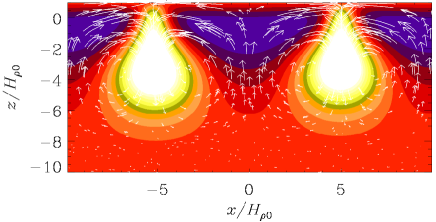
Figure 2: Left: Growth of the rms value of mean velocity and mean magnetic field for two runs with different degree of stratification. Right: Spontaneous production of magnetic flux structures: early evolution of magnetic field in the $y$ direction (color coded) together with velocity vectors in the $xz$ plane. Adapted from Ref. [41].

The instability develops concentrations with a certain horizontal wavelength $\lambda_{\perp}\approx 10\,H_{\rho 0}$ or horizontal wavenumber $k_{\perp}=2\pi/\lambda_{\perp}$; see right panel of figure 2. Here, $H_{\rho 0}$ is the density scale height at some reference depth slightly below the surface. Thus, we have $k_{\perp}H_{\rho 0}\approx 0.6$, which is roughly consistent with subsequent studies [12, 13, 40].

During the nonlinear evolution of NEMPI, the magnetic structures shown in figure 3 take the form of a droplet and look like a balloon hanging upside down filled with water. In earlier papers we referred to the associated downflows as the “potato sack” effect [41, 10]. We discuss this effect in more detail later in Sect. 5.

4 Detection of NEMPI in DNS

Let us now turn to the explicit verification of NEMPI using DNS in strongly stratified forced turbulence. Early attempts to detect NEMPI failed and it was clear only afterwards why no NEMPI developed: the scale separation ratio, $k_{\rm f}/k_{1}$, was only about five [12]. Here, $k_{\rm f}$ is the forcing wavenumber and $k_{1}$ is the smallest wavenumber that fits into the domain. Simulations with $k_{\rm f}/k_{1}=15$ did finally show NEMPI [10], but the effect was still relatively weak and became clearly noticeable only after having averaged along the direction of the imposed mean magnetic field. Nevertheless, as seen in figure 3, there is a clear sign of the typical droplet shape associated with subsequent downward motion.

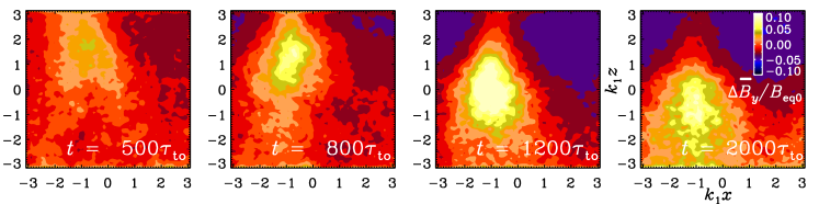
Figure 3: $(\overline{B}_{y}-B_{0})/B_{\rm eq0}$ in the $xz$ plane for magnetic Reynolds number $R_{\rm m}=6$ and imposed field in terms of the equipartition value given by $B_{0}/B_{\rm eq0}=0.05$, showing a descending potato sack structure. Time is in turnover times, $\tau_{\rm to}=(u_{\rm rms}k_{\rm f})^{-1}$ (lower right). Adapted from Ref. [10].

Another reason for not having noticed NEMPI in earlier DNS studies could be related to the fact that the field strength was not in the right range. The understanding of this aspect came as a benefit of having used idealizing condition such as an isothermal equation of state. In that case the scale height is constant and independent of $z$, so the system is similar at all depths except that the density changes. For a given imposed field strength $B_{0}$, there will always be one particular height where $B_{0}/B_{\rm eq}$ takes the preferred value for NEMPI to develop ($B_{0}/B_{\rm eq}$ is in the range $0.03$–$0.2$; see table 1 of Ref. [32]). If the field strength is increased, NEMPI develops simply at a larger depth [42]. This is shown in figure 4.

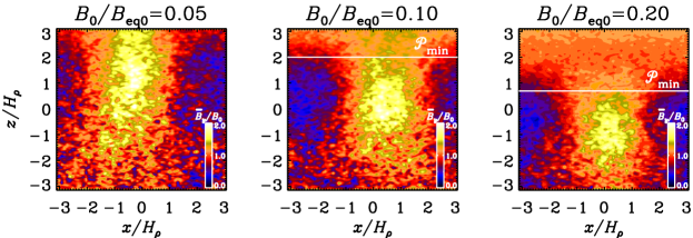
Figure 4: $\overline{B}_{y}/B_{0}$ from DNS for three values of the imposed field strength at the end of the linear growth phase of NEMPI for $R_{\rm m}=18$ and $\mbox{\rm Pr}_{M}=0.5$. The location of the ${\cal P}_{\rm min}$ line is indicated in panels 2 and 3, while for panel 1 it lies above the computational domain. Adapted from Ref. [13].

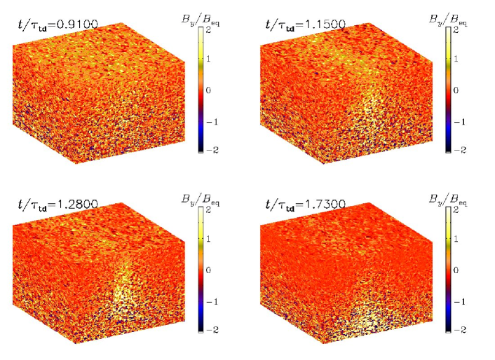
Figure 5: Visualizations of $B_{y}$ on the periphery of the domain for different times. Adapted from Ref. [12].

In figure 5 we show the magnetic field for a run with $k_{\rm f}/k_{1}=30$, so NEMPI is now stronger than before and the flux concentrations can clearly be seen in snapshots even without averaging. Here, time is given in turbulent-diffusive times, $\tau_{\rm td}=(\eta_{\rm t0}k_{1}^{2})^{-1}$, where $\eta_{\rm t0}=u_{\rm rms}/3k_{\rm f}$ is the estimated turbulent magnetic diffusivity. Again, the field concentration develops first near the top of the domain and then sinks downward. Clearly, this is just opposite to the usual magnetic buoyancy instability [43, 44], where magnetic fields rise toward the surface. This underlines the physical reality of a negative effective magnetic pressure.

Figure 6: Visualization of $\overline{B}_{y}(x,z)$ for an elongated box with $R_{\rm m}=36$ at a time during the statistically steady state. The top panel shows the $y$ average $\overline{B}_{y}/B_{\rm eq}$ at one time while the lower panel shows an additional time average $\langle\overline{B}_{y}\rangle_{t}/B_{\rm eq}$ covering about 80 turnover times. The dimensions in the horizontal and vertical directions are $H_{\rho}$ so the extent is $16\pi H_{\rho}\times 2\pi H_{\rho}$. Adapted from Ref. [12].

Making the domain wider results in the replication of statistically similar flux concentrations. In figure 6 we see that the wavelength is approximately $8\,H_{\rho}$, so $k_{\perp}H_{\rho}=2\pi/8\approx 0.8$. Similar behavior is also found in MFS, both in two and three dimensions [40].

In Ref. [13], an expression for the growth rate of NEMPI was derived using the anelastic approximation under the assumption $H_{\rho}={\rm const}{}$ (see for details Sect. 2). Remarkable agreement with the numerical calculations has been reported in Ref. [13], where several examples were shown that demonstrated quantitative agreement between DNS and MFS; see also Ref. [40].

5 NEMPI with vertical field

In the presence of a vertically imposed magnetic field, $\bm{B}_{0}=(0,0,B_{0})$, the appropriate boundary condition is the so-called vertical field boundary condition, $A_{x,z}=A_{y,z}=A_{z}=0$. It turns out that with a vertical field, the effect of NEMPI is much stronger; see figure 7 for a visualization of $B_{z}$ on the periphery of the computational domain at different times. In this case, $\overline{B}_{z}/B_{\rm eq}$ can reach and even exceed unity. One reason for this is that the downflows associated with NEMPI lead to a converging return flow in the upper layers, which pinches the field further. Cross sections of the resulting magnetic field look quite different from standard visualizations of buoyant flux tubes that rise and pierce the surface. Here, the magnetic field seems to diffuse out as one goes deeper down, see figure 8, where the field lines have been computed after taking an axisymmetric average of the magnetic field obtained from the DNS.

Figure 7: Evolution from a uniform initial state toward a circular spot for $B_{z0}/B_{\rm eq0}=0.02$. Here, $B_{z}/B_{\rm eq0}$ is shown on the periphery of the domain. Dark shades correspond to strong vertical fields. Time is in units of $\tau_{\rm td}$. An animation is available on http://youtu.be/Um_7Hs_1RzA. Adapted from Ref. [11].

Figure 8: Cuts of $B_{z}/B_{\rm eq}(z)$ in the $xy$ plane at the top boundary ($z/H_{\rho}=\pi$) and the $xz$ plane through the middle of the spot at $y=0$. In the $xz$ cut, we also show magnetic field lines and flow vectors obtained by numerically averaging in azimuth around the spot axis. Adapted from Ref. [11].

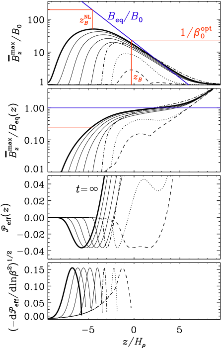
Figure 9: Left: $\overline{B}_{z}/B_{\rm eq}$ together with field lines and flow vectors from an axisymmetric MFS with $B_{0}/B_{\rm eq0}=0.05$. The flow speed varies from $-0.27u_{\rm rms}$ (downward) to $0.08u_{\rm rms}$ (upward). Right: Time evolution of normalized vertical magnetic field profiles, (a) $\overline{B}_{z}^{\rm max}/B_{0}$ together with $B_{\rm eq}(z)/B_{0}$ (shown by blue line), (b) $\overline{B}_{z}^{\rm max}/B_{\rm eq}(z)$, as well as (c) ${\cal P}_{\rm eff}(z)$ and (d) $(-{\rm d}{}{\cal P}_{\rm eff}/{\rm d}{}\ln\beta^{2})^{1/2}$, from a MFS with $B_{0}/B_{\rm eq0}=0.05$ at $t/\tau_{\rm td}=2.9$ (dashed), 3 (dotted), 3.1 (dash-dotted), 3.3, 3.7, 4.2., 5, and 50 (thick solid line). The blue solid lines indicate $B_{\rm eq}(z)$, normalized by (a) $B_{0}$ and (b) by itself (corresponding thus to unity). The red lines indicate the locations $z_{B}$ and $z_{B}^{\rm NL}$ during linear and nonlinear (NL) phases of the evolution, as well as relevant intersections with normalized values of $\overline{B}_{z}^{\rm max}$ and $B_{\rm eq}$. Adapted from Ref. [40].

The resulting flux concentrations from NEMPI with a vertical imposed magnetic field are much stronger compared to the case with a horizontal field because of the apparent absence of the aforementioned potato sack effect for vertical field. This effect has been observed in turbulence with a horizontal imposed magnetic field; see figures 3 and 4. The potato sack effect is a direct consequence of the negative effective magnetic pressure, making such magnetic structures heavier than their surroundings [41, 10, 29]. The potato sack effect removes horizontal magnetic field structures from regions in which NEMPI is excited and pushes them downward. For vertical magnetic field, the heavier fluid moves downward along the field without affecting the flux tube, so that NEMPI is not stabilized prematurely by the potato sack effect.

In a mean-field framework, it is quite straightforward to produce an axisymmetric model of a magnetic spot [40]. However, it is important to make sure that the outer radius of the domain is chosen in a suitable manner. If it is too big, downflows will develop on the rim of the cylinder; see figure 8 of Ref. [40]. Furthermore, for an isothermal gas it is straightforward to extend the domain arbitrarily in the vertical direction upward and downward. Figure 9 shows the resulting flux concentration in a domain tall enough so that the field becomes uniform both far above and far below the flux concentration.

6 Bipolar regions and dynamo-generated magnetic fields

In reality, there will never be a purely vertical nor a purely horizontal imposed field, but a dynamo-generated one which always has some natural horizontal variability. This would allow the field to penetrate the surface. Thus, when allowing for a layer above which there is no turbulence, one can see the development of bipolar regions [45, 46]. This layer is meant to represent the effects of a free surface or a photosphere. An example of this is shown in figure 10. Here, a Cartesian domain of isothermally stratified gas was divided into two layers. In the lower layer, turbulence was forced with transverse nonhelical random waves, whereas in the upper layer no flow was driven. A weak uniform magnetic field was imposed in the entire domain at all times. Formation of bipolar magnetic structures was found over a large range of parameters. The magnetic structures became more intense for higher stratification until a density contrast of around 100 across the turbulent layer was reached. The magnetic field in bipolar regions was found to increase with higher imposed field strength until the field became comparable to the equipartition field strength of the turbulence. A weak imposed horizontal field component turned out to be necessary for generating bipolar structures. In the case of bipolar region formation, an exponential growth of the large-scale magnetic field was found, which is a clear indication of a hydromagnetic instability [46]. Additionally, the flux concentrations were correlated with strong large-scale downward-oriented converging flows. These findings strongly suggest that NEMPI is indeed responsible for magnetic flux concentrations found in this system.

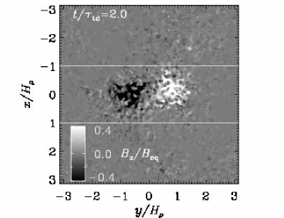
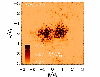
Figure 10: Left panel: normalized vertical magnetic field $B_{z}/B_{\rm eq}$ of the bipolar region at the surface ($z=0$) of the simulation domain. Right panel: normalized magnetic energy ${\overline{\bm{B}}}^{2}/B_{\rm eq}^{2}$ of the two regions relative to the rest of the surface. Note that we clip both color tables to increase the contrast of the structure. The field strength reaches around $B_{z}/B_{\rm eq}=1.4$. Adapted from Ref. [45].

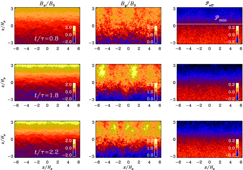
Figure 11: Visualization of $\overline{B}_{x}/B_{0}$ and $\overline{B}_{y}/B_{0}$ together with effective magnetic pressure for different times. Here the angular velocity is $\Omega=0.15$, corresponding to a Coriolis number $\mbox{\rm Co}=0.09$. Adapted from Ref. [34].

Many subsequent studies of NEMPI have been undertaken in the meantime. Of particular interest is the case where the main field is not an imposed one, but the result of a dynamo. This situation was first studied in MFS in spherical shells [47], and later also in Cartesian domains [34]. An example is shown in figure 11. Here, the large-scale dynamo is the result of the combined action of stratification and rotation giving rise to kinetic helicity of the turbulence. On the other hand, if rotation is too strong, NEMPI will be suppressed [48, 49].

The suppression of NEMPI by rotation came as a surprise, especially because the critical values of the maximum permissible rotation speed were found to be rather low. In dynamo theory the importance of rotation on the flow is usually measured in terms of the Coriolis number, $\mbox{\rm Co}=2\Omega\tau_{\rm td}$, but those values are only around 0.1 when NEMPI begins to be suppressed; see figure 2 of [49]. They argued that the reason for this is the fact that the growth time for NEMPI is longer than the turnover time of the turbulence $\tau_{\rm td}$. If one normalizes instead with the typical growth rate of NEMPI, $\lambda_{0*}$ the critical values of $2\Omega/\lambda_{0*}$ are found to be slightly above unity.

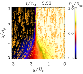
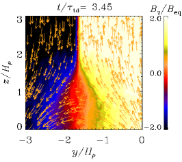
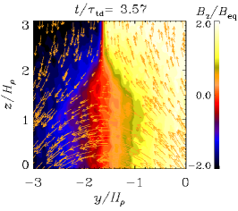
Figure 12: Time evolution of $\overline{B}_{z}/B_{\rm eq}$, together with $\overline{B}_{y}/B_{\rm eq}$ and $\overline{B}_{z}/B_{\rm eq}$ vectors for a case where the magnetic field is generated by a helical dynamo. Adapted from Ref. [35]. Reproduced from S. Jabbari et al. Turbulent Reconnection of Magnetic Bipoles in Stratified Turbulence. MNRAS (2016) 459 (4): 4046-4056. Published by Oxford University Press on behalf of the Royal Astronomical Society online at: http://mnras.oxfordjournals.org/content/459/4/4046.abstract?sid=5ba53a74-4653-4fbc-bc7d-58b9a4ffb816

Although NEMPI does not appear to be excited when rotation is too strong, simulations show that magnetic flux concentrations are still being produced when there is strong stratification and a dynamo is operating preferentially in the deeper parts [34]. In figure 12 we show a case where a sub-equipartition strength magnetic field is produced in the deeper parts and leads to a super-equipartition strength magnetic fields in the surface layers. The different polarities can then be driven together to form sharp structures in the form of an inverted Y-shaped pattern in a vertical cross-section [35, 50]. This is an example where the phenomenon of turbulent magnetic reconnection has been seen to occur in a natural setting. Similar behavior has also been seen in global spherical shell dynamos [51]. In simulations [35, 50], the generated magnetic field reached super-equipartition levels so rapidly that it was not possible to detect NEMPI during the growth of the magnetic field. It should be noted that NEMPI cannot be excited for super-equipartition magnetic fields.

To investigate the role of magnetic reconnection, the flow around the sharp interface was zoomed in, and the dynamics of the current sheet in this region was studied [35]. The reconnection rate was determined independently through the inflow velocity in the vicinity of the current sheet and via the electric field in the reconnection region. For large Lundquist numbers ($\mbox{\rm Lu}>1000$), the reconnection rate was found to be nearly independent of the value of Lu [35], where $\mbox{\rm Lu}=v_{\rm A}L_{c}/\eta$ with $L_{c}$ being the length of the current sheet. This agrees with earlier studies of turbulent reconnection [52], which also showed independence of Ohmic resistivity [53, 54], as well as results of recent numerical simulations performed by other groups in simpler settings [52, 55, 56, 57, 58].

7 Turbulent convection

In view of application to the Sun as a next step, it will be important to consider more realistic modeling and include the effects of convectively-driven turbulence. It is not obvious that NEMPI applies straightforwardly to this case. It was shown already early on that—even in convection—the relevant NEMPI parameter $q_{\rm p}$ is indeed much larger than unity [29], favoring the possibility of NEMPI. Subsequent convection simulations with an imposed magnetic field [30] yielded structures that are strongly reminiscent of those found in realistic solar surface simulations in the presence of full radiative transport [27].

The spontaneous formation of surface magnetic structures from a large-scale $\alpha^{2}$ dynamo by strongly stratified thermal convection in Cartesian geometry has recently also been studied by [31]. They found that large-scale magnetic structures are formed at the surface only in cases with strong stratification. The presence of rapid uniform rotation was an argument in [31] that NEMPI seems not to be responsible for these structures. On the other hand, the combined effect of rapid uniform rotation and stratification can produce helicity and an $\alpha$ effect, which causes a large-scale $\alpha^{2}$ dynamo. A similar situation was encountered in connection with the dynamo simulations of forced turbulence, where rotation also did not suppress the formation of structures [35]. Thus, the question of the origin of these structures remains unsettled.

The direct detection of negative effective magnetic pressure in turbulent convection with dynamo-generated magnetic fields is a difficult problem. In many existing convection simulations, unlike the case of forced turbulence, the scale separation between the integral scale of the turbulence and the size of the domain is not large enough for the excitation of NEMPI and the formation of sharp magnetic structures.

8 Cross helicity effect

The role of NEMPI is not always evident, especially when the magnetic field strongly exceeds the equipartition value. However, all these simulations have in common that there is a vertical magnetic field such that $\bm{g}\cdot{\overline{\bm{B}}}\neq 0$. Interestingly, $\bm{g}\cdot{\overline{\bm{B}}}$ is not only a pseudoscalar, but it is odd in the magnetic field. In MHD, there is an important invariant of the ideal equations, namely the cross helicity $\langle\bm{u}\cdot\bm{B}\rangle$ [59]. It is often not important unless it was present in the initial conditions. However, it is not too surprising that $\langle\bm{u}\cdot\bm{B}\rangle$ is generated whenever $\bm{g}\cdot{\overline{\bm{B}}}$ is nonzero. This was explored in Ref, [3], where it was found that

$$\langle\bm{u}\cdot\bm{b}\rangle={\eta_{\rm t}\over c_{\rm s}^{2}}\,\bm{g}\cdot{\overline{\bm{B}}}=-{\eta_{\rm t}\over H_{\rho}}\overline{B}_{z}.$$ (37)

If the turbulence intensity is nonuniform, there is yet another contribution to $\langle\bm{u}\cdot\bm{b}\rangle$ that is proportional to $\eta_{\rm t}({\bm{\nabla}}\ln u_{\rm rms})\cdot{\overline{\bm{B}}}$, which was first obtained in Ref. [60].

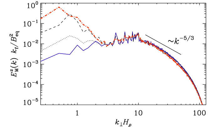
Figure 13: Normalized spectra of $B_{z}$ from DNS at normalized times $t\eta_{\rm t0}/H_{\rho}^{2}\approx 0.2$ (solid blue), 0.5 (dotted), 1 (dashed), and 2.7 (dash-dotted red) with $k_{\rm f}H_{\rho}=10$ and $k_{1}H_{\rho}=0.25$. Adapted from Ref. [40].

All the simulations that produce large-scale magnetic field structures display what can be characterized as inverse cascade or inverse transfer behavior of magnetic field from the driving scale to large scales with a horizontal wavenumber $k_{\perp}$ such that $k_{\perp}H_{\rho}\approx 0.8$ or even less. The role of the conservation property of $\langle\bm{u}\cdot\bm{B}\rangle$ still needs to be explored, but it is clear that there is a remarkable analogy between inverse transfer seen in figure 13 and that of a large-scale dynamo, where the conservation of magnetic helicity is known to lead to an inverse cascade [61, 62, 63].

9 Concluding remarks

The purpose of this review has been to highlight the fact that the presence of gravitational stratification introduces a qualitatively new phenomenon in MHD turbulence, namely the formation of large-scale magnetic structures via excitation of NEMPI. Turbulence causes a modification of the large-scale magnetic pressure, so that the effective magnetic pressure becomes negative for large fluid and magnetic Reynolds numbers, and this results in the excitation of NEMPI. DNS demonstrate that the effective magnetic pressure can be negative in any kind of turbulence, e.g., in non-stratified and stratified isothermal turbulence, polytropic stably stratified turbulence, turbulent convection, and in turbulence with an upper non-turbulent layer. However, the actual instability is excited only in stratified turbulence when the initial mean magnetic field is less than the equipartition field. For very large fluid and magnetic Reynolds numbers, NEMPI weakly dependent on the level of turbulence. In some cases, where there is locally a vertical magnetic field, NEMPI causes the formation of magnetic spots.

In astrophysics, there are many examples where MHD turbulence is accompanied by strong density stratification. A prediction from our studies reviewed in this paper would be that such systems should exhibit magnetic spots. We do not know whether there is a direct relation to sunspots, which are generally hypothesized as being the result of deeply rooted thin magnetic flux tubes. Whether such isolated flux tubes really exist and how they are formed is an open question.

We do know of magnetic flux tubes in MHD turbulence [64, 65], that are analogous to vortex tubes in hydrodynamic turbulence [66], but these tend to scale with the resistive scale [67], so such tubes would become smaller as the magnetic Reynolds number is increased. Global simulations of convective spherical shell dynamos have been used to visualize magnetic flux tubes [68, 69]. Those may well be the type of tubes seen in earlier Cartesian simulations, but they could also be local field enhancements resulting from the large-scale dynamo. It is hard to imagine that these flux structures alone can explain the formation of sunspots, unless there was some kind of reamplification. Clearly, as future simulations of global dynamos gain in resolution, they would eventually display spots, just like the Sun and other stars do. It will then be important to have possible frameworks in place for understanding such spots. We hope that the present review has provided some relevant inspiration beyond the standard paradigm.

Further steps toward more realistic modeling of the formation of magnetic spots and bipolar regions include replacing forced turbulence by self-consistently driven convective motions that are influenced by the radiative cooling at the surface together with partial ionization. Including more realistic physical processes at the solar surface might also help to reproduce the surrounding spot structures.

Acknowledgments

IR and NK thank NORDITA for hospitality and support during their visits. This work has been supported in parts by the Swedish Research Council grant No. 621-2011-5076 and the Research Council of Norway under the FRINATEK grant No. 231444.

References

$Header: /var/cvs/brandenb/tex/nathan_igor/NEMPI/paper.tex,v 1.98 2016/12/24 14:34:04 brandenb Exp $

References

- [1] Iroshnikov, R. S. 1964 Turbulence of a conducting fluid in a strong magnetic field. Sov. Astron. 7, 566–571.
- [2] Kraichnan, R. H. 1965 Inertial-range spectrum of hydromagnetic turbulence. Phys. Fluids 8, 1385–1387.
- [3] Rüdiger, G., Kitchatinov, L. L., & Brandenburg, A. 2011 Cross helicity and turbulent magnetic diffusivity in the solar convection zone. Solar Phys. 269, 3–12.
- [4] Kleeorin, N. I., Rogachevskii, I. V., & Ruzmaikin, A. A. 1989 Negative magnetic pressure as a trigger of large-scale magnetic instability in the solar convective zone. Pis. Astron. Zh. 15, 639–645.
- [5] Kleeorin, N. I., Rogachevskii, I. V., Ruzmaikin, A. A. 1990 Magnetic force reversal and instability in a plasma with advanced magnetohydrodynamic turbulence. Sov. Phys. JETP 70, 878–883.
- [6] Kleeorin, N., Mond, M., & Rogachevskii, I. 1993 Magnetohydrodynamic instabilities in developed small-scale turbulence. Phys. Fluids 5, 4128–4134.
- [7] Kleeorin, N., & Rogachevskii, I. 1994 Effective Ampère force in developed magnetohydrodynamic turbulence. Phys. Rev. E 50, 2716–2730.
- [8] Kleeorin, N., Mond, M., & Rogachevskii, I. 1996 Magnetohydrodynamic turbulence in the solar convective zone as a source of oscillations and sunspots formation. Astron. Astrophys. 307, 293–309.
- [9] Rogachevskii, I., & Kleeorin, N. 2007 Magnetic fluctuations and formation of large-scale inhomogeneous magnetic structures in a turbulent convection. Phys. Rev. E 76, 056307.
- [10] Brandenburg, A., Kemel, K., Kleeorin, N., Mitra, D., & Rogachevskii, I. 2011 Detection of negative effective magnetic pressure instability in turbulence simulations. Astrophys. J. Letters 740, L50.
- [11] Brandenburg, A., Kleeorin, N., & Rogachevskii, I. 2013 Self-assembly of shallow magnetic spots through strongly stratified turbulence. Astrophys. J. Letters 776, L23.
- [12] Kemel, K., Brandenburg, A., Kleeorin, N., Mitra, D., & Rogachevskii, I. 2012 Spontaneous formation of magnetic flux concentrations in stratified turbulence. Solar Phys. 280, 321–333.
- [13] Kemel, K., Brandenburg, A., Kleeorin, N., Mitra, D., & Rogachevskii, I. 2013 Active region formation through the negative effective magnetic pressure instability. Solar Phys. 287, 293–313.
- [14] Kemel, K., Brandenburg, A., Kleeorin, N., & Rogachevskii, I. 2013 Nonuniformity effects in the negative effective magnetic pressure instability. Phys. Scr. T155, 014027.
- [15] Galloway, D. J., Proctor, M. R. E. & Weiss, N. O. 1977 Formation of intense magnetic fields near the surface of the Sun. Nature 266, 686–689.
- [16] Tao, L., Weiss, N. O., Brownjohn, D. P., & Proctor, M. R. E. 1998 Flux separation in stellar magnetoconvection. Astrophys. J. 496, L39–L42.
- [17] Caligari, P., Moreno-Insertis, F., & Schüssler, M. 1995 Emerging flux tubes in the solar convection zone. 1. Asymmetry, tilt, and emergence latitude. Astrophys. J. 441, 886–902.
- [18] Fan, Y. 2009 Magnetic Fields in the Solar Convection Zone. Liv. Rev. Solar Phys. 6, 4.
- [19] Charbonneau, P. 2010 Dynamo Models of the Solar Cycle. Liv. Rev. Solar Phys. 7, 3.
- [20] Birch, A. C., Braun, D. C., & Fan, Y. 2010 An estimate of the detectability of rising flux tubes. Astrophys. J. 723, L190–L194.
- [21] Birch, A. C., Schunker, H., Braun, D. C., Cameron, R., Gizon, L., Löptien, B., & Rempel, M. 2016 A low upper limit on the subsurface rise speed of solar active regions. Sci. Adv. 2, e1600557.
- [22] Singh, N. K., Raichur, H., & Brandenburg, A. 2016 High-wavenumber solar -mode strengthening prior to active region formation. Astrophys. J. 832, 120.
- [23] Clark, Jr., A. 1965 Some exact solutions in magnetohydrodynamics with astrophysical applications. Phys. Fluids 8, 644–657.
- [24] Weiss, N. O. 1966 The expulsion of magnetic flux by eddies. Proc. Roy. Soc. Lond. 293, 310–328.
- [25] Kitiashvili, I. N., Kosovichev, A. G., Wray, A. A., & Mansour, N. N. 2010 Mechanism of spontaneous formation of stable magnetic structures on the Sun. Astrophys. J. 719, 307–312.
- [26] Tian, C. & Petrovay, K. 2013 Structures in compressible magnetoconvection and the nature of umbral dots. Astron. Astrophys. 551, A92.
- [27] Stein, R. F., & Nordlund, Å. 2012 On the formation of active regions. Astrophys. J. Letters 753, L13.
- [28] Rempel, M., & Schlichenmaier, R. 2011 Sunspot modeling: From simplified models to radiative MHD simulations. Liv. Rev. Sol. Phys. 8, 3.
- [29] Käpylä, P. J., Brandenburg, A., Kleeorin, N., Mantere, M. J., & Rogachevskii, I. 2012 Negative effective magnetic pressure in turbulent convection. Monthly Notices Roy. Astron. Soc. 422, 2465–2473.
- [30] Käpylä, P. J., Brandenburg, A., Kleeorin, N., Käpylä, M. J., & Rogachevskii, I. 2016 Magnetic flux concentrations from turbulent stratified convection. Astron. Astrophys. 588, A150.
- [31] Masada, Y., & Sano, T. 2016 Spontaneous formation of surface magnetic structure from large-scale dynamo in strongly stratified convection. Astrophys. J. 822, L22.
- [32] Losada, I. R., Brandenburg, A., Kleeorin, N., & Rogachevskii, I. 2014 Magnetic flux concentrations in a polytropic atmosphere. Astron. Astrophys. 564, A2.
- [33] Mitra, D., Brandenburg, A., Kleeorin, N., Rogachevskii, I. 2014 Intense bipolar structures from stratified helical dynamos. Monthly Notices Roy. Astron. Soc. 445, 761–769.
- [34] Jabbari, S., Brandenburg, A., Losada, I. R., Kleeorin, N., & Rogachevskii, I. 2014 Magnetic flux concentrations from dynamo-generated fields. Astron. Astrophys. 568, A112.
- [35] Jabbari, S., Brandenburg, A., Mitra, D., Kleeorin, N., & Rogachevskii, I. 2016 Turbulent reconnection of magnetic bipoles in stratified turbulence. Monthly Notices Roy. Astron. Soc. 459, 4046–4056.
- [36] Landau, L. D., & Lifshitz, E. M. 1975 Classical Theory of Fields (Oxford: Pergamon).
- [37] Landau, L. D., & Lifshitz, E. M. 1984 Theory of Elasticity (Oxford: Pergamon).
- [38] Brandenburg, A., Kemel, K., Kleeorin, N., & Rogachevskii, I. 2012 The negative effective magnetic pressure in stratified forced turbulence. Astrophys. J. 749, 179.
- [39] Rüdiger, G., Kitchatinov, L. L., & Schultz, M. 2012 Suppression of the large-scale Lorentz force by turbulence. Astron. Nachr. 333, 84–91.
- [40] Brandenburg, A., Gressel, O., Jabbari S., Kleeorin, N. & Rogachevskii, I. 2014 Mean-field and direct numerical simulations of magnetic flux concentrations from vertical field. Astron. Astrophys. 562, A53.
- [41] Brandenburg, A., Kleeorin, N., & Rogachevskii, I. 2010 Large-scale magnetic flux concentrations from turbulent stresses. Astron. Nachr. 331, 5–13.
- [42] Kemel, K., Brandenburg, A., Kleeorin, N., & Rogachevskii, I. 2012 Properties of the negative effective magnetic pressure instability. Astron. Nachr. 333, 95–100.
- [43] Parker, E. N. 1967 The dynamical state of the interstellar gas and field. 3. Turbulence and enhanced diffusion. Astrophys. J. 149, 535–535.
- [44] Hughes, D. W., Proctor, M. R. E. 1988 Magnetic fields in the solar convection zone: Magnetoconvection and magnetic buoyancy. Ann. Rev. Fluid Dyn. 20, 187–223.
- [45] Warnecke, J., Losada, I. R., Brandenburg, A., Kleeorin, N., & Rogachevskii, I. 2013 Bipolar magnetic structures driven by stratified turbulence with a coronal envelope. Astrophys. J. Letters 777, L37.
- [46] Warnecke, J., Losada, I. R., Brandenburg, A., Kleeorin, N., & Rogachevskii, I. 2016 Bipolar region formation in stratified two-layer turbulence. Astron. Astrophys. 589, A125.
- [47] Jabbari, S., Brandenburg, A., Kleeorin, N., Mitra, D., & Rogachevskii, I. 2013 Surface flux concentrations in a spherical dynamo. Astron. Astrophys. 556, A106.
- [48] Losada, I. R., Brandenburg, A., Kleeorin, N., Mitra, D., & Rogachevskii, I. 2012 Rotational effects on the negative magnetic pressure instability. Astron. Astrophys. 548, A49.
- [49] Losada, I. R., Brandenburg, A., Kleeorin, N., & Rogachevskii, I. 2013 Competition of rotation and stratification in flux concentrations. Astron. Astrophys. 556, A83.
- [50] Jabbari, S., Brandenburg, A., Kleeorin, N., & Rogachevskii, I. 2016 “Sharp magnetic structures from dynamos with density stratification,” Monthly Notices Roy. Astron. Soc. (submitted). 1607.08897
- [51] Jabbari, S., Brandenburg, A., Kleeorin, N., Mitra, D., & Rogachevskii, I. 2015 Bipolar magnetic spots from dynamos in stratified spherical shell turbulence. Astrophys. J. 805, 166.
- [52] Loureiro, N. F., Uzdensky, D. A., Schekochihin, A. A., Cowley, S. C., & Yousef, T. A. 2009 Turbulent magnetic reconnection in two dimensions. Astrophys. J. 399, L146.
- [53] Lazarian, A., & Vishniac E. T. 1999 Reconnection in a weakly stochastic field. Astrophys. J. 517, 700.
- [54] Lazarian, A., Kowal, G., Takamoto, M., de Gouveia Dal Pino, E. M., & Cho, J. 2016 Theory and applications of non-relativistic and relativistic turbulent reconnection. In.: Magnetic Reconnection, Astrophysics and Space Science Library, Springer, 427, 409.
- [55] Kowal, G., Lazarian, A., Vishniac E. T., & Otmianowska-Mazur, K. 2009 Numerical Tests of Fast Reconnection in Weakly Stochastic Magnetic Fields. Astrophys. J. 700, 63.
- [56] Huang, Y.-M. & Bhattacharjee, A. 2010 Scaling laws of resistive magnetohydrodynamic reconnection in the high-Lundquist-number, plasmoidunstable regime. Phys. Plasmas 17, 062104.
- [57] Loureiro, N. F., Samtaney, R., Schekochihin, A. A. & Uzdensky, D. A. 2012 Magnetic reconnection and stochastic plasmoid chains in high-Lundquist-number plasmas. Phys. Plasmas 19, 042303.
- [58] Beresnyak, A. 2013 On the rate of spontaneous magnetic reconnection, arXiv: 1301.7424.
- [59] Woltjer, L. 1958 A theorem on force-free magnetic fields. Proc. Natl. Acad. Sci. 44, 489–491.
- [60] Kleeorin, N., Kuzanyan, K., Moss, D., Rogachevskii, I., Sokoloff, D., & Zhang, H. 2003 Magnetic helicity evolution during the solar activity cycle: observations and dynamo theory. Astron. Astrophys. 409, 1097–1105.
- [61] Frisch, U., Pouquet, A., Léorat, J., & Mazure, A. 1975 Possibility of an inverse cascade of magnetic helicity in hydrodynamic turbulence. J. Fluid Mech. 68, 769–778.
- [62] Pouquet, A., Frisch, U., & Léorat, J. 1976 Strong MHD helical turbulence and the nonlinear dynamo effect. J. Fluid Mech. 77, 321–354.
- [63] Brandenburg, A. 2001 The inverse cascade and nonlinear alpha-effect in simulations of isotropic helical hydromagnetic turbulence. Astrophys. J. 550, 824–840.
- [64] Nordlund, Å., Brandenburg, A., Jennings, R. L., Rieutord, M., Ruokolainen, J., Stein, R. F., & Tuominen, I. 1992 Dynamo action in stratified convection with overshoot. Astrophys. J. 392, 647–652.
- [65] Brandenburg, A., Jennings, R. L., Nordlund, Å., Rieutord, M., Stein, R. F., & Tuominen, I. 1996 Magnetic structures in a dynamo simulation. J. Fluid Mech. 306, 325–352.
- [66] She, Z.-S., Jackson, E., & Orszag, S. A. 1990 Intermittent vortex structures in homogeneous isotropic turbulence. Nature 344, 226–228.
- [67] Brandenburg, A., Procaccia, I., & Segel, D. 1995 The size and dynamics of magnetic flux structures in MHD turbulence. Phys. Plasmas 2, 1148–1156.
- [68] Nelson, N. J., Brown, B. P., Brun, A. S., Miesch, M. S., & Toomre, J. 2013 Magnetic wreaths and cycles in convective dynamos. Astrophys. J. 762, 73.
- [69] Nelson, N. J., Brown, B. P., Brun, A. S., Miesch, M. S., & Toomre, J. 2014 Buoyant magnetic loops generated by global convective dynamo action. Solar Phys. 289, 441–458.