Differential Inequalities in Multi-Agent Coordination and Opinion Dynamics Modeling.

Abstract

Many distributed algorithms for multi-agent coordination employ the simple averaging dynamics, referred to as the Laplacian flow. Besides the standard consensus protocols, examples include, but are not limited to, algorithms for aggregation and containment control, target surrounding, distributed optimization and models of opinion formation in social groups. In spite of their similarities, each of these algorithms has been studied using separate mathematical techniques. In this paper, we show that stability and convergence of many coordination algorithms involving the Laplacian flow dynamics follow from the general consensus dichotomy property of a special differential inequality. The consensus dichotomy implies that any solution to the differential inequality is either unbounded or converges to a consensus equilibrium. In this paper, we establish the dichotomy criteria for differential inequalities and illustrate their applications to multi-agent coordination and opinion dynamics modeling.

1 Introduction

Distributed algorithms for multi-agent coordination have various applications to science and engineering, including control of robotic formations, scheduling of sensor networks, optimization and filtering, modeling biological and social systems. The relevant results are discussed in the works (Ren and Beard, 2008; Mesbahi and Egerstedt, 2010; Ren and Cao, 2011; Savkin et al., 2015; Proskurnikov and Cao, 2016a; Bullo, 2016; Proskurnikov and Tempo, 2017) and references therein. A “benchmark” problem in multi-agent control is to establish consensus (that is, agreement on some quantity of interest) among the agents interacting over a general graph. A simple consensus algorithm, originated from some opinion formation models (Proskurnikov and Tempo, 2017), is called the Laplacian flow (Bullo, 2016). Being a counterpart (Ferrari-Trecate et al., 2006) of the well-known heat equation, which is used in physics to describe diffusion processes, this algorithm employs the Laplacian matrix $L(t)$ of the interaction graph

$$\dot{x}(t)=-L(t)x(t).$$ (1)

The state vector’s $i$th component $x_{i}(t)$ stands for some value, owned by agent $i$ and representing some quantity of interest (e.g. temperature or altitude). The Laplacian flow dynamics (1) describe the agents’ interactions in order to agree on this quantity, which means that all $x_{i}(t)$ converge to a common value. Numerous extensions of the protocol (1) have been studied in the literature (Ren and Beard, 2008; Ren and Cao, 2011; Cao et al., 2013).

The effect of the interaction graph on establishing consensus has been studied up to a certain exhaustiveness by using the results on convergence of products of stochastic matrices (Cao et al., 2008; Ren and Beard, 2008) and special Lyapunov functions (Moreau, 2004; Lin et al., 2007; Münz et al., 2011). Consensus is established under rather mild assumption of “repeated” (“uniform”) connectivity of the graph; this condition can be further relaxed for some special types of graphs (Hendrickx and Tsitsiklis, 2013). The algorithms (1) have inspired numerous protocols for synchronization of general dynamical systems (Ren and Cao, 2011; Cao et al., 2013).

In spite of the progress in the analysis of consensus algorithms, the relevant mathematical techniques are not directly applicable to other distributed coordination algorithms, employing the idea of the Laplacian flows. The algorithms for containment and aggregation control (Ren and Cao, 2011; Shi and Hong, 2009), target surrounding (Lou and Hong, 2015) and convex optimization (Shi et al., 2013), as well as some models of opinion dynamics (Altafini, 2013) are similar in spirit to consensus protocols; however, each of the mentioned algorithms has been examined by using separate mathematical techniques. It appears, however, that the mentioned algorithms can be analyzed in a unified way, since they reduce to the following differential inequalities, associated to the Laplacian flow dynamics (1)

$$\dot{x}(t)\leq-L(t)x(t).$$ (2)

The one-sided inequalities (2) may seem very “loose” restrictions on the solutions $x(t)$. Nevertheless, under natural connectivity assumptions any solution, which is semi-bounded from below, converges to a consensus equilibrium. In particular, the solutions of the differential inequality split into two groups: unbounded solutions and converging ones. For ordinary differential equations the corresponding property is often referred to as the equation’s dichotomy (Yakubovich, 1988). In this paper, we establish the dichotomy properties of the differential inequalities (2) and demonstrate their applications to the problems of multi-agent coordination, distributed optimization algorithms and some models of opinion formation. Some results have been reported in the conference paper (Proskurnikov and Cao, 2016b).

The paper is organized as follows. Section 2 introduces some preliminary concepts and notation. Section 3 introduces the Laplacian differential inequalities and presents their dichotomy conditions. Section 4 illustrates applications of the main results, whose proofs are given in Section 5. Section 6 concludes the paper.

2 Preliminaries and notation

We use $\mathds{1}_{N}$ to denote the column vector of ones $\mathds{1}_{N}\stackrel{{\scriptstyle\Delta}}{{=}}(1,1,\ldots,1)^{\top}\in\mathbb{R}^{N}$. For two vectors $x,y\in\mathbb{R}^{N}$ we write $x\leq y$ (or $y\geq x$) if $x_{i}\leq y_{i}\,\forall i$. Given a vector $x\in\mathbb{R}^{N}$, $|x|\stackrel{{\scriptstyle\Delta}}{{=}}\sqrt{x^{\top}x}$ denotes its Euclidean norm. Given a complex number $z\in\mathbb{C}$, $z^{*}$ denotes its complex conjugate.

Given a closed convex set $\Omega\subset\mathbb{R}^{d}$, the projection operator $P_{\Omega}:\xi\in\mathbb{R}^{d}\mapsto P_{\Omega}(\xi)\in\Omega$ is defined. Denoting $\xi^{p}\stackrel{{\scriptstyle\Delta}}{{=}}\xi-P_{\Omega}(\xi)$, the distance from $\xi$ to $\Omega$ is given by $d_{\Omega}(\xi)\stackrel{{\scriptstyle\Delta}}{{=}}|\xi^{p}|=\min_{\omega\in\Omega}|\xi-\omega|$. For an arbitrary $\omega\in\Omega$, one has $|\xi-P_{\Omega}(\xi)-\alpha(\omega-\xi)|\geq|\xi^{p}|$ for any $\alpha\in[0;1]$, entailing that $(\omega-P_{\Omega}(\xi))^{\top}\xi^{p}\leq 0$, that is, $\measuredangle(\omega-P_{\Omega}(\xi),\xi-P_{\Omega}(\xi))\geq\pi/2$ (Fig. 1). Therefore

$$(\omega-\xi)^{\top}\xi^{p}\leq-|\xi^{p}|^{2}\quad\forall\xi\in\mathbb{R}^{d},\omega\in\Omega$$ (3)

$$\begin{aligned} (\xi_{2}-\xi_{1})^{\top}\xi_{1}^{p}&=(\xi_{2}^{p})^{\top}\xi_{1}^{p}+(P_{\Omega}(\xi_{2})-\xi_{1})^{\top}\xi_{1}^{p}\overset{\eqref{eq.projection1}}{\leq}\\ &\leq(\xi_{2}^{p})^{\top}\xi_{1}^{p}-|\xi_{1}^{p}|^{2}\quad\forall\xi_{1},\xi_{2}\in\mathbb{R}^{d},\end{aligned}$$ (4)

$$(\xi_{2}-\xi_{1})^{\top}(\xi_{2}^{p}-\xi_{1}^{p})\overset{\eqref{eq.projection}}{\geq}|\xi_{2}^{p}-\xi_{1}^{p}|^{2}\quad\forall\xi_{1},\xi_{2}\in\mathbb{R}^{d}.$$ (5)

The inequality (5) implies that the mapping $\xi\mapsto\xi^{p}$ is non-expansive $|\xi_{2}-\xi_{1}|\geq|\xi_{2}^{p}-\xi_{1}^{p}|$. Furthermore, as shown in (Shi and Hong, 2009, Lemma 2), the function $\xi\mapsto d_{\Omega}(\xi)^{2}=|\xi^{p}|^{2}$ is $C^{1}$-smooth with the gradient

$$\nabla\left(d_{\Omega}(\xi)^{2}\right)=2\xi^{p}=2\left(\xi-P_{\Omega}(\xi)\right).$$ (6)

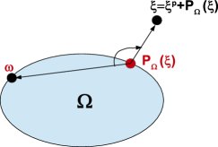
Figure 1: The projection onto a closed convex set

We assume that the reader is familiar with the standard concepts of graph theory, related to directed graphs, such as walks, strong connectivity and strongly connected components, see e.g. (Harary et al., 1965; Bullo, 2016). Henceforth each graph is directed and weighted, being thus a triple $G=(V,E,A)$, where $V$ stands for the set of nodes, $E\subset V\times V$ is a set of arcs and $A=(a_{ij})_{i,j\in V}$ is an adjacency matrix: $a_{ij}>0$ if $(j,i)\in E$ and $a_{ij}=0$ otherwise. By default, the adjacency matrix is assumed to be binary ($a_{ij}\in\{0,1\}$), such a graph is denoted simply by $G=(V,E)$. Any non-negative square matrix $A\in\mathbb{R}^{N\times N}$ can be associated to the graph $G[A]\stackrel{{\scriptstyle\Delta}}{{=}}(V_{N},E[A],A)$, where $V_{N}\stackrel{{\scriptstyle\Delta}}{{=}}\{1,\ldots,N\}$ and $E[A]\stackrel{{\scriptstyle\Delta}}{{=}}\{(j,i):a_{ij}>0\}$. The Laplacian matrix of this graph is defined as follows

$$L[A]=(l_{ij})_{i,j=1}^{N},\quad l_{ij}\stackrel{{\scriptstyle\Delta}}{{=}}\begin{cases}-a_{ij},\;\;i\neq j\\ \sum\limits_{j\neq i}a_{ij},i=j.\end{cases}$$ (7)

A graph is quasi-strongly connected (QSC) if a “root” node exist, from which all other nodes are reachable via walks, or, equivalently, the graph has a directed spanning tree (Ren and Beard, 2008). Given an adjacency matrix $A=(a_{ij})$ and $\delta>0$, define its “truncation” $A^{\delta}=(a_{ij}^{\delta})$ as follows: $a_{ij}^{\delta}=a_{ij}$ if $a_{ij}\geq\delta$ and otherwise $a_{ij}^{\delta}=0$. The graph $G[A]$ is strongly (quasi-strongly) $\delta$-connected if its subgraph $G[A^{\delta}]$, obtained by removing “light-weight” arcs, is strongly (respectively, quasi-strongly) connected.

3 Dichotomies of Differential Inequalities

The proofs of all theorems from this section can be found in Section 5. Henceforth we assume that a time-varying graph $G(t)=(V_{N},E(t),A(t))$ without self-loops ($a_{ii}(t)=0\,\forall i$) is given, which corresponds to the Laplacian $L(t)$. We are interested in the solutions of the differential inequality (2). The function $x:[0;\infty)\to\mathbb{R}^{N}$ is said to be a solution to the inequality (2) if it is absolutely continuous and satisfies (2) for almost any $t\geq 0$.

Throughout this section we also adopt the following assumption, which usually holds in practice and simplifies the further analysis; in some of the subsequent results it can be relaxed.

Assumption 1.

The functions $a_{ij}(t)$ are bounded.

Under Assumption 1, for any $x(0)$ the solution to the equation (1) exists that satisfies (2) and is bounded. The inequality (2) has also many unbounded solutions, e.g. the function $x(t)\stackrel{{\scriptstyle\Delta}}{{=}}x(0)-tc\mathds{1}_{N}$ satisfies (2) for large $c>0$ since $L(t)$ is bounded and $L(t)\mathds{1}_{N}=0$. At the same time, any solution to (2) is upper-semibounded.

Lemma 2.

For any solution $x(t)$ of (2), the function $M(t)\stackrel{{\scriptstyle\Delta}}{{=}}\max\limits_{j}x_{j}(t)$ is non-increasing, so $M(t)\leq M(0)$.

Whereas the class of unbounded solutions of (2) is very broad, under some assumptions on the graph all its bounded solutions have simple asymptotic properties, analogous to the solutions of (1), namely, each bounded solution converges to a consensus equilibrium point $c\mathds{1}_{N}$. In other words, any solution to the inequality (2) is either convergent or unbounded. In this paper, we disclose conditions, ensuring such a dichotomic behavior.

Definition 3.

The differential inequality (2) is called dichotomic, if any of its bounded solutions $x(t)$ has a limit $x^{0}\stackrel{{\scriptstyle\Delta}}{{=}}\lim_{t\to\infty}x(t)$; it is called consensus dichotomic, if all limits $x^{0}$ are consensus equilibria $x^{0}=c^{0}\mathds{1}_{N}$, $c^{0}\in\mathbb{R}$.

Remark 4.

If $x(t)\xrightarrow[t\to\infty]{}c\mathds{1}_{N}$ and $x(t)$ is an absolutely continuous function, then for any $\tau>0$ the function $\mathfrak{D}(t)=-L(t)x(t)-\dot{x}(t)$ satisfies the following condition

$$\int\limits_{t}^{t+\tau}\mathfrak{D}(s)ds=x(t)-x(t+\tau)-\int\limits_{0}^{\tau}L(t+s)x(t+s)ds\xrightarrow[t\to\infty]{}0.$$ (8)

The latter statement follows from Assumption 1 and the Dominated Convergence Theorem since $L(t+s)x(t+s)\xrightarrow[t\to\infty]{}0\,\forall s\in[-\tau,0]$ and $\sup_{t\geq 0}|L(t)x(t)|<\infty$.

If the inequality (2) is consensus dichotomic, then the protocol (1) establishes consensus $x(t)\xrightarrow[t\to\infty]{}c\mathds{1}_{N}$, $c=c(x(0))$. The converse is however not valid: consensus in the system (1) does not imply even dichotomy of the inequality (2), as demonstrated by the following example.

Example 5.

Consider the differential inequalities

$$\dot{x}_{1}\leq x_{2}-x_{1},\quad\dot{x}_{2}\leq 0.$$ (9)

Obviously, a pair of functions $x_{1}(t)=\sin t$ and $x_{2}(t)\equiv C\geq 2$ is a bounded yet non-convergent solution to the system (9), whereas the corresponding Laplacian flow (1) converges to consensus $x_{1}(t)\xrightarrow[t\to\infty]{}0,x_{2}(t)\equiv 0$.

It is well known that the protocol (1) with a static graph $G(t)\equiv G$ establishes consensus if and only if $G$ is quasi-strongly connected, or, equivalently, its Laplacian $L(t)\equiv L$ has a simple eigenvalue at $0$ (Agaev and Chebotarev, 2005; Ren and Beard, 2008). The necessary and sufficient dichotomy condition for the inequality (2) is as follows.

Theorem 6.

For a static graph $G(t)\equiv G$, the inequality (2) is consensus dichotomic if and only if $G$ is strongly connected. Otherwise, (2) is dichotomic if and only if the strongly connected components of $G$ are isolated, that is, no pair of nodes from different components are connected.

In the time-varying graph case, the strong connectivity condition has to be replaced by its “uniform” version. The union of the graphs $G(t)$ over a set $\Delta\subset[0;\infty)$ is

$$\bigcup\nolimits_{t\in\Delta}G(t)\stackrel{{\scriptstyle\Delta}}{{=}}G\left[\int\nolimits_{\Delta}A(s)\,ds\right].$$

Definition 7.

A time-varying graph $G(t)$ is uniformly strongly connected (USC) if there exist two numbers $T>0$ and $\delta>0$, such that each union of the graphs $\bigcup_{s\in[t;t+T]}G(s)$ (where $t\geq 0$) is strongly $\delta$-connected.

The “limit case” of the USC condition as $T,\delta\to\infty$ is referred to as the infinite strong connectivity (ISC).

Definition 8.

A time-varying graph $G(t)$ is infinitely strongly connected (ISC) if the infinite union of the graphs $\bigcup_{s\geq 0}G(s)$ is strongly $\infty$-connected. More formally, the graph $G=(V_{N},E_{\infty})$ is strongly connected, where $E_{\infty}\stackrel{{\scriptstyle\Delta}}{{=}}\{(i,j):\int_{0}^{\infty}a_{ji}(t)dt=\infty\}$.

The next theorem extends the consensus dichotomy criterion from Theorem 6 to the case of time-varying graph.

Theorem 9.

For consensus dichotomy of the inequality (2) the graph’s $G(t)$ uniform strong connectivity is sufficient and its infinite strong connectivity is necessary.

In the case of static graph, necessary and sufficient conditions boil down to the strong connectivity of the graph. In general, a gap between necessary and sufficient conditions for the consensus dichotomy remains. A similar gap exists between necessary and sufficient conditions for consensus in the network (1). The assumption of uniform quasi-strong connectivity, usually adopted to provide consensus (Moreau, 2004), is in fact not necessary, unless one requires additionally the uniform or exponential convergence (Lin et al., 2007; Shi and Johansson, 2013a); the most general necessary condition for consensus is infinite quasi-strong connectivity (Matveev et al., 2013).

At the same time, for some special case of cut-balanced interaction graphs the integral connectivity becomes not only necessary but in fact also sufficient condition for the consensus dichotomy. We start with a definition.

Definition 10.

The graph $G(t)$ is called cut-balanced if a constant $K\geq 1$ exists such that for any subset of nodes $S\subset\{1,\ldots,N\}$ and any $t\geq 0$ the inequalities hold

$$K^{-1}\sum_{j\in S}\sum_{k\not\in S}a_{kj}(t)\leq\sum_{j\in S}\sum_{k\not\in S}a_{jk}(t)\leq K\sum_{j\in S}\sum_{k\not\in S}a_{kj}(t).$$

The class of cut-balanced graphs includes weight-balanced graphs ($\sum_{j}a_{ij}=\sum_{j}a_{ji}\,\forall i$), undirected graphs ($a_{ij}(t)=a_{ji}(t)$) and bidirectional or “type-symmetric” (Hendrickx and Tsitsiklis, 2013; Matveev et al., 2013) graphs, whose weights satisfy the condition $K^{-1}a_{ji}(t)\leq a_{ij}(t)\leq Ka_{ji}(t)$ for any $i,j$ and $t\geq 0$. Some other examples can be found in (Hendrickx and Tsitsiklis, 2013; Shi and Johansson, 2013b). Under the assumption of cut balance, consensus dichotomy in (2) appears to be equivalent to consensus in the network (1) (Hendrickx and Tsitsiklis, 2013; Matveev et al., 2013).

Theorem 11.

Let Assumption 1 hold and $G(t)$ be cut-balanced. Then the inequality (2) is dichotomic; furthermore, the functions $a_{ij}(x_{j}-x_{i})$, $\dot{x}_{i}$ and $\mathfrak{D}(t)=-L(t)x(t)-\dot{x}(t)$ belong to $L_{1}[0,\infty]$. The inequality (2) is consensus dichotomic if and only if the graph is ISC.

Note that the criteria of dichotomy and consensus dichotomy from Theorems 6, 9 and 11 do not allow to estimate the convergence rate for a solution of (2). This problem is open and seems to be quite non-trivial. However, for some special solutions the convergence rate can be found. In the examples we use one result of this type.

Theorem 12.

Let the graph $G(t)$ be uniformly quasi-strongly connected and have a “leader” node $s$, such that $a_{sj}(t)\equiv 0\,\forall j$. Then any solution of (2) such that $x_{i}(t)\geq x_{s}(0)\,\forall i\,\forall t\geq 0$ exponentially converges to $x_{s}(0)\mathds{1}_{N}$.

The “leader” agent affects the remaining agents, being independent of them. Since $\dot{x}_{s}(t)\leq 0$ due to (2) and $x_{s}(t)\geq x_{s}(0)$, in fact one has $x_{s}(t)\equiv x_{s}(0)$, so the leader’s state is invariant. The exponential convergence rate can be found explicitly, as can be seen from the proof. Notice that the uniform quasi-strong connectivity does not imply neither uniform, nor even integral strong connectivity, so the assumptions of Theorem 12 do not imply the consensus dichotomy of (2): only some bounded solutions converge to consensus.

Finally, it should be noticed that the theory, developed in this section, is applicable to the inequalities

$$\dot{x}(t)\geq-L(t)x(t),\,t\geq 0$$ (10)

without significant changes: if $x(t)$ is a solution to the inequality (10), then $(-x(t))$ obeys the inequality (2), and vice versa. Lemma 2 implies that any solution of (10) is bounded from below. The definitions of dichotomy and consensus dichotomy in (10) are the same as for (2).

Remark 13.

Many results on consensus in linear networks (1) can be extended, without significant changes, to nonlinear consensus algorithms (Münz et al., 2011; Lin et al., 2007; Matveev et al., 2013; Moreau, 2005), which in turn may be associated with nonlinear counterparts of the inequality (2). Theorems 6,9,11 and 12 can be extended to the nonlinear case, however, we confine ourselves to the linear inequalities (2) due to the page limit.

4 Examples and Applications

In this section, the results from Section 3 are used to derive some recent results on multi-agent coordination in a unified way, and also extend them by discarding some technical assumptions (e.g. the dwell-time positivity).

4.1 Target aggregation and containment control

Consider a team of $N$ mobile agents, obeying the single integrator model $\dot{\xi}_{i}(t)=u_{i}(t)\in\mathbb{R}^{d}$, $i\in V_{N}$, where $\xi_{i}(t)$ stands for the position of agent $i$ and $u_{i}(t)$ is its velocity, being also the control input. The agents’ cooperative goal, sometimes called the target aggregation (Shi and Hong, 2009), is to gather within some fixed target set $\Omega\subseteq\mathbb{R}^{d}$, which is assumed to be convex and closed.

Were the set $\Omega$ known by all of the agents, to gather in it would be a trivial problem. However, the knowledge about $\Omega$, in general, is available only to a few informed agents (whose set may evolve over time), whereas the remaining agents can obtain the information about the desired set only via communication over some graph (generally, time-varying). We examine a distributed protocol, similar to that proposed in (Shi and Hong, 2009)

$$\dot{\xi}_{i}(t)=\sum_{j=1}^{N}a_{ij}(t)(\xi_{j}(t)-\xi_{i}(t))+a_{i0}(t)[\omega_{i}(t)-\xi_{i}(t)].$$ (11)

Here $i\in V_{N}$, the matrix $A(t)=a_{ij}(t)$ describes the (weighted) interaction graph and the gains $a_{i0}(t)\geq 0$ are responsible for the attraction to the target set $\Omega$. Agent $i$ is informed at time $t\geq 0$ if $a_{i0}(t)>0$, in this case $\omega_{i}(t)\in\Omega$; otherwise the choice of $\omega_{i}(t)$ can be arbitrary.

Let $P_{\Omega}$ be the operator of projection onto $\Omega$; as in Section 2, we denote $\xi^{p}\stackrel{{\scriptstyle\Delta}}{{=}}\xi-P_{\Omega}(\xi)$. Let $x_{i}(t)\stackrel{{\scriptstyle\Delta}}{{=}}\frac{1}{2}|\xi_{i}^{p}(t)|^{2}$. Notice that $\xi_{j}^{p}(t)^{\top}\xi_{i}^{p}(t)\leq x_{i}(t)+x_{j}(t)$ and hence $\xi_{j}^{p}(t)^{\top}\xi_{i}^{p}(t)-|\xi_{i}^{p}(t)|^{2}\leq x_{j}(t)-x_{i}(t)$. Using (6), one has

$$\dot{x}_{i}(t) \overset{\eqref{eq.gradient}}{=}\dot{\xi}_{i}(t)^{\top}\xi_{i}^{p}(t)\overset{\eqref{eq.aggreg}}{=}\sum_{j=1}^{N}a_{ij}(t)(\xi_{j}(t)-\xi_{i}(t))^{\top}\xi_{i}^{p}(t)-$$ (12)

$$\phantom{\dot{\xi}_{i}(t)^{\top}\xi_{i}^{p}(t)=}-a_{i0}(t)(\omega_{i}(t)-\xi_{i}(t))^{\top}\xi_{i}^{p}(t)\overset{\eqref{eq.projection1},\eqref{eq.projection}}{\leq}$$

$$\leq\sum_{j=1}^{N}a_{ij}(t)(\xi_{j}^{p}(t)-\xi_{i}^{p}(t))^{\top}\xi_{i}^{p}(t)-a_{i0}(t)|\xi_{i}^{p}(t)|^{2}\leq$$

$$\leq\sum_{j=1}^{N}a_{ij}(t)(x_{j}(t)-x_{i}(t))-2a_{i0}(t)x_{i}(t)$$

for almost all $t\geq 0$. Since $a_{i0}x_{i}(t)\geq 0$, $x(t)=(x_{1}(t),\ldots,x_{N}(t))^{\top}\geq 0$ is a solution to (2).

In order to formulate the convergence criterion, it is convenient to consider the target set $\Omega$ as a “virtual agent” (Shi and Hong, 2009), indexed by $0$, and introduce the extended matrix $\hat{A}(t)=(a_{ij}(t))_{i,j=0}^{N}$, where $a_{0j}\equiv 0\,\forall j$ and other $a_{ij}$ are the weights from (11).

Theorem 14.

Suppose that Assumption 1 holds for the extended matrix $\hat{A}(t)$ and one of the conditions is valid

1. the “extended” graph $\hat{G}(t)=G[\hat{A}(t)]$ is uniformly quasi-strongly connected;

2. the graph $G(t)=G[A(t)]$ is cut-balanced and ISC, and also $\sum_{i=1}^{N}\int_{0}^{\infty}a_{i0}(t)dt=\infty$.

Then the agents converge to $\Omega$ in the sense that $x_{i}(t)\xrightarrow[t\to\infty]{}0$; in case (1) the convergence is exponential.

The second part of Theorem 14 is immediate from (12) and Theorem 11. As has been mentioned, $a_{i0}x_{i}(t)\geq 0$, and therefore (12) implies the differential inequality (2). Thus the functions $x_{i}(t)$ converge to a consensus value $x_{i}(t)\xrightarrow[t\to\infty]{}x_{*}$ and $\dot{x}_{i}$, $a_{ij}(x_{j}-x_{i})$ and $\mathfrak{D}(t)=-\dot{x}(t)-L(t)x(t)$ are $L_{1}$-summable. Since ${\mathfrak{D}}_{i}(t)\geq 2a_{i0}(t)x_{i}(t)\geq 0$, the functions $a_{i0}x_{i}$ also $L^{1}$-summable. If $x_{*}>0$, then $a_{i0}$ is $L^{1}$-summable for any $i$, which contradicts to the assumption $\sum_{i=1}^{N}\int_{0}^{\infty}a_{i0}(t)dt=\infty$. Hence $x_{*}=0$, which proves the second statement.

Introducing the additional function $x_{0}(t)\equiv 0$, (12) implies that the extended vector $\hat{x}=(x_{0},\ldots,x_{N})^{\top}$ satisfies the inequality $\dot{\hat{x}}(t)\leq-L[\hat{A}(t)]\hat{x}(t)$. The first part of Theorem 14 now follows from Theorem 12 (applied to $\hat{A}$ and $s=0$), recalling that $x_{i}(t)\geq x_{0}(t)\equiv 0$ for any $i$.$\Box$

Theorem 14 extends the results from Theorems 15 and 17 from (Shi and Hong, 2009). Unlike (Shi and Hong, 2009), the matrix $\hat{A}(t)$ need not be piecewise-constant with positive dwell time between its consecutive switchings, and the weights $a_{ij}(t)$ do not need to be uniformly strictly positive. In case (1) our result also ensures exponential convergence, which is not directly implied by the results of (Shi and Hong, 2009). At the same time, the paper (Shi and Hong, 2009) deals with a more general protocol, where the terms $(\omega_{i}(t)-\xi_{i}(t))$ in (11) are replaced by the nonlinearities $f_{i}(\xi_{i},t)$, satisfying the condition

$$(\xi^{p})^{\top}f_{i}(\xi,t)\leq-\varkappa_{i}(|\xi^{p}|)\quad\forall\xi\in\mathbb{R}^{d},$$

where $\varkappa_{i}(\cdot)$ is a $\mathcal{K}$-function. The second part of Theorem 14 (corresponding to Theorem 17 in (Shi and Hong, 2009)) retains its validity for this general case, as can be seen from its proof. The extension of the first part of Theorem 14 (but for the exponential stability, which in general fails) to the algorithm from (Shi and Hong, 2009) is beyond the scope of this paper, since it requires a nonlinear version of Theorem 12 (see Remark 13).

A special case of the target aggregation problem is the containment control problem with static leaders (Ren and Cao, 2011), where the desired set $\Omega=\mathrm{conv}\{\xi_{N+1},\ldots,\xi_{N+q}\}$ is a convex polytope, spanned by the fixed vectors $\xi_{N+1},\ldots,\xi_{N+q}$. These vectors are considered as the positions of $q\geq 1$ static agents, called leaders. Only a few “informed” agents are aware of the position of one or several leaders. In order to gather the agents in the set $\Omega$, the consensus-like protocol has been proposed (Ren and Cao, 2011)

$$\dot{\xi}_{i}(t)=\sum_{j=1}^{N+q}a_{ij}(t)(\xi_{j}(t)-\xi_{i}(t)).$$ (13)

Introducing the gains $a_{i0}(t)$ and vectors $\omega_{i}(t)$ as follows

$$a_{i0}(t)=\sum_{j=N+1}^{N+q}a_{ij}(t),\quad\omega_{i}(t)=\begin{cases}\sum\limits_{j=N+1}^{N+q}\frac{a_{ij}(t)}{a_{i0}(t)}\xi_{j}\in\Omega\\ 0,\quad\text{otherwise},\end{cases}$$

the protocol (13) becomes a special case of the more general aggregation algorithm (11). The first part of Theorem 14 extends the result of Theorem 5.3 in (Ren and Cao, 2011), relaxing the connectivity assumptions.

In general, target aggregation and containment control algorithms do not lead to the consensus of agents; however, asymptotic consensus can be established if the informed agents are able to compute the projection of their position onto $\Omega$ and one may take $\omega_{i}(t)=P_{\Omega}(\xi_{i}(t))$.

Lemma 15.

Under the assumptions of Theorem 14, the protocol (11) with $\omega_{i}(t,\xi_{i})=P_{\Omega}(\xi_{i}(t))$ provides

$$\lim_{t\to\infty}|\xi_{i}(t)-\xi_{j}(t)|=0\quad\forall i,j.$$ (14)

The condition (1) in Theorem 14 entails that $\xi_{i}^{p}(t)=\xi_{i}-P_{\Omega}(\xi_{i}(t))\to 0$ and hence $f_{i}(t)=a_{i0}(t)(\omega_{i}(t)-\xi_{i}(t))\to 0$ as $t\to\infty$. Rewriting (11) as the “disturbed” consensus dynamics (1)

$$\dot{\xi}_{i}(t)=\sum_{j=1}^{N}a_{ij}(t)(\xi_{j}(t)-\xi_{i}(t))+f_{i}(t)\quad\forall i,$$ (15)

the statement follows from the robust consensus criterion (Shi and Johansson, 2013a, Proposition 4.8). If the condition (2) in Theorem 14 holds, then the functions $f_{i}(t)$ are $L_{1}$-summable, and consensus (14) follows from (Shi and Johansson, 2013a, Proposition 5.3). $\Box$

Containment control and target aggregation control with time-varying target sets (Ren and Cao, 2011) are beyond the scope of this paper; these problems require the extensions of Theorems 11 and 12 to “disturbed” differential inequalities, associated to protocols (15).

4.2 Optimal consensus and distributed optimization

The result of Lemma 15 has been extended in (Shi et al., 2013) to the case where agents cannot find any element of the target set $\Omega$, representable as an intersection of several convex closed sets $\Omega=\bigcap_{i=1}^{N}\Omega_{i}\neq\emptyset$. Agent $i$ is aware of the set $\Omega_{i}$ and is able to calculate the projection of its state onto this set; the other sets $\{\Omega_{j}\}_{j\neq i}$ are unavailable to it. The common goal of the agents is to reach consensus at some point from $\Omega$. In (Shi et al., 2013) this goal was called optimal consensus since the problem of convex set intersection is dual to the distributed convex optimization problem (Shi et al., 2013, Section 1).

In order to establish this optimal consensus, the following protocol has been proposed in (Shi et al., 2013)

$$\dot{\xi}_{i}(t)=\sum_{j=1}^{N}a_{ij}(t)(\xi_{j}(t)-\xi_{i}(t))+P_{\Omega_{i}}(\xi_{i}(t))-\xi_{i}(t).$$ (16)

Although the protocol (16) is similar to (11), the conditions for its convergence appear to be more restrictive. The following theorem extends Lemma 4.3 and Theorems 3.1 and 3.2 in (Shi et al., 2013).

Theorem 16.

Let $\Omega_{i}$ be closed convex sets and $\Omega=\cap_{i=1}^{N}\Omega_{i}\neq\emptyset$. Suppose that Assumption 1 holds and one of the following two conditions is valid

1. the graph $G[A(\cdot)]$ is USC;

2. the graph $G[A(\cdot)]$ is cut-balanced and ISC.

Then the protocol (16) provides equidistant deployment of the agents with respect to the set $\Omega$, that is, the limit $\lim\limits_{t\to\infty}|\xi_{i}(t)-P_{\Omega}(\xi_{i}(t))|=d_{*}\geq 0$ exists and is independent of $i$. If $\Omega$ is bounded, then the agents converge to $\Omega$ (that is, $d_{*}=0$) and reach consensus (14).

We denote $\xi_{i}^{p}(t)=\xi_{i}(t)-P_{\Omega}(\xi_{i}(t))$, $x_{i}(t)\stackrel{{\scriptstyle\Delta}}{{=}}\frac{1}{2}|\xi_{i}^{p}(t)|^{2}$ and $y_{i}(t)\stackrel{{\scriptstyle\Delta}}{{=}}d_{\Omega_{i}}(\xi_{i}(t))=|P_{\Omega_{i}}(\xi_{i}(t))-\xi_{i}(t)|^{2}$. Applying (3) to $\Omega=\Omega_{i}$, $\omega=P_{\Omega}(\xi_{i})\in\Omega\subseteq\Omega_{i}$ and $\xi=\xi_{i}$, one shows that $(\xi_{i}^{p})^{\top}(P_{\Omega_{i}}(\xi_{i})-\xi_{i})\leq-y_{i}\leq 0$. Similar to the proof of (12), it can be shown that

$$\dot{x}_{i}(t)\leq\sum_{j=1}^{N}a_{ij}(t)(x_{j}(t)-x_{i}(t))-y_{i}(t)\quad\forall i.$$ (17)

Theorems 9 and 11 imply the first statement: $x_{i}(t)$ converge to a common value $x_{*}$ as $t\to\infty$. To prove the second statement, it suffices to show that $y_{i}(t)\to 0$ as $t\to\infty$ for any $i$; in this case, consensus (14) follows from the results of (Shi and Johansson, 2013a) (see the proof of Lemma 15). Since $0\leq y_{i}(t)\leq|\xi_{i}^{p}(t)|^{2}\xrightarrow[t\to\infty]{}2x_{*}$, consensus is established if $x_{*}=0$. Otherwise, one may notice that $x_{i}\geq 0$ are bounded functions due to Lemma 2 and thus $\xi_{i},\dot{\xi}_{i},\dot{y}_{i}$ are also bounded. Using Remark 4, the convergence $y_{i}(t)\xrightarrow[t\to\infty]{}0$ is proved by standard Barbalat-type arguments, since $0\leq y_{i}(t)\leq\mathfrak{D}_{i}(t)$ due to (17). $\Box$

Comparing Theorem 16 with the results of (Shi et al., 2013), one notices that two restrictions are discarded: the positive dwell-time between switchings of the matrix $A(t)$ and the uniform positivity of its non-zero entries.

4.3 Target set surrounding and the Altafini model.

Another extension of the target aggregation problem has been addressed in (Lou and Hong, 2015). This problem deals with the planar ($d=2$) motion of $N$ mobile agents, whose positions are represented by complex numbers $\xi_{i}\in\mathbb{C}$. A closed convex set $\Omega\subseteq\mathbb{C}$ is given. The agents’ motion is described by the following equations

$$\dot{\xi}_{i}(t)=\sum_{j=1}^{N}a_{ij}(t)(w_{ij}(t)\xi_{j}^{p}(t)-\xi_{i}^{p}(t))\quad\forall i.$$ (18)

Here, as in the previous subsections, $\xi_{i}^{p}\stackrel{{\scriptstyle\Delta}}{{=}}\xi_{i}-P_{\Omega}(\xi_{i})$ and $A(t)=(a_{ij}(t))$ stands for the weighted adjacency matrix. Besides this, the protocol (18) employs complex-valued matrix $W(t)=(w_{ij}(t))$, whose entries belong to the unit circle $|w_{ij}(t)|=1$. The following lemma is proved similarly to the first statement in Theorem 16.

Lemma 17.

If Assumption 1 holds and one of the conditions (1) or (2) from Theorem 16 is valid, then the protocol (18) renders the agents equidistant from $\Omega$: there exists a limit $d_{*}=\lim\limits_{t\to\infty}|\xi_{i}^{p}(t)|\geq 0$, independent of $i$.

Similar to the proofs of Theorems 14 and 16, introduce the functions $x_{i}(t)\stackrel{{\scriptstyle\Delta}}{{=}}\frac{1}{2}|\xi_{i}^{p}(t)|^{2}$ and note that

$$\mathop{Re}\nolimits\xi_{i}^{p}(t)^{*} w_{ij}(t)\xi_{j}^{p}(t)\leq\left|\xi_{i}^{p}(t)^{*}w_{ij}(t)\xi_{j}^{p}(t)\right|=$$ (19)

$$=|\xi_{i}^{p}(t)|\,|\xi_{j}^{p}(t)|\leq x_{i}(t)+x_{j}(t).$$

Using (6) and retracing arguments from (12), one has

$$\dot{x}_{i}(t)\overset{\eqref{eq.gradient}}{=}\langle\xi_{i}^{p}(t),\dot{\xi}_{i}(t)\rangle=\mathop{Re}\nolimits\xi_{i}^{p}(t)^{*}\dot{\xi}_{i}(t)\overset{\eqref{eq.surround}}{=}$$ (20)

$$=\sum_{j}a_{ij}(t)\left(\mathop{Re}\nolimits\xi_{i}^{p}(t)^{*}w_{ij}(t)\xi_{j}^{p}(t)-|\xi_{i}^{p}(t)|^{2}\right)\overset{\eqref{eq.ineq-ex3}}{\leq}$$

$$\leq\sum_{j}a_{ij}(t)(x_{j}(t)-x_{i}(t))$$

(here $\langle z_{1},z_{2}\rangle=\mathop{Re}\nolimits z_{1}\mathop{Re}\nolimits z_{2}+\mathop{Im}\nolimits z_{1}\mathop{Im}\nolimits z_{2}=\mathop{Re}\nolimits z_{1}^{*}z_{2}$ is the inner product in $\mathbb{C}\cong\mathbb{R}^{2}$). Therefore, $x(t)=(x_{1}(t),\ldots,x_{N}(t))^{\top}\geq 0$ is a solution to (2). The statement of lemma now follows from Theorems 9 and 11. $\Box$

4.3.1 Target surrounding

In the remainder of this section, we consider two special cases of the dynamics (18). The first special case is the surrounding problem from (Lou and Hong, 2015), dealing with the case of static $W(t)\equiv W$. It is said that the agents surround the target set $\Omega$ if $w_{ij}\xi_{j}^{p}(t)-\xi_{i}^{p}(t)\xrightarrow[t\to\infty]{}0$. If $d_{*}>0$, this means that the complex argument of $w_{ij}$ determines the angle between the vectors $\xi_{j}^{p}(t)$ and $\xi_{i}^{p}(t)$ for large $t\geq 0$. As discussed in (Lou and Hong, 2015), the target surrounding with $d_{*}>0$ is usually possible only for consistent matrices $W$, which means that $w_{ij}=p_{i}^{*}p_{j}$, where $p_{1},\ldots,p_{N}$ are complex numbers with $|p_{i}|=1$. Lemma 17 enables to extend statement (i) in (Lou and Hong, 2015, Theorem 2) as follows.

Theorem 18.

Suppose that the graph $G[A(\cdot)]$ is USC and Assumption 1 holds. Let $W(t)\equiv W$ be consistent, i.e. $w_{ij}=p_{i}^{*}p_{j}$. Then the protocol (18) provides the target set surrounding $p_{i}\xi_{i}^{p}(t)-p_{j}\xi_{j}^{p}(t)\xrightarrow[t\to\infty]{}0$.

Introducing the function $\mathfrak{D}(t)=-\dot{x}(t)-L(t)x(t)$, (20) entails that

$$\mathfrak{D}_{i}(t) =\sum_{j=1}^{N}a_{ij}(t)\left[x_{i}(t)+x_{j}(t)-\mathop{Re}\nolimits\xi_{j}^{p}(t)^{*}w_{ij}\xi_{i}^{p}(t)\right]$$ (21)

$$=\frac{1}{2}\sum_{j=1}^{N}a_{ij}(t)\left|p_{j}\xi_{j}^{p}(t)-p_{i}\xi_{i}^{p}(t)\right|^{2}.$$

Recalling that $\dot{\xi}_{i}(t)$ are bounded functions, and hence $\xi_{i}(t),\xi_{i}^{p}(t)$ are Lipschitz and applying (8) to $\tau=T$, where $T$ is the period from Definition 7, it is now easy to prove that $p_{j}\xi_{j}^{p}(t)-p_{i}\xi_{i}^{p}(t)\xrightarrow[t\to\infty]{}0$ in a way similar to the proof of Theorem 5 in (Proskurnikov, 2013). $\Box$

Remark 19.

Although the explicit computation of $d_{*}$ is non-trivial, sufficient conditions for its positivity have been offered in (Lou and Hong, 2015).

Unlike the result from (Lou and Hong, 2015), Theorem 18 is applicable to the weighted interaction graph, discarding the restriction of the dwell-time existence. In the case where $\Omega=\{0\}$ is a singleton, the target surrounding implies that the agents converge to a circular formation (Lou and Hong, 2015), or reach “complex consensus” (Dong and Qui, 2015). As shown in (Proskurnikov and Cao, 2016b), in this special case Theorem 18 retains its validity, relaxing the USC condition to the uniform quasi-strong connectivity.

4.3.2 The Altafini model of opinion formation

The central problem in opinion formation modeling is to elaborate models of opinion evolution in social networks that are able to explain both consensus of opinions and their persistent disagreement. The recent models, proposed in the literature, explain this disagreement by presence of “prejudiced” or “informed” agents (Friedkin, 2015; Xia and Cao, 2011), influenced by some constant external factors, and homophily effects, such as bounded confidence (Hegselmann and Krause, 2002; Blondel et al., 2009) and biased assimilation (Dandekar et al., 2013). Another type of opinion dynamics has been proposed in (Altafini, 2012, 2013). This model describes the mechanism of bi-modal polarization, or “bipartite consensus” in a signed or coopetition (Hu and Zheng, 2014) network with mixed positive and negative ties.

The Altafini model is a special case of the dynamics (18), where $\Omega=\{0\}$, $\xi_{i}(t)=\xi_{i}^{p}(t)\in\mathbb{R}$ and $w_{ij}(t)\in\{1,-1\}$. Denoting $b_{ij}=a_{ij}w_{ij}$, the Altafini model is as follows

$$\dot{\xi}_{i}(t)=\sum_{j=1}^{N}\left[b_{ij}(t)\xi_{j}(t)-|b_{ij}(t)|\xi_{i}(t)\right]\quad\forall i.$$ (22)

The coupling term $(b_{ij}(t)\xi_{j}(t)-|b_{ij}(t)|\xi_{i}(t))$ (infinitesimally) drives $\xi_{i}$ to $\xi_{j}$ when $b_{ij}>0$ and to $-\xi_{j}$ if $b_{ij}<0$.

Lemma 17 implies the following important corollary, combining the results of Theorems 2 and 3 in (Proskurnikov et al., 2016) and discarding the restrictive digon-symmetry assumption $b_{ij}b_{ji}\geq 0$, adopted in (Altafini, 2013; Proskurnikov et al., 2016).

Corollary 20.

If the matrix $A(t)=(|b_{ij}(t)|)$ satisfies the assumptions of Lemma 17, the protocol (22) establishes modulus consensus: the limit $x_{*}\stackrel{{\scriptstyle\Delta}}{{=}}\lim\limits_{t\to\infty}|\xi_{i}(t)|\geq 0$ exists and is independent of $i$.

As shown in (Proskurnikov et al., 2016), modulus consensus implies either asymptotic stability (for any initial condition the solution converges to $0$) or polarization: the community is divided into two “hostile camps”, reaching consensus at the opposite opinions $x_{*}$ and $-x_{*}$ (here $x_{*}$ is non-zero for almost all initial conditions). In the case where $B(t)\equiv B$ is constant and the graph $G[A]\equiv G$ is strongly connected, polarization (“‘bipartite consensus”) is equivalent to the structural balance of the network (Altafini, 2013); the extensions of the latter result to more general static and special switching graphs can be found in (Meng et al., 2016a; Proskurnikov et al., 2014; Proskurnikov and Cao, 2014; Proskurnikov et al., 2016; Liu et al., 2018). Whether protocol provides polarization for a general matrix $B(t)$ seems to be a non-trivial open problem. Numerous extensions of the Altafini model (22) have been proposed recently, see e.g. (Valcher and Misra, 2014; Xia et al., 2016; Liu et al., 2018; Meng et al., 2016b).

5 Proofs of the Main Results

Henceforth Assumption 1 is supposed to be valid. The proofs of the main results employ the useful construction of ordering, used in analysis of usual consensus algorithms (Hendrickx and Tsitsiklis, 2013; Matveev et al., 2013; Proskurnikov et al., 2016). Given $N$ functions $x_{1}(t),\ldots,x_{N}(t)$, let $[k^{1}(t),\ldots,k^{N}(t)]$ be the ordering permutation, sorting the set $\{x_{1}(t),\ldots,x_{N}(t)\}$ in the ascending order. Precisely, the inequalities hold

$$y_{1}(t)\leq y_{2}(t)\leq\ldots\leq y_{N}(t),\quad y_{i}\stackrel{{\scriptstyle\Delta}}{{=}}x_{k^{i}(t)}(t).$$ (23)

Here the time $t$ may be continuous ($t\in[0;\infty)$) or discrete ($t=0,1,\ldots$). Obviously, the indices $k^{i}(t)$ may be defined non-uniquely. If $x_{i}(t)$ are absolutely continuous on $[0;\infty)$, then one always can choose $k^{i}(t)$ to be measurable; moreover, $y_{i}(t)$ are absolutely continuous and

$$\dot{y}_{i}(t)=\dot{x}_{k^{i}(t)}(t)\quad\forall i.$$ (24)

for almost all $t\geq 0$. This is implied by Proposition 2 in (Hendrickx and Tsitsiklis, 2011) where the constructive procedure of choosing $k^{i}(t)$ is described.

We will use the following well-known fact.

Lemma 21.

(Ren and Beard, 2008, Sect. 1.2.2) The Cauchy transition matrix $\Phi(t,t_{0})$ of the system (1) is stochastic for any $t\geq t_{0}$ (its entries thus belong to $[0;1]$).

The Cauchy formula, applied to the equation

$$\dot{x}(t)=-L(t)x(t)+f(t),\,t\geq t_{0},$$ (25)

yields in $x(t)=\Phi(t,t_{0})x(t_{0})+\int_{t_{0}}^{t}\Phi(t,s)f(s)ds$, leading to the following corollaries.

Corollary 22.

For any solution of (25), one has $m(t)\stackrel{{\scriptstyle\Delta}}{{=}}\min_{i}x_{i}(t)\geq m(t_{0})-\int_{t_{0}}^{t}\sum_{i}|f_{i}(s)|ds$.

Corollary 23.

If $f(t)\leq 0$, then for any solution of (25) one has $x(t)\leq\Phi(t,t_{0})x(t_{0})$.

5.1 Proof of Lemma 2

The proof is immediate from (24). Since $M(t)=y_{N}(t)$, one has $\dot{M}(t)=\dot{x}_{k^{N}(t)}(t)\leq\sum_{j=1}^{N}a_{k^{N}(t)}(x_{j}(t)-M(t))\leq 0$ and thus $M(t)$ is a non-increasing function.

5.2 Proof of Theorem 9, sufficiency part

The proof follows the line of the proof of Theorem 2 in (Proskurnikov et al., 2016). We first prove the following extension of Lemma 2.

Lemma 24.

For any $T\geq 0,\delta>0$ a number $\theta=\theta(\delta,T,A(\cdot))\in(0;1)$ exists such that the following two statements are valid for any solution of (2)

1. if $\max\limits_{i}x_{i}(t_{0})=M$ and $x_{j}(t_{0})\leq M-\rho$ for some $j$, $t_{0}\geq 0$ and $\rho\geq 0$, then $x_{j}(t_{0}+T)\leq M-\theta\rho$;

2. if, additionally, $\int_{t_{0}}^{t_{0}+T}a_{kj}(t)dt\geq\delta$ for some $k$ then $x_{k}(t_{0}+T)\leq M-\theta\rho$.

Let $\Delta\stackrel{{\scriptstyle\Delta}}{{=}}[t_{0};t_{0}+T]$, $s_{i}(t)\stackrel{{\scriptstyle\Delta}}{{=}}\sum_{m=1}^{N}a_{im}(t)$ and $S_{i}(t)=\int_{t_{0}}^{t}s_{i}(\tau)\,d\tau$. Due to the boundedness of $A(t)$, $S_{i}(t)\leq C\,\forall i\forall t\in\Delta$, where $C=C(T)$ is independent of $t_{0}$. Since $x_{i}(t)\leq M\,\forall i\,\forall t\in\Delta$ due to Lemma 2, we have

$$\frac{d}{dt}(M-x_{j}(t))=-\dot{x}_{j}(t)\stackrel{{\scriptstyle\eqref{eq.diff}}}{{\geq}}-s_{j}(t)(M-x_{j}(t))\quad\forall t\in\Delta.$$

Denoting $\theta_{1}\stackrel{{\scriptstyle\Delta}}{{=}}e^{-C}$, the latter inequality implies that

$$M-x_{j}(t)\geq e^{-S_{j}(t)}(M-x_{j}(t_{0}))\geq\theta_{1}\rho\quad\forall t\in\Delta.$$

By noticing that $x_{j}(t)-x_{k}(t)=(M-x_{k}(t))-(M-x_{j}(t))$ and denoting $\theta_{2}\stackrel{{\scriptstyle\Delta}}{{=}}\delta\theta_{1}^{2}$ one obtains that

$$\frac{d}{dt}(M-x_{k}(t))\stackrel{{\scriptstyle\eqref{eq.diff}}}{{\geq}}-s_{k}(t)(M-x_{k}(t))+a_{kj}(t)\theta_{1}\rho\quad\forall t\in\Delta$$

and therefore $M-x_{k}(t)\geq\theta_{1}\rho\int_{t_{0}}^{t}e^{-S_{k}(t-\tau)}a_{kj}(\tau)d\tau\geq\theta_{2}\rho$. Thus statements 1 and 2 hold for $\theta\stackrel{{\scriptstyle\Delta}}{{=}}\min(\theta_{1},\theta_{2})$.∎

Corollary 25.

Let the graph $G(t)$ be USC with the period $T>0$ and the threshold $\delta>0$ and $\theta=\theta(\delta,T,A(\cdot))$ be the constant from Lemma 24. Then the ordering (23) of any solution to (2) satisfies the inequalities

$$y_{m+1}(t+T)\leq\theta y_{m}(t)+(1-\theta)y_{N}(t)$$ (26)

where $m=1,\ldots,N-1$ and $t\geq 0$.

Introducing the set of indices $S_{m}(t_{0})=\{k^{1}(t),\ldots,k^{m}(t)\}$, one has $x_{i}(t_{0})\leq y_{m}(t_{0})\,\forall i\in S_{m}(t_{0})$. Applying Lemma 24 to $t_{0}=t$, $M=y_{N}(t)$ and $\rho=M-y_{m}(t_{0})$, one shows that

$$x_{i}(t+T)\leq\theta y_{m}(t)+(1-\theta)y_{N}(t)$$ (27)

for any $i\in S_{m}(t)$. By Definition 7, there exist nodes $j\in S_{m}(t_{0})$ and $k\not\in S_{m}(t_{0})$ such that $\int_{t_{0}}^{t_{0}+T}a_{kj}(s)ds\geq\delta$. Lemma 24 implies that (27) holds also for $i=k$ and thus $m+1$ different indices $i\in S_{m}(t_{0})\cup\{k\}$ satisfy (27). This entails (26) by definition of the ordering (23). ∎

We are now ready to prove the sufficiency part of Theorem 9. Let the graph $G(t)$ be USC. Given a bounded solution to (2), consider its ordering (23). Lemma 2 implies that $y_{N}(t)=M(t)$ is non-increasing and thus has a finite limit $M_{*}\stackrel{{\scriptstyle\Delta}}{{=}}\lim\limits_{t\to\infty}y_{N}(t)>-\infty$. Using (26) for $m=N-1$, one shows that $\varliminf\limits_{t\to\infty}y_{N-1}(t)\geq M_{*}$ and hence $y_{N-1}(t)\xrightarrow[t\to\infty]{}M_{*}$. The inequality (26) for $m=N-2$ implies now that $y_{N-2}(t)\xrightarrow[t\to\infty]{}M_{*}$, and so on, $y_{1}(t)\xrightarrow[t\to\infty]{}M_{*}$. Therefore, $x(t)\to M_{*}\mathds{1}_{N}$.∎

5.3 Proof of Theorem 9, necessity part

We are going to show that the consensus dichotomy of (2) implies (under Assumption 1) that the graph $G[A(\cdot)]$ is ISC, that is, the graph $G_{\infty}=(V_{N},E_{\infty})$, introduced in Definition 8, is strongly connected. Suppose, on the contrary, that it has multiple strongly connected components. As follows from the results of (Harary et al., 1965, Chapter 3), at least one of this components is “closed” and has no incoming arcs; let $S\subset V_{N}$ denote the set of its nodes. By assumption, nodes from $S^{c}$ are not connected to the nodes from $S$ in $G_{\infty}$, and hence $\sum_{i\in S,j\not\in S}\int_{t_{0}}^{\infty}a_{ij}(\tau)d\tau<1/2$ for sufficiently large $t_{0}>0$. We are going construct a bounded solution $x(t)$ to (2), which does not converge to a consensus point. Define the matrix $\bar{A}(t)=(\bar{a}_{ij}(t))$ as follows

$$\bar{a}_{ij}(t)=\begin{cases}0,\quad&t>t_{0}\,\&\,i\in S^{c}\,\&\,j\in S\\ a_{ij}(t),\,&\text{otherwise},\end{cases}$$

and let $x(t)$, $t\geq 0$ be the solution to the Cauchy problem

$$\dot{x}(t)=-L[\bar{A}(t)]\bar{x}(t),\quad x_{i}(t_{0})=\begin{cases}1,i\in S\\ 0,i\in S^{c}.\end{cases}$$

Obviously, $x(t)$ is a solution to (1) for $t\in[0;t_{0}]$. When $t>t_{0}$, one has $\bar{x}_{i}(t)\equiv 0$ for $i\in S^{c}$ and $\bar{x}_{i}(t)\in[0;1]$ when $i\in S$. Hence obeys (2) when $t>t_{0}$. Indeed, $\dot{x}_{i}(t)=0\leq\sum_{j}a_{ij}(t)(x_{j}(t)-x_{i}(t))$ when $i\in S^{c}$ and $\dot{x}_{i}(t)=\sum_{j}a_{ij}(t)(x_{j}(t)-x_{i}(t))$ for $i\in S$. To prove that $x(t)$ does not converge to a consensus equilibrium, we are now going to show that $x_{i}(t)\geq 1/2$ when $i\in S$ and $t>t_{0}$.

Consider the matrix $\tilde{A}(t)=(a_{ij}(t))_{i,j\in S}$ and let $\tilde{L}(t)=L[\tilde{A}(t)]$ be the corresponding Laplacian matrix. The truncated vector $\tilde{x}(t)=(\bar{x}_{i}(t))_{i\in S}$ satisfies the equation

$$\dot{\tilde{x}}(t)=-\tilde{L}(t)\tilde{x}(t)-\tilde{f}(t),$$

where $\tilde{f}_{i}(t)=\sum_{j\in S^{c}}a_{ij}(t)(x_{j}(t)-x_{i}(t))$ for any $i\in S$, and hence $\int_{t_{0}}^{\infty}\sum_{i}|f_{i}(t)|dt<1/2$. Applying Corollary 22, one shows that $\min_{i\in S}x_{i}(t)\geq 1/2\,\forall t>t_{0}$. The contradiction proves that $G_{\infty}$ is strongly connected.∎

5.4 Proof of Theorem 6

The statements about consensus dichotomy follow from the more general Theorem 9. Assume that the graph $G$ has $s>1$ strongly connected components $G_{1},\ldots,G_{s}$. We are going to prove that the inequality (2) is dichotomic if and only if these components are isolated. The sufficiency is immediate from the consensus dichotomy criterion: if $G_{i}$ are isolated, the inequality (2) decomposes into $k$ independent inequalities, and each of them is consensus dichotomic. Hence any bounded solution of (2) converges to a finite limit.

To prove the necessity, suppose that the inequality (2) is dichotomic. We are going to show that if $a_{ij}>0$, i.e. $j$ is connected to $i$ by an arc, then a walk from $i$ to $j$ exists (and hence $i$ and $j$ belong to the same component). Suppose the contrary and consider the set $S$ of all nodes, connected to $j$ by walks (including $j$ itself); by assumption $i\not\in S$. We now consider an extension of Example 5. For $M>1$ being so large that $(M-1)a_{ij}\geq 2\sum_{k\not\in S}a_{ik}+1$, we define the function $x(t)\in\mathbb{R}^{N}$ as follows:

$$x_{k}(t)=\begin{cases}\sin t,\quad&k=i\\ M,\quad&k\in S\\ -1,\quad&k\not\in S\cup\{i\}.\end{cases}$$

We are going to show that $x(t)$ is a solution to (2). When $k\in S$, $a_{km}(x_{m}(t)-x_{k}(t))\equiv 0$ for any $m$ (indeed, if $m\not\in S$ then $a_{km}=0$, and otherwise $x_{m}(t)=x_{k}(t)=M$). Hence $0=\dot{x}_{k}(t)=\sum_{m=1}^{N}a_{km}(x_{m}(t)-x_{k}(t))\,\forall k\in S$. Obviously, $\dot{x}_{k}(t)=0\leq\sum_{m=1}^{N}a_{km}(x_{m}(t)-x_{k}(t))$ for any $k\not S\cup\{i\}$. Finally, $\sum_{m\in S}a_{im}(x_{m}(t)-x_{i}(t))\geq(M-1)a_{ij}\geq-\sum_{m\not\in S}a_{im}(x_{m}(t)-x_{i}(t))+1$ and thus $\dot{x}_{i}(t)\leq 1\leq\sum_{m=1}^{N}a_{im}(x_{m}(t)-x_{i}(t))$. Hence the assumption $i\not\in S$ implies the existence of a non-converging bounded solution to (2), which is a contradiction. $\Box$

5.5 Proof of Theorem 11

For technical reasons, it is easier to prove the dichotomy and consensus dichotomy of the reversed inequality (10). Introducing the ordering (23) of $x(t)$, (24) implies that

$$\dot{y}(t)\geq-L[B(t)]y(t),\quad b_{ij}(t)=a_{k^{i}(t)k^{j}(t)}(t).$$

Retracing the proof of Theorem 1 in (Hendrickx and Tsitsiklis, 2013) one can show that 1) any bounded solution $x(t)$ converges to a finite limit (as the vector $y(t)$ converges); 2) the functions $\dot{x}_{i}$ and $a_{ij}(x_{j}-x_{i})$ are $L_{1}$-summable for any $i,j$; 3) this implies consensus whenever the graph is ISC. The necessity of ISC condition for the consensus dichotomy follows from Theorem 9. $\Box$

5.6 Proof of Theorem 12

Thanks to the well-known result from (Moreau, 2004, Theorem 1), any solution of (1) reaches consensus with the “leader” $s$, that is, $x(t)\to x_{s}(0)\mathds{1}_{N}$, where the convergence is exponential and the convergence rate can be explicitly found. Introducing the Cauchy transition matrix of (1) $\Phi(t,s)$, this implies that $\lim\limits_{t\to\infty}\Phi(t;0)$ is a matrix, whose $s$th column equals $\mathds{1}_{N}$ and the other columns are zero. Consider a solution of (2), such that $x_{i}(s)\geq x_{s}(0)\,\forall i$, i.e. $x(t)\geq x_{s}(0)\mathds{1}_{N}$. Applying Corollary 23 to $f(t)\stackrel{{\scriptstyle\Delta}}{{=}}\dot{x}(t)+L(t)x(t)\leq 0$, we have

$$x_{s}(0)\mathds{1}_{N}\leq x(t)\leq\Phi(t;0)x(0)\xrightarrow[t\to\infty]{}x_{s}(0)\mathds{1}_{N}.\qed$$

6 Conclusions

In this paper, we examine linear differential inequalities (2), arising in various problems of multi-agent coordination. An important property of such inequalities, established in this paper, is their consensus dichotomy: under mild connectivity assumptions any bounded solution converges to a consensus equilibrium point. The dichotomy criteria allow to analyze stability of many protocols for target aggregation, containment control, target surrounding and distributed optimization in a unified way. The results of this paper can be extended to discrete-time, or recurrent inequalities $x(t+1)\leq A(t)x(t)$, where $A(t)$ are row-stochastic matrices (Proskurnikov and Cao, 2017). Their extensions to the delayed inequalities and inequalities of second and higher orders are subject of ongoing research.

References

- Agaev and Chebotarev (2005) Agaev, R., Chebotarev, P., 2005. On the spectra of nonsymmetric Laplacian matrices. Linear Algebra Appl. 399, 157–168.
- Altafini (2012) Altafini, C., 2012. Dynamics of opinion forming in structurally balanced social networks. PLoS ONE 7 (6), e38135.
- Altafini (2013) Altafini, C., 2013. Consensus problems on networks with antagonistic interactions. IEEE Trans. Autom. Control 58 (4), 935–946.
- Blondel et al. (2009) Blondel, V., Hendrickx, J., Tsitsiklis, J., 2009. On Krause’s multiagent consensus model with state-dependent connectivity. IEEE Trans. Autom. Control 54 (11), 2586–2597.
- Bullo (2016) Bullo, F., 2016. Lectures on Network Systems. Online at http://motion.me.ucsb.edu/book-lns, with contributions by J. Cortes, F. Dorfler and S. Martinez.
- Cao et al. (2008) Cao, M., Morse, A., Anderson, B., 2008. Reaching a consensus in a dynamically changing environment: a graphical approach. SIAM J. Control Optim. 47 (2), 575–600.
- Cao et al. (2013) Cao, Y., Yu, W., Ren, W., Chen, G., 2013. An overview of recent progress in the study of distributed multi-agent coordination. IEEE Trans. Ind. Inform. 9 (1), 427–438.
- Dandekar et al. (2013) Dandekar, P., Goel, A., Lee, D., 2013. Biased assimilation, homophily, and the dynamics of polarization. PNAS 110 (15), 5791–5796.
- Dong and Qui (2015) Dong, J.-G., Qui, L., 2015. Complex Laplacians and applications in multi-agent systems. http://arxiv.org/abs/1406.1862v2.
- Ferrari-Trecate et al. (2006) Ferrari-Trecate, G., Buffa, A., Gati, M., 2006. Analysis of coordination in multi-agent systems through partial difference equations. IEEE Trans. Autom. Control 51 (6), 1058–1063.
- Friedkin (2015) Friedkin, N., 2015. The problem of social control and coordination of complex systems in sociology: A look at the community cleavage problem. IEEE Control Syst. Mag. 35 (3), 40–51.
- Harary et al. (1965) Harary, F., Norman, R., Cartwright, D., 1965. Structural Models. An Introduction to the Theory of Directed Graphs. Wiley & Sons, New York, London, Sydney.
- Hegselmann and Krause (2002) Hegselmann, R., Krause, U., 2002. Opinion dynamics and bounded confidence models, analysis, and simulation. J. Artifical Societies Social Simul. (JASSS) 5 (3), 2.
- Hendrickx and Tsitsiklis (2011) Hendrickx, J., Tsitsiklis, J., 2011. Convergence of type-symmetric and cut-balanced consensus seeking systems (extended version). http://arxiv.org/abs/1102.2361v2.
- Hendrickx and Tsitsiklis (2013) Hendrickx, J., Tsitsiklis, J., 2013. Convergence of type-symmetric and cut-balanced consensus seeking systems. IEEE Trans. Autom. Control 58 (1), 214–218.
- Hu and Zheng (2014) Hu, J., Zheng, W., 2014. Emergent collective behaviors on coopetition networks. Phys. Lett. A 378, 1787–1796.
- Lin et al. (2007) Lin, Z., Francis, B., Maggiore, M., 2007. State agreement for continuous-time coupled nonlinear systems. SIAM J. Control Optim. 46 (1), 288–307.
- Liu et al. (2018) Liu, J., Chen, X., Basar, T., Belabbas, M., 2018. Exponential convergence of the discrete- and continuous-time Altafini models. IEEE Trans. Autom. Control, published online, DOI: 10.1109/TAC.2017.2700523.
- Lou and Hong (2015) Lou, Y., Hong, Y., 2015. Distributed surrounding design of target region with complex adjacency matrices. IEEE Trans. Autom. Control 60 (1), 283–288.
- Matveev et al. (2013) Matveev, A., Novinitsyn, I., Proskurnikov, A., 2013. Stability of continuous-time consensus algorithms for switching networks with bidirectional interaction. In: Proc. Europ. Control Conference (ECC). pp. 1872–1877.
- Meng et al. (2016a) Meng, D., Du, J., Jia, Y., 2016a. Interval bipartite consensus of networked agents associated with signed digraphs. IEEE Trans. Autom. Control 61 (12), 3755–3770.
- Meng et al. (2016b) Meng, Z., Shi, G., Johansson, K., Cao, M., Hong, Y., 2016b. Behaviors of networks with antagonistic interactions and switching topologies. Automatica 73, 110–116.
- Mesbahi and Egerstedt (2010) Mesbahi, M., Egerstedt, M., 2010. Graph Theoretic Methods in Multiagent Networks. Princeton University Press, Princeton and Oxford.
- Moreau (2004) Moreau, L., 2004. Stability of continuous-time distributed consensus algorithms. In: Proc. IEEE Conf. Decision and Control (CDC 2004). pp. 3998 – 4003.
- Moreau (2005) Moreau, L., 2005. Stability of multiagent systems with time-dependent communication links. IEEE Trans. Autom. Control 50 (2), 169–182.
- Münz et al. (2011) Münz, U., Papachristodoulou, A., Allgöwer, F., 2011. Consensus in multi-agent systems with coupling delays and switching topology. IEEE Trans. Autom. Control 56 (12), 2976–2982.
- Proskurnikov (2013) Proskurnikov, A., 2013. Average consensus in networks with nonlinearly delayed couplings and switching topology. Automatica 49 (9), 2928–2932.
- Proskurnikov and Cao (2014) Proskurnikov, A., Cao, M., 2014. Opinion dynamics using Altafini’s model with a time-varying directed graph. In: Proc. of IEEE ISIC. Antibes, pp. 849–854.
- Proskurnikov and Cao (2016a) Proskurnikov, A., Cao, M., 2016a. Consensus in multi-agent systems. In: Webster, J. (Ed.), Wiley Encyclopedia of Electrical and Electronics Engineering. Wiley & Sons.
- Proskurnikov and Cao (2016b) Proskurnikov, A., Cao, M., 2016b. Dichotomic differential inequalities and multi-agent coordination. In: Proc. European Control Conference (ECC). Aalborg, Denmark, pp. 230–235.
- Proskurnikov and Cao (2017) Proskurnikov, A., Cao, M., 2017. Modulus consensus in discrete-time signed networks and properties of special recurrent inequalities. Submitted to IEEE Conference on Decision and Control 2017.
- Proskurnikov et al. (2014) Proskurnikov, A., Matveev, A., Cao, M., 2014. Consensus and polarization in Altafini’s model with bidirectional time-varying network topologies. In: Proceedings of IEEE CDC 2014. pp. 2112–2117.
- Proskurnikov et al. (2016) Proskurnikov, A., Matveev, A., Cao, M., 2016. Opinion dynamics in social networks with hostile camps: Consensus vs. polarization. IEEE Trans. Autom. Control 61 (6), 1524–1536.
- Proskurnikov and Tempo (2017) Proskurnikov, A., Tempo, R., 2017. A tutorial on modeling and analysis of dynamic social networks. Part I. Annual Reviews in Control 43, 65-79.
- Ren and Beard (2008) Ren, W., Beard, R., 2008. Distributed Consensus in Multi-Vehicle Cooperative Control: Theory and Applications. Springer-Verlag, London.
- Ren and Cao (2011) Ren, W., Cao, Y., 2011. Distributed Coordination of Multi-agent Networks. Springer.
- Savkin et al. (2015) Savkin, A., Cheng, T., Li, Z., Javed, F., Matveev, A., Nguyen, H., 2015. Decentralized Coverage Control Problems For Mobile Robotic Sensor and Actuator Networks. John Wiley & Sons.
- Shi and Hong (2009) Shi, G., Hong, Y., 2009. Global target aggregation and state agreement of nonlinear multi-agent systems with switching topologies. Automatica 45 (5), 1165–1175.
- Shi and Johansson (2013a) Shi, G., Johansson, K., 2013a. Robust consensus for continuous-time multi-agent dynamics. SIAM J. Control Optim 51 (5), 3673–3691.
- Shi and Johansson (2013b) Shi, G., Johansson, K., 2013b. The role of persistent graphs in the agreement seeking of social networks. IEEE J. Selected Areas Commun. 31 (9), 595–606.
- Shi et al. (2013) Shi, G., Johansson, K., Hong, Y., 2013. Reaching an optimal consensus: Dynamical systems that compute intersections of convex sets. IEEE Trans. on Autom. Control 58 (3), 610–622.
- Valcher and Misra (2014) Valcher, M., Misra, P., 2014. On the consensus and bipartite consensus in high-order multi-agent dynamical systems with antagonistic interactions. Systems Control Letters 66, 94–103.
- Xia and Cao (2011) Xia, W., Cao, M., 2011. Clustering in diffusively coupled networks. Automatica 47 (11), 2395–2405.
- Xia et al. (2016) Xia, W., Cao, M., Johansson, K., 2016. Structural balance and opinion separation in trust–mistrust social networks. IEEE Trans. Control Netw. Syst. 3 (1), 46–56.
- Yakubovich (1988) Yakubovich, V. A., 1988. Dichotomy and absolute stability of nonlinear systems with periodically nonstationary linear part. Systems Control Lett. 11 (3), 221–228.