Power law cosmology model comparison with CMB scale information

Abstract

Despite the ability of the cosmological concordance model ($\Lambda$CDM) to describe the cosmological observations exceedingly well, power law expansion of the Universe scale radius, $R(t)\propto t^{n}$, has been proposed as an alternative framework. We examine here these models, analyzing their ability to fit cosmological data using robust model comparison criteria. Type Ia supernovae (SNIa), baryonic acoustic oscillations (BAO) and acoustic scale information from the cosmic microwave background (CMB) have been used. We find that SNIa data either alone or combined with BAO can be well reproduced by both $\Lambda$CDM and power law expansion models with $n\sim 1.5$, while the constant expansion rate model ($n=1$) is clearly disfavored. Allowing for some redshift evolution in the SNIa luminosity essentially removes any clear preference for a specific model. The CMB data are well known to provide the most stringent constraints on standard cosmological models, in particular, through the position of the first peak of the temperature angular power spectrum, corresponding to the sound horizon at recombination, a scale physically related to the BAO scale. Models with $n\geq 1$ lead to a divergence of the sound horizon and do not naturally provide the relevant scales for the BAO and the CMB. We retain an empirical footing to overcome this issue: we let the data choose the preferred values for these scales, while we recompute the ionization history in power law models, to obtain the distance to the CMB. In doing so, we find that the scale coming from the BAO data is not consistent with the observed position of the first peak of the CMB temperature angular power spectrum for any power law  cosmology. Therefore, we conclude that when the three standard probes (SNIa, BAO, and CMB) are combined, the $\Lambda$CDM model is very strongly favored over any of these alternative models, which are then essentially ruled out.

I INTRODUCTION

The cosmological concordance model ($\Lambda$CDM) framework offers a simple description of the properties of our Universe with a very small number of free parameters, reproducing remarkably well a wealth of high quality observations (allowing us to reach a precision below 5% for most of the parameters with present-day data Planck2015table ). More than fifteen years after the discovery of the accelerated expansion of the Universe Riess ; Perlmutter , the $\Lambda$CDM model remains the current standard model in cosmology. However, since the dark contents of the Universe remain unidentified, alternative models still deserve to be investigated.

A notable alternative to the $\Lambda$CDM model is the so-called power law cosmology, where the scale factor $a(t)$ evolves proportionally to a power of the proper time: $a(t)\propto t^{n}$. This class of models may for instance emerge when classical fields couple to spacetime curvature PLtheory . Predicted abundances by primordial nucleosynthesis seem problematic BBN ; BBN2 , but the confrontation to low-redshift data, type Ia supernovae (SNIa) and the baryonic acoustic oscillations (BAO) may not be as problematic Dolgov , although there is some controversy in the literature concerning the ability of the power law cosmology to fit these data Shafer . It seems therefore interesting to compare the performance of the standard $\Lambda$CDM model to those of power law models taking into account standard cosmological probes.

Among these alternative models to $\Lambda$CDM stands the so-called $R_{h}=ct$ cosmology Melia2012 , where $R_{h}=c/H(t)$ is the Hubble radius and $H(t)$ the Hubble parameter. This model, which is characterized by a total equation of state $\rho+3p=0$, turns out to be a particular case of the power law cosmology with exponent equal to 1. From a theoretical point of view, there is also some controversy on the motivation for such models Meliath1 ; Meliath2 ; Meliath3 ; Lewis2013 . As in the general power law case, some studies claimed that this model is ruled out by observations Bilicki ; Shafer , while some others claimed that $R_{h}=ct$ is able to fit the data even better than $\Lambda$CDM MeliaSNIa , and that it can explain a large amount of physics like the epoch of reionization Melia1 , the high-redshift quasars Melia2 , the cosmic microwave background (CMB) multipole alignment Melia3 or the constancy of the cluster gas mass fraction Melia4 .

In the following, we examine how the $\Lambda$CDM and power law models compare to the main cosmological probes, using robust model selection criteria. In this work, with respect to previous ones, we allow some evolution with redshift for the SNIa luminosity (considering an evolution in the distance modulus as a function of the redshift) and consider the implication of the CMB properties, which certainly represents the most impressive success of the standard model, and use it in combination with the above-mentioned low-redshift probes.

In Sec. II we briefly describe the models under study. In Sec. III we present the statistical tool used to determine the ability of a model to fit the data and the selection criteria used for this work. In Sec. IV we describe the two low-redshift probes used in the study: SNIa and BAO, as well as the data samples used and the parameters that enter into the comparison. In Sec. V we present the high-redshift probe used, CMB, and we describe the approach followed in this work in order to use data coming from this probe. We present the results obtained in Sec. VI and conclude in Sec. VII.

II MODELS

In this section we present the three different models studied in this work: the $\Lambda$CDM model, the power law cosmology and the $R_{h}=ct$ cosmology.

II.1 $\Lambda$CDM model

The flat $\Lambda$CDM model is the current standard model in cosmology thanks to its adequacy with the main cosmological data, i.e. SNIa Betoule2014 , BAO Anderson2014 and CMB Planck2015table . This model assumes a Robertson-Walker metric and Friedmann-Lemaître dynamics leading to the comoving angular diameter distance, $r(z)$, and Friedmann-Lemaître equation,

$$r(z) =c\int_{0}^{z}\frac{\text{d}z^{\prime}}{H(z^{\prime})}\,,$$ (1)

$$\frac{H^{2}(z)}{H_{0}^{2}} =\Omega_{r}(1+z)^{4}+\Omega_{m}(1+z)^{3}+(1-\Omega_{r}-\Omega_{m})\,,$$ (2)

where $H_{0}$ is the Hubble constant and $\Omega_{i}$ is the energy density parameter of the fluid $i$. The Universe flatness is already captured by the last term in Eq. (2). We compute the radiation contribution as Planck2015table ,

$$\Omega_{r}=\Omega_{\gamma}\left[1+N_{\text{eff}}\,\frac{7}{8}\left(\frac{4}{11}\right)^{4/3}\right]\,,$$ (3)

where $\Omega_{\gamma}$, the photon contribution, is given by,

$$\Omega_{\gamma}=4\cdot 5.6704\times 10^{-8}\frac{T_{\text{cmb}}^{4}}{c^{3}}\frac{8\pi G}{3H_{0}^{2}}\,,$$ (4)

and fixing $N_{\text{eff}}=3.04$ Planck2015table , the effective number of neutrinolike relativistic degrees of freedom, $H_{0}=67.74\,\text{km}\,\text{s}^{-1}\text{Mpc}^{-1}$ Planck2015table and $T_{\text{cmb}}=2.725$ COBE , the temperature of the CMB today. Notice that we only fix $H_{0}$ for the radiation contribution. It is left free in the rest of the work.

II.2 Power law and $R_{h}=ct$ cosmologies

The main assumption in power law cosmologies is that the scale factor evolves as a power of the proper time,

$$a(t)=\left(\frac{t}{t_{0}}\right)^{n}\,,$$ (5)

where $n$ is the power of the model and $a(t_{0})=1$. This provides us with the Friedmann-Lemaître equation,

$$H(z)=H_{0}(1+z)^{1/n}\,,$$ (6)

which leads to

$$r(z)=\frac{c}{H_{0}}\times\left\{\begin{array}[]{cc}\frac{(1+z)^{1-1/n}-1}{1-1/n}\,,&n\neq 1\,,\\ \ln(1+z)\,,&n=1\,.\end{array}\right.$$ (7)

Notice that an expanding Universe requires $0<n<\infty$.

The $R_{h}=ct$ cosmology states that the Hubble radius $R_{h}=c/H(t)$ is proportional to time, so we can write $H(t)=t^{-1}$ for this model. For a flat Universe this leads to the comoving angular diameter distance and Friedmann-Lemaître equation,

$$r(z) =\frac{c}{H_{0}}\ln(1+z)\,,$$ (8)

$$H(z) =H_{0}(1+z)\,.$$ (9)

Figure 1 shows the variation with redshift of the Hubble parameter $H(z)$ for these three models. The matter and radiation contributions have been fixed to $0.3$ and $8\times 10^{-5}$, respectively, while the Hubble constant has been fixed to $68\,\text{km}\,\text{s}^{-1}\text{Mpc}^{-1}$, for illustrative purposes.

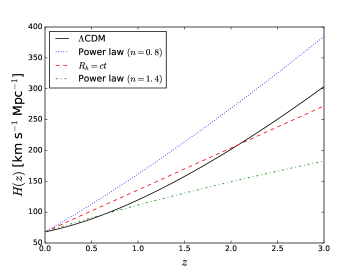
Figure 1: Hubble parameter as a function of the redshift for $\Lambda$CDM, $R_{h}=ct$ cosmology and two different power law cosmologies. $\Omega_{m}$, $\Omega_{r}$ and $H_{0}$ have been fixed to $0.3$, $8\times 10^{-5}$ and $68\,\text{km}\,\text{s}^{-1}\text{Mpc}^{-1}$, respectively, for illustrative purposes.

III METHOD

In this section we review the statistical tools used to quantify the goodness of fit and to compare the models under study.

III.1 Goodness of fit

To quantify the capacity of a model to fit the data we minimize the common $\chi^{2}$ function,

$$\chi^{2}=(\textbf{u}-\textbf{u}_{data})^{T}C^{-1}(\textbf{u}-\textbf{u}_{data})\,,$$ (10)

using the MIGRAD application from the iminuit Python package, designed for finding the minimum value of a multiparameter function and analyzing the shape of the function around the minimum. This code is the Python implementation of the former MINUIT Fortran code minuit . In Eq. (10), u stands for the model prediction, while $\textbf{u}_{data}$ and $C^{-1}$ hold for the observables and their inverse covariance matrix, respectively. We then compute the probability that a larger value for the $\chi^{2}$ could occur for a fit with $\nu=N-k$ degrees of freedom, where $N$ is the number of data points and $k$ is the number of free parameters of the model,

$$P(\chi^{2},\nu)=\frac{\Gamma\left(\frac{\nu}{2},\frac{\chi^{2}}{2}\right)}{\Gamma\left(\frac{\nu}{2}\right)}\,,$$ (11)

with $\Gamma(t,x)$ being the upper incomplete gamma function and $\Gamma(t)=\Gamma(t,0)$ the complete gamma function.

Obtaining a probability close to 1 implies that it is very likely to get larger $\chi^{2}$ values, meaning that the model fits correctly (possibly too well) the data. On the other hand, obtaining a small probability indicates that the model does not provide a good fit to the data.

When combining probes, we minimize the $\chi^{2}$ function given by the sum of individual $\chi^{2}$ functions, i.e., we assume that the probes are statistically independent.

It is important to notice that Eq. (11) is only valid when we work with $N$ data points coming from $N$ independent random variables with Gaussian distributions. However, in this work we consider the correlation within probes; thus, the data points come from nonindependent Gaussian random variables. In order to check the impact of correlations on this probability we compute the histogram of $\chi^{2}$ through Monte Carlo simulations with and without correlations. First of all, we fix the fiducial model to $\textbf{u}=\textbf{0}$ in order to save computation time, since we do not need then to fit a certain model each time we compute a $\chi^{2}$. Notice that there are no parameters then; thus, $k=0$ and $\nu=N$. We then generate the data set from an $N$-dimensional Gaussian distribution centered at 0 and with the corresponding covariance matrix $C$ for the probes used. When neglecting correlations we consider only the diagonal terms of $C$. Finally, we compute the $\chi^{2}$ using Eq. (10) and we repeat $M$ times to obtain the histograms shown in Fig. 2.

In the left plot we use the covariance matrix for BAO and CMB data. We can clearly observe that the histogram obtained with correlations (green) is completely consistent with the histogram obtained neglecting any correlation (purple). Moreover, both of them are consistent with the analytic distribution (thick black solid line), which is given by the derivative of Eq. (11) with respect to $\chi^{2}$. Notice that we have neglected here the number of free parameters of the model because we have fixed the fiducial model to 0. The fact that the three distributions are completely consistent implies that the correlations in the BAO+CMB covariance matrix do not effect Eq. (11) and we can safely use it. In the right plot of Fig. 2 we have the equivalent results using the covariance matrix for SNIa, BAO and CMB. As before, the three distributions are completely consistent, implying that we can use Eq. (11) with these correlations. A particularity in this case is that the covariance matrix is not completely independent of the cosmology. As is discussed in the following sections, the covariance matrix depends on two nuisance parameters. In order to correctly predict the effect of these correlations, we need to consider these nuisance parameters and determine them when fitting each model under study to the $M$ mock data samples. However, we keep the fiducial $\textbf{u}=\textbf{0}$ model, due to the fact that the two SNIa nuisance parameters remain very close to $\alpha=0.14$ and $\beta=3.1$, as can be seen in Table 1.

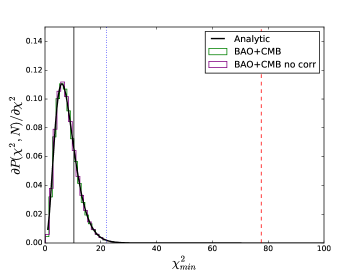
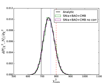
Figure 2: Histograms of $\chi^{2}$ for Monte Carlo simulations [to study the impact of correlations in Eq. (11)] using correlations (green) and neglecting them (purple). The analytic distribution is also represented for further comparison (thick black solid line). The compatibility of the three distributions in each plot shows that Eq. (11) can be used in this work. The measured values of the minimum of the $\chi^{2}$ are also represented, only for illustrative purposes, for each model and each combination of probes used (see Table 2. Black solid line, $\Lambda$CDM; blue dotted line, power law cosmology; red dashed line, $R_{h}=ct$ cosmology). Left plot: BAO+CMB covariance matrix with $M$=100000 iterations. Right plot: SNIa+BAO+CMB covariance matrix with $M$=10000 iterations.

III.2 Model comparison

In this work we consider two widely used criteria to compare the models under study: the Akaike information criterion (AIC) AIC and the Bayesian information criterion (BIC) BIC . Both account for the fact that a model with fewer parameters is generally preferable to a more complex model if both of them fit the data equally well.

The AIC is built from information theory. Rather than having a simple measure of the direct distance between two models (Kullback-Leibler distance), the AIC provides us with an estimate of the expected, relative distance between the fitted model and the unknown true mechanism that actually generated the observed data. We must be aware that the AIC is useful in selecting the best model in the set of tested models; however, if all the models are very poor, the AIC still gives us the one estimated to be the best. This is why we previously computed the probability of a model to correctly fit the data [see Eq. (11)]. Given the minimum of the $\chi^{2}$ ($\chi^{2}_{min}$) and the number of free parameters of the model $k$, the AIC is given by

$$\text{AIC}=\chi^{2}_{min}+2k\,.$$ (12)

The AIC may perform poorly if there are too many parameters compared to the size of the sample AICc1 ; AICc2 . In this case, a second-order variant of the AIC can be used, the so-called AICc AICc25 ,

$$\text{AICc}=\text{AIC}+\frac{2k(k+1)}{N-k-1}\,,$$ (13)

where $N$ is the number of data points. An extensive presentation and discussion of the AIC and its variations can be found in AICc3 .

The BIC is one of the most used criterion from the so-called dimension-consistent criteria (see BIC1 for a review of many of these criteria). It was derived in a Bayesian context with equal prior probability on each model and minimal priors on the parameters, given the model. It is given by

$$\text{BIC}=\chi^{2}_{min}+k\ln(N)\,.$$ (14)

Both the AICc and the BIC strongly depend on the size of the sample. In order to compare different models we use the exponential of the differences $\Delta$AICc/2 ($\Delta$BIC/2), where $\Delta$AICc=$\text{AICc}_{\Lambda\text{CDM}}$-AICc (Id. for the BIC), since the exponential can be interpreted as the relative probability that the corresponding model minimizes the estimated information loss with respect to the $\Lambda$CDM model.

Given that the AIC (AICc) and the BIC can both be derived as either frequentist or Bayesian procedures, what fundamentally distinguishes them is their different philosophy, including the nature of their target models. Thus, the choice of the criterion depends on their performance under realistic conditions. A comparison of these two criteria is outside the scope of this paper (see COMP for an extended and detailed comparison), so we just provide the results for both of them. In general, though, the BIC penalizes extra parameters more severely than the AIC.

It is important to notice that when comparing two models with the same data sample and the same number of parameters (e.g. $\Lambda$CDM and power law with SNIa data, $N=740$, $k=5$), $\Delta$AIC and $\Delta$BIC basically reduce to $\Delta\chi^{2}_{min}=\chi^{2}_{\Lambda\text{CDM}}-\chi^{2}$. This leads to the same numerical values for exp$(\Delta\text{AICc}/2)$ and exp$(\Delta\text{BIC}/2)$ for $\Lambda$CDM and power law models in Table 2.

IV Low-redshift probes

In this section we describe the two low-redshift cosmological probes and the corresponding data sets used to compare the different models presented.

IV.1 SNIa

Type Ia supernovae are considered as standardizable candles useful to measure cosmological distances. Although measurements of CMB and large-scale structure can constrain the matter content of the Universe and the dark energy equation of state parameter, SNIa are important for breaking degeneracies and achieve precise cosmological measurements. The observable used in SNIa measurements is the so-called distance modulus,

$$\mu(z)=5\log_{10}\left(\frac{H_{0}}{c}d_{L}(z)\right)\,,$$ (15)

where $d_{L}(z)=(1+z)r(z)$ is the luminosity distance. Notice that we have defined the distance modulus in such a way that it is independent of the $H_{0}$ parameter, which is degenerate with the SNIa absolute magnitude.

Distance estimation with SNIa is based on empirical observation that these events form a homogeneous class whose variability can be characterized by two parameters Tripp1998 : the time stretching of the light curve ($X_{1}$) and the supernova color at maximum brightness ($C$). In this work we use the joint light-curve analysis for SNIa from Betoule2014 . The authors assume that supernovae with identical color, shape and galactic environment have on average the same intrinsic luminosity for all redshifts. This yields the distance modulus,

$$\mu_{\text{obs}}=m_{B}^{*}-(M_{B}-\alpha\times X_{1}+\beta\times C)\,,$$ (16)

where $m_{B}^{*}$ corresponds to the observed peak magnitude in the rest-frame B band and $\alpha$ and $\beta$ are nuisance parameters in the distance estimate. The $M_{B}$ nuisance parameter is given by the step function,

$$M_{B}=\left\{\begin{array}[]{cl}M_{B}^{1}\,,&\text{if }M_{\text{stellar}}<10^{10}M_{\odot}\,,\\ M_{B}^{1}+\Delta M\,,&\text{otherwise}\,,\end{array}\right.$$ (17)

where $M_{B}^{1}$ and $\Delta M$ are nuisance parameters, in order to take into account the dependence on host galaxy properties.

Concerning the errors and correlations on the measurements we use the covariance matrix provided by Betoule2014 where the authors consider the contribution from error propagation of light-curve fit uncertainties (statistical contribution) and the contribution of seven sources of systematic uncertainty: the calibration, the light-curve model, the bias correction, the mass step, the dust extinction, the peculiar velocities and the contamination of nontype Ia supernovae.

In some specific cases during this work we relax the redshift independence assumption made in Betoule2014 . In order to account for a possible SNIa evolution with redshift (caused by some astrophysical procedures, for example, see SNIaevI ; SNIaevII for previous studies accounting for SNIa evolution) we add an extra nuisance parameter $\epsilon$ to the distance modulus estimate,

$$\mu_{\text{obs}}=m_{B}^{*}-(M_{B}-\alpha\times X_{1}+\beta\times C-\epsilon\times z)\,.$$ (18)

When using SNIa data, the set of nuisance parameters considered is $\{\alpha,\,\beta,\,M,\,\Delta M,\,\epsilon\}$. For $\Lambda$CDM and the power law cosmology we consider $\Omega_{m}$ and $n$, respectively, as cosmological parameters. We consider no cosmological parameters when using SNIa data with the $R_{h}=ct$ cosmology.

IV.2 BAO

The baryonic acoustic oscillations are the regular and periodic fluctuations of visible matter density in large-scale structure. They are characterized by the length of a standard ruler, generally denoted by $r_{d}$. The main observable used in BAO measurements is the ratio of the BAO distance at low redshift to this scale $r_{d}$. In the $\Lambda$CDM model, the BAO come from the sound waves propagating in the early Universe and the standard ruler $r_{d}$ is equal to the comoving sound horizon at the redshift of the baryon drag epoch: $r_{d}=r_{s}(z_{d})$, $z_{d}\approx 1060$. For models differing from the $\Lambda$CDM model, $r_{d}$ does not need to coincide with $r_{s}(z_{d})$ Verde . For the moment, and in order to be as general as possible, we do not delve into the physics governing the sound horizon $r_{d}$, so we consider $r_{d}$ as a free parameter.

The BAO are usually assumed to be isotropic. In this case the BAO distance scale is given by

$$D_{V}(z)\equiv\left(r^{2}(z)\frac{cz}{H(z)}\right)^{1/3}\,.$$ (19)

More recently it has also been possible to measure radial and transverse clustering separately, allowing for anisotropic BAO. The BAO distance scales are then $r(z)$ and $c/H(z)$.

In this work we follow Aubourg in combining the measurements of 6dFGS BAO1 , SDSS [Main Galaxy Sample (MGS)] BAO2 , BOSS (CMASS and LOWZ samples - Data Release 11) BAO3 ; Anderson2014 and BOSS Lyman-$\alpha$ forest (Data Release 11) BAO5 ; BAO6 . As in Shafer , we assume that all the measurements are independent, apart from the CMASS anisotropic measurements (correlated with coefficient -0.52) and the Lyman-$\alpha$ forest measurements (correlated with coefficient -0.48).

According to Bassett , when constraining parameters to a high confidence level or claiming that a model is a poor fit to the data, one should take into account that BAO observable likelihoods are not Gaussian far from the peak. In this work we follow the same approach and account for this effect by replacing the usual $\Delta\chi^{2}_{G}=-2\ln\mathcal{L}_{G}$ for a Gaussian likelihood observable by

$$\Delta\chi^{2}=\frac{\Delta\chi^{2}_{G}}{\sqrt{1+\Delta\chi^{4}_{G}\left(\frac{S}{N}\right)^{-4}}}\,,$$ (20)

where $S/N$ is the corresponding detection significance, in units of $\sigma$, of the BAO feature. We consider a detection significance of 2.4$\sigma$ for 6dFGS, 2$\sigma$ for SDSS MGS, 4$\sigma$ for BOSS LOWZ, 6$\sigma$ for BOSS CMASS and 4$\sigma$ for BOSS Lyman-$\alpha$ forest.

When using BAO data, we consider the following set of cosmological parameters: $\{r_{d}\times H_{0}/c,\,\Omega_{m},\,n\}$. The latter two only apply for $\Lambda$CDM and power law cosmology, respectively. We do not consider any nuisance parameter.

V High-redshift probe: CMB

In this section we present the high-redshift probe used, the cosmic microwave background, and the approach we follow in order to consider this probe in our study, including power law models.

The CMB is an extremely powerful source of information due to the high precision of modern data. Furthermore it represents high redshift data, complementing low-redshift probes. In standard cosmology, the physics governing the sound horizon at the early Universe is that of a baryon-photon plasma in an expanding Universe. The comoving sound horizon at the last scattering redshift is given by

$$r_{s}(z_{*})=\int_{z_{*}}^{\infty}\frac{c_{s}(z)\,\text{d}z}{H(z)}\,,$$ (21)

where $z_{*}$ stands for the redshift of the last scattering and where

$$c_{s}(z)=\frac{c}{\sqrt{3(1+R_{b}(z))}},\hskip 15.0ptR_{b}(z)=\frac{3\rho_{b}}{4\rho_{\gamma}}\,,$$ (22)

with $\rho_{b}$ being the baryon density and $\rho_{\gamma}$ the photon density. The observed angular scale of the sound horizon at recombination,

$$\ell_{a}\equiv\frac{\pi c}{r_{s}(z_{*})}\int_{0}^{z_{*}}\frac{\text{d}z}{H(z)}\,,$$ (23)

then depends on the angular distance to the CMB, a physical quantity sensitive to the expansion history up to $z_{*}$ and thereby to the background history of models CMB1 . Notice that $\ell_{a}$ roughly corresponds to the position of the first peak of the temperature angular power spectrum of the CMB. Although this represents a reduced fraction of the information, it is well known that reduced parameters capture a large fraction of the information contained in the CMB fluctuations of the angular power spectra Wang . We use the value provided by the Planck Collaboration Planck2015noMG : $\ell_{a}=301.63\pm 0.15$ and, in the following, we refer to this information as CMB data. It has been obtained from Planck temperature and low-$\ell$ polarization data. Marginalization over the amplitude of the lensing power spectrum has been performed, since it leads to a more conservative approach.

According to Melia2015 , the $R_{h}=ct$ universe assumes the presence of dark energy and radiation in addition to baryonic and dark matter. The only requirement of this model is to constrain the total equation of state by requiring $\rho+3p=0$. Following this definition, and extending the idea to the power law cosmology, we infer that the physics governing the sound horizon at the early Universe is the same as for $\Lambda$CDM, since we are again essentially dealing with a baryon-photon plasma in an expanding universe.

For $\Lambda$CDM, we use the value provided in Planck2015table for $\Omega_{b}h^{2}=0.02230$ and we use Eq. (4) for the radiation contribution. This assumption has already been made in the literature. In Levy , for example, the authors considered the Dirac-Milne universe (a matter-antimatter symmetric cosmology) and kept the same expression for $r_{s}(z_{*})$ as in the $\Lambda$CDM case.

For a power law cosmology,

$$r_{s}(z_{*})\propto\int_{z_{*}}^{\infty}\frac{(1+z)^{1/2}}{(1+z)^{1/n}}\,\text{d}z\,$$ (24)

which converges only for $n<2/3$; therefore, there is already a fundamental problem in these theories when describing the early Universe. This divergence also exists for the sound horizon $r_{d}$ in the BAO. Given that the big bang nucleosynthesis already suffers from a problem in the early Universe, one might imagine that the physics of the early Universe allows us to solve this issue, essentially by restoring the standard model in the very early Universe, keeping the sound horizon finite. $r_{d}$ being now an unknown quantity, we have to obtain its value by fitting it to the data. We can then develop $r_{s}(z_{*})$ by,

$$r_{s}(z_{*})=\int_{z_{*}}^{\infty}\frac{c_{s}(z)\,\text{d}z}{H(z)}=r_{d}-\int_{z_{d}}^{z_{*}}\frac{c_{s}(z)\,\text{d}z}{H(z)}\,.$$ (25)

In Levy the authors also had to deal with this divergence near the initial singularity. They opted for putting upper and lower bounds to the integral on physically motivated grounds, while we allow the data to determine $r_{d}$ and avoid the divergence.

We now need to determine $z_{d}$ and $z_{*}$ for all the models. A common definition of the redshift of the CMB is given by the maximum of the visibility function Hu96 ,

$$g(z)=\dot{\tau}(z)e^{-\tau(z)}\,,$$ (26)

where $\tau(z)$ is the optical depth tau ,

$$\tau(z)=\sigma_{T}\int_{0}^{z}n_{e}(z^{\prime})\frac{c}{(1+z^{\prime})H(z^{\prime})}\,\text{d}z^{\prime}\,,$$ (27)

with $\sigma_{T}$ being the Thomson cross section and $n_{e}$ the free electron number density. This definition is well motivated because the visibility function can be understood as the probability of the last photons of the CMB to scatter; thus, the maximum provides us with the most probable redshift of this last scattering. In order to obtain $n_{e}$ we calculate the free electron fraction $X_{e}$ and we further multiply it by the hydrogen number density,

$$n_{e}(z)=X_{e}(z)\left[\frac{3H_{0}^{2}\Omega_{b}}{8\pi Gm_{H}\mu}(1+z)^{3}\right]\,,$$ (28)

where $m_{H}$ is the mass of the hydrogen atom and $\mu=1/(1-Y)$ with $Y$ being the helium mass fraction.

The ionization history $X_{e}(z)$ depends on the expansion rate. In order to obtain it we use the Recfast++ Recfast++ code, based on the C version of Recfast Recfast , adapting the expansion history to the corresponding one for each model. This new version includes recombination corrections Recfast++ ; RubinoMartin and allows us to run a dark matter annihilation module Chluba . It also includes a new ordinary differential equations solver ODE . More details about this code can be found in Recfast++1 ; Recfast++2 ; Recfast++3 . Figure 3 provides a comparison between $X_{e}$ for the different power law cosmologies and $\Lambda$CDM. We have neglected the recombination corrections and dark matter annihilations for simplicity, and because this level of precision in the $X_{e}$ determination is not needed for our purposes.

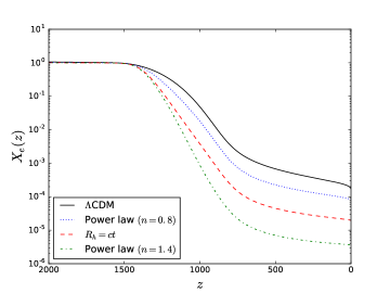
Figure 3: Free electron function $X_{e}$ as a function of the redshift for $\Lambda$CDM, $R_{h}=ct$ cosmology and two different power law cosmologies. The parameters relevant for reionization have been fixed to the Planck 2015 values for illustrative purposes Planck2015table (helium mass fraction, CMB temperature at $z=0$, $\Omega_{m}$, $\Omega_{b}$, $\Omega_{k}$, $h$ and $N_{\text{eff}}$).

Another definition for the redshift of the CMB is the one adopted by the Planck Collaboration Planck2015table by determining the redshift when the optical depth equals 1. We denote $z_{CMB}$ the redshift obtained with the first definition [Eq. (26)] and $z_{*}$ the redshift obtained with the Planck Collaboration convention. Although we use $z_{*}$ for consistency with Planck when performing our analyses, we have defined $z_{CMB}$ for illustrative and comparative purposes.

In Fig. 4 we show the visibility functions for $\Lambda$CDM, $R_{h}=ct$ cosmology and two power law cosmologies ($n=0.8$ and $n=1.4$). In this case we have fixed the cosmological parameters to $\Lambda$CDM present-day values: $Y=0.249,\,\Omega_{m}=0.3089,\,\Omega_{b}=0.0485976,\,N_{\text{eff}}=3.04$ and $H_{0}=67.74\,\text{km}\,\text{s}^{-1}\text{Mpc}^{-1}$ Planck2015table . However, we have checked that any variation of 25% in one of these parameters has a negligible impact on the redshift of the CMB (less than 0.6%) for a fixed model and that it has no influence in our study. Even if the redshift of the CMB does not change significantly with the parameters, it does change with the model; therefore we fix $z_{*}=1090.71$ for $\Lambda$CDM and $z_{*}=1055.05$ for the $R_{h}=ct$ cosmology. Concerning the power law cosmology, since the redshift changes significantly with $n$, we interpolate $z_{*}$ as a function of $n$.

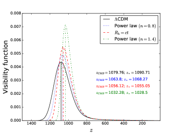
Figure 4: Visibility function as a function of the redshift for $\Lambda$CDM (black), $R_{h}=ct$ cosmology (red) and $n=0.8,\,1.4$ power law cosmologies (blue and green, respectively). We show the redshift of the CMB computed with two different definitions (see the text for details).

The redshift of the baryon drag epoch can be defined in two analogous ways. We first consider the definition given by a drag visibility function Hu96 ,

$$g_{d}(z)=\dot{\tau}_{d}(z)e^{-\tau_{d}(z)}\,,$$ (29)

where the drag optical depth is given by,

$$\tau_{d}(z)=\int_{0}^{z}\frac{\dot{\tau}(z^{\prime})}{R_{b}(z^{\prime})}\,\text{d}z^{\prime}\,.$$ (30)

We denote the maximum of this drag visibility function $z_{drag}$. The second definition (the one adopted by the Planck Collaboration Planck2015table ) is given by the redshift at which the drag optical depth equals 1. We denote it $z_{d}$. As before, we use $z_{d}$ to be consistent with Planck, but we keep both definitions for illustrative and comparative purposes.

In Fig. 5 we show the drag visibility functions for the same models that appear in Fig. 4. The cosmological parameters are fixed to the same present-day values Planck2015table and we have also checked that any variation of 25% in one of the parameters does not lead to significant changes in our results. Therefore, we fix $z_{d}=1060.61$ for $\Lambda$CDM and $z_{d}=1031.85$ for the $R_{h}=ct$ cosmology. As for $z_{*}$ we observe that $z_{d}$ changes significantly with the exponent of the power law cosmology; thus, we interpolate $z_{d}$ as a function of $n$.

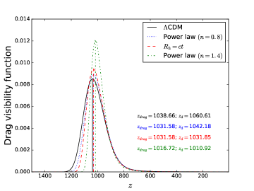
Figure 5: Drag visibility function as a function of the redshift for $\Lambda$CDM (black), $R_{h}=ct$ cosmology (red) and $n=0.8,\,1.4$ power law cosmologies (blue and green, respectively). The redshift of the drag epoch computed with two different definitions is presented (see the text for details).

No extra cosmological or nuisance parameters are considered when including the CMB data.

VI RESULTS

In Table 1 we present the best-fit values obtained for the different cosmological and nuisance parameters of the models studied with the different probes used. In Table 2 we show the results of the goodness of fit and model comparisons. More specifically, we report the number of parameters of the model, the number of data points used, the minimum value for the $\chi^{2}$ function, the goodness of fit statistic and the exponential of the differences $\Delta$AICc$/2$ and $\Delta$BIC$/2$.

Focusing first on the SNIa alone, Fig. 6 provides the residuals to the best-fit (normalized to the $\Lambda$CDM model) for each model. $\Lambda$CDM provides a very good fit to the data $(P(\chi^{2},\nu)=0.915$), as well as the power law cosmology $(P(\chi^{2},\nu)=0.915$, with $n=1.55\pm 0.13)$. Although the $R_{h}=ct$ cosmology provides a slightly worse fit $(P(\chi^{2},\nu)=0.644)$, it is still acceptable. However, it is highly disfavored when considering the model comparison statistics $(\text{exp}(\Delta\text{AICc}/2)=1.308\times 10^{-8}$ and exp$(\Delta\text{BIC}/2)=1.291\times 10^{-7})$. Despite the fact that the $R_{h}=ct$ model has fewer parameters than $\Lambda$CDM, the $\chi^{2}$ difference is large enough $(\Delta\chi^{2}=38.33)$ to compensate for the preference of the $R_{h}=ct$ model coming from the Occam factor of the AIC and the BIC. By Occam factor we mean here the non-$\chi^{2}$ term in Eqs. (13) and (14).

Figure 6: Fit from the three models under study to the SNIa data. All the plots show the residuals with respect to the prediction from $\Lambda$CDM with the best-fit values. Top panel: SNIa measurements standardized to $\Lambda$CDM (black) and $\Lambda$CDM prediction (red) as a function of the redshift. Central panel: SNIa measurements standardized to power law cosmology (green) and power law cosmology prediction (blue) as a function of the redshift. Bottom panel: SNIa measurements standardized to $R_{h}=ct$ cosmology (purple) and $R_{h}=ct$ cosmology prediction (orange) as a function of the redshift. For each model we marginalize over the nuisance parameters.

In Fig. 7 we present the residuals of the fit to the BAO data alone from the three models under study. From the top panel we immediately see that $\Lambda$CDM is not a good fit to BAO data $(P(\chi^{2},\nu)=0.088)$. This tension has already been noted in the literature Aubourg ; Shafer and is due to the anisotropic Lyman-$\alpha$ forest BAO measurements at high redshift $(z=2.34)$. Since SNIa and BAO prefer similar values of $\Omega_{m}$, no extra tension appears when combining these probes. The power law cosmology provides a better fit to BAO data than $\Lambda$CDM $(P(\chi^{2},\nu)=0.531)$ implying preference of the power law cosmology over $\Lambda$CDM from the model comparison statistics $(\text{exp}(\Delta\text{AICc}/2)=$exp$(\Delta\text{BIC}/2)=15.198)$. Regarding the $R_{h}=ct$ model, the fit is worse than for $\Lambda$CDM $(P(\chi^{2},\nu)=0.016)$, but the difference of $\chi^{2}$ with respect to $\Lambda$CDM is nearly compensated by the Occam factor, so that the model has commensurate values of the AICc and the BIC: $\text{exp}(\Delta\text{AICc}/2)=0.385$ and exp$(\Delta\text{BIC}/2)=0.125$, respectively.

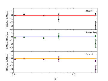
Figure 7: Fit from the three models under study to the BAO data. Each plot shows the residuals with respect to the corresponding model. The isotropic measurements of the BAO are represented with a circle and their observable is $D_{V}(z)/r_{d}$, while the stars stand for the radial measurements with observable $r(z)/r_{d}$ and the squares stand for the transverse measurements with observable $c/(H(z)r_{d})$. Top panel: BAO measurements (black) and $\Lambda$CDM prediction (red) as a function of the redshift. Central panel: BAO measurements (green) and power law cosmology prediction (blue) as a function of the redshift. Bottom panel: BAO measurements (purple) and $R_{h}=ct$ cosmology prediction (orange) as a function of the redshift.

In Fig. 8 we show the results from fitting the three models to SNIa and BAO data simultaneously. In the left panel we present the fits from the models to SNIa data using the best-fit values obtained from both SNIa and BAO data. These results are very similar to the ones obtained for SNIa alone (Fig. 6), showing that adding the BAO does not affect the SNIa-related parameters. In the right panel of Fig. 8 we show the fit from the models to BAO data, using the SNIa+BAO best-fit values for the parameters. We notice that the power law cosmology provides a slightly worse fit than when considering BAO data alone (Fig. 7). Looking at the goodness of fit for SNIa and BAO data, we find that the power law cosmology provides a slightly worse fit $(P(\chi^{2},\nu)=0.833$) than the $\Lambda$CDM $(P(\chi^{2},\nu)=0.898)$, which is also the case for the $R_{h}=ct$ cosmology $(P(\chi^{2},\nu)=0.546)$. Despite the small difference between the power law cosmology and the $\Lambda$CDM fits, the model comparison statistics tell us that the latter is preferred $(\text{exp}(\Delta\text{AICc}/2)=$exp$(\Delta\text{BIC}/2)=0.0036)$. The $R_{h}=ct$ cosmology is even more strongly disfavored with respect to $\Lambda$CDM than when considering SNIa data alone $(\text{exp}(\Delta\text{AICc}/2)=6.251\times 10^{-10}$ and exp$(\Delta\text{BIC}/2)=6.184\times 10^{-9})$.

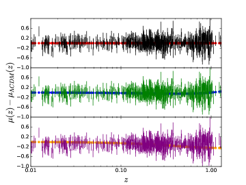
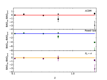
Figure 8: Fit from the three models under study to the SNIa and BAO data; i.e. the parameter values of the models are the best-fit values from SNIa+BAO data. Left plot: SNIa residuals with respect to the prediction from $\Lambda$CDM with the best-fit values, for the three models under study (see Fig. 6). Right plot: BAO residuals with respect to the model under study (see Fig. 7).

From these results (the best-fit values are nearly all consistent with Shafer within 1$\sigma$) we deduce that $R_{h}=ct$ is very disfavored with respect to $\Lambda$CDM, while the power law cosmology is slightly disfavored with respect to $\Lambda$CDM.

In order to be more conservative we allow for some SNIa evolution with the redshift [Eq. (18)]. In Fig. 9 we have the results for SNIa data. We can observe that now all the models provide a very good fit to the data. Interestingly, the evolution nuisance parameter is nearly consistent with 0 for $\Lambda$CDM and the power law cosmology, while it is clearly non-null for the $R_{h}=ct$ cosmology. This is completely consistent since the $\Lambda$CDM and the power law cosmology were already able to provide a good fit without evolution, while the $R_{h}=ct$ needed this nuisance term in order to correctly fit the data. From the model comparison statistics we can deduce that there is no clear preference for one model over another.

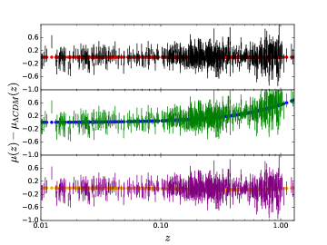
Figure 9: Fit from the three models under study to the SNIa data allowing for some evolution with the redshift. All the plots show the residuals with respect to the prediction from $\Lambda$CDM with the best-fit values (see Fig. 6). The introduction of some evolution with the redshift modifies the observed $\mu(z)$ giving a good fit for all the models.

Now we can combine the SNIa data (allowing for evolution) with the BAO data. The results are shown in Fig. 10. Contrary to what we have seen in Fig. 8, adding the BAO does modify the SNIa-related parameter values, but we still obtain a very good fit to the SNIa data using the best-fit values obtained from SNIa+BAO data and allowing for evolution. Concerning the fit to BAO data, using this combination of data to determine the best-fit values, we recover the results obtained with BAO data alone (Fig. 7). This shows that when we relax the redshift independence for SNIa, the power in model selection from the combination of SNIa and BAO weakens. As the power law cosmology was slightly preferred over $\Lambda$CDM when considering BAO data alone, it is not surprising that it is also the case here $(\text{exp}(\Delta\text{AICc}/2)=$exp$(\Delta\text{BIC}/2)=3.421)$. Concerning the $R_{h}=ct$ cosmology, the Occam factor is nearly as important as the $\chi^{2}$ difference and it leads to only a marginal preference for the $\Lambda$CDM $(\text{exp}(\Delta\text{AICc}/2)=0.046$ and exp$(\Delta\text{BIC}/2)=0.455)$.

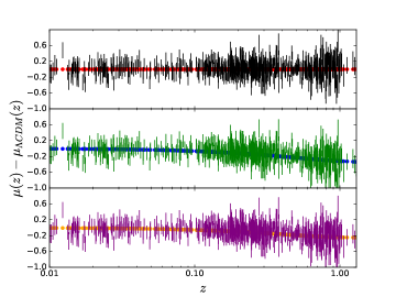
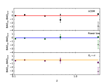
Figure 10: Fit from the three models under study to the SNIa and BAO data allowing for redshift evolution for the SNIa; i.e. the parameter values of the models are the best-fit values from SNIa+evolution+BAO data. Left plot: SNIa residuals with respect to the prediction from $\Lambda$CDM with the best-fit values (see Fig. 6). Right plot: BAO residuals with respect to the model under study (see Fig. 7). Allowing for some redshift evolution for SNIa provides a good fit for the three models to both SNIa and BAO data.

From these results we can deduce that adding a redshift evolution in the SNIa as a nuisance parameter leads to no clear preference of one model over another.

We finally consider the addition of CMB data. Notice that in this work we cannot combine CMB and SNIa data, since we rely on the BAO scale to introduce the CMB scale (see Sec. V); therefore we always need to consider BAO data when including the CMB. The results for BAO and CMB data are shown in Fig. 11 and in Table 3. In the plot we have the results for BAO data with the best-fit values obtained with BAO and CMB data. In the table we present the value of $\ell_{a}$ for each model with the BAO and CMB data best-fit values. We can see that there is no evolution in the $\Lambda$CDM BAO fit when we add the CMB information to determine the best-fit values, as expected. However, adding the CMB information is crucial for the power law and the $R_{h}=ct$ cosmologies, since the fit to the BAO data is strongly degraded [$P(\chi^{2},\nu)=1.2\times 10^{-3}$ and $P(\chi^{2},\nu)=4.4\times 10^{-14}$, respectively]. From the model comparison point of view, the power law cosmology is disfavored $(\text{exp}(\Delta\text{AICc}/2)=$exp$(\Delta\text{BIC}/2)=0.0029)$ and the $R_{h}=ct$ cosmology is strongly disfavored $(\text{exp}(\Delta\text{AICc}/2)=1.680\times 10^{-14}$ and exp$(\Delta\text{BIC}/2)=7.349\times 10^{-15})$ with respect to $\Lambda$CDM.

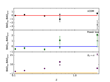
Figure 11: Fit from the three models under study to the BAO and CMB data. All the plots show the BAO residuals with respect to the model under study (see Fig. 7). The introduction of the CMB data strongly degrades (notice the increase in the Y-axis limits and the small size of the error bars) the fit to BAO data for the power law and the $R_{h}=ct$ cosmologies.

We can now combine the information from the three probes: SNIa, BAO and CMB. The results are presented in Fig. 12 and in Table 3. From the left plot we can see that adding the CMB information does not affect the fit to SNIa (see the left panel of Fig. 10). However, it completely degrades the fit to the BAO data for the power law and the $R_{h}=ct$ cosmologies (see the right panel of Figs. 10 and 11). In terms of model comparison the power law cosmology is very disfavored $(\text{exp}(\Delta\text{AICc}/2)=$exp$(\Delta\text{BIC}/2)=2.501\times 10^{-15})$ and the $R_{h}=ct$ cosmology is extremely disfavored $(\text{exp}(\Delta\text{AICc}/2)=3.598\times 10^{-23}$ and exp$(\Delta\text{BIC}/2)=3.562\times 10^{-22})$ with respect to $\Lambda$CDM. It is important to notice here that the $\chi^{2}$ and the $P(\chi^{2},\nu)$ obtained for the $R_{h}=ct$ and the power law cosmologies are acceptable, but the model criteria tell us that these models are highly improbable. This is due to the introduction of SNIa data. Both models provide an acceptable fit to these data; so, when including so many data points, the global fit is still acceptable. However, the model criteria are essentially sensitive to the exponential of the difference of $\chi^{2}$, so they can distinguish between different models approximately fitting the data. It is a clear example between the difference of correctly fitting the data and being better than another model.

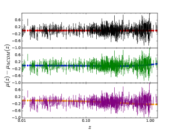
Figure 12: Fit from the three models under study to the SNIa, BAO and CMB data; i.e. the parameter values of the models are the best-fit values from SNIa+BAO+CMB data. Left plot: SNIa residuals with respect to the prediction from $\Lambda$CDM with the best-fit values (see Fig. 6). Right plot: BAO residuals with respect to the model under study (see Fig. 7).

For completeness and in order to be as conservative as possible, we also consider a redshift evolution of SNIa. The results are shown in Fig. 13 and in Table 3. From the left plot we notice that adding the evolution leads to very good fits to SNIa data. However, from the right plot we can see that the redshift evolution in SNIa is not sufficient to compensate for the effect of the CMB; thus the power law and $R_{h}=ct$ cosmologies are not able to correctly fit the BAO data. The results from the model comparison still remain clear, showing that $\Lambda$CDM is very strongly preferred over the power law $(\text{exp}(\Delta\text{AICc}/2)=$exp$(\Delta\text{BIC}/2)=3.127\times 10^{-15})$ and the $R_{h}=ct$ $(\text{exp}(\Delta\text{AICc}/2)=2.363\times 10^{-15}$ and exp$(\Delta\text{BIC}/2)=2.332\times 10^{-14})$ cosmologies.

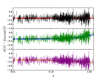
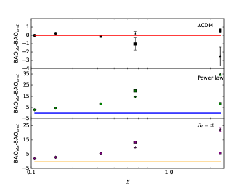
Figure 13: Fit from the three models under study to the SNIa, BAO and CMB data and allowing for redshift evolution for the SNIa; i.e. the parameter values of the models are the best-fit values from SNIa+evolution+BAO+CMB data. Left plot: SNIa residuals with respect to the prediction from $\Lambda$CDM with the best-fit values (see Fig. 6). Right plot: BAO residuals with respect to the model under study (see Fig. 7). Allowing for some redshift evolution for the SNIa is not sufficient to compensate for the effect of the CMB, and we remain with a poor fit for the power law and $R_{h}=ct$ cosmologies.

Table 1: Best-fit values for the cosmological and nuisance parameters of the studied models with different cosmological probes.

		$\Omega_{m}$	$n$	$r_{d}\times H_{0}/c$	$\alpha$	$\beta$	$M$	$\Delta M$	$\epsilon$
$\Lambda$CDM	SNIa	$0.295\pm 0.034$	-	-	$0.1412\pm 0.0066$	$3.101\pm 0.081$	$24.110\pm 0.023$	$-0.070\pm 0.023$	-
	BAO	$0.289\pm 0.021$	-	$0.03377\pm 0.00057$	-	-	-	-	-
	SNIa+BAO	$0.291\pm 0.018$	-	$0.03373\pm 0.00050$	$0.1413\pm 0.0066$	$3.103\pm 0.080$	$24.110\pm 0.019$	$-0.070\pm 0.023$	-
	SNIa+ev	$0.49\pm 0.17$	-	-	$0.1410\pm 0.0066$	$3.100\pm 0.081$	$24.120\pm 0.025$	$-0.070\pm 0.023$	$-0.23\pm 0.19$
	SNIa+ev+BAO	$0.291\pm 0.021$	-	$0.03373\pm 0.00057$	$0.1413\pm 0.0066$	$3.103\pm 0.081$	$24.110\pm 0.022$	$-0.070\pm 0.023$	$-0.001\pm 0.055$
	BAO+CMB	$0.307\pm 0.011$	-	$0.03348\pm 0.00049$	-	-	-	-	-
	SNIa+BAO+CMB	$0.306\pm 0.010$	-	$0.03353\pm 0.00045$	$0.1411\pm 0.0066$	$3.098\pm 0.080$	$24.110\pm 0.018$	$-0.070\pm 0.023$	-
	SNIa+ev+BAO+CMB	$0.308\pm 0.011$	-	$0.03345\pm 0.00049$	$0.1413\pm 0.0066$	$3.103\pm 0.081$	$24.110\pm 0.022$	$-0.070\pm 0.023$	$-0.024\pm 0.049$
Power law	SNIa	-	$1.55\pm 0.13$	-	$0.1408\pm 0.0066$	$3.100\pm 0.081$	$24.130\pm 0.023$	$-0.071\pm 0.023$	-
	BAO	-	$0.908\pm 0.019$	$0.02963\pm 0.00040$	-	-	-	-	-
	SNIa+BAO	-	$1.46\pm 0.11$	$0.03313\pm 0.00059$	$0.1404\pm 0.0066$	$3.094\pm 0.080$	$24.140\pm 0.023$	$-0.072\pm 0.023$	-
	SNIa+ev	-	$3.7\pm 5.1$	-	$0.1410\pm 0.0066$	$3.100\pm 0.081$	$24.120\pm 0.024$	$-0.071\pm 0.023$	$0.31\pm 0.32$
	SNIa+ev+BAO	-	$0.910\pm 0.019$	$0.02967\pm 0.00040$	$0.1404\pm 0.0066$	$3.100\pm 0.081$	$24.150\pm 0.022$	$-0.072\pm 0.023$	$-0.354\pm 0.049$
	BAO+CMB	-	$0.7345\pm 0.0025$	$0.02758\pm 0.00029$	-	-	-	-	-
	SNIa+BAO+CMB	-	$1.545\pm 0.067$	$0.402\pm 0.054$	$0.1408\pm 0.0066$	$3.100\pm 0.080$	$24.130\pm 0.019$	$-0.071\pm 0.023$	-
	SNIa+ev+BAO+CMB	-	$3.330\pm 0.089$	$1.019\pm 0.068$	$0.1409\pm 0.0066$	$3.100\pm 0.081$	$24.120\pm 0.022$	$-0.071\pm 0.023$	$0.292\pm 0.047$
$R_{h}=ct$	SNIa	-	-	-	$0.1382\pm 0.0066$	$3.073\pm 0.080$	$24.230\pm 0.017$	$-0.077\pm 0.023$	-
	BAO	-	-	$0.03045\pm 0.00031$	-	-	-	-	-
	SNIa+BAO	-	-	$0.03045\pm 0.00031$	$0.1382\pm 0.0066$	$3.073\pm 0.080$	$24.230\pm 0.017$	$-0.077\pm 0.023$	-
	SNIa+ev	-	-	-	$0.1405\pm 0.0066$	$3.100\pm 0.081$	$24.140\pm 0.022$	$-0.072\pm 0.023$	$-0.277\pm 0.046$
	SNIa+ev+BAO	-	-	$0.03045\pm 0.00031$	$0.1405\pm 0.0066$	$3.100\pm 0.081$	$24.140\pm 0.022$	$-0.072\pm 0.023$	$-0.277\pm 0.046$
	BAO+CMB	-	-	$0.083770\pm 0.000036$	-	-	-	-	-
	SNIa+BAO+CMB	-	-	$0.083770\pm 0.000036$	$0.1382\pm 0.0066$	$3.073\pm 0.080$	$24.230\pm 0.017$	$-0.077\pm 0.023$	-
	SNIa+ev+BAO+CMB	-	-	$0.083770\pm 0.000036$	$0.1405\pm 0.0066$	$3.100\pm 0.081$	$24.140\pm 0.022$	$-0.072\pm 0.023$	$-0.277\pm 0.046$

Table 2: Goodness of fit and model comparison between the models studied with the different cosmological probes considered. The last two columns for $\Lambda$CDM and power law cosmology are combined because exp$(\Delta\text{AICc}/2)=\text{exp}(\Delta\text{BIC}/2)$ in these cases (see the text in Sec. III.2).

		$k$	$N$	$\chi^{2}_{min}$	$P(\chi^{2},\nu)$	exp$(\Delta\text{AICc}/2)$	exp$(\Delta\text{BIC}/2)$
$\Lambda$CDM	SNIa	5	740	682.89	0.915	1
	BAO	2	7	9.57	0.088	1
	SNIa+BAO	6	747	692.49	0.898	1
	SNIa+ev	6	740	681.90	0.916	1
	SNIa+ev+BAO	7	747	692.48	0.893	1
	BAO+CMB	2	8	10.36	0.110	1
	SNIa+BAO+CMB	6	748	693.36	0.899	1
	SNIa+ev+BAO+CMB	7	748	693.13	0.895	1
Power law	SNIa	5	740	682.90	0.915	0.998
	BAO	2	7	4.13	0.531	15.198
	SNIa+BAO	6	747	703.71	0.833	0.0036
	SNIa+ev	6	740	682.20	0.914	0.860
	SNIa+ev+BAO	7	747	690.03	0.905	3.421
	BAO+CMB	2	8	22.07	0.0012	0.0029
	SNIa+BAO+CMB	6	748	760.61	0.310	2.501$\times 10^{-15}$
	SNIa+ev+BAO+CMB	7	748	759.93	0.307	3.127$\times 10^{-15}$
$R_{h}=ct$	SNIa	4	740	721.22	0.644	1.308$\times 10^{-8}$	1.291$\times 10^{-7}$
	BAO	1	7	15.68	0.016	0.385	0.125
	SNIa+BAO	5	747	736.90	0.546	6.251$\times 10^{-10}$	6.184$\times 10^{-9}$
	SNIa+ev	5	740	685.00	0.906	0.588	5.793
	SNIa+ev+BAO	6	747	700.67	0.853	0.046	0.455
	BAO+CMB	1	8	77.53	4.39$\times 10^{-14}$	1.680$\times 10^{-14}$	7.349$\times 10^{-15}$
	SNIa+BAO+CMB	5	748	798.75	0.077	3.598$\times 10^{-23}$	3.562$\times 10^{-22}$
	SNIa+ev+BAO+CMB	6	748	762.52	0.293	2.363$\times 10^{-15}$	2.332$\times 10^{-14}$

Table 3: Value of $\ell_{a}$ for the different models under study with the best-fit values coming from the different combinations of data sets used. The Planck 2015 value has been added for comparison.

	$\ell_{a}$ Planck 2015	$\ell_{a}$ $\Lambda$CDM	$\ell_{a}$ Power law	$\ell_{a}$ $R_{h}=ct$
BAO+CMB	$301.63\pm 0.15$	301.651	301.677	301.649
SNIa+BAO+CMB	$301.63\pm 0.15$	301.591	301.856	301.649
SNIa+ev+BAO+CMB	$301.63\pm 0.15$	301.529	301.415	301.649

VII CONCLUSIONS

In this work we have studied the ability of three different models, the $\Lambda$CDM, power law cosmology and $R_{h}=ct$ cosmology, to fit cosmological data and we have compared these models using two different model comparison statistics: the Akaike information criterion and the Bayesian information criterion. We have seen that all three models are able to fit the data if we only consider SNIa data, but $R_{h}=ct$ is disfavored with respect to the $\Lambda$CDM and the power law cosmology, from a model comparison point of view. Considering BAO data alone we have observed that the $\Lambda$CDM is not a good fit to data, due to the anisotropic measurement of the Lyman-$\alpha$ forest, and we have seen that the power law cosmology is slightly preferred over $\Lambda$CDM (and significantly preferred over the $R_{h}=ct$ cosmology). However, when combining SNIa and BAO data, the $\Lambda$CDM is preferred over the other models. We have then considered a possible redshift evolution in SNIa. This has led to an excellent fit to SNIa for all the models and, even when adding the BAO data, there is no clearly preferred model. We have finally considered the scale information coming from the CMB. In order to use this information we have made one assumption: the physics driving the comoving sound horizon at the early Universe in the $R_{h}=ct$ and power law cosmologies is the same as in the $\Lambda$CDM model. This assumption is justified by the existence of radiation and baryon components in the power law and $R_{h}=ct$ cosmologies, which should lead to an early universe photon-baryon plasma similar to the one predicted by $\Lambda$CDM. When adding the scale information from the CMB to BAO and SNIa data we have observed that the goodness of fit remains the same for $\Lambda$CDM, but it is completely degraded for the other models. Even adding some evolution to SNIa we have seen that it is not sufficient to compensate for the effect of the CMB. This degradation shows the tension present in the power law and $R_{h}=ct$ cosmologies between the BAO scale and the CMB scale, coming from the first peak of the temperature angular power spectrum. We can conclude that the $\Lambda$CDM is statistically very strongly preferred over power law and $R_{h}=ct$ cosmologies.

References

- (1) P. A. R. Ade, N. Aghanim, M. Arnaud et al. (Planck Collaboration), Planck 2015 results. XIII. Cosmological parameters, Astron. Astrophys. 594, A13 (2016).
- (2) A. G. Riess, A. V. Filippenko, P. Challis et al., Observational evidence from supernovae for an accelerating universe and a cosmological constant, Astron. J. 116, 1009 (1998).
- (3) S. Perlmutter, G. Aldering, G. Goldhaber et al., Measurements of and from 42 high-redshift supernovae, Astrophys. J. 517, 565 (1999).
- (4) A. D. Dolgov, Higher spin fields and the problem of the cosmological constant, Phys. Rev. D 55, 5881 (1997).
- (5) M. Kaplinghat, G. Steigman, I. Tkachev, and T. P. Walker, Observational constraints on power-law cosmologies, Phys. Rev. D 59, 043514 (1999).
- (6) M. Kaplinghat, G. Steigman, and T. P. Walker, Nucleosynthesis in power-law cosmologies, Phys. Rev. D 61, 103507 (2000).
- (7) A. Dolgov, V. Halenka, and I. Tkachev, Power-law cosmology, SN Ia, and BAO, J. Cosmol. Astropart. Phys. 10 (2014) 047.
- (8) D. L. Shafer, Robust model comparison disfavors power law cosmology, Phys. Rev. D 91, 103516 (2015).
- (9) F. Melia and A. Shevchuk, The universe, Mon. Not. R. Astron. Soc. 419, 2579 (2012).
- (10) F. Melia, Physical basis for the symmetries in the Friedmann–Robertson–Walker metric, Front. Phys. 11, 119801 (2016).
- (11) D. Y. Kim, A. N. Lasenby, and M. P. Hobson, Friedmann–Robertson–Walker models do not require zero active mass, Mon. Not. R. Astron. Soc. 460, L119 (2016).
- (12) F. Melia, The zero active mass condition in Friedmann–Robertson–Walker cosmologies, Front. Phys. (Beijing) 12, 129802 (2017).
- (13) G. F. Lewis, Matter matters: unphysical properties of the universe, Mon. Not. R. Astron. Soc. 432, 2324 (2013).
- (14) M. Bilicki and M. Seikel, We do not live in the universe, Mon. Not. R. Astron. Soc. 425, 1664 (2012).
- (15) J.-J. Wei, X.-F. Wu, F. Melia, and R. S. Maier, A comparative analysis of the supernova legacy survey sample with the CDM and universe, Astron. J. 149, 102 (2015).
- (16) F. Melia and M. Fatuzzo, The epoch of reionization in the universe, Mon. Not. R. Astron. Soc. 456, 3422 (2016).
- (17) F. Melia, High-z quasars in the universe, Astrophys. J. 764, 72 (2013).
- (18) F. Melia, Cosmological implications of the CMB large-scale structure, Astron. J. 149, 6 (2015).
- (19) F. Melia, Constancy of the cluster gas mass fraction in the universe, Proc. R. Soc. A 472, 20150765 (2016).
- (20) M. Betoule, R. Kessler, J. Guy et al., Improved cosmological constraints from a joint analysis of the SDSS-II and SNLS supernova samples, Astron. Astrophys. 568, A22 (2014).
- (21) L. Anderson, E. Aubourg, S. Bailey et al. (BOSS Collaboration), The clustering of galaxies in the SDSS-III Baryon Oscillation Spectroscopic Survey: Baryon acoustic oscillations in the Data Releases 10 and 11 Galaxy samples, Mon. Not. R. Astron. Soc. 441, 24 (2014).
- (22) D.J. Fixsen, The temperature of the cosmic microwave background, Astrophys. J. 707, 916 (2009).
- (23) F. James and M. Roos, Minuita system for function minimization and analysis of the parameter errors and correlations, Comput. Phys. Commun. 10, 343 (1975).
- (24) H. Akaike, Information Theory and an Extension of the Maximum Likelihood Principle, Proceeding of the Second International Symposium on Information Theory, edited by B. N. Petrov and F. Caski (Akademiai Kiado, Budapest, 1973), pp. 267–281.
- (25) G. Schwarz, Estimating the dimension of a model, Ann. Stat. 6, 461 (1978).
- (26) N. Sugiura, Further analysts of the data by akaike’s information criterion and the finite corrections, Commun. Stat., Theory Methods A 7, 13 (1978).
- (27) Y. Sakamoto, M. Ishiguro, and G. Kitagawa, Akaike Information Criterion Statistics (KTK Scientific Publishers, Tokyo, 1986).
- (28) C. M. Hurvich and C.-L. Tsai, Regression and time series model selection in small samples, Biometrika 76, 297 (1989).
- (29) K. P. Burnham and D. R. Anderson, Model Selection and Multimodel Inference: A Practical Information-Theoretic Approach, 2nd ed. (Springer-Verlag, Berlin, 2002).
- (30) H. Bozdogan, Model selection and Akaike’s Information Criterion (AIC): The general theory and its analytical extensions, Psychometrika 52, 345 (1987).
- (31) K. P. Burnham and D. R. Anderson, Multimodel inference: Understanding AIC and BIC in model selection, Socio. Methods Res. 33, 261 (2004).
- (32) R. Tripp, A two-parameter luminosity correction for Type IA supernovae, Astron. Astrophys. 331, 815 (1998).
- (33) L.D. Ferramacho, A. Blanchard, and Y. Zolnierowski, Constraints on CDM cosmology from galaxy power spectrum, CMB and SNIa evolution, Astron. Astrophys. 499, 21 (2009).
- (34) S. Linden, J.-M. Virey, and A. Tilquin, Cosmological parameter extraction and biases from type Ia supernova magnitude evolution, Astron. Astrophys. 506, 1095 (2009).
- (35) L. Verde, J. L. Bernal, A. Heavens et al., The length of the low-redshift standard ruler, arXiv:1607.05297.
- (36) E. Aubourg, S. Bailey, J. E. Bautista et al. (BOSS Collaboration), Cosmological implications of baryon acoustic oscillation measurements, Phys. Rev. D 92, 123516 (2015).
- (37) F. Beutler, C. Blake, M. Colless, D. Heath Jones, L. Staveley-Smith, L. Campbell, Q. Parker, W. Saunders, and F. Watson, The 6dF Galaxy Survey: Baryon acoustic oscillations and the local Hubble constant, Mon. Not. R. Astron. Soc. 416, 3017 (2011).
- (38) A. J. Ross, L. Samushia, C. Howlett, W. J. Percival, A. Burden, and M. Manera, The clustering of the SDSS DR7 main Galaxy sample–I. A 4 per cent distance measure at , Mon. Not. R. Astron. Soc. 449, 835 (2015).
- (39) R. Tojeiro, A. J. Ross, A. Burden et al., The clustering of galaxies in the SDSS-III Baryon Oscillation Spectroscopic Survey: Galaxy clustering measurements in the low-redshift sample of Data Release 11, Mon. Not. R. Astron. Soc. 440, 2222 (2014).
- (40) T. Delubac, J. E. Bautista, N. G. Busca et al. (BOSS Collaboration), Baryon acoustic oscillations in the Ly forest of BOSS DR11 quasars, Astron. Astrophys. 574, A59 (2015).
- (41) A. Font-Ribera, D. Kirkby, N. Busca et al., Quasar-Lyman forest cross-correlation from BOSS DR11: Baryon Acoustic Oscillations, J. Cosmol. Astropart. Phys. 05 (2014) 027.
- (42) B.A. Bassett and N. Afshordi, Non-Gaussian Posteriors arising from Marginal Detections, arXiv:1005.1664.
- (43) A. Blanchard, Angular fluctuations in the cosmological microwave background in a universe with a cosmological constant, Astron. Astrophys. 132, 359 (1984).
- (44) Y. Wang and P. Mukherjee, Observational constraints on dark energy and cosmic curvature, Phys. Rev. D 76, 103533 (2007).
- (45) P. A. R. Ade, N. Aghanim, M. Arnaud et al. (Planck Collaboration), Planck 2015 results. XIV. Dark energy and modified gravity, arXiv:1502.01590.
- (46) F. Melia, On recent claims concerning the Universe, Mon. Not. R. Astron. Soc. 446, 1191 (2015).
- (47) A. Benoit-Lévy and G. Chardin, Introducing the Dirac-Milne universe, Astron. Astrophys. 537, A78 (2012).
- (48) W. Hu and N. Sugiyama, Small-scale cosmological perturbations: An analytic approach, Astrophys. J. 471, 542 (1996).
- (49) A. Liu, J. R. Pritchard, R. Allison, A. R. Parsons, U. Seljak, and B. D. Sherwin, Eliminating the optical depth nuisance from the CMB with 21 cm cosmology, Phys. Rev. D 93, 043013 (2016).
- (50) J. Chluba and R. M. Thomas, Towards a complete treatment of the cosmological recombination problem, Mon. Not. R. Astron. Soc. 412, 748 (2011).
- (51) S. Seager, D. D. Sasselov, and D. Scott, A New Calculation of the Recombination Epoch, Astrophys. J. 523, L1 (1999).
- (52) J. A. Rubiño-Martín, J. Chluba, W. A. Fendt, and B. D. Wandelt, Estimating the impact of recombination uncertainties on the cosmological parameter constraints from cosmic microwave background experiments, Mon. Not. R. Astron. Soc. 403, 439 (2010).
- (53) J. Chluba, Could the cosmological recombination spectrum help us understand annihilating dark matter?, Mon. Not. R. Astron. Soc. 402, 1195 (2010).
- (54) J. Chluba, G. M. Vasil, and L. J. Dursi, Recombinations to the Rydberg states of hydrogen and their effect during the cosmological recombination epoch, Mon. Not. R. Astron. Soc. 407, 599 (2010).
- (55) E. R. Switzer and C. M. Hirata, Primordial helium recombination. I. Feedback, line transfer, and continuum opacity, Phys. Rev. D 77, 083006 (2008).
- (56) D. Grin and C. M. Hirata, Cosmological hydrogen recombination: The effect of extremely high- states, Phys. Rev. D 81, 083005 (2010).
- (57) Y. Ali-Haïmoud and C. M. Hirata, Ultrafast effective multilevel atom method for primordial hydrogen recombination, Phys. Rev. D 82, 063521 (2010).