Pulsar Magnetospheres and Pulsar Winds

Abstract

Surprisingly, the chronology of nearly 50 years of the pulsar magnetosphere and pulsar wind research is quite similar to the history of our civilization. Using this analogy, I have tried to outline the main results obtained in this field. In addition to my talk, the possibility of particle acceleration due to different processes in the pulsar magnetosphere is discussed in more detail.

1 INTRODUCTION

After 50 years of radio pulsar research, our understanding remains elusive. In spite of significant progress which had been achieved, no consensus regarding such key questions as the nature of the coherent radio emission or the conversion of electromagnetic energy to particle energy yet exists. Here I have tried to outline the main results that have been obtained in this field. Due to space limitations, I do not discuss at all very important processes of the interaction of the pulsar wind with supernova remnant. For the same reason only names, not full references, are given.

2 PULSAR CHRONOLOGY

2.1 Ancient world (before 1967)

Long before the discovery of radio pulsars by J.Bell and A.Hewish in 1967 it was already clear that neutron stars (mass $M\sim M_{\odot}$, radius $R\sim 10$ km) are to exist. They were predicted by W.Baade and F.Zwicky as early as in 30th. Moreover, F.Pacini predicted their rotation periods $P\sim 1$ s and magnetic fields $B_{0}\sim 10^{12}$ G. But noone could imagine that solitary neutron stars are to be very active cosmic sources, mainly in radio band. For this reason, specific observations were not carried out, and radio pulsars were serendipitously discovered within another observational program. Remember that the possibility to detect neutron stars in binary systems was clearly formulated, and X-ray pulsars were immediately discovered when the first space X-ray observatory was launched.

2.2 Hellas (1968–1973)

It was wonderful epoch of simple images which allowed to intuitively understand the nature. Magnetized sphere rotating in a vacuum was a sufficient model to clarify the main properties of radio pulsars. So, it became clear that it is a neutron star rotation that gives rise to the extremely stable sequence of radio pulses, and that the kinetic energy of rotation provides the reservoir of energy. Simultaneously, the key idea that the energy losses are connected with electrodynamic processes was formulated. Up to now the textbook relation for vacuum magneto-dipole energy losses

$$W_{\rm tot}^{({\rm V})}=-I_{\rm r}\Omega\dot{\Omega}=\frac{1}{6}\,\frac{B_{0}^{2}\Omega^{4}R^{6}}{c^{3}}\sin^{2}\chi\approx 10^{32}B_{12}^{2}\,P^{-4}\,\,{\rm erg}/{\rm s}$$ (1)

(where here and below $B_{12}=B_{0}/10^{12}$ G, ${\dot{P}}_{-15}={\dot{P}}_{-15}/10^{-15}$, and period $P$ is in seconds) is used for evaluation of the energy losses of radio pulsars. Remember that the moment of truth was just connected with relation (1) because after discovery of Crab pulsar ($P=33$ ms, ${\dot{P}}_{-15}\approx 420$) two already known numbers, namely, energy budget $5\,10^{38}$ erg/s which is necessary to inject into Crab Nebula to explain its optical emission by synchrotron radiation and dynamical life time $\tau_{\rm D}=P/2{\dot{P}}\sim 1000$ years corresponding to historical supernova 1054AD, found their natural explanation.

By the way, this toy model helped also to make the first step in understanding radio pulsars as sources of cosmic rays. Indeed, for millisecond pulsars ($P\sim 1$ ms) and high enough magnetic fields $B_{0}\sim 10^{13}$ G the potential difference between the pole and equator of a rotating sphere $\Delta V\approx(\Omega R/c)B_{0}R$ does reach $10^{19}$ eV, i.e., almost the maximum energy which is observed in cosmic rays. The same estimate was obtained by J.Gunn & J.Ostriker for particle acceleration in the electromagnetic wave outgoing from such young rotating magnetized neutron star.

However, in a few years it became clear that magnetized sphere rotating in a vacuum is an oversimplification of the reality. In 1971, P.Sturrock recognized the importance of one-photon pair production in superstrong magnetic field $\gamma+(B)\rightarrow e^{+}+e^{-}+(B)$. Otherwise, the chain of processes is:

1. primary particle acceleration by the longitudinal electric field $E_{\parallel}$ induced by neutron star rotation,

2. emission of $\gamma$-quanta by primary particle moving along curved magnetic field line with characteristic frequency $\omega\sim(c/R_{\rm cur})\gamma_{\rm e}^{3}$ (the so-called ’curvature radiation’),

3. photon propagation in the curved magnetic field and its subsequent decay into the secondary $e^{+}e^{-}$ pair; synchrotron photons, which are produced when secondary pairs go into zeroth Landau level, are also important,

4. secondary particles acceleration and emission of curvature photons giving rise to new generations of particles.

This process is to create enough secondary electron-positron pairs to screen efficiently accelerating electric field $E_{\parallel}$. Of course, this also implies that radio pulsars are to be sources of positrons, but with much smaller energy.

Thus, radio pulsars are to have magnetosphere filled with plasma. This implies that to zeroth order the longitudinal electric field can be considered to be exactly screened ($E_{\parallel}=0$). The occurrence of the longitudinal electric field in some region immediately leads to an abrupt plasma acceleration and to the explosive generation of secondary particles. Due to the screening, the plasma is to corotate rigidly with the neutron star, as it is observed in the Earth and Jovian magnetospheres. Just this property gives us the key to understand the pulsed activity of radio pulsars.

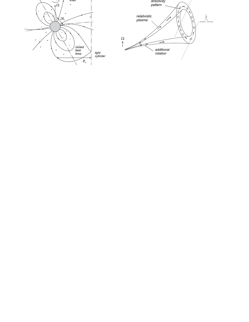
Figure 1: The main elements of the pulsar magnetosphere (a) and geometrical ’hollow cone’ model of the directivity pattern (b).

Indeed, it is clear that the rigid corotation becomes impossible at large distances from the rotation axis $r_{\perp}>R_{\rm L}$, where $R_{\rm L}=c/\Omega$ is so-called light cylinder radius (see Fig.1a). For ordinary pulsars $R_{\rm L}\sim$ $10^{9}$–$10^{10}$ cm, i.e., the light cylinder locates at the distances several thousand times larger than the neutron star radius. Further, we can estimate the polar cap size $R_{0}\approx(\Omega r/c)^{1/2}R$, i.e., the region at the magnetic pole of a neutron star, from which the magnetic field lines extend beyond the light cylinder. For ordinary radio pulsars the polar cap size is only several hundreds of meters. Importance of the polar cap region connects with the possibility for charged particles to escape from the neutron star magnetosphere. Indeed, as particles can move only along magnetic field lines (not only because of the smallness of the Larmor radius in comparison with another characteristic scales, but also due to very short synchrotron life time resulting in the drop to zero Landau level), two types of magnetic field lines appear in the magnetosphere. Open field lines start at the polar cap, smoothly intersect the light cylinder and extend to infinity. Closed field lines originate far from the magnetic axis and closed within the light cylinder. The plasma located on the closed magnetic lines is trapped, whereas the plasma filling the open magnetic lines can escape from the neutron star magnetosphere.

This simple model allowed V.Radhakrishnan & D.Cooke (and later L.Oster & W.Sieber) to formulate so-called ’hollow cone’ model of the pulsars radio emission, which perfectly accounted for their basic geometric properties. Indeed, the secondary plasma generation is to be suppressed in the very vicinity of the magnetic pole where, first, the intensity of the curvature radiation is low due to approx. rectilinear magnetic field lines and, second, the photons emitted by relativistic particles propagate at small angles to the magnetic field. Therefore, as shown in Fig.1b, in the central regions of the open magnetic field lines a decrease in the secondary plasma density should be expected. If we now make a rather reasonable assumption that the radio emission is directly connected with the outflowing plasma density, there must be a decrease in the radio emission intensity in the center of the directivity pattern. Therefore, without going into details (actually, the mean profiles have a rather complex structure), we should expect a single (one-hump) mean profile in pulsars in which the line of sight intersects the directivity pattern far from its center and the double (two-hump) profile for the central passage. This is exactly what is observed in reality.

In the same years three main parameters determining key physical electrodynamical processes were formulated

$$\rho_{\rm GJ}=-\frac{{\bf\Omega\cdot B}}{2\pi c},\qquad\lambda=\frac{n_{\rm e}}{n_{\rm GJ}},\qquad\sigma_{\rm M}=\frac{1}{4\lambda}\,\frac{eB_{0}\Omega^{2}R^{3}}{m_{\rm e}c^{4}}.$$ (2)

The first one is the charge density which is necessary to screen longitudinal electric field. This fundamental quantity introduced by P.Goldreich & P.Julian in 1969 determines also the characteristic number density $n_{\rm GJ}=|\rho_{\rm GJ}|/|e|$ (about $10^{12}$ cm^-3 near the star surface) and, what is much more important, characteristic current density $j_{\rm GJ}=c\rho_{\rm GJ}$. As it will be shown below, it is the electric current circulating in the pulsar magnetosphere that plays the main role in our play. The second parameter is the multiplicity $\lambda$ which shows to what extent the number density of the secondary plasma exceeds the critical number density $n_{\rm GJ}$. And the third one is so-called Michel magnetization parameter $\sigma_{\rm M}$. It corresponds to maximum bulk Lorentz-factor $\Gamma_{\rm max}$ which can be achieved if all the energy losses $W_{\rm tot}$ (1) transferred into bulk hydrodynamical particle flow ${\dot{N}}m_{\rm e}c^{2}\Gamma$, where ${\dot{N}}=\lambda\pi R_{0}^{2}n_{\rm GJ}c$ is the electron-positron ejection rate. Now the notation $\sigma=\sigma_{\rm M}/\Gamma=W_{\rm em}/W_{\rm part}$ is used, so we add subscript ’M’ for clearness.

Thus, in first several years after discovery of radio pulsars the answers to key questions were obtained. The only problem was in recognizing how does the pulsar magnetosphere work… Indeed, it was necessary to understand how the energy is transfeered from rotating neutron star to infinity, what is the energy spectrum of outflowing particles, and, certainly, what is the mechanism of the radio emission (which is to be coherent due to extremely high brightness tempetature up to $T_{\rm b}\sim 10^{28}$ K). Up to now the answers to most these questions remain unknown…

2.3 Rome (1973–1983)

Rome was the epoch when first strict laws were formulated. It concerned all main subjects including pair creation region, pulsar magnetosphere, and pulsar wind. At first, two detailed models of the pair creation in the vicinity of the neutron star surface were formulated. This process becomes possible due to continuous escape of particles along the open field lines. As a result, the domain (a ’gap’) with longitudinal electric field forms in the vicinity of the magnetic poles, its height being determined by the secondary plasma generation mechanism. As thought that time, a greater part of secondary particles is generated above the acceleration region, where the longitudinal electric field is rather small, so that the secondary plasma can freely escape from the neutron star magnetosphere.

First detailed model was developed in 1975 by M.Ruderman & P.Sutherland, and also by V.Eidman group. In their models the particle ejection from the neutron star surface plays no role as the electron work function was thought to be high enough. Later in 1978-1983, where more accurate theoretical consideration has shown that electron work function can be small, alternative model postulating free ejection of particles from the neutron star surface was developed by J.Arons group. It is the last model that was considered as the most adequate one within next three decades in spite of some intrinsic problems (e.g., in its first version it gave pair creation on the north half of the polar cap only).

The importance of these models was in determination of multiplicity $\lambda$ and the spectrum of secondary plasma. Starting from the first results obtained by J.Daugherty & A.Harding in 1982 it became clear that multiplicity cannot exceed $10^{4}$–$10^{5}$. This implies that the number density near the star surface $\lambda n_{\rm GJ}\sim 10^{16}$ cm^-3 is too low for detection 511 keV annihilation line. Accordingly, the Michel magnetization parameter $\sigma_{\rm M}$ is to be as large as $10^{3}$–$10^{4}$ for ordinary pulsars and can reach $10^{6}$ for fast young pulsars (Crab, Vela) only. As a result, the electron-positron injection rate ${\dot{N}}$ and the total injection $N=\int{\dot{N}}{\rm d}t$ per individual radio pulsar during all its life time can be presented as

$${\dot{N}}\approx\lambda\,\frac{B_{0}\Omega^{2}R^{3}}{ce}\sim 3\cdot 10^{34}\,P^{-2}B_{12}\,{\rm s}^{-1},\qquad N\approx\lambda\,\frac{Mc^{2}}{eB_{0}R}\sim 10^{50}\,B_{12}^{-1},$$ (3)

the last value depending very weak on initial period. As the total number of neutron stars in the Galaxy does not exceed $10^{9}$, one can conclude that radio pulsars cannot be the main sources of Galactic positrons. But pulsars may be relevant for PAMELA excess of energetic positrons in the energy domain 1–100 GeV, what is widely discussed now.

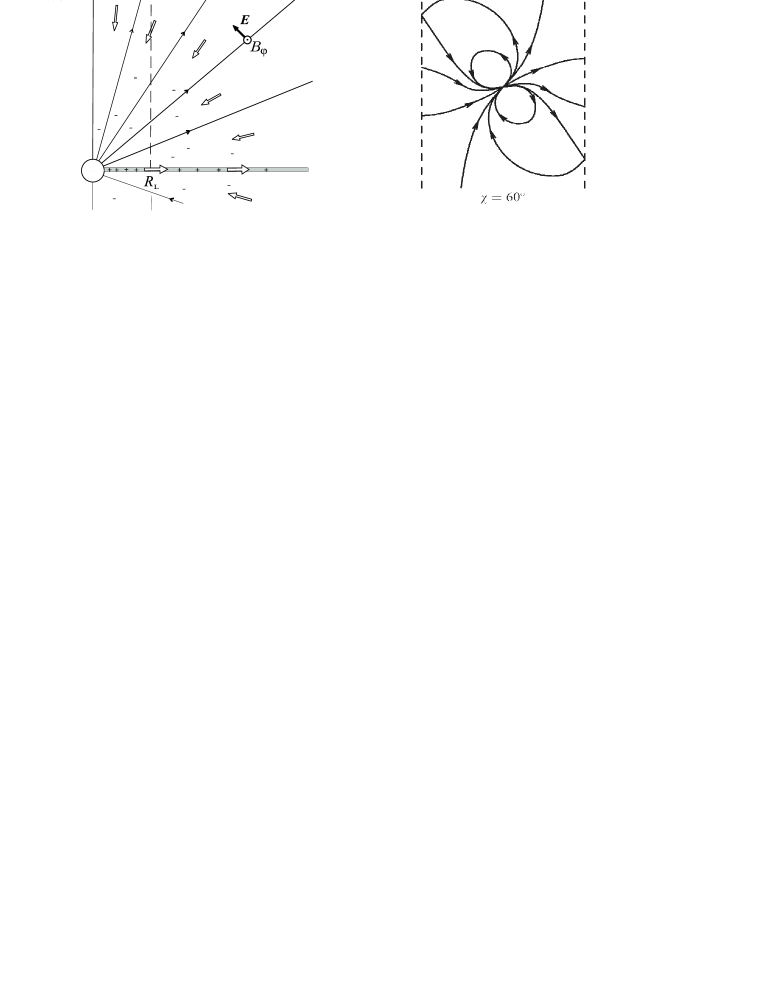
Figure 2: Michel split monopole solution (a) and BGI inclined solution with zero longitudinal electric current (b).

Important results were obtained in the theory of the pulsar magnetosphere and pulsar wind. First, L.Mestel, F.Michel, I.Okamoto and many other researchers formulated axisymmetric force-free ’pulsar equation’ which became the main instrument in theoretical consideration. In patricular, one of its analytical solutions (which could be found only for a few model profiles of the longitudinal current $j_{\parallel}$) have shown that for GJ longitudinal current $j_{\parallel}=j_{\rm GJ}$ one can construct quasi-spherical wind solution in which electric field is smaller than magnetic one up to infinity

$$B_{r}=B_{0}\frac{R^{2}}{r^{2}},\quad B_{\varphi}=E_{\theta}=-B_{0}\,\frac{\Omega R^{2}}{cr}\,\sin\theta,\quad j_{r}=\rho_{\rm GJ}c=-\frac{\Omega B_{0}}{2\pi}\,\frac{R^{2}}{r^{2}}\,\cos\theta,\quad S_{r}=\frac{B_{0}^{2}\Omega^{2}R^{4}}{4\pi cr^{2}}\sin^{2}\theta.$$ (4)

As shown in Fig.2a, in this solution longitudinal electric currents (contour arrows) generate toroidal magnetic field $B_{\varphi}$ which together with inductive electric field $E_{\theta}$ forms radial Poynting flux $S_{r}$ taking the energy away from a neutron star. Thus, the very possibility of the MHD outflow up to infinity was demonstrated. In such axisymmetric (i.e., time-independent) force-free solution all energy losses connect with the Poynting flux. But contrary to magneto-dipole wave, it is realised at zero frequency. Of course, the presence of the equatorial sheet separating outgoing in ingoing magnetic fluxes seemed rather artificial. But as we will see, this solution helped a lot in constructing self-consistent solution.

Besides, our team (V.Beskin, A.Gurevich & Ya.Istomin, hereafter BGI) have solved analytically the inclined version of the ’pulsar equation’ (see Fig.2b). It was found that for zero longitudinal electric current circulating in the neutron star magnetosphere the energy losses vanish for any inclination angle. This effect (confirmed later by L.Mestel group) results from full screening of the magneto-dipole radiation by magnetospheric plasma. This implies that the braking of the neutron star rotation results fully from impact of the torque ${\bf K}$ due to longitudinal currents circulating in the pulsar magnetosphere. It is convenient to describe two components of the torque ${\bf K}$ parallel and perpendicular to the magnetic dipole ${\bf m}$ by dimensionless current in the polar cap zone $i=j_{\parallel}/j_{\rm GJ}$ separating it into symmetric and antisymmetric contributions, $i_{\rm s}$ and $i_{\rm a}$, depending upon whether the direction of the current is the same in the north and south parts of the polar cap, or opposite. As one can easily check, $K_{\parallel}\propto i_{\rm s}$, and $K_{\perp}\propto i_{\rm a}$. Here and below we apply normalization to the ‘local’ Goldreich-Julian current density, $j_{\rm GJ}=|{\bf\Omega}\cdot{\bf B}|/2\pi$ (with scalar product). In particular, the direct action of the Ampère force on the star ${\bf K}=\int[{\bf r}\times[{\bf J}_{\rm s}\times{\bf B}]/c]\,{\rm d}{\bf S}$ by surface currents ${\bf J}_{\rm s}$ which close the longitudinal electric currents circulating in the pulsar magnetosphere can be written as

$$K_{\parallel}^{\rm sur}\approx-\frac{B_{0}^{2}\Omega^{3}R^{6}}{c^{3}}i_{\rm s},\quad K_{\perp}^{\rm sur}\approx-\frac{B_{0}^{2}\Omega^{3}R^{6}}{c^{3}}\left(\frac{\Omega R}{c}\right)i_{\rm a}.$$ (5)

In particular, for ‘local’ GJ current ($i_{\rm s}\approx i_{\rm a}\approx 1$) relations (5) imply $K_{\perp}^{\rm sur}\approx\left(\Omega R/c\right)K_{\parallel}^{\rm sur}$. Below we also assume (as was not done up to now) that the additional contribution for $K_{\perp}$ can give the magnetosphere itself, more precisely, the mismatch between magneto-dipole radiation from magnetized star and radiation generated by charges filling the pulsar magnetosphere (they exactly compensate themselves for $j_{\parallel}=0$). Here we write down $K_{\perp}^{\rm mag}$ in general form as

$$K_{\perp}^{\rm mag}=-A\,\frac{B_{0}^{2}\Omega^{3}R^{6}}{c^{3}}\,i_{\rm a}$$ (6)

trying to evaluate the dimensionless constant $A$ later from the results of numerical simulations.

Returning now to time evolution of the angular velocity $\Omega$ and the inclination angle $\chi$, one can write down

$$I_{\rm r}\,\dot{\Omega}=K_{\parallel}^{\rm A}+(K_{\perp}^{\rm A}-K_{\parallel}^{\rm A})\sin^{2}\chi,\quad I_{\rm r}\,\Omega\,{\dot{\chi}}=(K_{\perp}^{\rm A}-K_{\parallel}^{\rm A})\sin\chi\cos\chi,$$ (7)

where $I_{r}\sim MR^{2}$ is the neutron star momentum of inertia and we put $K_{\parallel}=K_{\parallel}^{\rm A}\cos\chi$ and $K_{\perp}=K_{\perp}^{\rm A}\sin\chi$. As both expressions contain the factor $(K_{\perp}^{\rm A}-K_{\parallel}^{\rm A})$, inclination angle $\chi$ is to evolve to $90^{\circ}$ (counter-alignment) if the total energy losses decrease for larger inclination angles, and to $0^{\circ}$ (alignment) if they increase with inclination angle. E.g., for local GJ longitudinal current ($i_{\rm s}^{A}\approx i_{\rm a}^{A}\approx 1$), as was supposed by BGI, we have counter-alignment evolution:

$$W_{\rm tot}^{({\rm BGI})}=i_{\rm a}^{\rm A}(\Omega)\,\frac{f_{\star}^{2}(\chi)}{4}\,\frac{B_{0}^{2}\Omega^{4}R^{6}}{c^{3}}\,\cos^{2}\chi,\quad{\dot{\chi}}^{({\rm BGI})}=i_{\rm a}^{\rm A}(\Omega)\,\frac{f_{\star}^{2}(\chi)}{4I_{\rm r}}\,\frac{B_{0}^{2}\Omega^{2}R^{6}}{c^{2}}\sin\chi\,\cos\chi,\quad 1.59<f_{\star}(\chi)<1.96.$$ (8)

Thus, during these years, it was able to formulate the basic laws of the pulsar magnetosphere. Moreover, several analytical solutions were constructed and even some quantitative predictions were formulated. It seemed that very soon we will understand the main properties of the magnetosphere of radio pulsars. Unfortunately, the problem was much more complicated. As a result, due to the lack of significant progress in the solution of nonlinear equations describing pulsar magnetosphere (which could not be solved analytically, and numerical methods have not yet been sufficiently developed) led to the abrupt decrease of a number of scientists working in this area. The dark ages came.

2.4 Dark ages (1983–1999)

Those were indeed dark ages, especially in the theory of the pulsar magnetosphere. At first glance, no results were obtained in that 15 years at all. But slowly, step by step, our understanding of the magnetospheric processes became more and more clear. First, important results were obtained in the theory of magnetized winds. Remember that force-free (i.e., massless) approach told nothing about the energy of outflowing particles. Only more general MHD theory, which was elaborated very intensively that time, demonstrated that in the quasi-spherical magnetized wind there is no effective particle acceleration. As was shown by A.Tomimatsu in 1994, at large distances (more exactly, outside the fast magnetosonic surface $r\gg r_{\rm F}$, where $r_{\rm F}\sim\sigma_{\rm M}^{1/3}\,R_{\rm L}$) particle energy cannot exceed $\sigma_{\rm M}^{1/3}\,m_{\rm e}c^{2}$, i.e., Poyting-to-particle energy flux ratio $\sigma=W_{\rm em}/W_{\rm part}$ is to be large: $\sigma\sim\sigma_{\rm M}^{2/3}\gg 1$. Simultaneously, it was recognized that the londitudinal electric current $j_{\parallel}$, as the accretion rate in Bondi accretion, is not a free parameter, but is to be fixed by crirical condition at the fast magnetosonic surface. In relativistic case it must be close to GJ current $j_{\rm GJ}$.

Another step ahead was connected with recognizing the importance of General Relativity (GR) in dynamics of the pair creation process. This effect results from additional term appearing in the expression for the GJ charge density $\rho_{\rm GJ}\approx-(\Omega-\omega)B/2\pi\,c$ connected with Lense-Thirring angular velocity $\omega$ . In spite of its smallness, appropriate derivative could be large enough. As was shown by V.Beskin in 1990 and by A.Muslimov & A.Tsygan in 1992, in Arons model the pair creation process becomes possible within all polar cap region just resulting from GR effects.

Besides, in the theory of the pulsar wind several very important results were obtained. At first, F.Coroniti and F.Michel have recognized that in the absence of the magneto-dipole wave the wind outflow from inclined magnetized neutron star is to contain ’striped’ current sheet separating ingoing and outgoing magnetic fluxes. Later C.Kennel & F.Coroniti analysing interaction of the pulsar wind with Crab nebula have found that at large distances compared with the dimension of the nebula the magnetization of the pulsar wind is to be very low: $\sigma\sim 10^{-2}$. It was in direct disagreement with theory prediction mentioned above. This ’$\sigma$-problem’, i.e., the impossibility to accelerate plasma effective enough in the quasi-radial pulsar wind, remains one of the main problem of the theory of the pulsar magnetopshere. At any way, within MHD approximation it cannot be solved.

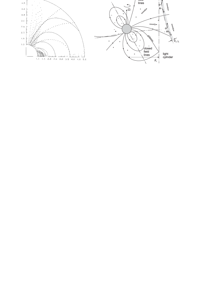
Figure 3: Two ’crazy’ ideas: Michel & Krause-Polstorff ’disk-dome’ structure of the pulsars magnetosphere (a) and BGI magnetospheric structure with light surface where very effective particle acceleration and current closure take place (b).

As often happens in difficult times, several ’crazy’ ideas were suggested (see Fig.3). First, F.Michel together with J.Krause-Polstorff in 1984-1985 has considered so-called ’disk-dome’ structure of the pulsar magnetosphere in which positive and negative charges are trapped in different regions of the magnetosphere, which are separated by vacuum region. At first glance, it was a step back in comparison with previuos works. In particular, it was unclear whether this configuration is stable in the presence of pair formation or not. But, as we will see, this structure was reproduced in recent numerical simulations.

Besides, BGI group considered the case where longitudinal current $j_{\parallel}$ is small enough so that MHD flow cannot be realized up to infinity. In this case, as is also shown in Fig.3, the magnetosphere has a ’natural boundary’ — the light surface, where electri field becomes equal to magnetic one, and where very effective bulk particle acceleration up to $\Gamma\approx\sigma_{\rm M}$ takes place (solving the $\sigma$-problem!); as we shall see, this assumption also subsequently found its indirect confirmation. This structure inevitably appears for the inclined rotator and for Arons model, which postulated exactly local GJ longitudinal current density $j_{\parallel}=c\rho_{\rm GJ}\approx\Omega B\cos\chi/2\pi$, i.e., the current which is small enough to support MHD outflow to infinity. Indeed, as was shown above, in MHD wind the toroidal magnetic field at the light cylinder is to be equal to electric one. But for local GJ electric current (and for inclined rotator) the total current is too small to generate large enough toroidal magnetic field. Thus, within BGI model the low-$\sigma$ pulsar wind is formed already in the vicinity of the light cylinder.

2.5 Renaissance (1999–2006)

This epoch (started with two papers published in 1999) was the time of rapid breakthrough in understanding the beauty and the truth. In the first one I.Contopoulos, D.Kazanas & Ch.Fendt (CKF) found numerically (by the iterative procedure) the solution of the axisymmetric ’pulsar equation’. Similarly to Michel split-monopole solution, at large distances $r>R_{\rm L}$ it contained the equatorial current sheet, but near the stellar surface it corresponded to dipolar, not monopolar magnetic field (see Fig.4a). In a few years this structure was reproduced in many papers rebooting the interest to the theory of the pulsar magnetosphere. Or course, these solutions concerned axisymmetric structure which gave us no information about real time-dependent magnetospheres of radio pulsars.

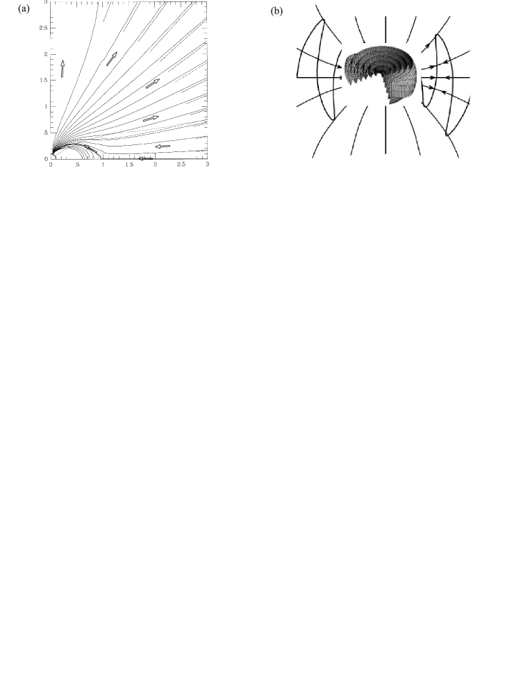
Figure 4: CKF axisymmetric force-free pulsar magnetosphere; contour arrows show electric currents (a) and Bogovalov ’incline split monopole’ analytical solution (b).

Simultaneously, S.Bogovalov found analytical force-free solution for ’inclined split monopole’ pulsar wind

$$B_{r}=B_{0}\frac{R^{2}}{r^{2}}\,{\rm Sign}(\Phi),\,B_{\varphi}=E_{\theta}=-B_{0}\,\frac{\Omega R^{2}}{cr}\,\sin\theta\,{\rm Sign}(\Phi),\,\Phi=\cos\theta\cos\chi-\sin\theta\sin\chi\cos\left[\varphi-\Omega\left(t-r/c\right)\right],$$ (9)

where the condition $\Phi=0$ just determines the shape of the striped current sheet (see Fig.4b). On the other hand, near the star the magnetic field had monopolar structure. In this solution within the cones $\theta<\pi/2-\chi$, $\pi-\theta<\pi/2-\chi$ around the rotation axis the electromagnetic fields are time-stationary and coinside with axisymmetric Michel solution, which was already shown in Fig.2a. On the other hand, in the equatorial region all components of electromagnetic field change signs at the instant when the current sheet intersects given point; between these intersection times the fields remain time-independent. It is not superfluous to mention that this solution contained no magneto-dipole wave. It is necessary to stress as well that the condition $\Phi=0$ for the shape of the current sheet actually has the kinematic origin. In particular, it is to be true for any solution with radial poloidal field lines and asymptotic behavior $E_{\theta}(\theta)=B_{\varphi}(\theta)$ with arbitrary $\theta$-dependence as well; such time-indepenent asymptotic solution of the ’pulsar equation’ was analytically obtained by R.Inhragam already in 1973. So, it is not surprising that later the shape of the striped current sheet was reproduced in all numerical simulations.

Thus, undeniable progress has been made during these years. At first, it was in recognizing the extremely important role of the current sheet in the dynamics of the pulsar wind. It is not surprising that analysis of physical processes inside the current sheet became the mainstream in the pulsar wind theory. In particular, J.Kirk & Yu.Lyubarsky have mentioned the role of magnetic reconnection, which also gave start to numerous investigations. Another key point was connected with the determination of ’universal solution’ which, as was already stressed, was reproduced in many papers. But the most important subject was in changing the very sight on the londitudinal current circulating in the pulsar magnetosphere. Longitudinal current $j_{\parallel}^{({\rm us)}}$ given by ’universal solution’, not by the pair creation mechanism was decleared now as the correct value corresponding to the real configuration. In other words, it was postulated that the solution with zero longitudinal electric field (both force-free and MHD approaches deny that) must satisfy not only the electric charge condition $\rho_{\rm e}=\rho_{\rm GJ}$, but also the current conition $j_{\parallel}=j_{\parallel}^{({\rm us)}}$. For this reason, no restriction on the longitudinal electric current was postulated within all force-free and MHD simulations; in the last case plasma was freely injected into domains, where during the simulation the plasma number density becomes low enough.

On the other hand, some points were not clarified. At first, ’universal solution’ gave the profile of longitudinal current density $j_{\parallel}$ which was in direct disagreement with Arons model postulating, as was specially stressed above, local GJ current density. Simultaneously, it contradicted ’split monopole’ profile as well. In particular, as shown in Fig.4a, ’universal solution’ predicted volume return current. Remember that common point of view in first papers devoted to pulsar magnetosphere was in introducing return electric current only along the separatrix separating open and closed magnetic field lines. Indeed, all pair creation models postulated the same sign of the accelerating potential difference through the polar cap for non-orthogonal rotators and, accordingly, the same direction of the longitudinal current. Appearence of the volume return current through the polar cap area was rather strange as it was in a direct disagreement with the pair creation models. Though this difficulty has not been spoken aloud, first attempts were made to resolve this contradiction already at that time. In particular, S.Shibata and later A.Beloborodov demonstrated that on field lines with small enough longitudinal current $j_{\parallel}<j_{\rm GJ}$, particle acceleration and the pair creation in the polar cap process is to be supressed.

2.6 Industrial revolution (2006–2013)

Industrial revolution in pulsar physics was connected with the possibility to produce 3D time-dependent simulations; as any revolution, it succeeded in resolving accumulated intrinsic problems by purely technical means. This epoch started with a paper published in 2006 in which A.Spitkovsky numerically solved force-free equations for inclined rotator. It was the first 3D solution for rotating inclined magnetic dipole with the wind extending up to infinity. As shown in Fig.5a, in spite of small computation box, this solution confirmed the existence of the striped current sheet.

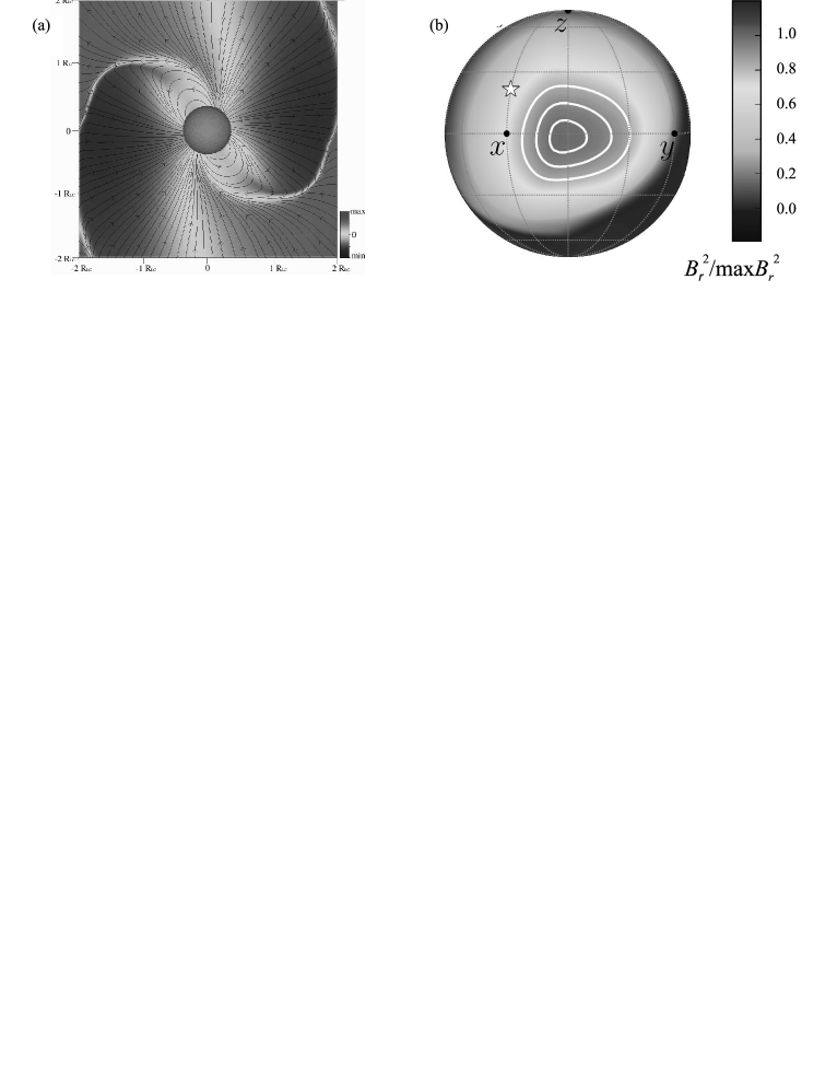
Figure 5: Inclined ($\chi=60^{\circ}$) Spitkovsky force-free solution (a) and MHD solution demonstrating concentration of magnetic field lines at $r=6\,R_{\rm L}$ in the direction shifted in azimuth by about $30^{\circ}$ to magnetic axis (contour star) (b).

Industrial revolution is impossible in one separate country. After this paper, not only force-free, but also MHD simulations for inclined rotator were produced in many scientific centers. As a result, ’universal inclined solution’ was found. In particular, the original result obtained by A.Spitkovsky for total energy losses

$$W_{\rm tot}^{({\rm MHD})}\approx\frac{1}{4}\,\frac{B_{0}^{2}\Omega^{4}R^{6}}{c^{3}}\,(1+\sin^{2}\chi),\quad{\dot{\chi}}^{({\rm MHD})}\approx-\frac{1}{4I_{\rm r}}\frac{B_{0}^{2}\Omega^{2}R^{6}}{c^{2}}\sin\chi\,\cos\chi$$ (10)

was confirmed. As we see, ’universal solution’ gives the increase of total energy losses with inclination angle $\chi$, and, according to Eqn. (7), its aligned evolution (the second expression confirmed this point was obtained later).

On the other hand, it was shown that ’universal solution’ differs drastically from the Michel-Bogovalov split-monopole one (9). In particular, for large enough inclination angles $\chi>30^{\circ}$ the radial magnetic field is compressed to equatorial plane, so that approximately

$$<B_{r}>_{\varphi}\approx B_{0}\frac{R^{2}}{r^{2}}\,\sin\theta\,{\rm Sign}(\Phi),\quad<B_{\varphi}>_{\varphi}=<E_{\theta}>_{\varphi}\approx-B_{0}\,\frac{\Omega R^{2}}{cr}\,\sin^{2}\theta\,{\rm Sign}(\Phi),\quad<S_{r}>_{\varphi}\approx\frac{B_{0}^{2}\Omega^{2}R^{4}}{4\pi cr^{2}}\sin^{4}\theta,$$ (11)

while Michel-Bogovalov solution (9) corresponds to homogeneous radial magnetic field $B_{r}=B_{0}(R^{2}/r^{2})\,{\rm Sign}(\Phi)$. As was already stressed, radial asymptotic solutions with arbitrary $\theta$-dependenses were known since 70-ties. But it was surprising that the results of 3D time-dependent MHD simulation (11) are in good agreement with very simple force-free solution predicting, e.g., the general connection $S_{r}(\theta)\propto B_{r}^{2}(\theta)\,\sin^{2}\theta$, which is just fulfilled. Besides, it turned out that appropriate dimensionless current $i_{\rm a}^{\rm A}\sim(\Omega R/c)^{-1/2}$ is insufficient to explain MHD energy losses (10) only by the Ampére force torque $K^{\rm sur}$ (5) due to polar cap surface currents. Evidently, they can be connected with magnetospheric losses (6) if we assume $A\sim(\Omega R/c)^{1/2}$. It is important that for such a value $A\ll 1$ on can neglect the contribution of the magnetospheric torque $K_{\perp}^{\rm mag}$ (6) within BGI model (8), as was actually done.

One can stress here that in Eqn. (11) $\varphi$-averaged values are presented. In reality, as shown in Fig.5b, there is visible concentration of magnetic field lines (as well as the Poynting flux) in direction shifted in azimuth by about $30^{\circ}$ to magnetic axis (contour star); in other words, in the equatorial region between two parts of the current sheet the flow is $\varphi$-dependent. In this point there is another very important difference with Michel-Bogovalov solution in which, as is clear from Eqn. (9), the electromagnetic fields are not time- and $\varphi$-depenent outside the striped current sheet.

At the same time, new sight on the universal current structure allowed A.Timokhin (and later A.Timokhin & J.Arons) to consider in more detail the pair creation region in the vicinity of the magnetic poles. Now longitudinal current $j_{\parallel}^{({\rm us)}}$ was the input parameter in their consideration. It was demonstrated that pair creation is indeed possible for large enough longitudinal currents $j_{\parallel}>j_{\rm GJ}$ and, as was already mentioned, not possible for smaller ones. Moreover, it was shown that pair creation is possible for volume return current as well. It becomes possible due to essential time-dependence of the pair creation process. Unfortunately, these were 1D simulations which could potentially loose some important features. In particular, it was impossible to include into consideration the time-dependence of the toroidal magnetic field. Nevertheless, this work was very important in understanding the very possibility to produce longitudinal current which differs drastically from local GJ current. And one of the main result was associated with an actual return to RS model in which particle injection from the star surface does not play a determining role.

To summarize, one can conclude that industrial revolution helped us to make the next step in understanding the structure of the pulsar magnetosphere. It is very important that all these results were confirmed by several groups independently. Nevertheless, some key problems were not solved. And the main one concerned the support of the necessary current $j_{\parallel}^{({\rm us)}}$, which was determined by ’universal solution’, by pair creation processes in the magnetosphere.

2.7 Modern time (2014–)

Formally, it was only the next step in numerical simulation associated with 3D particle-in-cell (PIC) code. But actually it was a qualitative step ahead as only kinetic treatment, unlike force-free and MHD approaches, could self-consistently include into consideration the pair creation process, i.e., the acceleration regions with nonzero parallel electric field $E_{\parallel}$ and subsequent particle injection into the computation domain. In other words, PIC approach, at least in principle, allows to produce ab-initio simulations. Of course, this epoch is in the very begining, so not all results presented below were confirmed by independent consideration. Besides, in spite of (natural for this stage) childhood diseases, new possibilities connected with PIC approach have already given a number of very interesting results.

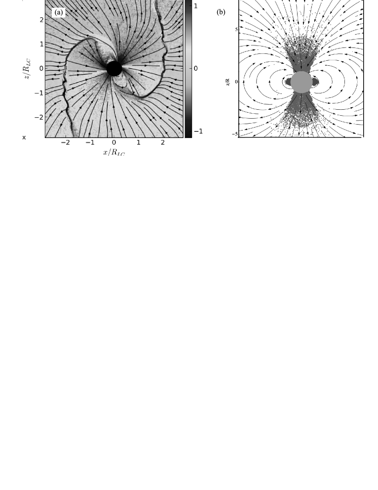
Figure 6: First Princeton PIC simulations: solution for incline rotator (a) and for axisymmetric case without including GR effects into consideration (b).

At first, as shown in Fig.6a, A.Philippov, A.Spitkovsky & B.Cerutti have reproduced MHD structure contaning, in particular, striped current sheet. These simulation also provided extra confirmation of the existence of the ’universal solution’. Second, the possibility of the effective particle acceleration just outside the light cylinder up to $\Gamma\approx\sigma_{\rm M}$ was demonstrated as well. This process became possible due to the appearence of a domain with high enough electric field $E>B$ inside the equatorial current sheet. In addition, reconnection electric field even in the axisymmetric case helps particles to drift towards the current sheet. As a result, up to 30% of the electromagnetic energy flux dissipates in the vicinity of the light cylinder $r<5\,R_{\rm L}$ transferring electromagnetic energy flux into particle acceleration. At the moment it is rather difficult to say whether this process solves the $\sigma$-problem (it is definitely not at 5 light cylinders), but, certainly, some step ahead was done. At any way, such an effective particle acceleration definitely helps us to explain high energy radiation detected by Fermi observatory.

On the other hand, in some sense PIC simulations have put more questions than give answers. Indeed, already the first results obtained by A.Philippov & A.Spitkovsky and by A.Chen & A.Beloborodov in 2014 for axisymmetric magnetosphere have suddenly shown the absence of pair creation in polar region near magnetic poles. In contrast, as one can see in Fig.6b, free ejection from the neutron star surface (which was postulated in their work) resulted in the formation of the ’disk-dome’ structure which was already discussed above. Later it was shown that pair creation in the bulk of the polar cap is absent in the inclined magnetosphere for small enough inclinations $\chi<30^{\circ}$. This effect was connected with a little bit smaller longitudinal current $j_{\parallel}^{({\rm us})}$ in comparison with $j_{\rm GJ}$; as was already stressed, in this case no particle acceleration and pair creation takes place. Fortunately, this problem was soon resolved. It turned out that GR effects (which, as was already mentioned, changes the GJ charge density) flips the inequality to $j_{\parallel}^{({\rm us})}>j_{\rm GJ}$ allowing thereby the pair creation process. As is shown in Fig.6a, in this case PIC simulation reproduced in general the structure obtained within MHD approach.

The second, more serious problem concerned the formation of the return current. At the moment, the authors succeeded in effective closing of the currrent only for fast pulsars when electromagnetic fields and particle number density near the light cylinder are high enough, so that pair creation process takes place there. In other words, at the moment it is impossible to close electric current without additional pair creation region close to the $Y$-point. On the contrary, A.Chen & A.Beloborodov and A.Philippov & A.Spitkovsky have found the solutions close to the disk-dome structure in the case when outer magnetosphere pair production was suppressed.

3 CONCLUSION

Thus, now the theory of the pulsar magnetosphere and pulsar wind is a rapidly evolving field accumulating in the last years tens of researchers. Real progress was achieved including some quantitative predictions (e.g., the expressions for energy losses) which, as one might expect, can be directly checked. Unfortunately, pulsars give us no pure experiment, and the quantitative predictions are usually hidden in observations. E.g., up to now we have not identified the direction of the inclination angle evolution ${\dot{\chi}}$. Another observable parameter, i.e., so-called ’braking index’ $n_{\rm br}={\ddot{\Omega}}\Omega/{\dot{\Omega}}^{2}$ also cannot be directly used for the analysis of the pulsar evolution as there are additional fluctuations of the value ${\ddot{\Omega}}$ (most likely, due to precession of neutron star, which has non-spherical shape) on the time scale much smaller than the dynamical life time $\tau_{\rm D}\sim P/{\dot{P}}$. For this reason, for most pulsars observations give unrealistic values $n_{\rm br}=\pm(10^{4}$–$10^{5})$. As a result, only for a few fast young pulsars their braking indexes can be used for the analysis of their energy losses.

Table 1: Braking indexes $n_{\rm br}={\ddot{\Omega}}\Omega/{\dot{\Omega}}^{2}$ for fast radio pulsars (from Archibald et al, ApJ, 819, L16, 2016)

J1734+3333	B0833-45	J1833-1034	B0540-69	B0531+21	B1509-59	J1640-4631
0.9(2)	1.4(2)	1.857(1)	2.14(1)	2.51(1)	2.839(1)	3.15(3)

As shown in Table 1, for most young pulsars observations give $n_{\rm br}\sim 3$, which in zeroth approximation does not contradict theoretical predictions (below I do not include possible evolution of the magnetic field into consideration)

$$n_{\rm br}^{({\rm V)}}=3+2\cot^{2}\chi,\qquad n_{\rm br}^{({\rm BGI})}=1.93+1.5\,\tan^{2}\chi,\qquad n_{\rm br}^{({\rm MHD})}=3+\frac{\sin^{2}\chi\,\cos^{2}\chi}{(1+\sin^{2}\chi)^{2}}.$$ (12)

On the other hand, in order to extract the evolution law from observations it is necessary to determine braking index $n_{\rm br}$ up to the second digit simultaneously avoiding any additional disturbances. That is impossible at the moment. Indeed, most of young pulsars have $n_{\rm br}<3$, in good agreement with BGI results. On the other hand, ’universal MHD’ model predicts $3<n_{\rm br}<3.25$. But it only implies that additional precession is to be included into consideration to match theoretical predictions with observations. Long-term observations are necessary to clarify this point. Until then BGI model (with low-$\sigma$ pulsar wind and the absence of striped current sheet) remains afloat.

4 ACKNOWLEDGMENTS

I thank A.Beloborodov, J.Petri and A.Philippov for very instructive discussions. This research was supported by Basic Research Program P-7 of the Presidium of the Russian Academy of Sciences.