Notes on the computation of periodic orbits using Newton and Melnikov’s method

1 Introduction

The main goal of these sessions will be to understand the dynamics of a system exhibiting a continuum of periodic orbits when we add a small periodic forcing. The most paradigmatic example is probably the perturbed pendulum; however, such systems massively appear in real applications, specially in celestial mechanics. This has given rise to classical problems exhibiting extremely rich dynamics, such as the restricted three body problem.

In these sessions we will see some theoretical results, but we will mainly visualize them through analytical and numerical computations for a particular example, the forced pendulum:

$$\ddot{u}+\sin(u)=\varepsilon g(x,t),$$ (1)

where $\varepsilon\geq 0$ is a small parameter, $x=(u,\dot{u})$ and $g(x,t)$ a periodic forcing: $g(x,t+T)=g(x,t)$.

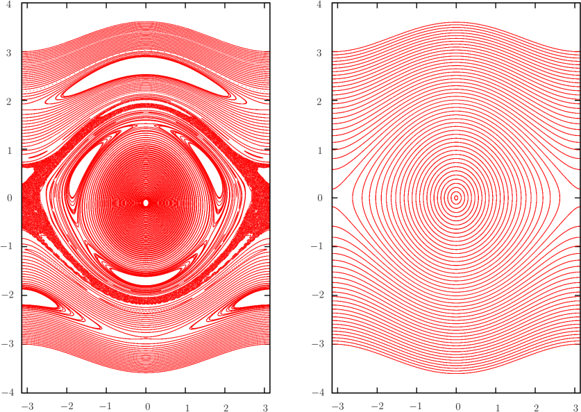
Figure 1: Phase portrait of the unperturbed pendulum (right). Phase portrait for $\varepsilon>0$ (left).

We will mainly see that, when $\varepsilon=0$ the face portrait looks like Figure 1 (right) and that, when $\varepsilon>0$ looks like Figure 1 (left). We will learn theoretical and numerical techniques to compute the surviving resonant periodic orbits (large “holes” in Figure 1 left).
Although everything we will see will be generic for any $g(x,t)$, we will fix this forcing from now on say to

$$g(x,t)=\sin(\omega t),$$

ant $T$ becomes $T=\frac{2\pi}{\omega}$.
It will be useful to write the system as a first order one by increasing the dimension. Let $v=\dot{u}$, then we can write it as

$$\left\{\begin{aligned} \dot{u}&=v\\ \dot{v}&=-\sin(u)+\varepsilon\sin(\omega t).\end{aligned}\right.$$ (2)

2 Dynamics of the pendulum around the elliptic point

2.1 Unperturbed phase portrait

We will start with some exercises in order to understand the dynamics of the unperturbed pendulum ($\varepsilon=0$).

Exercise 1.

Consider the unperturbed equations of the pendulum by setting $\varepsilon=0$ in Eq. (2):

$$\left\{\begin{aligned} \dot{u}&=v\\ \dot{v}&=-\sin(u)\end{aligned}\right.$$ (3)

1. Obtain the equilibrium points and state their type.

2. Obtain a Hamiltonian for system (3).

Solution 1.

1. The system possesses an elliptic equilibrium point at the origin and two saddle points at $(\pm\pi,0)$.

2. The function

   $$H(u,v)=\frac{v^{2}}{2}-\cos(u)$$

   is the Hamiltonian of system (3) up to a constant value.

Exercise 2.

Write a small program in Matlab to plot the phase portrait of system (3).

Solution 2.

The phase portrait for the unperturbed pendulum looks like the one in Figure 1 (right). The phase portrait is divided in two regions by two separatrices. These separatrices are given by two homoclinic trajectories connecting the two saddle points, and are located at the level of energy $H(u,v)=\frac{0^{2}}{2}-\cos(\pi)=1$. In the inner part we find the elliptic equilibrium point, which is surrounded by a continuum of periodic orbits. Provided that the energy level of the elliptic point is $H(0,0)=-1$, each periodic orbit is located a certain level of energy between $1$ and $-1$: $H(u,v)=c$, $c\in(-1,1)$. Outside the homoclinic loop we also find a continuum of periodic orbits, given by $H(u,v)=c$, $c>1$.

From now on we will focus on what happens with the periodic orbits inside the homoclinic loop when we add a small periodic forcing to System (3) (say $\sin(\omega t)$). To this end, it will be crucial to compute the periods of the periodic orbits for $\varepsilon=0$. Let’s us now see a general theoretical approach to obtain a formula.

Assume we have Hamiltonian system of the form

$$H(u,v)=\frac{v^{2}}{2}+V(u),$$

where $V(u)$ is a potential energy. Assume that we have a periodic orbit at level of energy $c\in\mathbb{R}$ given by $H(u,v)=c$. Then, we can compute its period, $T_{c}$, as follows:

$$T_{c} =\oint_{H(u,v)=c}dt=\oint_{H(u,v)=c}\frac{1}{\frac{du}{dt}}du$$

$$=\oint_{H(u,v)=c}\frac{1}{\dot{u}}du.$$

using that the system is Hamiltonian and, hence, $\dot{u}=\frac{\partial H(u,v)}{\partial v}=v$ we get

$$T_{c}=\oint_{H(u,v)=c}\frac{1}{v}du.$$

Isolating $v$ from $H(u,v)=c$,

$$T_{c}=\oint_{H(u,v)=c}\frac{1}{\sqrt{2(c-V(u))}}du.$$

But now we have two problems. First, solving such an integral explicitly can be a nightmare, if possible at all. Second, doing integrals numerically is a difficult task, it’s slow and imprecise. Moreover, note that, although the integral converges, the integrand has an asymptote at the crossing point with the horizontal axis: $(0,u_{1})$ such that $V(u_{1})=c$. This is specially problematic when computing this integral numerically.
Fortunately, there is an alternative: compute a Poincaré map using a transversal section to the periodic orbit and capture the return time.

Exercise 3.

Write a small program in Matlab to compute the periods of the periodic orbits using the Poincaré map from the section $\left\{u=0\right\}$ to itself.

Solution 3.

Use the function period.m to obtain something similar to Figure 2. Note that, the argument of this function is $v_{0}$ and starts integrating at $(0,v_{0})$. Hence, the corresponding level of energy becomes $H(0,v_{0})=\frac{v_{0}^{2}}{2}-1$.
Note that there is a vertical asymptote at $c=1$, which corresponds to the energy level of the homoclinic loop.

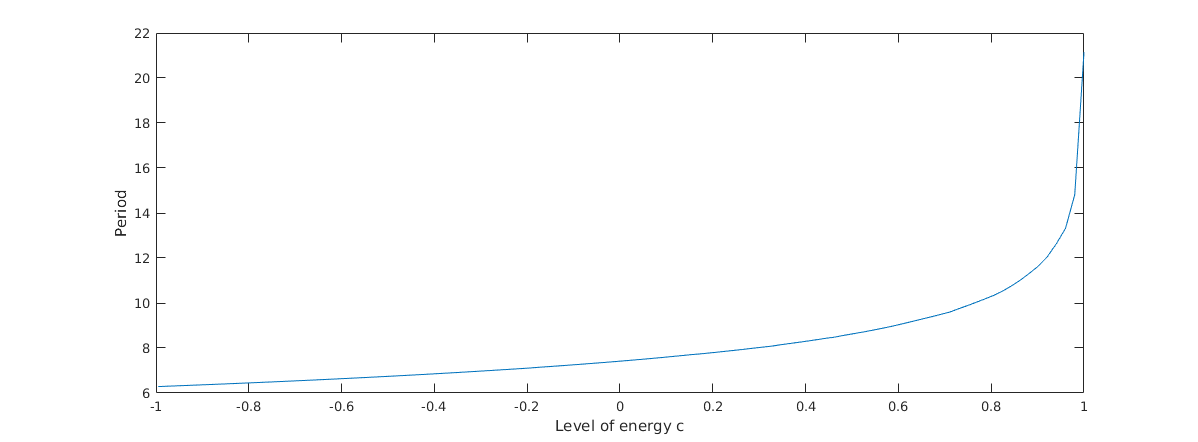
Figure 2: Periods of the periodic orbits for the unperturbed pendulum.

2.2 Stroboscopic vs Poincaré map

In general, for autonomous systems, in order to study the existence of periodic orbits one typically considers a Poincaré map:

$$P:\Sigma:\longrightarrow\Sigma,$$

where $\Sigma$ is a co-dimension one section transversal to the periodic orbits. In our case, we could take the vertical axis $\Sigma=\left\{(u,v)\,|\,u=0\right\}$. Then, fixed points of the Poincaré map, points $x_{0}\in\Sigma$ such that $P(x_{0})=x_{0}$, become initial conditions for periodic orbits for the flow, whose period is the flying time. Periodic points of the Poincaré map, $P^{n}(x_{0})=x_{0}$, also give rise to periodic orbits for the flow, which cross $n$ times the Poincaré section and their period becomes the addition of all flying times between consecutive impacts with the Poincaré section before $x_{0}$ is reached again.
However, if the system is not autonomous (but periodic), then one needs to take into account the initial time and consider Poincaré sections of the form $\Sigma\times\mathbb{T}_{T}$, with $\mathbb{T}_{T}=\mathbb{R}/T\mathbb{Z}$. Then, a sufficient condition for the existence of a periodic orbits becomes $P^{n}(x_{0},t_{0})=(x_{0},t_{0}+mT)$. That is, after the point $x_{0}$ is reached again after $n$ crossings and the total spent time is a multiple of $T$. Then, the flow possesses an $mT$-periodic orbit crossing the section $n$ times. Note that, if total time spent to reach $x_{0}$ again is not a multiple of $T$, then nothing can be said about the existence of a periodic orbit.

One of inconveniences of using Poincaré maps with non-autonomous systems is the need of computing the flying time. Although this can be done numerically, it requires extra computations than simply numerically integrating a flow, as one needs to compute the crossing with the section. Alternatively, one can use the stroboscopic map, which consists of integrating the system for a time $T$:

$$\begin{array}[]{cccc}s_{\varepsilon}:&\Sigma_{t_{0}}&\longrightarrow&\Sigma_{t_{0}}\\ &x&\longmapsto&\varphi_{\varepsilon}(T;x,t_{0}),\end{array}$$ (4)

where

$$\Sigma_{t_{0}}=\left\{(x,t)\in\mathbb{R}^{2}\times\mathbb{T}_{T}\right\},\,\mathbb{T}_{T}:=\mathbb{R}/T\mathbb{Z}.$$

Then, if $s_{\varepsilon}^{m}(x_{0})=x_{0}$, then $x_{0}$ is the initial condition for a $mT$-periodic orbit:

$$s_{\varepsilon}^{m}(x_{0})=\varphi_{\varepsilon}(t_{0}+mT;x_{0},t_{0})=x_{0}.$$

Exercise 4.

Use the Matlab script iter_strobo.m or iter_strobo_parallel.m to simulate the stroboscopic map for a set of different initial conditions. The latter parallelizes the loop and is faster if you have more cores available.

2.3 Dynamics of the stroboscopic map: unperturbed case

As mentioned above, for $\varepsilon=0$, System (2) possesses a continuum of periodic orbits surrounding the origin and whose periods increase when approaching the homoclinic loop. Therefore, when picking up a point, all its iterates will be located in an invariant curve, which is nothing else than the periodic orbit of the time-continuous system. However, the dynamics of the map will exhibit different properties depending on the relation between $T$ and $T_{c}$.
Imagine we iterate a point $x_{0}=(u_{0},v_{0})$ such that $H(x_{0})=c\in(-1,1)$. Then, if $T$ and $T_{c}$ are congruent ($T$ and $T_{c}$ are rational multiples), this point will be a periodic point of the stroboscopic map. Let us assume that there exists some $m\in\mathbb{Z}$ such that $T_{c}=mT$. Then, the stroboscopic map will return to $x_{0}$ after $m$ iterates:

$$s_{0}^{m}(x_{0})=x_{0}.$$

Indeed, all points at the level of energy $c$ will be $m$-periodic points

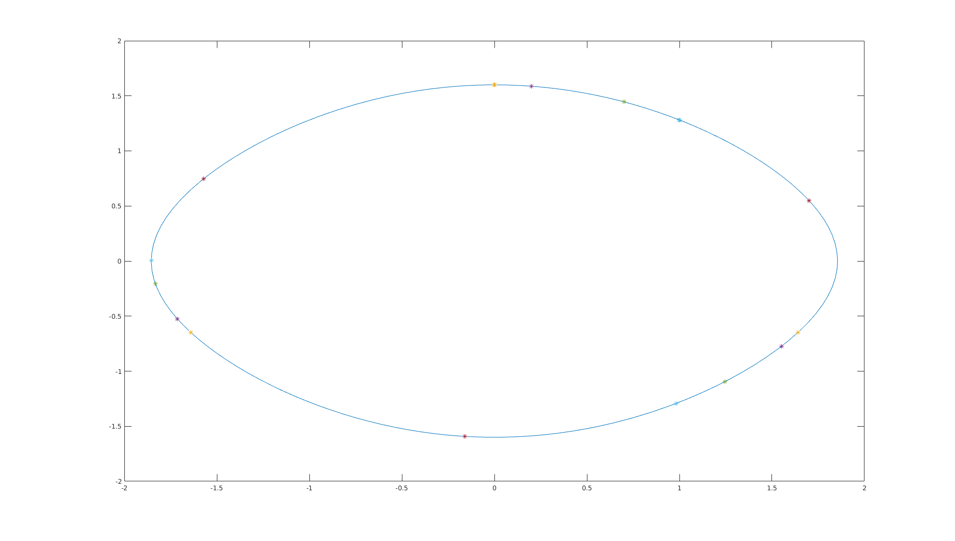
Figure 3: Continuous curve: periodic orbit with period $T_{c}=3T$. Points: different initial conditions (with different colors) and its iterates.

of the stroboscopic map. This is illustrated in Figure 3 we show a periodic orbit with $T_{c}=3T$ and the iterates of different initial conditions taken at this trajectory. Note that they all form a $3$-periodic orbit: for any $x_{0}$ at that level of energy we have $s_{0}^{3}(x_{0})=x_{0}$. The parameters have been bound as follows. We have chosen an arbitrary level of energy $H(0,1.6)=c$. Then, using the function period.m, we have found the period of this level set, $T_{c}$, and then chosen $T$ such that

$$T_{c}=3T.$$

Note that, this relation imposes the fact that, after iterating $3$ times the stroboscopic map, the time-continuous system has performed exactly one loop. However, let us see what happens if we choose $T$ such that $T_{c}=\frac{mT}{n}$.

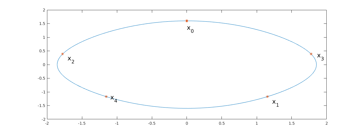
Figure 4: Continuous curve: periodic orbit with period $T_{c}=\frac{2T}{5}$. Red points: iterates of the point $(0,v_{0})$ such that $H(0,v_{0})=c$ and $T_{c}=\frac{2T}{5}$.

In Figure 4 we show the situation at the same level of energy when choosing $T$ such that $T_{c}=\frac{2T}{5}$. In this case we only show the iterates of a unique point at that level energy, but all points have the same behaviour. Note that, in this case, the points are not ordered with increasing angle, but at each iteration one skips one point ($s(x_{i})=x_{i+1}$). Therefore, when the loop is closed, we have twisted twice along the periodic orbit of the time continuous system. This is called a subharmonic orbit and one says that has rotation number $\frac{2}{5}$. Roughly speaking, the rotation number of a periodic orbit measures the average angle twisted at each iterate. Note that, in the previous example, one has a harmonic periodic orbit with rotation number $\frac{1}{3}$.

Summarizing we have the following fact.

Fact 1.

If $T$ is such that $T_{c}=\frac{mT}{n}$, then all points satisfying $H(x_{0})=c$ are $m$ periodic points of the stroboscopic map:

$$s_{0}^{m}(x_{0})=x_{0}.$$

When the cycle is closed, the iterates have performed $n$ loops around the origin. In other words, the rotation number of the periodic orbit is $n/m$.

Let us now discuss the situation when $T$ and $T_{c}$ are incommensurable (such $m$ and $n$ do not exist). Recalling that the time-continuous system is $T$-periodic, any periodic orbit needs to spend a time multiple of $T$ to close. If there doesn’t exist any integer combination such that $nT_{c}=mT$, then any point at the level of energy $H(u,v)=c$ cannot be closed by iterating the stroboscopic map. To see that, let us assume that $s_{0}^{m}(x_{0})=x_{0}$ for some $m$. Then there is a point satisfying $H(x_{0})=c$ such that

$$\varphi_{0}(mT;x_{0})=x_{0}.$$

On the other hand, we also have that $\varphi_{0}(T_{c};x_{0})=x_{0}$ and, therefore, $T_{c}=mT$, which is a contradiction, and the point never returns to itself when iterated by the stroboscopic map.
As a consequence, as the periodic orbit is an invariant curve for the stroboscopic map, when iterating the map we will densely fill this curve. In theory, if the map restricted to the invariant curve is not $C^{2}$, this can lead to a Denjoy counterexample (see [Nit71]) and one could get a Cantor set instead of filling this curve densely.

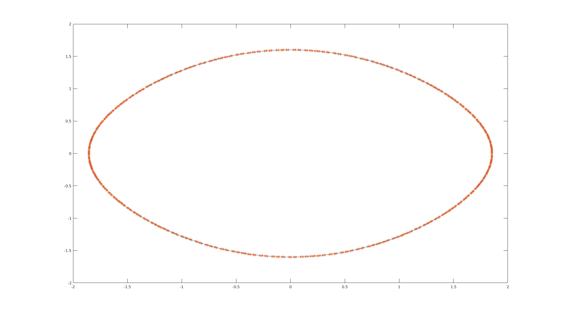
Figure 5: Blue curve: periodic orbit with period $T_{c}=\frac{T}{\sqrt{2}}$. Red points: $500$ iterates of the point $(0,v_{0})$ such that $H(0,v_{0})=c$ and $T_{c}=\frac{T}{\sqrt{2}}$.

In Figure we show the iterates of a point belonging at the level of energy $H(0,1.6)=c$ with $T_{c}=\frac{T}{\sqrt{2}}$.

Remark 1.

For $\varepsilon=0$ the system is autonomous. Therefore, the dynamics of $s(x_{0})$ is independent on the election of $t_{0}$ in Equation (4).

Exercise 5.

Use the code written in Exercise 4 to simulate the stroboscopic map for $\varepsilon=0$ in different situations. Fix $t_{0}=0$ and some level of energy $H(u,v)=c$. Compute $T_{c}$ using the function developed in Exercise 3 and then

1. choose $T$ so that it is congruent with $T_{c}$. Try different combinations as described before to obtain equivalent plots as in Figures 3 and 4.

2. choose $T$ so that it is unconmeasurable with $T_{c}$ and plot $500$ iterates of a point in that level of energy.

3. Repeat the previous experiments with another value of $t_{0}$. What differences do you observe?

Solution 4.

What you should observe is explained in the text. Note that you will need to mofify period.m to include the initial integrating time $t_{0}$.

2.4 Dynamics of the stroboscopic map: perturbed case

When activating $\varepsilon>0$ (small), the dynamics of System (2) become very rich. Typically one can observe homoclinic tangles, horseshoes leading to chaos, invariant curves and periodic orbits. We will focus on the existence of periodic orbits and, later on, on its computation.

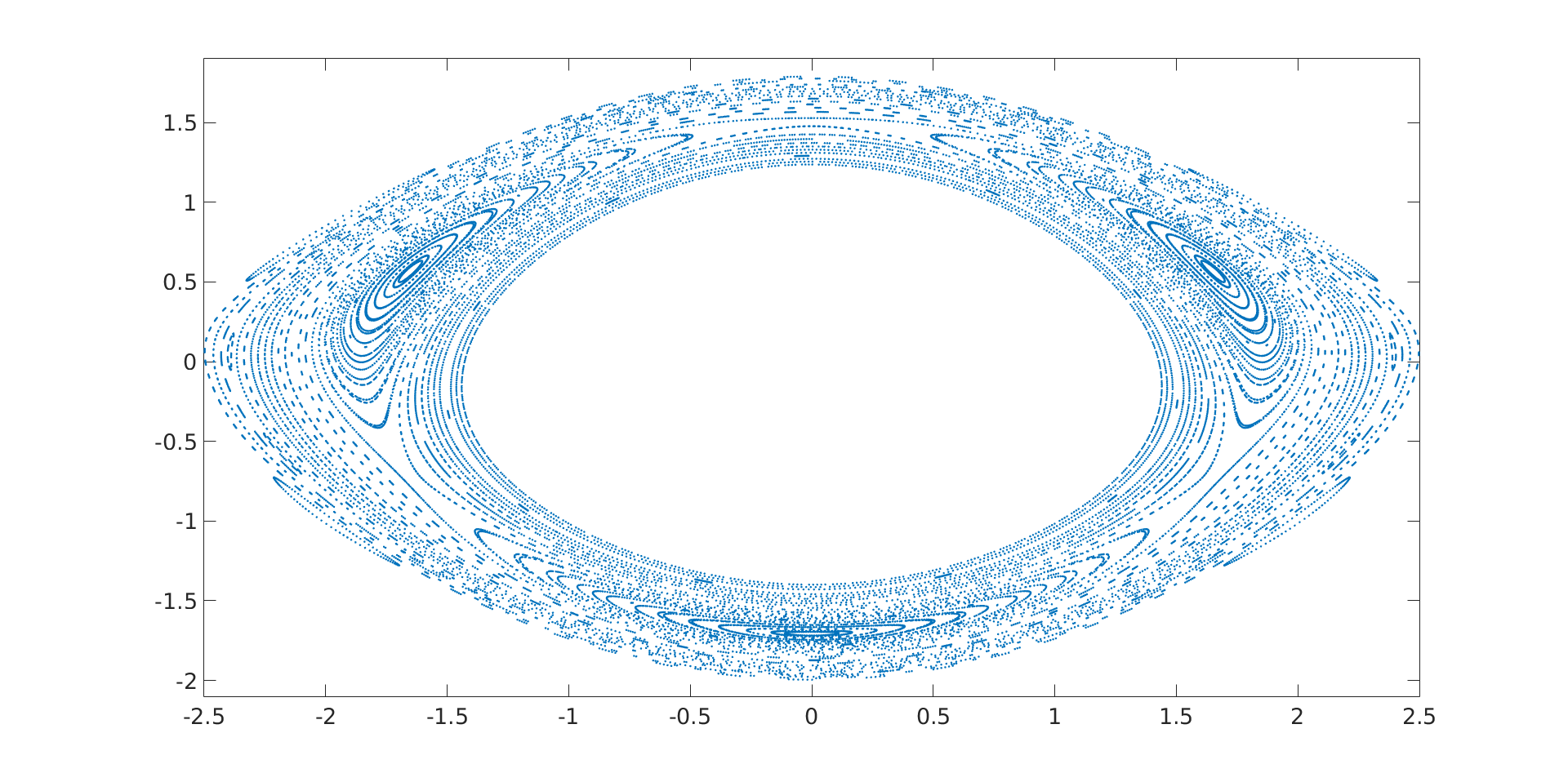
Figure 6: Dynamics of the stroboscopic map for $\varepsilon=0.2$ close to a $3$-periodic orbit for $t_{0}=0$. The figure has been obtained by iterating initial conditions along a line going through the elliptic periodic orbit surrounding the level of energy $H(0,1.6)$ and $T=T_{c}/3$.

In Figure 6 we show the dynamics of the stroboscopic map for $\varepsilon=0.2$ close to the level of energy $c=H(0,1.6)$ (chosen arbitrarily in Section 2.3) and $t_{0}=0$. When choosing $T=T_{c}/3$, one observes two $3$-periodic orbits. One periodic orbit is of the saddle type, and one iterate is close to the vertical axis. The other periodic orbit is of the elliptic type, as the three points of this periodic orbit are surrounded by (apparent) curves.

Exercise 6.

Use the code written in Exercise 4 to simulate the stroboscopic map of System (2) for $\varepsilon>0$ (small) in the following situations.

1. set $t_{0}$ and iterate initial conditions around a resonance of the unperturbed system. That is, choose $T=T_{c}/m$ for some $c\in(-1,1)$, iterate use some initial conditions along $(0,v_{0}-2\varepsilon)$ to $(0,v_{0}+2\varepsilon)$, with $c=\frac{v_{0}^{2}}{2}-1$. Alternatively, you can take initial conditions along a line (the diagonal for example): $(v_{1}-2\varepsilon,v_{1}-2\varepsilon)$ to $(v_{1}+2\varepsilon,v_{1}+2\varepsilon)$, with $H(v_{1},v_{1})=\frac{v_{1}^{2}}{2}-\cos{v_{1}}$. How many periodic orbits do you observe?

2. Repeat the same simulation choosing some $t_{0}=0$. What changes do you observe? What if you choose $t_{0}=T$?

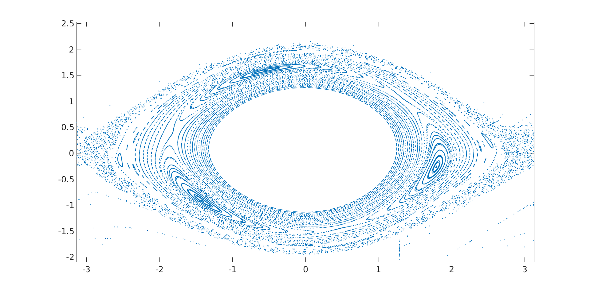
Figure 7: Dynamics of the stroboscopic map for $\varepsilon=0.2$ close to a $3$-periodic orbit for $t_{0}=1$. The figure has been obtained by iterating initial conditions along a line going through the elliptic periodic orbit surrounding the level of energy $H(0,1.6)$ and $T=T_{c}/3$.

Solution 5.

In Figure 6 we have what you should observe for $v_{0}=1.6$, $T=T_{c}/3$, $t_{0}=0$ and taking initial conditions along the line $y=0.5/1.6x$. In Figure 7 we have chosen $t_{0}=1$ and initial conditions along a straight line going through the elliptic periodic orbit. Note that the dynamics is the same as before but the portrait is twisted. As the system is $T$-periodic, one should observe the same for $t_{0}=T$ than for $t_{0}=0$.

Remark 2.

As for $\varepsilon>0$ System (2) is non-autonomous, the dynamics of the stroboscopic map depend on the election of $t_{0}$. However, the dynamics are qualitatively the same but twist when $t_{0}$ is varied. Compare Figures 6 and 7.

3 The Melnikov method for subharmonic periodic orbits

In Section 2.4 we have seen using numerical simulation that, when $T_{c}$ and $T$ are congruent, the corresponding periodic orbit may persist for $\varepsilon>0$. In this section we present a result (the Melnikov method) that provides sufficient conditions for the persistence of periodic orbits resonant with the period of the perturbation. Indeed, it does not only predict this persistence but also provides information regarding the location of these periodic orbits. As we will see in Section 4, this will become very useful when computing periodic orbits using Newton’s method.

3.1 Persistence of periodic orbits

The Melnikov method can be applied to a larger class of systems than the pendulum. More precisely, we consider a general planar field of the form

$$\dot{x}=f(x)+\varepsilon g(x,t)=\left(\begin{array}[]{c}f_{1}(x)\\ f_{2}(x)\end{array}\right)+\varepsilon\left(\begin{array}[]{c}g_{1}(x,t)\\ g_{2}(x,t)\end{array}\right),$$ (5)

where $x=(u,v)\in\mathbb{R}^{2}$, $\varepsilon\geq 0$ is a small parameter and $g(x,t)$ is $T$-periodic in $t$:

$$g(x,t+T)=g(x,t),\forall x\in\mathbb{R}^{2}.$$

For simplicity, let us assume that, for $\varepsilon=0$, the unperturbed system

$$\dot{x}=f(x)$$

is Hamiltonian. That is, there exists a function $H(u,v)$ such that

$$\dot{u} =\frac{\partial H(u,v)}{\partial v}$$

$$\dot{v} =-\frac{\partial H(u,v)}{\partial u}.$$

Moreover, let us assume that for $\varepsilon=0$, the system satisfies the following conditions:

1. There exists a compact region completely covered by a continuum of periodic orbits.

2. Let $T_{c}$ be the period of the periodic orbit located at the energy level $c$:

   $$\left\{(u,v)\in\mathbb{R}^{2},\,H(u,v)=c\right\}.$$

   Assume that $\frac{d}{dc}T_{c}\neq 0$.

Then we have the following result ([GH83, Mel63]):

Theorem 1.

Assume the above conditions are satisfied. Assume that the unperturbed system has a periodic orbit, $H(u,v)=c$, of period

$$T_{c}=\frac{m}{n}T,$$ (6)

where $T$ is the period of the periodic forcing. Let $x_{0}=(u_{0},v_{0})$ be an initial condition for such a periodic orbit (that is, $H(x_{0})=c$), and let

$$\varphi_{0}(t;x_{0})$$

be the unperturbed flow at such initial condition. Then let us define the so-called (subharmonic) Melnikov function

$$M(t_{0}) =\int_{0}^{mT}f(\varphi_{0}(t;x_{0}))\wedge g(\varphi_{0}(t;x_{0}),t+t_{0})dt$$ (7)

$$=\int_{0}^{mT}\Big{(}f_{1}(\varphi_{0}(t;x_{0}))\cdot g_{2}(\varphi_{0}(t;x_{0}),t+t_{0})$$

$$\quad-f_{2}(\varphi_{0}(t;x_{0}))\cdot g_{1}(\varphi_{0}(t;x_{0}),t+t_{0})\Big{)}dt.$$

Then, if there exists $\bar{t}_{0}$ such that

1. $M(\bar{t}_{0})=0$

2. $M^{\prime}(\bar{t}_{0})\neq 0$,

then, for $\varepsilon>0$ small enough, the perturbed system possesses a periodic orbit of period $mT$ with initial condition $x_{\varepsilon}=x_{0}+O(\varepsilon)$ at $t=\bar{t}_{0}:$

$$\varphi_{\varepsilon}(\bar{t}_{0}+mT;\bar{t}_{0},x_{\varepsilon})=x_{\varepsilon}.$$

Remark 3.

The Melnikov function does not require to compute the perturbed flow. One just needs to evaluated the cross product of the unperturbed field and the perturbation along a solution of the unperturbed system, $\varphi_{0}(t;x_{0})$.

Remark 4.

Given $n$, $m$ and $T_{c}=\frac{mT}{n}$, the Melnikov function depends on the election of $x_{0}$ at the periodic orbit $H(u,v)=c$.

Remark 5.

The Melnikov function is $mT$-periodic.

Exercise 7.

Compute the analytical expression of the integrand of the Melnikov function for system (3) (you don’t have to do the integral!).

Exercise 8.

Write a little program in Matlab to numerically compute the Melnikov integral obtained in Exercise 7.

1. Try different $n$’s and $m$’s. Do you always observe zeros of the Melnikov function?

2. Try a different perturbation with higher harmonics, for example $g(t)=\sin(\omega t)+4\cos(2\omega t)$. What do you observe?

Solution 6.

The function melnikov.m performs the Melnikov integral. However, the initial condition for the unperturbed periodic orbit has to be properly set. One option is to proceed as in previous exercises: fix a periodic orbit of the unperturbed system given by some energy level $H(u,v)=c\in(-1,1)$ by fixing its initial condition at the vertical axis: $H(0,v_{0})=\frac{v_{0}^{2}}{2}-1=c$. Then, using the function period.m from Exercise 3 we compute $T_{c}$. Given $n$ and $m$, the period $T$ of the forcing becomes $T=nT_{c}/m$.
However, in real applications, we may have a given fixed $T$. In this case, we need to find the level of energy $c$ corresponding to $T_{c}=mT/n$. This could be done by combining the function period.m from Exercise 3 and the Matlab routine fzero to obtain the initial condition of an $nT/m$ periodic orbit of the unperturbed system.
Anyhow, once we have $n$, $m$, $T$ and $x_{0}$ we compute the Melnikov integral of Theorem 1.

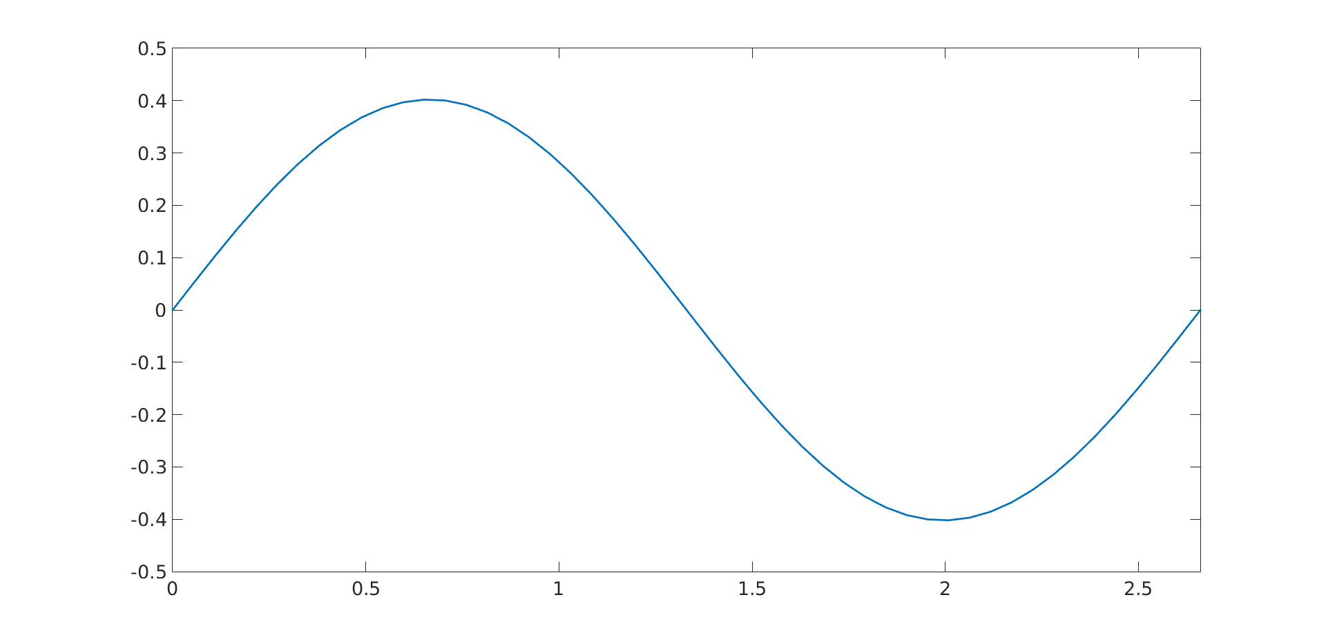
(a)

(b)

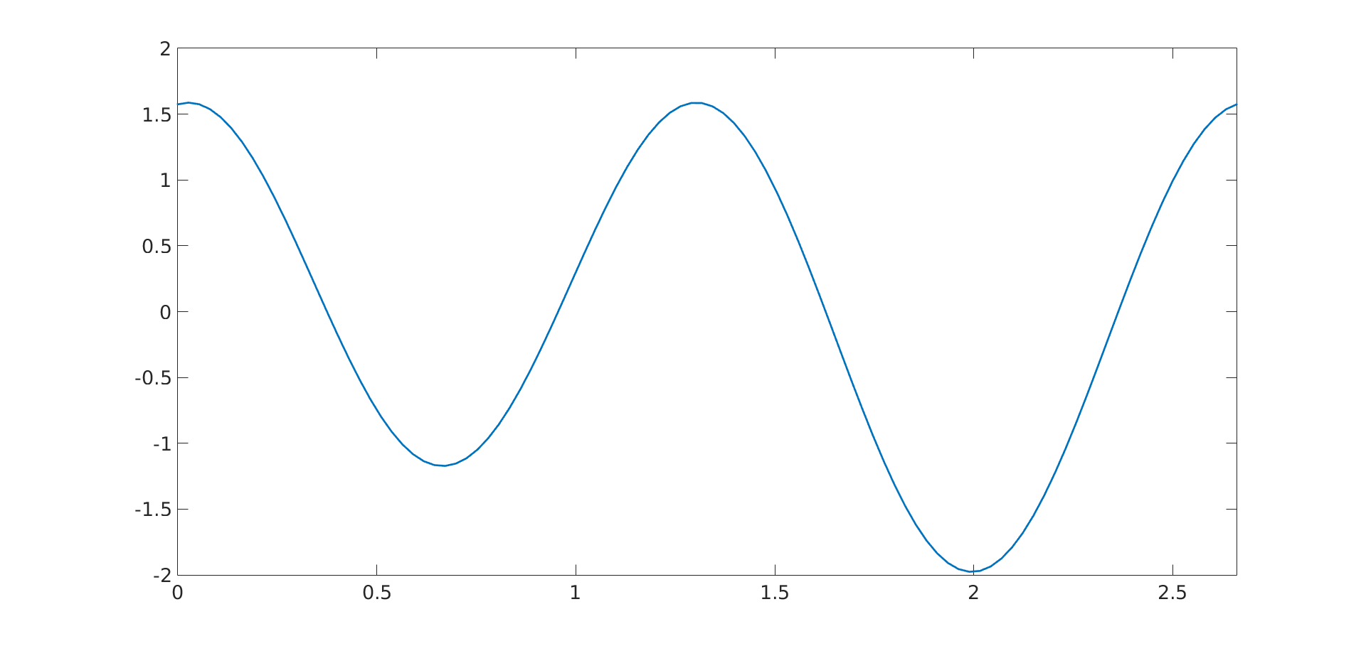
(c)

Figure 8: Melnikov function for $g(x,t)=\sin(\omega t)$ (a) and $g(x,t)=\sin(\omega t)+20\cos(2\omega t)$ (b) and $g(x,t)=\sin(\omega t)+10^{7}\cos(2\omega t)$ (c).

In Figure 8 we show the Melnikov function for three different perturbations for $m=3$ and $n=1$. Note that Figures 8(a) and 8(b) are almost the same even if the second one contains a higher harmonic. However, as shown in Figure 8(c), if the weight of the second harmonic is drastically increased, then new zeros appear leading to more periodic orbits. Note however that, as this weight is so high, the value of $\varepsilon$ for which one can observe the new periodic orbits may be extremely small.

When considering the subharmonic case $n=2$ and $m=3$ corresponding to rotation number $2/3$, it turns out that the Melnikov function is identically zero for $g(x,t)=\sin(\omega t)$. Therefore, one cannot prove nor discard the existence of $3$-periodic orbit with rotation number $2/3$ for such a perturbation and a second order analysis is required. However, as shown in Figure 9 when simulating the stroboscopic map, there is no evidence of existence of such a periodic orbit.

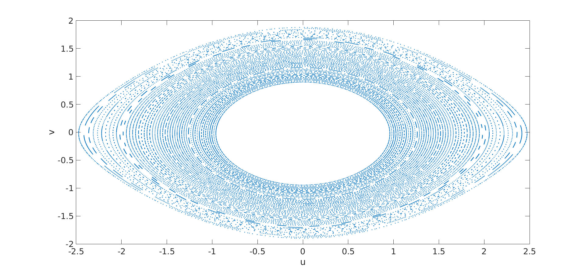
Figure 9: Dynamics of the stroboscopic map for $g(x,t)=\sin(\omega t)$ and $\varepsilon=0.01$ around the unpertubed periodic orbit with rotation number $2/3$. Such periodic orbit does not seem to persist for $\varepsilon>0$.

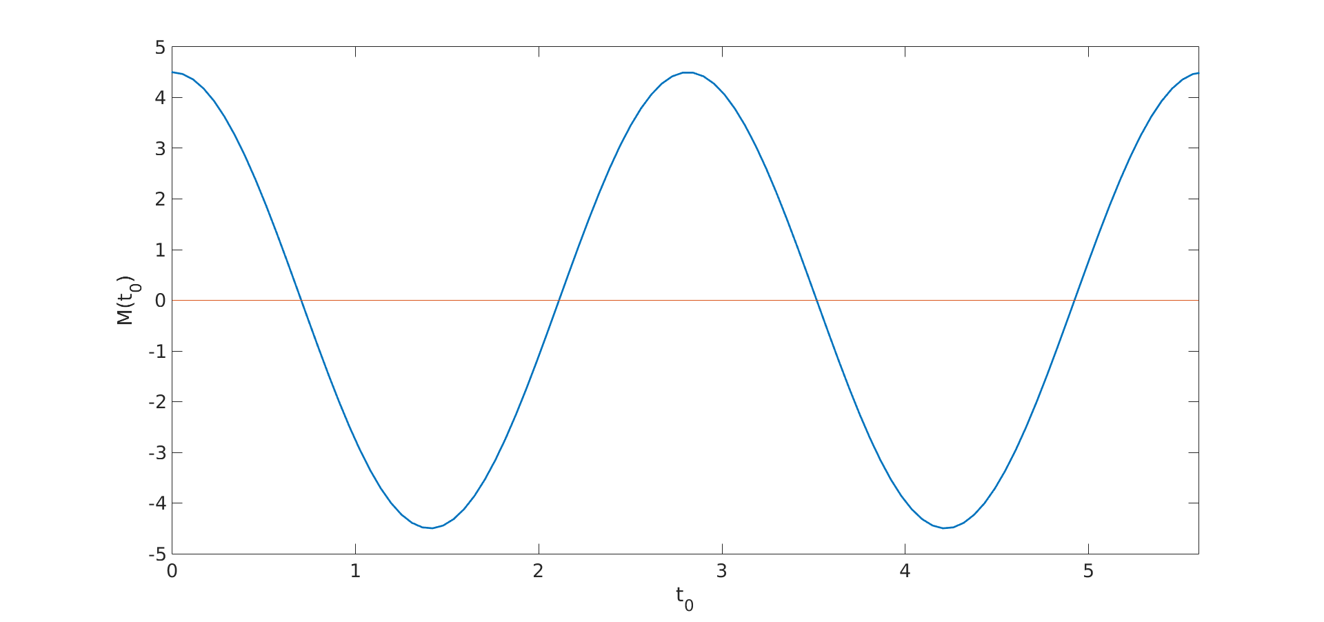
Figure 10: Melnikov function for $g(x,t)=\sin(\omega t)+4\cos(2\omega t)$ using $x_{0}=(0,1.7)$, $\omega=\frac{2\pi}{T}$, $T=\frac{2T_{c}}{3}$ and $c=H(0,1.7)$.

However, as shown in Figure 10, when using a pertubation with higher harmonics such as $g(x,t)=\sin(\omega)+4\cos(2\omega t)$, the Melnikov function possesses simple zeros.

3.2 Interpretation

As we have seen in Section 2.3, when $\varepsilon=0$, when $T_{c}=mT/n$, all points satisfying $H(u,v)=c$ are $m$-periodic points of the stroboscopic map. However, for $\varepsilon>0$, only some of these points may persist as $m$-periodic points of the perturbed stroboscopic map. Therefore the following question arises: given an $m$-periodic point $x_{0}$ satisfying $H(x_{0})=c$ does this point persist after the perturbation? In other words, does it exist some point $x_{\varepsilon}$ $\varepsilon$-close to $x_{0}$ such that

$$s^{m}(x_{\varepsilon})=x_{\varepsilon}?$$

Taking into account Theorem 1, the answer is that this depends on $t_{0}$. That is, once we have chosen $x_{0}$, the (simple) zeros of the Melnikov function provides us the proper values of $t_{0}$ such that $x_{\varepsilon}$ exists and is $\varepsilon$-close to $x_{0}$.
Recalling exercise 6, when $\varepsilon>0$ (small), the stroboscopic may exhibit isolated periodic points. These points are $\varepsilon$-close to the curve given by $H(u,v)=c$ (periodic orbit of the unperturbed system); however, these points twist when $t_{0}$ is varied. The zeros of the Melnikov function tell us how much do we have to twist in order to have one of these points $\varepsilon$-close to the chosen $x_{0}$.

4 Computation of periodic orbits using the stroboscopic map

We now want to numerically compute the initial condition ($x_{\varepsilon}$) for a periodic orbit given by Theorem 1. Here we describe a Newton method to do that in a general setting: $n$-dimensional not necessary Hamiltonian system.

Assume we want to compute a periodic orbit of an $n$-dimensional non-autonomous periodic system of the form

$$\dot{x}=f(x,t),$$ (8)

where $f(x,t)$ is a $T$-periodic field in $t$: $f(x,t+T)=f(x,t)$, for any $x\in\mathbb{R}^{n}$.
Due to the periodicity, instead of using Poincaré maps in the state space it will be much more convenient to use the so-called stroboscopic map, which is indeed a Poincaré map in the extended state space (adding time as a variable and using a section in time). This map is given by flowing system (8) for a time $T$ with initial condition $(x_{0},t_{0})$:

$$s(x_{0})=\varphi(t_{0}+T;x_{0},t_{0}).$$

Provided that system (8) is $T$-periodic in $t$, $s(x)$ becomes a map from the time section $t=t_{0}$ to itself:

$$\begin{array}[]{cccc}s:&\Sigma_{t_{0}}&\longrightarrow&\Sigma_{t_{0}}\\ &x&\longmapsto&\varphi(t_{0}+T;x,t_{0}),\end{array}$$

where

$$\Sigma_{t_{0}}=\left\{(x,t)\in\mathbb{R}^{2}\times\mathbb{T}_{T}\right\},\,\mathbb{T}_{T}:=\mathbb{R}/T\mathbb{Z}.$$

Imagine that we want to compute the initial condition, $x^{p}$ for a periodic orbit of system (8) at the section $\Sigma_{t_{0}}$. Recalling its periodicity, the period of such a periodic orbit must be a multiple of $T$, say $mT$. In other words, we must look for periodic points of the map $s$, that is, points $x^{p}$ such that

$$s^{m}(x^{p})=x^{p}.$$

One of the most extended methods for numerically computing such points is the Newton method, assuming that one has some idea about where such a points lies, as we need a first approximation for the Newton method to converge where we want.

4.1 Newton method for fixed points

Let us assume that we are looking for a $T$-periodic orbit; that is, $m=1$ and we want to find a fixed point of the map $s$. Then, we want to solve the equation

$$F(x):=s(x)-x=0.$$

The Newton method consists of considering the linear approximation of the function $F$ around some point $(x_{0},F(x_{0}))$ (which is a first approximation of the solution we are looking for) and solve the linear system instead. This provides a new point, $(x_{1},F(x_{1}))$ which, hopefully, is a more accurate solution than the initial one.
The linear approximation of equation $F(x)=0$ around $(x_{0},F(x_{0}))$ becomes

$$F(x_{0})+DF(x_{0})(x-x_{0})=0,$$ (9)

where

$$DF(x_{0})=Ds(x_{0})-I.$$

In Section 4.3 we will see how to compute the differential $D_{x}s(x)$.
If we solve Equation (9) for $x$ we get

$$x=x_{0}-\big{(}DF(x_{0})\big{)}^{-1}F(x_{0}).$$

This leads to an iterative process

$$x_{i+1}=x_{i}-(DF(x_{i}))^{-1}F(x_{i}),$$ (10)

which converges quadratically to $x^{p}$ provided that $x_{0}$ is a good enough approximation.
Alternatively, some programing environments (like Matlab) offer routines to solve linear equations which might be more efficient than computing the inverse $(DF(x_{0}))^{-1}$. In this case, we can consider the linear equation

$$DF(x_{i})x_{i+1}=DF(x_{i})x_{i}-F(x_{i}),$$ (11)

which we want to solve for $x_{i+1}$.

Remark 6.

Note that the Newton method requires the matrix $DF(x_{i})$ to be invertible. This implies two things:

• $DF$ must be invertible at the starting point

• $DF$ must be invertible at the fixed point! This implies that the Newton method will have troubles if the fixed point we are looking for has a eigenvalues real eigenvalue equal to $1$. Note that, as $Ds$ and $Id$ commute, the eigenvalues of $DF$ are the one of $Ds$ minus one. In two dimensions, this is degenerate and pathological, but possible. In dimension one this occurs frequently.

4.2 Newton method for periodic orbits

Similarly we can apply the Newton method to solve the equation

$$F(x)=s^{m}(x)-x$$

to get the same expression as in Eq. (10). However, in this case the computation of $DF$ becomes now a bit more tricky. Using that $s^{i}(x)=s(s^{i-1}(x))$, we apply the chain rule to get

$$DF(x_{i})=\prod_{j=i}^{j=1}Ds(s^{j-1}(s)),$$

se we need to evaluate the differential $Ds(x)$ at the points $s^{j}(x)$ for $j=1..i$.

Although there is nothing wrong with this approach from the theoretical point of view, in next section we will see a numerical method to compute $Ds(x)$ which makes the computation of $Ds^{m}(x)$ straightforward, without needing to multiply matrices (see Remark 9 below).

4.3 Computation of the differential of the stroboscopic map: the variational equations

Now the question arises, how do we compute $Ds$? Note that the flow $\varphi(t;x_{0},t_{0})$ is straightforward to differentiate with respect to $t$, as one recovers the field $f$, but we need to differentiate it with respect to the initial condition $x_{0}$! But we can do the following. Applying the fundamental theorem of calculus and the definition of the flow, we can write

$$s(x_{0}) =\varphi(t_{0}+T;x_{0},t_{0})=x_{0}+\int_{t_{0}}^{t_{0}+T}\frac{d}{dt}\varphi(t;x_{0},t_{0})dt$$

$$=x_{0}+\int_{t_{0}}^{t_{0}+T}f(\varphi(t;x_{0},t_{0}),t)dt.$$

If we now differentiate with respect to $x_{0}$, we get

$$Ds(x_{0})=I_{n}+\int_{t_{0}}^{t_{0}+T}Df\left(\varphi(t;x_{0},t_{0}),t\right)\cdot D_{x_{0}}\varphi(t;x_{0},t_{0})dt,$$ (12)

where $I_{n}$ is the $n\times n$ identity matrix and we write $D_{x_{0}}$ to emphasize that we differentiate with respect to $x_{0}$, while $Df$ is the Jacobian of $f$. Again, by applying the fundamental theorem of calculus backwards, we realize that Equation (12) is the solution of the differential equation

$$\frac{d}{dt}D_{x_{0}}\varphi(t;x_{0},t_{0})=Df(\varphi(t;x_{0},t_{0}))\cdot D_{x_{0}}\varphi(t;x_{0},t_{0}),$$ (13)

at $t_{0}+T$. Equation (13) is called the (first) variational equation.
There is however a more straightforward argument to obtain the variational equations. If we just differentiate

$$\frac{d}{dt}D_{x_{0}}\varphi(t;x_{0},t_{0}),$$

by commuting $Dx$ and $d/dt$ (which is possible of $\varphi$ is at least $C^{2}$ with respect to $t$ and $x_{0}$), we obtain

$$\frac{d}{dt}D_{x_{0}}\varphi(t;x_{0},t_{0})=D_{x_{0}}\frac{d}{dt}\varphi(t;x_{0},t_{0})=D_{x_{0}}f\left(\varphi(t;x_{0},t_{0})\right).$$

Applying the chain rule we obtain

$$\frac{d}{dt}D_{x_{0}}\varphi(t;x_{0},t_{0})=Df\left(\varphi(t;x_{0},t_{0})\right)\cdot D_{x_{0}}\varphi(t;x_{0},t_{0})$$

Some remarks:

Remark 7.

If $f(x,t)$ is a field in $\mathbb{R}^{n}$, then this equation becomes and $n\times n$-dimensional differential equation.

Remark 8.

Equation (13) is evaluated along the flow $\varphi(t;x_{0},t_{0})$, which is unknown. Hence, this equation needs to be solved together with the equation $\dot{x}=f(x,t)$, leading to a total system of dimension $n+n\times n$ with initial condition $(x,I_{n})$.

Remark 9.

If we want to compute $Ds^{m}(x)$, we just need to integrate the variational equations from $t_{0}$ to $t_{0}+mT$!

Exercise 9.

Obtain the variational equations for the perturbed pendulum.

4.4 Combining Newton and Melnikov’s method

Let us now consider a system as in Equation (5) satisfying conditions  M.1-M.2. As seen in Sections 2, some of the periodic orbits that exist for $\varepsilon=0$ (given as curves $H(u,v)=c$) may persist after the perturbation. In particular, one needs congruency between the period of the perturbation and the unperturbed periodic orbit: $nT_{c}=mT$ for some $m$ and $n$ co-prime integers.
When computing periodic points for $\varepsilon>0$ using the Newton method described in Section 4.2, it becomes natural to use some $x_{0}$ satisfying $H(x_{0})=c$ as a seed for the Newton method, as these periodic points are $\varepsilon$-close to the curve given by $H(u,v)=c$. However, unlike in the unperturbed case, periodic points of the perturbed stroboscopic map become isolated and hence not any $x_{0}$ with $H(x_{0})=c$ will make the Newton method converge to the desired point. However, recalling that the system is non-autonomous, their location depends on the election of $t_{0}$. This is where the Melnikov method becomes constructive by providing a proper seed. More precisely, the Melnikov method purposes to choose $x_{0}$ arbitrarily at the curve $H(u,v)=c$ and then use a proper value of $t_{0}$ ($\bar{t}_{0}$ a zero of $M(t_{0})$) such that the desired periodic point, $x_{\varepsilon}$, is $\varepsilon$-close to $x_{0}$. Hence, if $\varepsilon>0$ is small enough and $t_{0}=\bar{t}_{0}$ is chosen to be a simple root of the Melnikov function, the Newton method will quadratically converge to $x_{\varepsilon}$ when using $x_{0}$ as initial guess.

Exercise 10.

Write a program in Matlab in order to compute $nT/m$-periodic orbits for $\varepsilon>0$.

1. Obtain the variational equations and write them in the file pertpend_vari.m.

2. Implement the Newton method to obtain a fixed point of the stroboscopoic map. You will need to tune $\omega$ to guarantee that it exists. In the file Newton.m you have some lines that you can use. Note that the initial seed will be taken from a zero of the Melnikov function, which may have several. First use an initial seed obtained manually to make sure that your program works.

3. Perform a veeeery little modification in your program to compute $nT$-periodic orbits instead of a $T$-periodic orbit. Compute the eigenvalues of $Ds$ at these periodic orbits. What is their type?

Solution 7.

The variational equations are easy to obtain.
The routine Newton.m contains one step of the Newton method. By repeating this step until the norm of $F$ is small enough, we we perform a Newton method for a fixed point. Just by replacing $T$ by $mT$, the program will compute an $m$-periodic orbit instead of a fixed point.
Now we use the program. We choose to compute a $3$-periodic orbit with rotation number $1/3$. Hence, we use as seed a point satisfying $H(x_{0})=c$, form some $c$, and use $T=\frac{T_{c}}{3}$ and $\omega=\frac{2\pi}{T}$. We choose for example value we used in previous exercises: $x_{0}=(0,1.6)$ and $c$ becomes $c=\frac{1.6^{2}}{2}-1$. The Melnikov function for $g(x,t)=\sin(\omega t)$ is shown in Figure 8(a), and possess two simple zeros: $\bar{t}_{0}=0$ and $\bar{t}_{0}=T/2\simeq 1.4$. Using $x_{0}=(0,1.6)$ and $t_{0}=0$ as seed for the Newton method, we show in Figure 11 how the method diverges for $\varepsilon=0.05$. By reducing $\varepsilon$ to $\varepsilon=0.4$ the Newton method converges to another periodic orbit. By further decreasing $\varepsilon$ to $\varepsilon=0.01$, the Newton method finally converges to the desired periodic orbit (a saddle). In Figure 12 we show how the method converges in 6 iterations reaching an accuracy of $10^{-8}$. By using the obtained result as seed for a next Newton method we can follow up this periodic orbit by increasing $\varepsilon$. In Figure 13 we show what we obtain for $\varepsilon=0.17$.

We now focus on the other periodic orbit given by the zero of the Melnikov function around $\bar{t}_{0}=T/2\simeq 1.33$. Proceeding similarly, by continuation of the Newton method, we can follow this periodic orbit (of the elliptic type) up values higher than $\varepsilon=5$. In Figure 14 we show the iterates of the stroboscopic map of this periodic orbit for $\varepsilon=2.9$ and the dynamics surrounding it. As we can see there, very little of the rest of the dynamics persist for such large value of $\varepsilon$. However, when zooming in (see Figure 15), we observe secondary tori and secondary periodic orbits around the elliptic periodic orbit. In Figure 16 we show the time-continuous evolution of $u$ and $v$ along this periodic orbit. As can see, the periodic orbit takes $3$ times $T$ to perform one loop around the origin, hence reflecting the rotation number $1/3$.

We finally discuss the case of rotation number $2/3$. As explained in Exercise 8, we need to include higher harmonics in order to guarantee the existence of such periodic orbits; otherwise, the Melnikov function becomes identically zero. Proceeding as before, using $g(x,t)=\sin(\omega t)+3\cos(2\omega t)$, $\omega=\frac{2\pi}{T}$, $T=\frac{2T_{c}}{3}$, $c=H(0,1.7)$, we use $\bar{t}_{0}=0.7035$ (first zero of Figure 10) and $x_{0}=(0,1.7)$ as seed for the Newton method. Starting with a small $\varepsilon$ and performing continuation, we obtain the periodic orbit with rotation number $2/3$ shown in Figure 17 for $\varepsilon=0.5$. As can see there, the periodic orbit performs $2$ loops when closing at $t=\bar{t}_{0}+3T$.

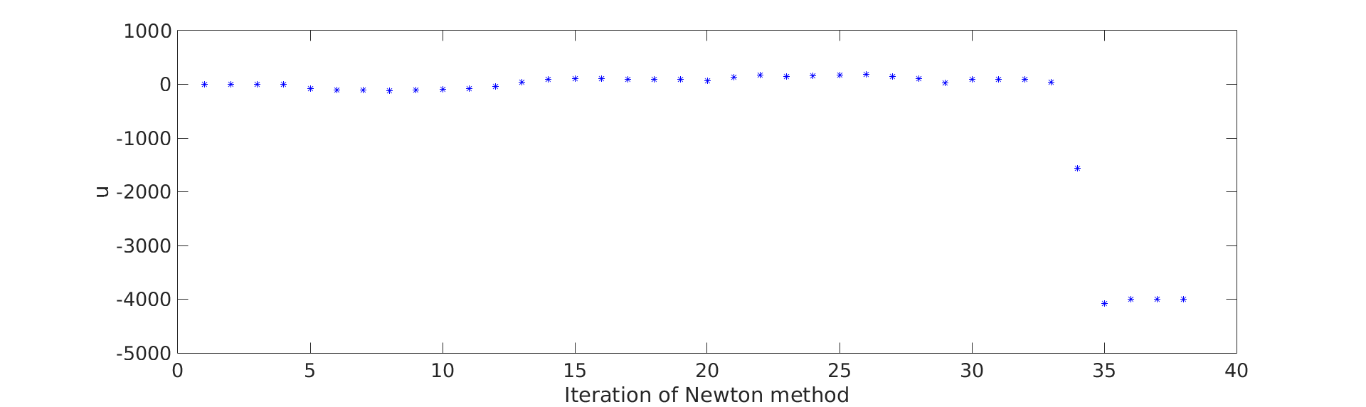
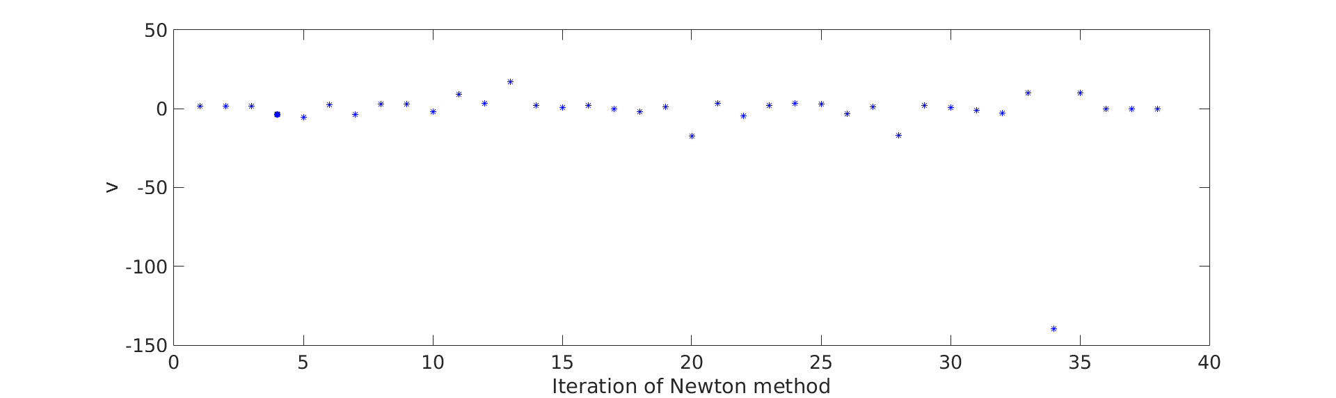
Figure 11: Diverging Newton method for $\varepsilon=0.05$, initial seed $x_{0}=(0,1.6)$, $t_{0}=0$, $T=\frac{T_{c}}{3}$ and $c=H(0,1.6)$.

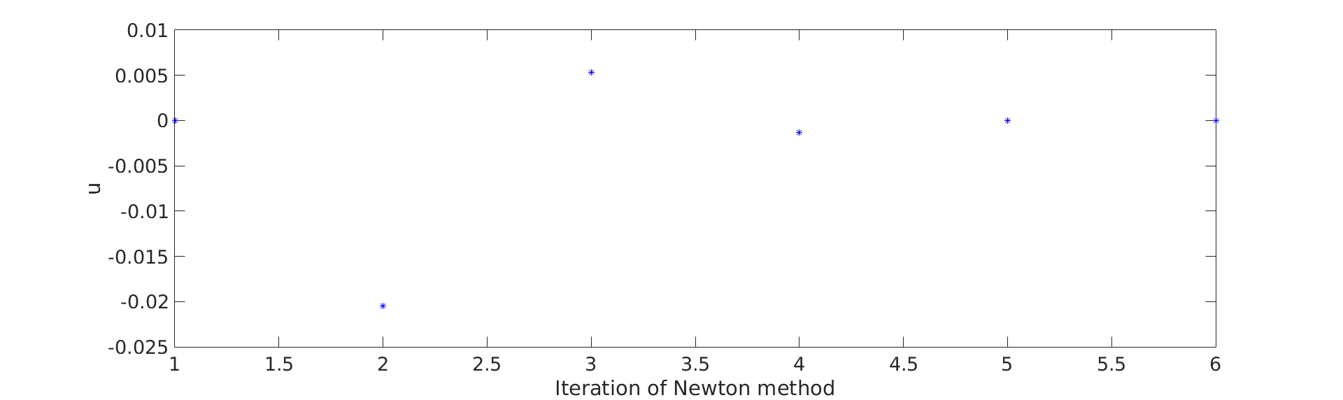
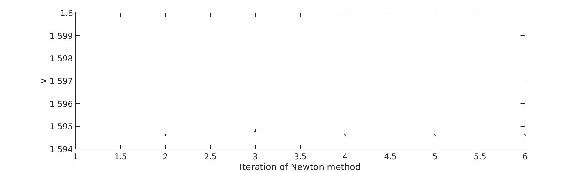
Figure 12: Iterates of the Newton method converging to a saddle periodic orbit with $\varepsilon=0.01$ and the rest values as in Figure 11.

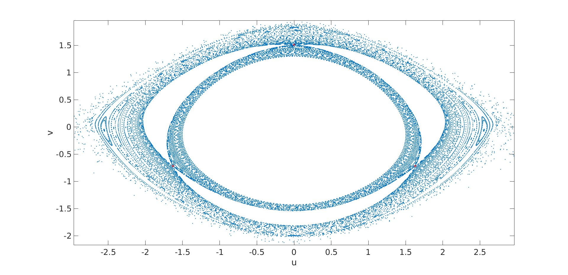
Figure 13: Saddle periodic orbit with rotation number $1/3$ for $\varepsilon=0.17$. The red point close the vertical axis is obtained by continuation of the Newton method. The other two points ar its iterates.

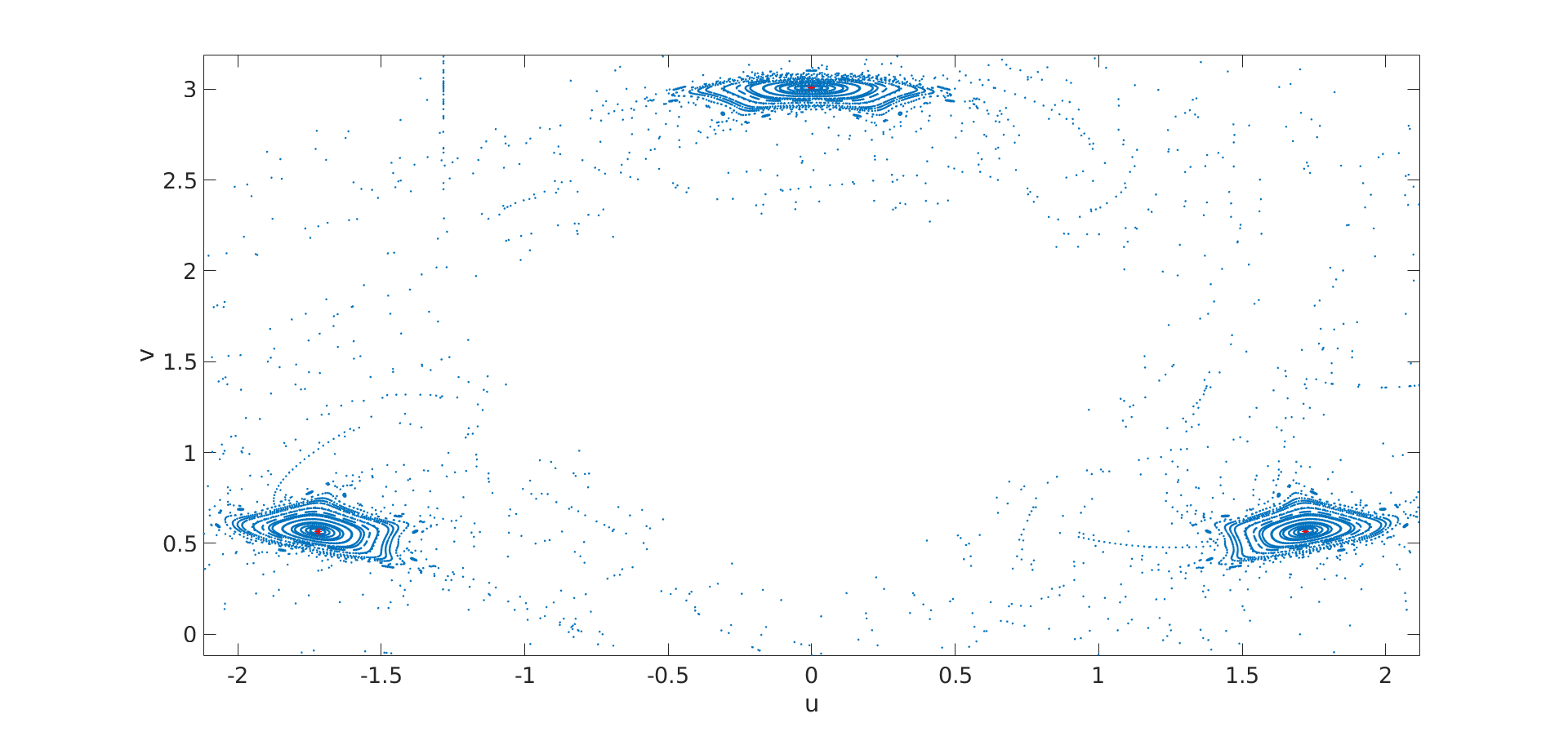
Figure 14: Elliptic $3$-periodic orbit for $\varepsilon=2.9$ and $t_{0}=\bar{t}_{0}=T/2\simeq 1.33$.

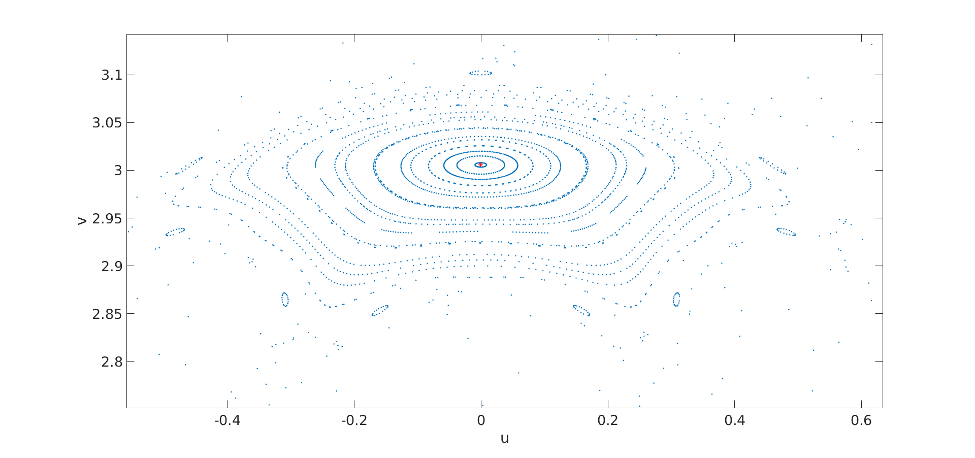
Figure 15: Zoom of Figure 14. In blue the dynamics of the stroboscopic map, in red the iterates of the periodic orbit found using the Newton method.

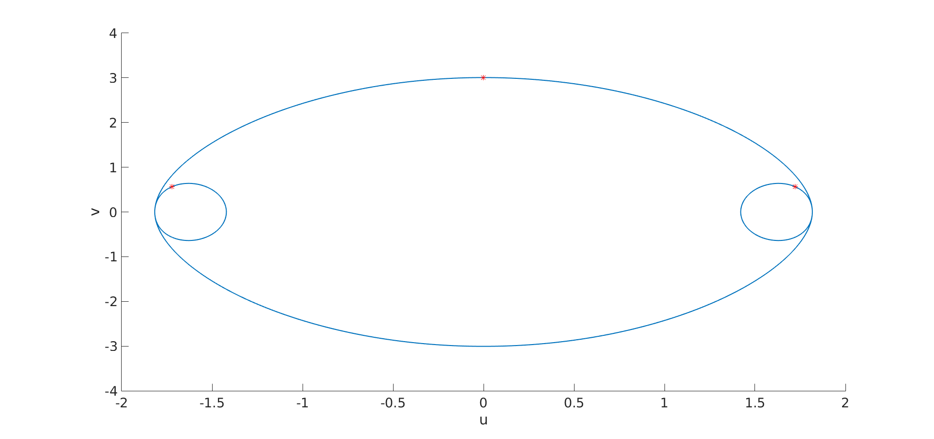
Figure 16: Time-continuous trajectory for $t\in[T/2,T/2+3T]$ corresponding to the $3$-periodic orbit shown in Figure 14 (blue curve). Red points are the iterates of the stroboscopic map.

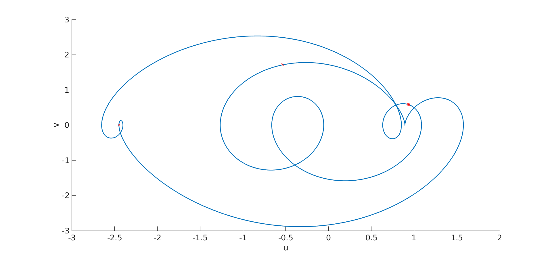
Figure 17: Periodic orbit with rotation number $2/3$ for $g(x,t)=\sin(\omega t)+4\cos(2\omega t)$ and $\varepsilon=0.5$.

5 Computation of periodic orbits using a Poincaré map

As noted in Remark 6, the Newton method to find fixed points (or periodic orbits) of the stroboscopic map may fail if that one has a real eigenvalue equal to $1$. Alternatively, we can use a Poincaré map using a section in the state space. This method is more robust in that sense, but, as we will show below, the computation of the differential becomes slightly more tricky.

Let us consider the Poincaré map

$$\begin{array}[]{cccc}P_{\varepsilon}(v,t):&\left\{u=0\right\}\times\mathbb{R}&\longrightarrow&\left\{u=0\right\}\times\mathbb{R}\\ &(0,v_{0},t_{0})&\longmapsto&(0,\varphi_{1}(t^{*};0,v_{0},t_{0}),t^{*}),\end{array}$$ (14)

where

$$\varphi_{\varepsilon}(t;x_{0},t_{0})=\left(\begin{array}[]{c}\varphi_{1}(t;x_{0},t_{0})\\ \varphi_{2}(t;x_{0},t_{0})\end{array}\right)$$ (15)

is the solution of the perturbed system (1) with initial condition $x_{0}$ at $t=t_{0}$ and $t^{*}$ is such that

$$\varphi_{1}(t^{*};0,v_{0},t_{0})=0$$ (16)

for the second time, as we consider a return map in the direction that the section is left.
Recall that system (1) is non-autonomous. Hence, the initial time $t_{0}$ matters and we have to carry it on. From now on, we will abuse notation in Equation (14) and omit writing the first coordinate $u$, as it takes the $0$.

Taking into account the periodicity of the non-autonomous system (1), an initial condition at $(0,v_{0})\in\left\{u=0\right\}$ for $t=t_{0}$ of a periodic orbit of the full system will need to satisfy

$$P^{n}(v_{0},t_{0})=\left(\begin{array}[]{c}v_{0}\\ t_{0}+mT\end{array}\right)$$ (17)

for some $n,m>0$. Indeed, the integers $n$ and $m$ are the same as in previous sections, made explicit through the congruency equation (6). Here one clearly see that the role of $n$ is to count the “loops” that a periodic orbit of period $mT$ makes around the origin.

Applying the Newton method to the equation

$$F(v_{0},t_{0})=P^{n}(v_{0},t_{0})-\left(\begin{array}[]{c}v_{0}\\ t_{0}+mT\end{array}\right)=\left(\begin{array}[]{c}0\\ 0\end{array}\right),$$ (18)

and arguing as in Section 4 we get the iterative process

$$(v_{i+1},t_{i+1})=(v_{i},t_{i})-(DF(v_{i},t_{i}))^{-1}F(v_{i},t_{i}),$$ (19)

where now

$$DF(v_{i},t_{i})=DP^{n}(v_{i},t_{i})-\left(\begin{array}[]{cc}1&0\\ 0&1\end{array}\right).$$

We now wonder, how do we compute $DP^{n}$? Let us see it for $n=1$ first.

Recalling that $\varphi_{\varepsilon}=\left(\varphi_{1},\varphi_{2}\right)$, we get

$$DP(v_{0},t_{0})=\left(\begin{array}[]{cc}D_{v_{0}}\varphi_{2}(t^{*};0,v_{0},t_{0})&D_{t_{0}}\varphi_{2}(t^{*};0,v_{0},t_{0})\\ \frac{\partial}{\partial v_{0}}t^{*}&\frac{\partial}{\partial t_{0}}t^{*}\\ \end{array}\right).$$

Note that, in the first row, we have written the total derivatives $D_{v_{0}}$ and $D_{t_{0}}$ instead of partial ones, $\partial/\partial v_{0}$ and $\partial/\partial_{t_{0}}$, because $t^{*}$ actually depends on $v_{0}$ and $t_{0}$ through Equation (16). Let us compute such total derivatives.
For the first one we get

$$D_{v_{0}}\varphi_{2}(t^{*};0,v_{0},t_{0})=\frac{\partial}{\partial v_{0}}\varphi_{2}(t^{*};0,v_{0},t_{0})+\varphi_{2}^{\prime}(t^{*};0,v_{0},t_{0})\frac{\partial t^{*}}{\partial v_{0}}.$$

Let us now see how to compute all the terms appearing in this equation.
On one hand,

$$\varphi_{2}^{\prime}(t^{*};0,v_{0},t_{0})=f_{2}(\varphi_{\varepsilon}(t^{*};0,v_{0},t_{0}))+\varepsilon g_{2}\left(\varphi_{\varepsilon}\left(t^{*};0,v_{0},t_{0}),t^{*}\right)\right),$$

where $f_{2}+\varepsilon g_{2}$ is the second coordinate of the field evaluated at the image of the Poincaré map.
On the other one, $\frac{\partial\varphi_{2}(t^{*};0,v_{0},t_{0})}{\partial v_{0}}$ is given by integrating the variational equations from $t_{0}$ to $t^{*}$, as we are differentiating with respect an initial condition.
What about $\frac{\partial t^{*}}{\partial v_{0}}$? Recall that, for given $v_{0}$ and $t_{0}$, $t^{*}$ (which we somehow know how to compute) solves Equation (16). Therefore, assuming that

$$\varphi_{1}^{\prime}(t^{*};0,v_{0},t_{0})\neq 0,$$ (20)

we can use the Implicit Function Theorem to get

$$\frac{\partial t^{*}}{\partial t_{0}} =-\frac{\frac{\partial}{\partial t_{0}}\varphi_{1}(t^{*};0,v_{0},t_{0})}{\varphi_{1}^{\prime}(t^{*};0,v_{0},t_{0})}$$

$$=-\frac{\frac{\partial}{\partial t_{0}}\varphi_{1}(t^{*};0,v_{0},t_{0})}{f_{1}(\varphi_{\varepsilon}(t^{*};0,v_{0},t_{0}))+\varepsilon g_{1}(\varphi_{\varepsilon}(t^{*};0,v_{0},t_{0}),t^{*})}.$$ (21)

Note that, condition (20) is satisfied, as the flow is transversal to the section $\left\{u=0\right\}$. If it were tangent, then we would have a problem, of course!
The denominator of the last equation is just the first coordinate of the perturbed field evaluated at the image of the Poincaré map.
Regarding $\frac{\partial}{\partial t_{0}}\varphi_{1}(t^{*};0,v_{0},t_{0})$, note that it is a derivative with respect to the initial time, $t_{0}$. Adding time as a variable, this can be computed integrating the variational equations of the system

$$\dot{u} =v$$ (22)

$$\dot{v} =-\sin(u)+\varepsilon\sin(\omega s)$$

$$\dot{s} =1,$$

where now $s$ plays the role of time and $t_{0}$ becomes $s_{0}$.

Proceeding similarly, the elements of the second row of $DP$ become

$$\frac{\partial t^{*}}{v_{0}}=-\frac{\frac{\partial}{\partial v_{0}}\varphi_{1}(t^{*};0,v_{0},t_{0})}{f_{1}(\varphi_{\varepsilon}(t^{*};0,v_{0},t_{0}))+\varepsilon g_{1}\left(\varphi_{\varepsilon}(t^{*};0,v_{0},t_{0})\right)},$$

and $\frac{\partial t^{*}}{\partial t_{0}}$ is already given in Equation (21)

The differential $DP^{n}(v_{0},t_{0})$ can be computed proceeding similarly as in Section 4.2, mutliplying $DP$ evaluated at the iterates $P^{n}(v_{0},t_{0})$ or integrating the previous variational equations until the $2n$-th impact with the section $\left\{u=0\right\}$ occurs.

Exercise 11.

Compute analytically the variational equations of system (22).

Exercise 12.

Write a program in Matlab to compute initial conditions for periodic orbits by performing a Newton method to Equation (18). For that you will need to use all the artillery you developed in the previous exercises.

References

- [GH83] J. Guckenheimer and P. J. Holmes. Nonlinear Oscillations, Dynamical Systems and Bifurcations of Vector Fields. Appl. Math. Sci. Springer, 4th edition, 1983.
- [Mel63] V.K. Melnikov. On the stability of the center for time–periodic perturbations. Trans. Moscow Math. Soc., 12:1–56, 1963.
- [Nit71] Zbigniew Nitecki. Differentiable Dynamics: Introduction to the Orbit Structure of Diffeormorphisms. MIT Press, 1971.