Recovering the fundamental plane of galaxies by $f(R)$ gravity

Abstract

The fundamental plane (FP) of galaxies can be recovered in the framework of $f(R)$ gravity avoiding the issues related to dark matter to fit the observations. In particular, the power-law version $f(R)\propto R^{n}$, resulting from the existence of Noether symmetries for $f(R)$, is sufficient to implement the approach. In fact, relations between the FP parameters and the corrected Newtonian potential, coming from $R^{n}$, can be found and justified from a physical point of view. Specifically, we analyze the velocity distribution of elliptical galaxies and obtain that $r_{c}$, the scale-length depending on the gravitational system properties, is proportional to $r_{e}$, the galaxy effective radius. This fact points out that the gravitational corrections induced by $f(R)$ can lead photometry and dynamics of the system. Furthermore, the main byproduct of such an approach is that gravity could work in different ways depending on the scales of self-gravitating systems.

1 Introduction

The fundamental plane (FP) of elliptical galaxies is an empirical relation existing between the global properties of these galaxies. It was first mentioned in [1], where authors showed that normal elliptical galaxies are, at least, a two-parameter family (the connection between velocity dispersion and line-strength). It was defined and discussed in more detail in e.g. [2, 3, 4] and references therein. The structural properties of dynamically hot galaxies (central velocity dispersion, effective surface brightness and effective radius), as well as the global relationships of the stellar populations to their parent systems, are analyzed in [5, 6]. These fundamental plane properties are combined into a sort of 3D-phase space, where the axes are parameters that are physically meaningful.

There are two main global properties of the FP, i.e. its tilt and tightness. The so-called ’tilt’ of FP, with respect to the expected virial plane, which should contain all the considered self-gravitating systems, means that the coefficients of the FP equation differ from those predicted by the Virial Theorem: if written in logarithmic form, the two planes appear to be tilted by an angle of $\sim 15^{\circ}$ [2]. By analyzing the properties of a sample of elliptical galaxies [2], it is possible to show that more than half of the ’tilt’ of the fundamental plane of elliptical galaxies is accounted for by the non-homology in the dynamical structures of the systems. It has also been shown that about 30 $\%$ of the tilt can be explained by stellar population effects and by spatial non-homology, which is close to the agreed-upon modern value. There are also studies pointing out that the tilt is mainly driven by a mass-dependent dark matter (DM) fraction, such that more massive galaxies have larger DM fractions within effective (half-light) radius [4]. Some authors find that a ’hybrid’ interpretation of the FP should be preferred, where dynamical non-homology and DM effects seem to play a significant role in producing the tilt [7].

In this paper, we want to show that it is possible to recover the FP by considering corrections due to modified gravity. In particular, we will adopt $f(R)$ gravity which is the straightforward generalization of Einstein’s General Relativity as soon as the theory is $f(R)\neq R$, that is non-linear in the Ricci scalar $R$ as in the Hilbert-Einstein action [8].

The idea that modification of gravity could be used as an alternative to DM was first proposed by Milgrom in form of the modified Newtonian dynamics (MOND) [9]. MOND gave a number of successful predictions in the field of galactic dynamics, and achieved a significant success in explaining the flat rotational curves of spiral galaxies without DM, as well as in diminishing of its influence in ellipticals [10]. Besides, MOND also inspired the development of modified relativistic gravitation theories [see e.g. 11]. These theories have recently become very popular due to the fact that allow to address DM and dark energy issues in a self-consistent way [12, 13, 14, 15] without considering new material ingredients non-interacting electromagnetically. Besides, they fix several shortcomings of the Standard Cosmological Model giving rise to natural inflationary scenarios [16, 17].

Here, we shall adopt a power law form of $f(R)$ gravity, that is $R^{n}$, that a part being the very first extension of Einstein gravity (e.g. $n\simeq 1+\epsilon$ with $\epsilon\ll 1$ [18]), has an important physical meaning being determined by the presence of Noether symmetries in the interaction Lagrangian [19, 20, 21]. In other words, Noether symmetries determine a further effective gravitational radius (more than the standard Schwarzschild radius) and the value of the slope $n$. Such a radius and the slope of $f(R)$ function determine the dynamical structure of self-gravitating systems. If confirmed by other observational evidences, this approach could point out that gravitational interaction is not scale-invariant and results holding for GR in Solar System could not be valid at other scales (see e.g. [22]). In this sense, instead of considering dark matter issues, gravitational interaction should be revised at different scales like those of galaxies.

The main goal of this paper is to recover the FP in the context of $f(R)$ gravity. Such an approach is twofold. From one side, this geometric view could help to interpret the DM, whose effect, also if observationally determined at any astrophysical scale, has not been revealed, up to now, at fundamental particle level neither by direct nor by indirect detection. On the other hand, FP could be a formidable test bed for alternative theories of gravity at galaxy scales. In fact, as already pointed out for spiral galaxies in [23, 24], elliptical galaxies in [25], and clusters of galaxies in [26], alternative gravity could result a new paradigm in order to interpret extragalactic astrophysical structures. In particular, as recently reported in [27], the authors analyzed rotation curves of two particular galaxies showing that power-law $f(R)$ gravity fits them better than in presence of DM.

The paper is organized in the following way. Sec. 1 is devoted to power-law $f(R)$ gravity. We show that the corrected gravitational potential, solution of the field equations, can be used to model out self-gravitating systems. FP in view of $f(R)$ gravity is discussed in Sec. 3. We show how velocity dispersion, effective radius and surface brightness can be recovered starting from the parameters of $f(R)$ gravity solutions. The reconstruction of FP vs observational data, considering the $f(R)$ interpretation, is reported in Sec. 4. Conclusions are drawn in Sec. 5.

2 The gravitational potential in $f(R)$ gravity

Let us now shortly review the $f(R)$ gravity theory that can be considered a straightforward extension of Einstein’s General Relativity. The action is  :

$${\cal{A}}=\int{d^{4}x\sqrt{-g}\left[f(R)+{\cal{L}}_{m}\right]}$$ (1)

where $f(R)$ is an analytic function of the Ricci curvature scalar $R$ and ${\cal{L}}_{m}$ is the standard matter contribution. Clearly $f(R)=R$ implies the recovering of General Relativity. The variation of the action with respect to the metric $g_{\mu\nu}$ gives the field equations [see [28]] :

$$G_{\mu\nu} = \displaystyle{\frac{1}{f^{\prime}(R)}}\displaystyle{\Bigg{\{}\frac{1}{2}g_{\mu\nu}\left[f(R)-Rf^{\prime}(R)\right]+f^{\prime}(R)_{;\mu\nu}}$$

$$- \displaystyle{g_{\mu\nu}\Box{f^{\prime}(R)}\Bigg{\}}}+\displaystyle{\frac{T^{(m)}_{\mu\nu}}{f^{\prime}(R)}}$$ (2)

here $G_{\mu\nu}=R_{\mu\nu}-(R/2)g_{\mu\nu}$ is the Einstein tensor; the prime denotes derivative with respect to $R$. The terms ${f^{\prime}(R)}_{;\mu\nu}$ and $\Box{f^{\prime}(R)}$ are of fourth order in derivatives with respect the metric $g_{\mu\nu}$. The case

$$f(R)=f_{0}R^{n}$$ (3)

is selected by the existence of Noether symmetries in the theory. Those symmetries are related to the presence of a conserved quantity in the dynamical system. Physically, such a quantity gives rise to further gravitational radius other than the standard Schwarzschild radius [19, 20, 21]. A symmetry exists for any value of $n$ that is a real number. In the case $n=1$, the theory becomes again of second order (Einstein’s theory) and the further gravitational radius is not present: in such a case, the only characteristic feature is the Schwarzschild radius [19].The constant $f_{0}$ is chosen gives the right physical dimensions.

Let us now take into account the gravitational field generated by a pointlike source and solve the field equations (2). Under the hypothesis of weak gravitational fields and slow motions (the same holding for standard self-gravitating systems), we can write the spacetime metric in spherical symmetry as :

$$ds^{2}=A(r)dt^{2}-B(r)dr^{2}-r^{2}d\Omega^{2}$$ (4)

where $d\Omega^{2}=d\theta^{2}+\sin^{2}{\theta}d\varphi^{2}$ is the line element on the unit sphere. A physically motivated hypothesis to search for solutions is (see the discussion in [23])

$$A(r)=\frac{1}{B(r)}=1+\frac{2\Phi(r)}{c^{2}}$$ (5)

where $\Phi(r)$ is the gravitational potential generated by a pointlike mass $m$ at the distance $r$. It is possible to show that a solution is

$$\Phi(r)=-\frac{Gm}{2r}\left[1+\left(\frac{r}{r_{c}}\right)^{\beta}\right]$$ (6)

where the gravitational potential deviates from the Newtonian due to the correction induced by $f(R)$ gravity. Here

$$\beta=\frac{12n^{2}-7n-1-\sqrt{36n^{4}+12n^{3}-83n^{2}+50n+1}}{6n^{2}-4n+2}$$ (7)

and $r_{c}$ is the gravitational radius induced by the Noether symmetry [19].

Note that, for $\beta=0$, $n=1$, the Newtonian potential is exactly recovered and the metric reduces to the standard Schwarzschild one. On the other hand, as shown in [23, 24, 27] by taking into account extended self-gravitating systems, this term allows to fit galaxy rotation curves without the DM contribution.

Considering the solution (6) and (7), we can search for constraints on $n$ by imposing some physically motivated requirements to the modified gravitational potential. In the following, we will consider $\beta$ and use Eq. (7) to infer $n$ from the estimated $\beta$.

A first reasonable condition is the non-divergence of the potential at infinity, that is

$$\lim_{r\rightarrow\infty}{\Phi(r)}=0$$

and then $\beta-1$ cannot be positive. Furthermore we can ask for recovering the Newtonian potential in the Solar System. As a consequence, one can require $\beta-1>-1$ to avoid increasing $\Phi$ in the Solar System. This means that $r\ll r_{c}$ and then Newtonian gravity is restored. These physical constraints are evaded considering solutions in the range

$$0<\beta<1\$$ (8)

that, by Eq. (7), gives $n>1$ as lower limit on the slope of the gravitational Lagrangian.

Other considerations are in order at this point. The parameter $\beta$ controls the slope of the correction term while $r_{c}$ is the scale where deviations from the Newtonian potential takes place. For reliable physical models, $\beta$ and $r_{c}$ can be determined by observations at galactic scales. Clearly, $\beta$ should be an almost universal parameter while $r_{c}$, as in the case of the Schwarzschild radius, should depend on the dynamical quantities (mass, effective length, etc.) of the given self-gravitating system.

Before discussing how these considerations work for FP, it is worth evaluating the rotation curve for the pointlike case, i.e. the circular velocity $v_{c}(r)$ of a test particle in the potential generated by the point mass $m$. For a central potential, it is $v_{c}^{2}=rd\Phi/dr$ and then, from Eq. (6), it is :

$$v_{c}^{2}(r)=\frac{Gm}{2r}\left[1+(1-\beta)\left(\frac{r}{r_{c}}\right)^{\beta}\right],$$ (9)

which means that the corrected rotation curve is the sum of two terms: the first one is equal to the half the Newtonian curve $Gm/r$, the second is the contribution related to $f(R)$ gravity. For $\beta=0$, the two terms sum up and reproduce exactly the Newtonian result. Furthermore, for $\beta$ in the range (8), the corrected rotation curve is higher than the Newtonian one. It is worth noticing that observations of spiral galaxy rotation curves point out circular velocities higher than what predicted by the observed luminous mass and the Newtonian potential: this result suggests the possibility that $f(R)$ gravitational potential can address the problem of galactic dynamics without additional DM (see [23, 24, 27] for a detailed discussion). Finally, we can say that similar considerations work also for elliptical galaxies [25] and clusters of galaxies [26]. This means that the whole problem of DM could be addressed considering modified gravity [12].

3 The $f(R)$ gravity fundamental plane

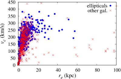
Figure 1: Circular velocity $v_{c}$ as a function of effective radius $r_{e}$ for a sample of galaxies listed in Table 1 from [29].

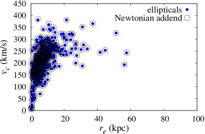
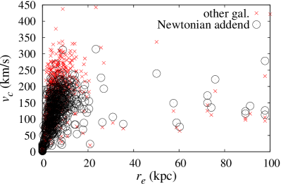
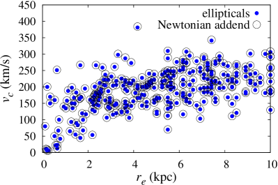
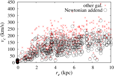
Figure 2: (left): Circular velocity $v_{c}$ as a function of effective radius $r_{e}$ for elliptical galaxies (full circles) and their Newtonian circular velocity $v_{c,N}(r_{e})$ (open circles). (right): $v_{c}$($r_{e}$) for other galaxies (crosses) and their Newtonian circular velocity $v_{c,N}(r_{e})$ (open circles). Bottom panel shows a zoomed part of the figure, for $r_{e}$ less than 10 kpc. Data are from [29].

The FP can be written in the form [2]:

$$log(r_{e})=a\times log(v)+b\times log(I_{e})+c,$$ (10)

where $r_{e}$ is the effective radius (or half-light radius, within which the half of galaxy’s luminosity is contained), $v$ is the central velocity dispersion, and $I_{e}$ is the mean surface brightness within the effective radius. In principle, this formula can summarize the kinematical, morphological and photometric features of a given object represented as a point in the parameter space $\{r_{e},v,I_{e}\}$. The velocity $v$ assumes the meaning of the characteristic velocity of the self-gravitating system that we are considering. In the case of elliptical galaxies, $v=\sigma_{0}$ that is the central velocity dispersion [34]. This means that kinematics is not dominated by well defined circular velocities of orbiting objects (stars) as in the case of spiral galaxies (called ”cold systems”) but we need a velocity distribution as in thermodynamics (elliptical galaxies are called ”hot systems” where a characteristic temperature $T$ is related to $\sigma_{0}$). More in detail, most elliptical galaxies exhibit little or no rotation. Their stars have random velocities along the line of sight whose root mean square dispersion $\sigma_{0}$ can be measured from the Doppler broadening of spectral lines [34].

The constant $c$ strictly depends on the morphology and the homology properties of the systems [5, 6].

Finally, it is worth noticing that $r_{e}$ is typically of the order 3 kpc for bright ellipticals and smaller for fainter galaxies [34, 35]. It is assumed that the largest luminous mass fraction of the galaxy is concentrated within $r_{e}$ so that it can be considered as a typical gravitational radius, being a galaxy a diffuse system without a defined boundary. We want to show that the FP could be modulated by $f(R)$, and in such a way the issues related to DM could be completely reproduced.

In this paper, we use the data given in Table I of [29], which are the result of the collected efforts of many astronomers over the years (as summarized in the table’s explanation - available among the source files of its arxiv version). We want to recover FP using $f(R)$ gravity, which means to find connection between the parameters of FP equation and parameters of the potential in Eq. (6). In this sense, the three addends of Eq. (10) can be connected to the above $f(R)$ gravitational potential in order to find out an equation tying together theoretical and observational quantities. Specifically:

• the addend with $r_{e}$ means that we need a term relating $r_{e}$ and $r_{c}$ in the above equation;

• the addend with $v$ means that we need a term relating the velocity dispersion $\sigma_{0}$ and $v_{vir}$, where $v_{vir}$ is the virial velocity in $f(R)$;

• addend with $I_{e}$ means that we need a term relating $I_{e}$ and $r_{c}$ (through the $r_{c}/r_{e}$ ratio).

Addend with $r_{e}$

We use columns (5), (6) and (7) of Table 1 in [29], as well as the notation for circular velocity $v_{c}$ from that table that, for ellipticals, is $v_{c}$ = $\sigma_{0}$, to plot the graphic $v_{c}(r_{e})$ for ellipticals and for other galaxies (see Fig. 1).

Starting from Eq. (9), the rotation curve for extended systems in $R^{n}$ gravity, generated by spherically symmetric mass distribution, can be recast in the form:

$$v_{c}^{2}\left(r\right)=\frac{v_{c,N}^{2}\left(r\right)}{2}+\frac{r}{2}\frac{\partial{\Phi_{c}}}{\partial r},$$ (11)

with $v_{c,N}^{2}=\dfrac{GM(r)}{r}$ being the Newtonian rotation curve and $G=4.302\times 10^{-6}\dfrac{kpc}{M_{sun}}\left(\dfrac{km}{s}\right)^{2}$ the gravitational constant. $\Phi_{c}(r)$ is the correction term of $R^{n}$ gravity potential for spherically symmetric extended systems (see also [23] for a discussion). According to Eq. (11), in the case when $r_{c}$ is proportional to $r_{e}$, the second addend becomes zero, so the circular velocity becomes exactly the Newtonian circular velocity $v_{c,N}$ (see Fig. 2). However, the velocity dispersion $\sigma_{0}$ of elliptical galaxies is equal to their circular velocity $v_{c}$ at the effective radius $r_{e}$, i.e. the following expression holds:

$$\sigma_{0}=v_{c}(r_{e}),$$ (12)

while this is not the case for non-ellipticals [34].

Let us assume now the reasonable assumption that the gravitational radius $r_{c}$ is proportional, for elliptical galaxies, to the effective radius:

$$r_{c}\propto r_{e}.$$ (13)

This assumption is supported by the above empirical definition of $r_{e}$ which can be considered a ”gravitational radius” enclosing the largest amount of luminous gravitating mass of the galaxy. Assuming the relation (13) means that the theoretical gravitational radius $r_{c}$ and the observational gravitational radius $r_{e}$ must be related and eventually coincide, as in the case of Eq. (12) where the velocity dispersion $\sigma_{0}$ coincides with the circular velocity $v_{c}$ at the boundary defined by $r_{e}$.

Using (13) we have $\xi\left({{r_{e}}}\right)=\dfrac{{{r_{c}}}}{{{r_{e}}}}=const$, so the integrals (23) and (24) in [23], i.e. $I_{1}\left({r_{e}}\right)$ and $I_{2}\left({r_{e}}\right)$, do not depend on $r$. This means that the correction term of the gravitational potential $\Phi_{c}\left({r_{e}}\right)$ also does not depend on $r$. Therefore, it is $\dfrac{\partial{\Phi_{c}\left({r_{e}}\right)}}{\partial r}=0\Rightarrow v_{c,corr}=0$, and by (11) and (12), we have:

$$\sigma_{0}=\dfrac{v_{c,N}\left(r_{e}\right)}{\sqrt{2}},$$ (14)

with $v_{c,N}$ being the Newtonian circular velocity and $v_{c,corr}$ the correction term coming from $R^{n}$ gravity. In other words, under the condition (13), $R^{n}$ gravity gives the same $\sigma_{0}$ for elliptical galaxies as in Newtonian case. However, this is not true for non-ellipticals, since in that case $v_{c,corr}\neq 0$ (see [34] for a detailed discussion).

Addend with $v$

We can deal with objects in FP as virialized systems. In that sense, we can take for virial velocity in $R^{n}$: $v_{vir}$ = $v_{c}$. As for ellipticals (see the above discussion and explanation for Table 1 in [29]) $v_{c}$ = $\sigma_{0}$, directly we have the connection between $\sigma_{0}$ and $v_{vir}$, i.e. their equality.

Addend with $I_{e}$

Correlation of this addend with $r_{c}$ is reflected through the coefficient $b$ of FP in Eq. (10) or, in the other empirical form, $r_{e}\sim I_{e}^{\,b}v^{\,a}$ given in [5, 6]. In other words, this means that being $r_{c}$ related to $r_{e}$ through Eq.(13), also $r_{c}$ is related to $I_{e}$. In general, this means that photometric quantities like $I_{e}$ are related to gravitational parameters like $r_{c}$.

In [5], it is derived the FP of elliptical galaxies, i.e. $a$ and $b$ are calculated as coefficients of the FP equation (using the Virgo Cluster elliptical galaxies as a sample). The empirical result is $a=1.4,b=-0.85$. The test for our method is recovering this profile (see Fig. 3). In other words, starting from the gravitational potential derived from $f(R)$ gravity, the values of parameters $a$ and $b$ as deduced from observations, have to be consistently reproduced.

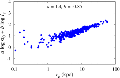
Figure 3: Fundamental plane equation for observed values of effective radius $r_{e}$, velocity dispersion $\sigma_{0}$ and mean surface brightness within the effective radius $I_{e}$, and for values of $a$ and $b$ coefficients taken from [5]: $a=1.4$ and $b=-0.85$.

4 The empirical fundamental plane reproduced by $f(R)$ gravity

The theoretical circular velocity in extended spherically symmetric systems is calculated by using Eq. (11), and taking into account the so called Hernquist profile for density distribution [30]. This velocity is connected to $r_{c}$ and $\beta$ as given in Eq. (9). Using these theoretical values for $v_{c}$, and the observed values for $r_{e}$ and $I_{e}$, it is possible to calculate a 3D fit of the FP, and as result, to obtain the coefficients of FP equation, that is $a$, $b$ and $c$. The method consists with the procedure that Eq. (10) is fitted with

$$z(x,y)=ax+by+c\,,$$ (15)

where $x=\mathrm{log}(v)$, $y=\mathrm{log}(I_{e})$ and $z=\mathrm{log}(r_{e})$. Then one can calculate a table of values comparing the couples ($r_{c}$, $\beta$) vs ($a$,$b$), with absolute errors for $a$, $b$, $c$, and $\chi^{2}$ for the fit (see Tables 1 and 2). In such a way, we reproduce the FP generated by the power law $f(R)$ gravity without considering the presence of dark matter in galaxies. In other words, the parameters $r_{c}$ (specifically the ratio $r_{c}/r_{e}$) and $\beta$ are used to calculate the terms $x$ and $y$ of Eq.(15). Once this procedure is performed, the values of $a$ and $b$ that satisfy Eq.(10) are compared with the $a$ and $b$ values experimentally obtained by observations [5, 6]. The final goal is to reproduce the observational FP only by parameters coming from the weak field limit of power-law $f(R)$ gravity.

Some important remarks are necessary at this point. Low Surface Brightness galaxies and galaxy clusters give a non vanishing beta when they are analyzed without including DM. Solar System data resulted with tight constraints on $\beta$, and in the case of the perihelion precession of Mercury gave $\beta\approx 0$, [18, 31], practically recovering GR. However, constraints derived from slightly larger scales, such as those coming from Cassini mission, gave $\beta\approx 2\times 10^{-6}$ as upper bound (see [32] and references therein). Although GR is well working on these scales, some more recent studies indicate that it is not the case for the larger galactic scales where significantly larger values of $\beta$ can be obtained, showing that effects of $R^{n}$ gravity could start to work and should be taken into account at such scales. For example, as shown in [33], the value of this parameter which gives the best fit of the observed orbit of S2 star around the Galactic Centre is $\beta\approx 0.01$, i.e. four orders of magnitude larger than the previously mentioned upper bound in the case of Solar System. Besides, studies on Low Surface Brightness galaxies and galaxy clusters indicate even much larger value $\beta=0.817$ (see [23, 24, 26]). The cases of Low Surface Brightness galaxies and galaxy clusters are extremely important in order to point out the breaking of gravity scale invariance at galactic scales. Specifically, the fact that $\beta\simeq 0$ inside the Solar System and significantly different from zero at galactic scales is the feature characterizing this issue. For example, as discussed in detail in [23, 24] by using the data reported in [36], the theoretical rotation curve of Low Surface Brightness galaxies can be modeled as a function of three unknown quantities, namely the stellar $M/L$ ratio $\Upsilon_{\star}$ and the two theory parameters $(\beta,r_{c})$. Actually, in [23], the fitting parameter has been $\log{r_{c}}$ rather than $r_{c}$ (in kpc) since this is a more manageable quantity that makes it possible to explore a larger range of parameter space. Moreover, the gas mass fraction $f_{g}$, rather than $\Upsilon_{\star}$ is another important fitting quantity [24] since the range for $f_{g}$ is clearly defined, while this is not for $\Upsilon_{\star}$. The two quantities are easily related as follows :

$$f_{g}=\frac{M_{g}}{M_{g}+M_{d}}\iff\Upsilon_{\star}=\frac{(1-f_{g})M_{g}}{f_{g}L_{d}}$$ (16)

with $M_{g}=1.4M_{HI}$ the gas (HI + He) mass, $M_{d}=\Upsilon_{\star}L_{d}$ and $L_{d}=2\pi I_{0}R_{d}^{2}$ the disk total mass and luminosity. To constrain the parameters $(\beta,\log{r_{c}},f_{g})$, the following merit function has been minimized :

$$\chi^{2}({\bf p})=\sum_{i=1}^{N}{\left[\frac{v_{c,th}(r_{i})-v_{c,obs}(r_{i})}{\sigma_{i}}\right]^{2}}$$ (17)

where the sum is over the $N$ observed points. While using the smoothed data helps in better adjusting the theoretical and observed rotation curves, the smoothing procedure implies that the errors $\sigma_{i}$ on each point are non-Gaussian distributed since they also take into account systematic misalignments between HI and H$\alpha$ measurements and other effects leading to a conservative overestimate of the true uncertainties (see the discussion in [36] for further details). As a consequence, one does not expect that $\chi^{2}/dof\simeq 1$ for the best fit model (with $dof=N-3$ the number of degrees of freedom), but one can still compare different models on the basis of the $\chi^{2}$ values. In particular, the uncertainties on the model parameters have estimated exploring the contours of equal $\Delta\chi^{2}=\chi^{2}-\chi^{2}_{min}$ in the parameter space. Considering the observational data in [36] the best fit value for Low Surface Brightness galaxies is $\beta=0.817$. Similar procedures can be adopted for giant elliptical galaxies [25] and galaxy clusters [26]. The result is always that consistent deviations from Newtonian gravity (working in excellent way at Solar System scales) are found at galactic scales.

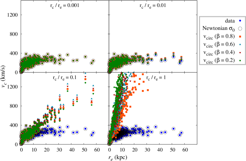
Figure 4: Circular velocity $v_{c}$ as a function of effective radius $r_{e}$ for elliptical galaxies, for different values of ratio between $R^{n}$ gravity scale-length and effective radius $r_{c}/r_{e}$: 0.001, 0.01, 0.1 and 1. For every of these ratios, the four values of $\beta$ are presented: 0.2, 0.4, 0.6 and 0.8. Notice: all $v_{c}$ values we calculated, except for blue full circles which are data given in Table 1 from [29].

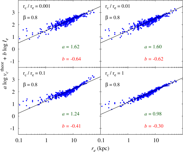
Figure 5: Fundamental plane of elliptical galaxies with calculated circular velocity $v_{c}^{theor}$ and observed effective radius $r_{e}$ and mean surface brightness within the effective radius $I_{e}$. For each given pair of $R^{n}$ gravity parameters ($r_{c}$, $\beta$), i.e. for the certain cases $r_{c}/r_{e}$ = 0.001, 0.01, 0.1 and 1, and $\beta$ = 0.8, we present calculated FP coefficients ($a$, $b$). Black solid line is result of 3D fit of FP.

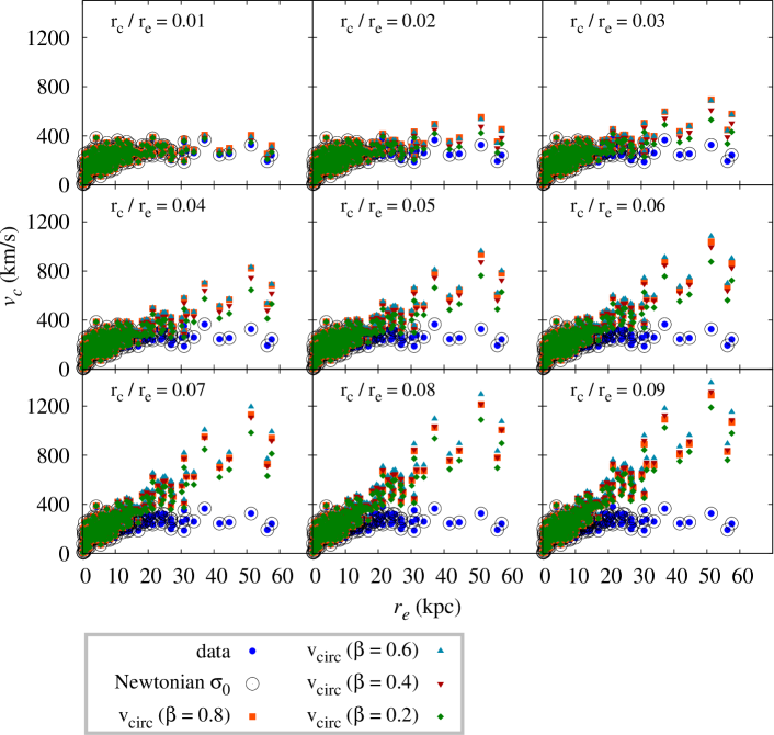
Figure 6: The same as in Fig. 4, but for the following $r_{c}/r_{e}$ ratios: 0.01, 0.02, 0.03, 0.04, 0.05, 0.06, 0.07, 0.08 and 0.09.

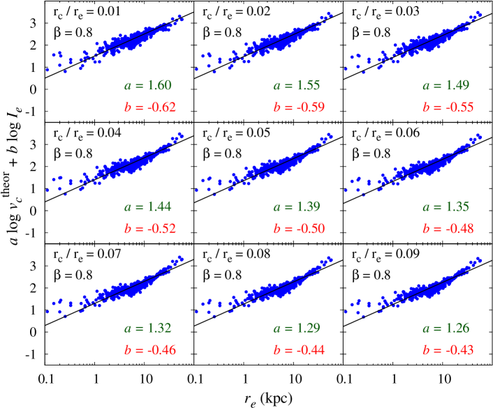
Figure 7: The same as in Fig. 5, but for the following $r_{c}/r_{e}$ ratios: 0.01, 0.02, 0.03, 0.04, 0.05, 0.06, 0.07, 0.08 and 0.09.

All these results imply that gravity, most likely, could be not a scale invariant interaction, and thus $\beta$ could have different values depending on the scale of a gravitating system. Taking this into account, as well as the fact that the effective galactic radii $r_{e}$ with size of $\sim 3$ kpc in average (see [34]), have the significant influence on FP, it is expected that $\beta$ should be much larger in the case of FP than for S2 star orbit around Galactic Centre (which size is on the order of 1 mpc), and close to the values for the rotation curves of spiral galaxies. Therefore, we investigated the cases where $\beta$ ranges between 0.2 and 0.8 (see Tables 1-2 and Figs. 4-8). In summary, if further evidences will be found in this direction, these could indicate that the straightforward extrapolation of Solar System results to any astrophysical and cosmological scale is an approach that has to be carefully revised.

Regarding the characteristic radius $r_{c}$ of $R^{n}$ gravity, we investigated its potential dependence on the effective radius $r_{e}$. For this purpose, we assumed that these two radii are proportional and tested their different ratios. The obtained results are presented in Tables 1-2 and Figs. 1-8. It can be seen that for $r_{c}/r_{e}\approx 0.05$, the coefficient $a$ is exactly like in [5]. The coefficient $b$ has similar but not exactly the same value. However we calculated $v_{c}$ only theoretically. For $I_{e}$, we are considering observed values but, in any case, the agreement with data is quite good (see the middle panel of Fig. 7). As discussed in Sec. 3, photometric observations gives $I_{e}$ [34] and this allow to infer the value of $r_{e}$ (and then $r_{c}$ in our case). The value of $v_{c}$ depends on the self-gravitating system and, for ellipticals, from the observed $\sigma_{0}$ calculated at $r_{e}$. In other words, FP can be constructed by a set of bivariate correlations connecting some of the properties of (elliptical) galaxies or self-gravitating systems, including some characteristic radius (e.g. $r_{e}$), luminosity, mass, velocity dispersion, surface brightness, and so on. In its standard formulation, it is expressed as a relation between the effective radius, average surface brightness and central velocity dispersion for normal elliptical galaxies. Any of these three parameters can be estimated from the other two. The result is a plane embedded in a three-dimensional space [5, 6].

By these considerations and results, we can state that DM effects in FP can be reasonably reproduced by power law $f(R)$ gravity. This is not surprising considering that similar results hold for single galaxies [23, 24]. Also, in Figs. 4 and 6 we present the calculated values of $v_{c}$ as a function of effective radius $r_{e}$ for elliptical galaxies, for different values of $r_{c}/r_{e}$ ratio (from 0.001 to 1), and the four values of $\beta$: 0.2, 0.4, 0.6 and 0.8. While in Fig. 4 we use the following certain $r_{c}/r_{e}$ ratios: 0.001, 0.01, 0.1 and 1 (like some of them in Table 1), in Fig. 6 the $r_{c}/r_{e}$ ratios are: 0.01, 0.02, 0.03, 0.04, 0.05, 0.06, 0.07, 0.08 and 0.09 (like in Table 2). It can be noticed that $r_{c}/r_{e}$ has more influence on $v_{c}$ than $\beta$. From Fig. 4, it is noticeable that it is good agreement between observations and the calculations for smaller values of $r_{c}/r_{e}$ of the order of magnitudes $10^{-3}\div 10^{-2}$, and then the agreement is good for all $\beta$ between 0.2 and 0.8. With increasing of that ratio, for better agreement, value of $\beta$ parameter has to decrease.

For a better insight in these results, we present the graphs with the FP of elliptical galaxies with calculated $v_{c}$ and observed $r_{e}$ and $I_{e}$ (Figs. 5 and 7). For certain values of $r_{c}/r_{e}$ and $\beta$, we present calculated FP coefficients ($a$, $b$). Also, the 3D fit of FP is performed. From Fig. 5 it can be seen that for relatively small values of $r_{c}/r_{e}$, the change of coefficients $a$ and $b$ with changing of that ratio is very small, even when $r_{c}/r_{e}$ is increased ten times. But for larger value of $r_{c}/r_{e}$, change of this ratio has greater influence on parameters $a$ and $b$. Fig. 7 is useful for comparing coefficients $a$ and $b$ which we derived from $f(R)$ gravity, with the ones deduced from observations. When compare to empirical result from [5], it is noticeable that the most similar values of ($a$,$b$) correspond to $r_{c}/r_{e}$ interval [0.04,0.06].

Table 1: Values of $R^{n}$ gravity parameters ($r_{c}$, $\beta$) and the corresponding FP coefficients ($a$, $b$, $c$) calculated by 3D fit of FP equation, with given $\chi^{2}$ for each fit. The chosen ratios between $R^{n}$ gravity scale-length and effective radius are $r_{c}/r_{e}$ = 0.001, 0.01, 0.1 and 1. For every of these ratios, the following four values of $\beta$ are taken: 0.2, 0.4, 0.6 and 0.8.

$r_{c}/r_{e}$	$\beta$	$a$	$b$	$c$	$\chi^{2}$
1	0.2	0.861 $\pm$ 0.012	-0.280 $\pm$ 0.012	-1.097 $\pm$ 0.045	0.00934
1	0.4	0.881 $\pm$ 0.013	-0.282 $\pm$ 0.013	-1.100 $\pm$ 0.047	0.01002
1	0.6	0.912 $\pm$ 0.014	-0.286 $\pm$ 0.013	-1.109 $\pm$ 0.049	0.01108
1	0.8	0.976 $\pm$ 0.016	-0.303 $\pm$ 0.014	-1.137 $\pm$ 0.054	0.01317
0.5	0.2	0.905 $\pm$ 0.015	-0.267 $\pm$ 0.014	-1.071 $\pm$ 0.053	0.01305
0.5	0.4	0.918 $\pm$ 0.015	-0.270 $\pm$ 0.015	-1.075 $\pm$ 0.054	0.01361
0.5	0.6	0.941 $\pm$ 0.016	-0.277 $\pm$ 0.015	-1.085 $\pm$ 0.056	0.01459
0.5	0.8	1.000 $\pm$ 0.019	-0.300 $\pm$ 0.016	-1.116 $\pm$ 0.061	0.01658
0.1	0.2	1.249 $\pm$ 0.029	-0.420 $\pm$ 0.019	-1.246 $\pm$ 0.079	0.02490
0.1	0.4	1.217 $\pm$ 0.028	-0.404 $\pm$ 0.019	-1.219 $\pm$ 0.078	0.02491
0.1	0.6	1.204 $\pm$ 0.028	-0.397 $\pm$ 0.019	-1.206 $\pm$ 0.078	0.02499
0.1	0.8	1.238 $\pm$ 0.029	-0.415 $\pm$ 0.019	-1.234 $\pm$ 0.079	0.02523
0.05	0.2	1.454 $\pm$ 0.034	-0.530 $\pm$ 0.020	-1.411 $\pm$ 0.084	0.02579
0.05	0.4	1.412 $\pm$ 0.034	-0.507 $\pm$ 0.020	-1.376 $\pm$ 0.083	0.02592
0.05	0.6	1.383 $\pm$ 0.033	-0.492 $\pm$ 0.020	-1.349 $\pm$ 0.083	0.02606
0.05	0.8	1.394 $\pm$ 0.033	-0.498 $\pm$ 0.020	-1.358 $\pm$ 0.083	0.02608
0.01	0.2	1.616 $\pm$ 0.040	-0.639 $\pm$ 0.021	-1.504 $\pm$ 0.089	0.02749
0.01	0.4	1.611 $\pm$ 0.039	-0.634 $\pm$ 0.021	-1.505 $\pm$ 0.088	0.02729
0.01	0.6	1.605 $\pm$ 0.039	-0.628 $\pm$ 0.021	-1.505 $\pm$ 0.088	0.02706
0.01	0.8	1.600 $\pm$ 0.039	-0.624 $\pm$ 0.020	-1.504 $\pm$ 0.088	0.02694
0.005	0.2	1.620 $\pm$ 0.040	-0.643 $\pm$ 0.021	-1.502 $\pm$ 0.089	0.02773
0.005	0.4	1.619 $\pm$ 0.040	-0.642 $\pm$ 0.021	-1.503 $\pm$ 0.089	0.02767
0.005	0.6	1.617 $\pm$ 0.040	-0.640 $\pm$ 0.021	-1.503 $\pm$ 0.089	0.02757
0.005	0.8	1.616 $\pm$ 0.040	-0.639 $\pm$ 0.021	-1.504 $\pm$ 0.089	0.02749
0.001	0.2	1.620 $\pm$ 0.040	-0.644 $\pm$ 0.021	-1.501 $\pm$ 0.089	0.02779
0.001	0.4	1.620 $\pm$ 0.040	-0.644 $\pm$ 0.021	-1.501 $\pm$ 0.089	0.02779
0.001	0.6	1.620 $\pm$ 0.040	-0.644 $\pm$ 0.021	-1.502 $\pm$ 0.089	0.02778
0.001	0.8	1.620 $\pm$ 0.040	-0.644 $\pm$ 0.021	-1.502 $\pm$ 0.089	0.02778

Table 2: The same as in Table 1, but for the following $r_{c}/r_{e}$ ratios: 0.01, 0.02, 0.03, 0.04, 0.05, 0.06, 0.07, 0.08 and 0.09.

$r_{c}/r_{e}$	$\beta$	$a$	$b$	$c$	$\chi^{2}$
0.09	0.2	1.282 $\pm$ 0.030	-0.437 $\pm$ 0.020	-1.272 $\pm$ 0.080	0.02519
0.09	0.4	1.247 $\pm$ 0.029	-0.419 $\pm$ 0.019	-1.241 $\pm$ 0.079	0.02524
0.09	0.6	1.231 $\pm$ 0.029	-0.411 $\pm$ 0.020	-1.226 $\pm$ 0.079	0.02532
0.09	0.8	1.261 $\pm$ 0.030	-0.427 $\pm$ 0.020	-1.251 $\pm$ 0.080	0.02549
0.08	0.2	1.319 $\pm$ 0.031	-0.457 $\pm$ 0.020	-1.301 $\pm$ 0.081	0.02542
0.08	0.4	1.281 $\pm$ 0.030	-0.437 $\pm$ 0.020	-1.268 $\pm$ 0.080	0.02551
0.08	0.6	1.261 $\pm$ 0.030	-0.427 $\pm$ 0.020	-1.250 $\pm$ 0.080	0.02561
0.08	0.8	1.288 $\pm$ 0.031	-0.441 $\pm$ 0.020	-1.272 $\pm$ 0.081	0.02571
0.07	0.2	1.360 $\pm$ 0.032	-0.478 $\pm$ 0.020	-1.335 $\pm$ 0.082	0.02559
0.07	0.4	1.319 $\pm$ 0.031	-0.457 $\pm$ 0.031	-1.299 $\pm$ 0.081	0.02572
0.07	0.6	1.296 $\pm$ 0.031	-0.445 $\pm$ 0.020	-1.277 $\pm$ 0.080	0.02584
0.07	0.8	1.318 $\pm$ 0.031	-0.457 $\pm$ 0.020	-1.296 $\pm$ 0.081	0.02589
0.06	0.2	1.405 $\pm$ 0.033	-0.503 $\pm$ 0.020	-1.371 $\pm$ 0.083	0.02570
0.06	0.4	1.363 $\pm$ 0.032	-0.481 $\pm$ 0.020	-1.335 $\pm$ 0.082	0.02585
0.06	0.6	1.336 $\pm$ 0.032	-0.467 $\pm$ 0.020	-1.311 $\pm$ 0.082	0.02599
0.06	0.8	1.353 $\pm$ 0.032	-0.476 $\pm$ 0.020	-1.325 $\pm$ 0.082	0.02601
0.05	0.2	1.454 $\pm$ 0.034	-0.530 $\pm$ 0.020	-1.411 $\pm$ 0.084	0.02579
0.05	0.4	1.412 $\pm$ 0.034	-0.507 $\pm$ 0.020	-1.376 $\pm$ 0.083	0.02592
0.05	0.6	1.383 $\pm$ 0.033	-0.492 $\pm$ 0.020	-1.349 $\pm$ 0.083	0.02606
0.05	0.8	1.394 $\pm$ 0.033	-0.498 $\pm$ 0.020	-1.358 $\pm$ 0.083	0.02608
0.04	0.2	1.504 $\pm$ 0.034	-0.560 $\pm$ 0.020	-1.449 $\pm$ 0.085	0.02592
0.04	0.4	1.466 $\pm$ 0.034	-0.538 $\pm$ 0.020	-1.420 $\pm$ 0.084	0.02596
0.04	0.6	1.436 $\pm$ 0.034	-0.521 $\pm$ 0.020	-1.394 $\pm$ 0.083	0.02607
0.04	0.8	1.440 $\pm$ 0.034	-0.523 $\pm$ 0.020	-1.397 $\pm$ 0.084	0.02609
0.03	0.2	1.553 $\pm$ 0.037	-0.590 $\pm$ 0.020	-1.482 $\pm$ 0.086	0.02620
0.03	0.4	1.523 $\pm$ 0.036	-0.571 $\pm$ 0.020	-1.462 $\pm$ 0.085	0.02608
0.03	0.6	1.495 $\pm$ 0.036	-0.555 $\pm$ 0.020	-1.441 $\pm$ 0.085	0.02609
0.03	0.8	1.493 $\pm$ 0.036	-0.554 $\pm$ 0.0120	-1.439 $\pm$ 0.085	0.02611
0.02	0.2	1.593 $\pm$ 0.039	-0.619 $\pm$ 0.021	-1.502 $\pm$ 0.087	0.02675
0.02	0.4	1.575 $\pm$ 0.038	-0.606 $\pm$ 0.021	-1.494 $\pm$ 0.087	0.02648
0.02	0.6	1.556 $\pm$ 0.037	-0.592 $\pm$ 0.021	-1.484 $\pm$ 0.086	0.02631
0.02	0.8	1.550 $\pm$ 0.037	-0.588 $\pm$ 0.020	-1.480 $\pm$ 0.086	0.02629
0.01	0.2	1.616 $\pm$ 0.040	-0.639 $\pm$ 0.021	-1.504 $\pm$ 0.089	0.02749
0.01	0.4	1.611 $\pm$ 0.039	-0.634 $\pm$ 0.021	-1.505 $\pm$ 0.088	0.02729
0.01	0.6	1.605 $\pm$ 0.039	-0.628 $\pm$ 0.021	-1.505 $\pm$ 0.088	0.02706
0.01	0.8	1.600 $\pm$ 0.039	-0.624 $\pm$ 0.020	-1.504 $\pm$ 0.088	0.02694

Table 3: Results of the fitting of the empirical function $f(x,\beta)=u\cdot\left(\dfrac{e^{-vx}-1}{(1+\beta)^{w}}+2\right)$ to the values of $a(x,\beta)$, $b(x,\beta)$ and $c(x,\beta)$ from Table 1, where $x=r_{c}/r_{e}$.

$f(x,\beta)$	$u$	$v$	$w$
$a(x,\beta)$	0.827 $\pm$ 0.004	8.1 $\pm$ 0.5	0.28 $\pm$ 0.04
$b(x,\beta)$	-0.330 $\pm$ 0.003	10.9 $\pm$ 0.7	-0.27 $\pm$ 0.04
$c(x,\beta)$	-0.767 $\pm$ 0.009	8.5 $\pm$ 1.5	1.28 $\pm$ 0.14

The next step is to find out the functional relations: $a$ = $a(r_{c},\beta)$, $b$ = $b(r_{c},\beta)$ and $c$ = $c(r_{c},\beta)$. Using data obtained from Table 1, we found that $a$, $b$ and $c$ satisfy the following empirical dependencies on two variables: $f(x,\beta)=u\cdot\left(\dfrac{e^{-vx}-1}{(1+\beta)^{w}}+2\right)$, with $x=r_{c}/r_{e}$. The coefficients of these empirical dependencies are obtained using least square fit method. We obtained that there is a very strong dependence on $r_{c}$ in the form of the exponential functions and a weak dependence on $\beta$ (see Table 3 and Fig. 8). We expected the strong dependence on $r_{c}$ and a weak on $\beta$ because, like we mentioned in Sec. 2, $\beta$ should represent a universal constant and $r_{c}$ depends on the system’s dynamical properties. From Fig. 8 it can be seen that $f(x,\beta)$ describes $a$ and $b$ very well, in the whole range of $r_{c}/r_{e}$ from 0.001 to 1, and for all studied values of $\beta$.

As reported in Sec. 3, the value of parameter $c$ depends on the morphology and the homology properties of the sample of self-gravitating systems used to construct the FP [5]. In other words, considering ellipticals, spirals, dwarfs and so on gives different values for $c$. Geometrically, $c$ fixes the intersection of FP with the axes of parameter space. Furthermore, morphology has a main role in determining the DM content of systems so parameters like $\beta$ and $r_{c}$, that correct the Newtonian potential, can be influenced by the observed values of $c$ [23, 25]. In particular, the observational FP reported in [5, 6] for ellipticals, is well reproduced in the framework of power law $f(R)$ gravity as soon as $\beta\simeq 0.8$ and $r_{c}/r_{e}\simeq 0.05$. In such a case, the parameters $a,b,c$ of Eq.(10) are in excellent agreement with observations without considering the presence of DM.

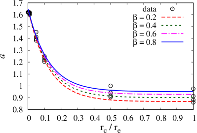
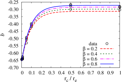
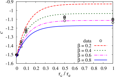
Figure 8: Fits of the empirical function $f(x,\beta)=u\cdot\left(\dfrac{e^{-vx}-1}{(1+\beta)^{w}}+2\right)$ to the values of $a(x,\beta)$, $b(x,\beta)$ and $c(x,\beta)$ from Table 1, respectively, where $x=r_{c}/r_{e}$.

5 Conclusions

In recent years DM as well as dark energy are become the main issues in cosmology and astrophysics because also if their effects are observed at almost every scale, their detection as new fundamental particles remains very elusive and complicated. In other words, also if the macroscopic, large scale (infrared) effects of these components are clearly evident, the quantum physics counterpart (new particles at ultraviolet scales) cannot be easily found out. This puzzling situation could be overcome by considering the gravitational sector and the possibility to extend General Relativity at large scales by retaining its positive results at local and Solar System scales. Addressing astrophysical systems and the whole Universe evolution by modified or extended gravity is a compelling approach with respect to introducing the Dark Side in the cosmological dynamics. In this perspective, FP can play a major role as test bed for these theories in view of explaining galactic structures without DM.

Specifically, FP is a formidable tool in extragalactic astrophysics used to study the evolution and the dynamics of self-gravitating systems like elliptical galaxies, bulges of spiral galaxies, globular clusters and so on. In some sense, the role of FP for galaxies could be similar to the Herzsprung-Russell diagram for stars: a bivariate sequence of characteristic parameters assigns the position and then the evolution on a sort of suitable phase-space of hot stellar systems. However, as reported in [5] and [6], a quite large amount of physical processes can affect the shape (tightness) and the position (tilt) of FP in this phase-space. In particular, the presence of DM strongly affects the position of objects in FP determining also their evolution.

In this paper, we consider the possibility to reproduce the FP of galaxies (in particular elliptical galaxies) adopting the corrected gravitational potential coming out as solution of power law $f(R)=f_{0}R^{n}$ gravity, a straightforward extension of Einstein’s General Relativity related to the existence of Noether symmetries that select the value of $n$ [19, 20]. In particular, we have shown that $R^{n}$ gravity gives the same $\sigma_{0}$ for elliptical galaxies as in the Newtonian case, but for spiral galaxies (and other non-ellipticals) it is not the case. We obtained that for elliptical galaxies the characteristic radius $r_{c}$ is proportional to the effective radius $r_{e}$, more precise $r_{c}\approx 0.05\,r_{e}$ gives the best fit with data. An important point has to be stressed again at this point. The effective radius $r_{e}$, observationally derived from photometry, actually is a gravitational radius in the sense that its value is determined by the self-gravitating luminous matter content in the inner part of the elliptical galaxy. As discussed in [34], it can be defined for any spheroidal system where gravity is the dominant interaction. The previous assumption that $r_{c}\propto r_{e}$ is motivated by the fact that also $r_{c}$ is a gravitational radius that comes out from the theory. Since observational FP gives $r_{c}/r_{e}\simeq 0.05$, this can be considered as a sort of consistency check that both (observational) $r_{e}$ and (theoretical) $r_{c}$ are gravitational radii.

We want to stress again that $r_{c}$ radius is a gravitational radius, and it comes out from the fact that a fourth order theory of gravity, like $f(R)$, gives a further gravitational radius than the Schwarzschild one. As shown in [19], this further radius comes directly from the presence of a Noether symmetry. Considering the definition of $r_{e}$, we are saying that the effective radius (defined photometrically as the radius containing half of the luminosity of a galaxy) is, in some sense, led by gravity.

In summary, our analysis shows that:

1. the observed FP for elliptical galaxies can be reproduced by $R^{n}$ gravity. In particular, we have shown that $R^{n}$ gravity gives the same $\sigma_{0}$ for elliptical galaxies as in the Newtonian case;

2. the assumption that the characteristic radius $r_{c}$ of $R^{n}$gravity is proportional to the effective radius $r_{e}$ of elliptical galaxies can be probed: we probed the ratio of this quantities and that, under this assumption, f(R) is able to reproduce the FP. Thus, if we take into account the definition of $r_{e}$, this indicates that the effective radius (defined photometrically as the radius containing half of the luminosity of a galaxy) is led by gravity;

3. in the range $r_{c}/r_{e}\sim 10^{-3}\div 10^{-2}$, the values of $\beta$, which are deduced from the LSB galaxies [23] and galaxy clusters [26], are in agreement with FP of elliptical galaxies. In other words, the same range of values of $r_{c}$ and $\beta$ work at galactic scales. The fact that these values are larger than the corresponding values obtained from the observational data at smaller scales, such as those from Solar System, may indicate that gravity is not a scale invariant interaction. This point deserves some comment. In [24], the analysis of Low Surface Brightness galaxies, performed in [23], has been extended to a wider class of objects containing also High Surface Brightness galaxies, while in [37] the baryonic Tully-Fisher relation has also been adopted besides the Low Surface galaxies sample. In the first case, the result was $\beta=0.7\pm 0.25$, in the second case, it was $\beta=0.58\pm 0.15$. Both cases are consistent with the present result $\beta\sim 0.8$ but the lesson is that morphology and homology determine corrections to the Newtonian potential. On the other hand, the result $\beta\simeq 0$, from Cassini and other Solar System experiments, clearly means that at local scales such corrections are not relevant;

4. the further gravitational radius $r_{c}$ is related to the radius of galactic bulges or the hot spherical component of galaxies. In the present case, it is related to $r_{e}$ that is the effective radius of ellipticals.

In conclusion, the observed empirical FP can be reproduced by $f(R)$ gravity without assuming DM while the photometry of the systems is led by the gravitational corrections. These preliminary results can be improved considering detailed samples of data and different classes of objects.

A final remark is now necessary. As we said above, the reported results seem to point out that, in absence of dark matter, gravity is not a scale-invariant interaction. This means that constraints working at Solar System level for General Relativity could not be simply extrapolated at any astrophysical and cosmological scale. Besides, the presence of Noether symmetries could rule the strength and the shape of gravitational interaction at different scales. In our case, the couple of parameters $r_{c}$ and $\beta$ indicate if given self-gravitating systems (in this case elliptical galaxies) sit or not on FP. However further and detailed investigations are necessary to confirm this delicate statement.

Acknowledgments

We wish to acknowledge the support by the Ministry of Education, Science and Technological Development of the Republic of Serbia, through the project 176003 (V.B.J., P.J. and D.B.), and Istituto Nazionale di Fisica Nucleare, Sezione di Napoli, Italy, iniziative specifiche TEONGRAV and QGSKY (S.C.). The authors also acknowledge the support of the Bilateral Cooperation between Serbia and Italy 451-03-01231/2015-09/1 ”Testing Extended Theories of Gravity at different astrophysical scales”, and of the COST Actions MP1304 (NewCompStar) and CA15117 (CANTATA), supported by COST (European Cooperation in Science and Technology).

References

- [1] R. Terlevich, R. L. Davies, S. M. Faber, D. Burstein, The metallicities, velocity dispersions and true shapes of elliptical galaxies, Mon. Not. R. Astron. Soc. 196 (1981) 381.
- [2] G. Busarello, M. Capaccioli, S. Capozziello, G. Longo, E. Puddu, The relation between the virial theorem and the fundamental plane of elliptical galaxies, Astron. Astrophys. 320 (1997) 415.
- [3] C. Saulder, S. Mieske, W. Zeilinger, I. Chilingarian, Calibrating the fundamental plane with SDSS DR8 data, Astron. Astrophys. 557 (2013) A21.
- [4] D. Taranu, J. Dubinski, H. K. C. Yee, Mergers in galaxy groups. II. The fundamental plane of elliptical galaxies, Astrophys. J. 803 (2015) 78.
- [5] R. Bender, D. Burstein, S. M. Faber, Dynamically hot galaxies. I. Structural properties Astrophys. J. 399 (1992) 462.
- [6] R. Bender, D. Burstein, S. M. Faber, Dynamically hot galaxies. I. Global stellar populations Astrophys. J. 411 (1993) 153.
- [7] M. D’Onofrio, G. Fasano, A. Moretti et al., The hybrid solution for the Fundamental Plane, Mon. Not. R. Astron. Soc. 435 (2013) 45.
- [8] S. Capozziello and M. De Laurentis, Extended Theories of Gravity, Phys. Rep. 509 (2011) 167.
- [9] M. Milgrom, A modification of the Newtonian dynamics as a possible alternative to the hidden mass hypothesis, Astrophys. J. 270 (1983) 365.
- [10] M. Milgrom and R. H. Sanders, Modified Newtonian dynamics and the ”dearth of dark matter in ordinary elliptical galaxies”, Astrophys. J. 599 (2003) L25.
- [11] J. D. Bekenstein, Relativistic gravitation theory for the modified Newtonian dynamics paradigm, Phys. Rev. D 70 (2004) 083509.
- [12] S. Capozziello and M. De Laurentis, The dark matter problem from f(R) gravity viewpoint, Annalen Phys. 524 (2012) 545.
- [13] S. Nojiri and S. D. Odintsov, Unified cosmic history in modified gravity: From F(R) theory to Lorentz non-invariant models, Phys. Rep. 505 (2011) 59.
- [14] S. Capozziello, T. Harko, T. S. Koivisto, F. S. N. Lobo, G. J. Olmo, Galactic rotation curves in hybrid metric-Palatini gravity, Astropart. Phys. 35 (2013) 65.
- [15] D. Borka, S. Capozziello, P. Jovanović, V. Borka Jovanović, Probing hybrid modified gravity by stellar motion around Galactic Center, Astropart. Phys. 79 (2016) 41.
- [16] A. A. Starobinsky, A new type of isotropic cosmological models without singularity, Phys. Lett. B 91 (1980) 99.
- [17] P. A. R. Ade and PLANCK collaboration, Planck 2015 results. XIV. Dark energy and modified gravity, arXiv:1502.01590 [astro-ph.CO] (2015).
- [18] T. Clifton and J. D. Barrow, The power of general relativity, Phys.Rev. D 72 (2005) 103005.
- [19] S. Capozziello, A. Stabile, A. Troisi, Spherically symmetric solutions in f(R) gravity via Noether Symmetry Approach, Class. Quant. Grav. 24 (2007) 2153.
- [20] S. Capozziello and A. De Felice, f(R) cosmology from Noether’s symmetry, J. Cosmol. Astropart. P. 0808 (2008) 016.
- [21] T. Bernal, S. Capozziello, J. C. Hidalgo, S. Mendoza, Recovering MOND from extended metric theories of gravity, Eur. Phys. J. C 71 (2011) 1794.
- [22] B. Jain, J. Khoury, Cosmological tests of gravity, Annals of Physics 325 (2010) 1479.
- [23] S. Capozziello, V. F. Cardone, A. Troisi, Low surface brightness galaxy rotation curves in the low energy limit of gravity: no need for dark matter?, Mon. Not. R. Astron. Soc. 375 (2007) 1423.
- [24] C. Frigerio Martins and P. Salucci, Analysis of rotation curves in the framework of gravity, Mon. Not. R. Astron. Soc. 381 (2007) 1103.
- [25] N. R. Napolitano, S. Capozziello, A. J. Romanowsky, M. Capaccioli, C. Tortora, Testing Yukawa-like Potentials from f(R)-gravity in Elliptical Galaxies, Astrophys. J. 748 (2012) 87.
- [26] S. Capozziello, E. De Filippis, V. Salzano, Modelling clusters of galaxies by f(R) gravity, Mon. Not. R. Astron. Soc. 394 (2009) 947.
- [27] P. Salucci, C. Frigerio Martins, E. Karukes, gravity is kicking and alive: The cases of Orion and NGC 3198, Int. J. Mod. Phys. D 23 (2014) 1442005.
- [28] S. Capozziello, Curvature Quintessence, Int. J. Mod. Phys. D 11 (2002) 483.
- [29] D. Burstein, R. Bender, S. M. Faber, R. Nolthenius, Global relationships among the physical properties of stellar systems, Astron. J. 114 (1997) 1365.
- [30] L. Hernquist, An analytical model for spherical galaxies and bulges, Astrophys. J 356 (1990) 359.
- [31] J. D. Barrow and T. Clifton, Exact cosmological solutions of scale-invariant gravity theories, Class. Quantum Grav. 23 (2006) L1.
- [32] T. Clifton, P. G. Ferreira, A. Padilla and S. Skordis, Modified gravity and cosmology, Phys. Rep. 513 (2012) 1.
- [33] D. Borka, P. Jovanović, V. Borka Jovanović, A. F. Zakharov, Constraints on gravity from precession of orbits of S2-like stars, Phys. Rev. D 85 (2012) 124004.
- [34] J. Binney and S. Tremaine, Galactic Dynamics, (Second Edition), Princeton University press, Princeton, NJ (2008).
- [35] J. Kormendy, Brightness distributions in compact and normal galaxies. II - Structure parameters of the spheroidal component, Astrophys. J 218 (1977) 333.
- [36] W.J.G. de Blok, and A. Bosma, High-resolution rotation curves of low surface brightness galaxies, Aastron & Astroph. 385 (2002) 816.
- [37] S. Capozziello, V.F. Cardone, A. Troisi, Dark energy and dark matter as curvature effects, JCAP 0608 (2006) 001.
- [38] D. Akerib et al. Technical results from the surface run of the LUX dark matter experiment, Astroparticle Physics 45 (2013) 34.