Strange quark asymmetry in the proton in chiral effective theory

Abstract

We perform a comprehensive analysis of the strange–antistrange parton distribution function (PDF) asymmetry in the proton in the framework of chiral effective theory, including the full set of lowest order kaon loop diagrams with off-shell and contact interactions, in addition to the usual on-shell contributions previously discussed in the literature. We identify the presence of $\delta$-function contributions to the $\bar{s}$ PDF at $x=0$, with a corresponding valence-like component of the $s$-quark PDF at larger $x$, which allows greater flexibility for the shape of $s-\bar{s}$. Expanding the moments of the PDFs in terms of the pseudoscalar kaon mass, we compute the leading nonanalytic behavior of the number and momentum integrals of the $s$ and $\bar{s}$ distributions, consistent with the chiral symmetry of QCD. We discuss the implications of our results for the understanding of the NuTeV anomaly and for the phenomenology of strange quark PDFs in global QCD analysis.

I Introduction

Historically, the simplest quark models envisaged the nucleon’s properties and structure being determined entirely in terms of its valence $u$- and $d$-quark constituents. The subsequent development of QCD necessitated refinements of this picture, in which a sea of virtual quark–antiquark ($q\bar{q}$) pairs and gluons made the nucleon a far richer and more dynamic environment. In this new paradigm, not only did the light-quark $q\bar{q}$ sea display nontrivial structure, but heavier quarks such as the strange or even charm quark could contribute locally to the internal nucleon dynamics.

The role that strange quarks, in particular, play in the nucleon has been the focus of attention in hadronic physics for nearly three decades. Early polarized deep-inelastic scattering (DIS) experiments suggested that a surprisingly large fraction of the proton’s spin might be carried by strange quarks EMC89 , in contrast to the naive quark model expectations EJ74 . Recognition that the spatial distributions of strange quarks and antiquarks could be different further motivated searches for strange contributions to the nucleon’s electroweak form factors Ahrens87 ; Garvey93 ; Kaplan88 ; McKeown89 ; Beck89 ; Musolf94 . Dedicated programs of strange form factor measurements through parity-violating electron scattering at Jefferson Lab and other facilities Beise05 ; Paschke11 ; Armstrong12 subsequently yielded very precise determinations of both the strange electric and magnetic form factors of the nucleon Young06 , enabling rigorous comparisons with lattice QCD and chiral effective theory AdlGEs ; AdlGMs , as well as fundamental tests of the Standard Model Young07 .

One of the guiding principles for understanding the nonperturbative features of strange quarks and antiquarks in the nucleon sea has been chiral symmetry breaking in QCD. While the generation of $s\bar{s}$ pairs through perturbative gluon radiation typically produces symmetric $s$ and $\bar{s}$ distributions (at least up to two loop corrections Catani04 ), any significant difference between the momentum dependence of the $s$ and $\bar{s}$ parton distribution functions (PDFs) would be a clear signal of nonperturbative effects. In fact, insights from chiral symmetry breaking in the nonstrange sector led to the prediction Thomas83 of an excess of $\bar{d}$ antiquarks over $\bar{u}$ in the proton, which was spectacularly confirmed in DIS NMC ; HERMES and Drell-Yan NA51 ; E866 experiments more than a decade later. A similar mechanism, which can be intuitively realized in the form of a pseudoscalar meson cloud surrounding a valence-quark nucleon core, was subsequently used Signal87 to demonstrate the natural emergence of a nonzero $s-\bar{s}$ asymmetry from the breaking of the chiral SU(3) symmetry of QCD.

While the existence of an $s-\bar{s}$ asymmetry is not, from the point of view of nonperturbative QCD dynamics, terribly surprising in itself, the magnitude and even the sign of the asymmetry has historically been far more difficult to determine. Experimentally, from an analysis of $\nu$ and $\bar{\nu}$ DIS data from the BEBC, CDHS and CDHSW experiments, Barone et al. Zomer00 concluded that the $s$-quark PDF was somewhat harder than the $\bar{s}$. Quantitatively, the second moment of the asymmetry,

$$S^{-} = \int_{0}^{1}dx\,x\,\big{(}s(x)-\bar{s}(x)\big{)},$$ (1)

where $x$ is the light-cone momentum fraction of the nucleon carried by the strange parton, was constrained to be $S^{-}\approx(2\pm 3)\times 10^{-3}$. Of course, by strangeness conservation the first moment of $s-\bar{s}$ must vanish identically, which, in the absence of contributions at $x=0$, would suggest the presence of at least one zero in the $x$ dependence of $s-\bar{s}$ at finite $x$. Analysis of more recent CCFR CCFR and NuTeV Zeller02 data on opposite sign dimuon production in neutrino–nucleus DIS yielded Zeller02 a negative asymmetry, $S^{-}=(-2.7\pm 1.3)\times 10^{-3}$, at leading order, although a later, next-to-leading order analysis Mason07 found positive values, $S^{-}=(1.96\pm 1.43)\times 10^{-3}$ at $Q^{2}=16$ GeV².

Beyond extractions from individual experiments, global QCD analyses of charged lepton and neutrino DIS, along with other high energy scattering data, have generally found positive values for $S^{-}$. On the other hand, the various approximations made about nuclear corrections to the neutrino data and the various functional forms chosen for the PDFs make any current phenomenological analysis subject to sizeable uncertainties. Taking into account some of these uncertainties, the phenomenological analysis of Bentz et al. Bentz10 concluded that $S^{-}=(0\pm 2)\times 10^{-3}$ at $Q^{2}=16$ GeV².

While the current empirical situation with $S^{-}$ remains somewhat inconclusive, a number of theoretical estimates have been made, based on perturbative and nonperturbative QCD arguments. Catani et al. Catani04 , for instance, showed that perturbative three-loop effects can induce nonzero negative $S^{-}$ values, $S^{-}\approx-0.5\times 10^{-3}$, through $Q^{2}$ evolution of symmetric $s/\bar{s}$ distributions from a low input scale, $Q_{0}\approx 0.5$ GeV. Nonperturbatively, the most common approach to computing the $s-\bar{s}$ asymmetry has been in the framework of meson cloud models, which focus on the role of the nucleon’s light-front wave function with Fock state component consisting of kaons and hyperons, $Y=\Lambda,\Sigma,\ldots$ Here the asymmetric dissociation of the nucleon into a hyperon (containing the $s$ quark) and a kaon (containing the $\bar{s}$ antiquark) automatically generates asymmetric distributions for the $s$ and $\bar{s}$ PDFs.

First estimated nearly 3 decades ago using phenomenological nucleon-kaon-hyperon vertex form factors Signal87 , subsequent kaon cloud model calculations have, however, at times yielded conflicting results. Using a light-front formalism that enabled simultaneous computation of strange observables in both deep-inelastic and elastic scattering, the small experimental values of the strange electromagnetic form factors were found Malheiro97 ; Malheiro99 to restrict the magnitude of $s-\bar{s}$ to be very small, with a shape strongly dependent on the choice of the $NKY$ vertex function. Cao and Signal Cao03 later observed that while fluctuations to $K\Lambda$ and $K\Sigma$ states gave rise to a small positive asymmetry, $S^{-}=0.143\times 10^{-3}$, the inclusion of the heavier $K^{*}$ mesons Barz98 changed the sign of the overall asymmetry, $S^{-}=-0.135\times 10^{-3}$, with the magnitude remaining rather small. Considering $K\Lambda$ fluctuations of the nucleon with a Gaussian probability distribution whose parameters are constrained by inclusive DIS data and normalization tuned to $x(s+\bar{s})$ from the CCFR data CCFR , Alwall and Ingelman Alwall04 found a harder $s$ PDF than $\bar{s}$, with $S^{-}=1.65\times 10^{-3}$. In that model the fluctuations to $K\Sigma$ and $K^{*}\Lambda$ states were argued to be implicitly included in the $K\Lambda$ result, with the sign of $S^{-}$ remaining positive.

Models with couplings to the mesons parametrized at the quark level have also been considered by several authors. Using an effective chiral quark model with constituent quarks coupling to Goldstone bosons, Ding et al. Ma05 found $S^{-}\approx(4-9)\times 10^{-3}$, depending on the input used for bare constituent quark distributions. Wakamatsu Wakamatsu05 used an SU(3) chiral quark soliton model with an effective mass difference parameter between the strange and nonstrange quarks to obtain the range $S^{-}=(2.5-5.5)\times 10^{-3}$. Most recently, Hobbs et al. extended previous light-front calculations using a scalar tetraquark spectator model with Gaussian and power-law wave functions Hobbs15 , finding $S^{-}=(-1~{}\rm to~{}+5)\times 10^{-3}$.

In all these models, while the basic physics principles underlying the generation of the $s-\bar{s}$ asymmetry are similar, the ad hoc nature of some of the model assumptions and ingredients have inevitably led to a fairly wide range of predictions, with a consequent lack of consensus about the nature of the asymmetry. Clearly, if one is to make reliable predictions for $S^{-}$, a more systematic approach is needed, one which has a more direct connection to the underlying QCD theory.

The first such unambiguous connection between the kaon cloud of the nucleon and QCD came with the realization TMS00 that in chiral expansions of moments of strange quark PDFs, the coefficients of the leading nonanalytic (LNA) terms in the kaon mass, $m_{K}$, are model independent and can only arise from pseudoscalar meson loops. Starting from the most general effective Lagrangian consistent with the chiral symmetry of QCD, at a given order in the chiral expansion a unique set of diagrams can be identified and computed systematically Arndt01 ; Chen02 ; Detmold01 . The long distance ($m_{K}\to 0$) effects in such expansions are thus dictated solely by chiral symmetry and gauge invariance, while the short distance contributions are treated with a particular regularization procedure. The choice of regularization scheme introduces additional parameters into the calculation, which can be fixed by comparing with specific observables.

This methodology was applied by Salamu et al. Salamu15 to the case of pion loops and their effects on the $\bar{d}-\bar{u}$ asymmetry in the proton, using for illustration a simple sharp cutoff on the transverse momentum of the pion $k_{\perp}$ for the ultraviolet regulator. More recently Wang et al. XWang16 generalized this approach to the SU(3) sector, using Pauli-Villars (PV) regularization to compute the various lowest order diagrams in the chiral SU(3) expansion, and obtain a range for $S^{-}$ consistent with available phenomenological constraints.

In the present work, we extend the analysis of Ref. XWang16 , providing full details of the calculation of the kaon loop contributions to the strange-quark PDF and its moments in the chiral effective theory. We outline the formal derivation of the convolution representation, and perform a numerical study of the various contributions from the lowest order diagrams. We emphasize the importance of using regularization procedures that preserve the chiral and gauge symmetries of QCD, and contrast these with previous calculations in the literature using form factors at hadronic vertices.

We further explore the consequences of the $\delta$-function contribution to the $\bar{s}$ distribution at zero momentum fraction that arises from the Weinberg-Tomozawa contact interaction in the chiral theory, and identify a valence-like component of the strange PDF. Suggestions of possible $\delta$-function contributions to PDFs were raised earlier Broadhurst73 ; Bass05 in discussions of the unpolarized Schwinger term and proton spin sum rules. The practical implication of the $\delta$-function terms is to provide significantly greater flexibility in the allowed phenomenological parametrization of the $s-\bar{s}$ difference, suggesting that current forms used in global PDF analysis may be too restrictive.

In addition to its intrinsic value, understanding the sign and magnitude of the $s-\bar{s}$ asymmetry is also vital for the extraction of the Paschos-Wolfenstein ratio from neutrino–nucleus DIS data. Specifically, it has been suggested that a large positive value of $S^{-}\sim 2\times 10^{-3}$ could resolve much of the discrepancy between the $\sin^{2}\theta_{W}$ value extracted by the NuTeV Collaboration NuTeV and the Standard Model Bentz10 . A negative value for $S^{-}$ would, in contrast, exacerbate the disagreement. Thus, an accurate determination of the magnitude, as well as the sign, of $S^{-}$ would be of significant practical value in resolving this issue.

In Sec. II we begin by defining the chiral SU(3) Lagrangian, identifying the terms at the lowest order in the expansion that contribute to the strange quark distributions in the nucleon. The details of the computation of nucleon PDFs and their moments within the effective chiral theory framework are presented in Sec. III. Here we discuss the matching of the quark-level operators with the corresponding hadronic operators, the coefficients of which are related to moments of specific PDFs. The operator formalism is also shown to lead to a natural represention of the nucleon PDFs in the form of convolutions of PDFs of hadronic constituents and nucleon $\to$ hadron splitting functions (or hadronic light-cone momentum distributions). Explicit expressions for the latter are derived in Sec. IV for each kind of kaon and hyperon splitting function allowed at the lowest order, including the kaon and hyperon rainbow, kaon bubble and tadpole, and Kroll-Ruderman vertex contributions. In Sec. V the model-independent features of the kaon loop corrections to the $s$ and $\bar{s}$ PDFs are discussed. Expanding the moments of the PDFs in powers of the kaon mass, we identify the leading nonanalytic behavior of the lowest two moments, which is a unique and model-independent feature of pseudoscalar loops that all calculations consistent with QCD must respect.

The regularization of the hadronic splitting functions is discussed in Sec. VI. We review the PV prescription, which was shown in Ref. XWang16 to be a viable method, consistent with chiral and gauge symmetry, for obtaining consistent results in terms of a small number of cutoff parameters fixed from phenomenology. In addition, we explore other regularization schemes, such as using phenomenological vertex form factors. While naive application of hadronic form factors leads to problems with gauge invariance, we illustrate a nonlocal approach which allows the symmetry to be preserved. The numerical results for the strange and antistrange PDFs in the nucleon are presented in Sec. VII. The magnitude and sign of the strange–antistrange asymmetry are determined by cutoff parameters that are constrained by other observables, such as hyperon production in inclusive $pp$ scattering, that are sensitive to the presence of strangeness in the nucleon, as well as information from global PDF analyses. Using all available constraints from data, we obtain upper and lower limits on the second moment of $s-\bar{s}$, and discuss its impact on the NuTeV anomaly. Finally, in Sec. VIII we summarize our findings and outline possible future improvements in theory and experiment that can lead to a better understanding of the strange asymmetry in the nucleon.

II Chiral effective Lagrangian

The effective Lagrangian for the interaction of octet baryons $B$ through pseudoscalar fields $\phi$, consistent with chiral SU(3) symmetry, can be written at lowest order in the derivative expansion as Jenkins91 ; Bernard08 ; Shanahan13

$$\mathcal{L} = -\frac{D}{2}\bar{B}\gamma_{\mu}\gamma_{5}\,\{u^{\mu},B\}-\frac{F}{2}\bar{B}\gamma_{\mu}\gamma_{5}\,[u^{\mu},B]+i\,\bar{B}\gamma_{\mu}\,[D^{\mu},B],$$ (2)

where

$$u_{\mu}=i\left(u^{\dagger}\,\partial_{\mu}u-u\,\partial_{\mu}u^{\dagger}\right),$$ (3)

and the operator $u$ is given in terms of the pseudoscalar fields by

$$u=\exp\left(\frac{i\phi}{\sqrt{2}f_{\phi}}\right),$$ (4)

with $f_{\phi}$ the pseudoscalar decay constant. The covariant derivative $D^{\mu}$ is defined as

$$[D^{\mu},B]=\partial_{\mu}B+[\Gamma_{\mu},B],$$ (5)

and $\Gamma_{\mu}$ is the link operator,

$$\Gamma_{\mu}=\frac{1}{2}[u^{\dagger},\partial_{\mu}u].$$ (6)

The constants $D$ and $F$ in Eq. (2) are the SU(3) flavor coefficients associated with the anticommutator and commutator of $u^{\mu}$ and $B$, respectively.

The pseudoscalar field $\phi$ can be written explicitly in matrix form in terms of the isovector $\pi$, isodoublet $K$, and isosinglet $\eta$ fields as

$$\phi\ =\ \sum_{a=1}^{8}\frac{\lambda_{a}}{\sqrt{2}}\phi_{a} = \left(\begin{array}[]{ccc}\frac{1}{\sqrt{2}}\pi^{0}+\frac{1}{\sqrt{6}}\eta&\pi^{+}&K^{+}\\ \pi^{-}&-\frac{1}{\sqrt{2}}\pi^{0}+\frac{1}{\sqrt{6}}\eta&K^{0}\\ K^{-}&\overline{K}^{0}&-\frac{2}{\sqrt{6}}\eta\\ \end{array}\right),$$ (10)

where $\lambda_{a}$ are the SU(3) Gell-Mann matrices, and the fields $\phi_{a}$ are given by $\phi_{1}=(\pi^{+}+\pi^{-})/\sqrt{2}$, $\phi_{2}=i(\pi^{+}-\pi^{-})/\sqrt{2}$, $\phi_{3}=\pi^{0}$, $\phi_{4}=(K^{+}+K^{-})/\sqrt{2}$, $\phi_{5}=i(K^{+}-K^{-})/\sqrt{2}$, $\phi_{6}=(K^{0}+\overline{K}^{0})/\sqrt{2}$, $\phi_{7}=i(K^{0}-\overline{K}^{0})/\sqrt{2}$, and $\phi_{8}=\eta$. Similarly, the octet baryon field $B$ can be expressed in terms of the nucleon, the strangeness $-1$ hyperons $\Sigma$ and $\Lambda$, and the strangeness $-2$ hyperon $\Xi$ fields as

$$B\ =\ \sum_{a=1}^{8}\frac{\lambda_{a}}{\sqrt{2}}B_{a} = \left(\begin{array}[]{ccc}\frac{1}{\sqrt{2}}\Sigma^{0}+\frac{1}{\sqrt{6}}\Lambda&\Sigma^{+}&p\\ \Sigma^{-}&-\frac{1}{\sqrt{2}}\Sigma^{0}+\frac{1}{\sqrt{6}}\Lambda&n\\ \Xi^{-}&\Xi^{0}&-\frac{2}{\sqrt{6}}\Lambda\\ \end{array}\right),$$ (14)

where the assignment of the individual baryon fields $B_{a}$ is $B_{1}=(\Sigma^{+}+\Sigma^{-})/\sqrt{2}$, $B_{2}=i(\Sigma^{+}-\Sigma^{-})/\sqrt{2}$, $B_{3}=\Sigma^{0}$, $B_{4}=(p+\Xi^{-})/\sqrt{2}$, $B_{5}=i(p-\Xi^{-})/\sqrt{2}$, $B_{6}=(n+\Xi^{0})/\sqrt{2}$, $B_{7}=i(n-\Xi^{0})/\sqrt{2}$, and $B_{8}=\Lambda$.

For practical applications, in the following we will restrict ourselves to the case of a nucleon initial state, although the generalization to hyperon initial states is straightforward. Using the representations (10) and (14), the chiral Lagrangian ${\cal L}$ in Eq. (2) can be expanded to ${\cal O}((\phi/f_{\pi})^{2})$ as a sum of terms involving a single pseudoscalar meson coupling to the baryon current, ${\cal L}_{\phi BB}$, and a Weinberg-Tomozawa term, ${\cal L}_{\phi\phi BB}$, in which two pseudoscalar mesons couple to the baryon at the same point, ${\cal L}={\cal L}_{\phi BB}+{\cal L}_{\phi\phi BB}$. The former generates the well-known “rainbow” diagram, in which a pseudoscalar meson is emitted and reabsorbed by the baryon at different space-time points,

$$\mathcal{L}_{\phi BB} = \frac{1}{2f_{\phi}}\Big{\{}(D+F)\Big{[}\bar{p}\gamma^{\mu}\gamma_{5}p\,\partial_{\mu}\pi^{0}-\bar{n}\gamma^{\mu}\gamma_{5}n\,\partial_{\mu}\pi^{0}+\sqrt{2}(\bar{n}\gamma^{\mu}\gamma_{5}p\,\partial_{\mu}\pi^{-}+\bar{p}\gamma^{\mu}\gamma_{5}n\,\partial_{\mu}\pi^{+})\Big{]}$$ (15)

$$+ (D-F)\Big{[}\overline{\Sigma}^{0}\gamma^{\mu}\gamma_{5}p\,\partial_{\mu}K^{-}+\bar{p}\gamma^{\mu}\gamma_{5}\Sigma^{0}\,\partial_{\mu}K^{+}+\sqrt{2}(\overline{\Sigma}^{+}\gamma^{\mu}\gamma_{5}p\,\partial_{\mu}\overline{K}^{0}+\bar{p}\gamma^{\mu}\gamma_{5}\Sigma^{+}\,\partial_{\mu}K^{0})\Big{]}$$

$$- (D-F)\Big{[}\overline{\Sigma}^{0}\gamma^{\mu}\gamma_{5}n\,\partial_{\mu}\bar{K}^{0}+\bar{n}\gamma^{\mu}\gamma_{5}\Sigma^{0}\,\partial_{\mu}K^{0}-\sqrt{2}(\overline{\Sigma}^{-}\gamma^{\mu}\gamma_{5}n\,\partial_{\mu}K^{-}+\bar{n}\gamma^{\mu}\gamma_{5}\Sigma^{-}\,\partial_{\mu}K^{+})\Big{]}$$

$$- \frac{1}{\sqrt{3}}(D+3F)\Big{[}\overline{\Lambda}\gamma^{\mu}\gamma_{5}p\,\partial_{\mu}K^{-}+\bar{p}\gamma^{\mu}\gamma_{5}\Lambda\,\partial_{\mu}K^{+}+\overline{\Lambda}\gamma^{\mu}\gamma_{5}n\,\partial_{\mu}\bar{K}^{0}+\bar{n}\gamma^{\mu}\gamma_{5}\Lambda\,\partial_{\mu}K^{0}\Big{]}$$

$$- \frac{1}{\sqrt{3}}(D-3F)\Big{[}\bar{p}\gamma^{\mu}\gamma_{5}p\,\partial_{\mu}\eta+\bar{n}\gamma^{\mu}\gamma_{5}n\,\partial_{\mu}\eta\Big{]}\Big{\}}.$$

The latter term,

$$\mathcal{L}_{\phi\phi BB} = \frac{i}{(2f_{\phi})^{2}}$$ (16)

$$\times \Big{\{}\bar{p}\gamma^{\mu}p\left[\pi^{+}\partial_{\mu}\pi^{-}-\pi^{-}\partial_{\mu}\pi^{+}+2(K^{+}\partial_{\mu}K^{-}-K^{-}\partial_{\mu}K^{+})+K^{0}\partial_{\mu}\overline{K}^{0}-\overline{K}^{0}\partial_{\mu}K^{0}\right]$$

$$+\,\bar{n}\gamma^{\mu}n\left[\pi^{-}\partial_{\mu}\pi^{+}-\pi^{+}\partial_{\mu}\pi^{-}+K^{+}\partial_{\mu}K^{-}-K^{-}\partial_{\mu}K^{+}+2(K^{0}\partial_{\mu}\overline{K}^{0}-\overline{K}^{0}\partial_{\mu}K^{0})\right]$$

$$+\,\bar{p}\gamma^{\mu}n\left[\sqrt{2}(\pi^{0}\partial_{\mu}\pi^{+}-\pi^{+}\partial_{\mu}\pi^{0})+K^{+}\partial_{\mu}\overline{K}^{0}-\overline{K}^{0}\partial_{\mu}K^{+}\right]$$

$$+\,\bar{n}\gamma^{\mu}p\left[\sqrt{2}(\pi^{-}\partial_{\mu}\pi^{0}-\pi^{0}\partial_{\mu}\pi^{-})+K^{0}\partial_{\mu}K^{-}-K^{-}\partial_{\mu}K^{0}\right]\Big{\}},$$

is necessary for the preservation of chiral symmetry, and is independent of the couplings $D$ and $F$. The effective interactions in Eqs. (15) and (16) then form the basis for the derivation of the effective hadronic operators, whose matrix elements will be related to moments of PDFs.

III PDFs in chiral effective theory

From the effective chiral Lagrangian we can derive expressions for parton distributions in the nucleon by matching twist-two quark operators with the hadronic operators in the effective theory. The matrix elements of these operators are then related through the operator product expansion in QCD to moments of the PDFs. In this section we present the formalism needed for the analysis of the PDF moments and identify the complete set of hadronic operators relevant for the computation of the strange-quark distribution in the nucleon.

III.1 Convolution formalism

We begin by defining the $n$-th Mellin moment ($n\geq 1$) of a spin-averaged PDF $q(x)$ in the nucleon for a given flavor $q$ ($q=u,d,s,\ldots$) by

$$\langle x^{n-1}\rangle_{q} = \int_{-1}^{1}dx\,x^{n-1}\,q(x)$$ (17)

$$= \int_{0}^{1}dx\,x^{n-1}\Big{(}q(x)+(-1)^{n}\,\bar{q}(x)\Big{)},$$

where the sign on the antiquark contribution $\bar{q}(x)$ reflects the crossing symmetry properties of the spin-averaged PDFs, $q(-x)=-\bar{q}(x)$, and for brevity we suppress explicit dependence of the PDFs on the scale $Q^{2}$. The operator product expansion allows these moments to be related to the matrix elements of local twist-two operators $\mathcal{O}_{q}^{\mu_{1}\cdots\mu_{n}}$ between nucleon states with momentum $p$,

$$\langle N(p)|\mathcal{O}_{q}^{\mu_{1}\cdots\mu_{n}}|N(p)\rangle=2\,\langle x^{n-1}\rangle_{q}\,p^{\mu_{1}}\cdots p^{\mu_{n}},$$ (18)

where the spin-$n$ operators are given by quark bilinears

$$\mathcal{O}^{\mu_{1}\cdots\mu_{n}}_{q}=i^{n-1}\,\bar{q}\gamma^{\{\mu_{1}}\overleftrightarrow{D}^{\mu_{2}}\cdots\overleftrightarrow{D}^{\mu_{n}\}}q\,,$$ (19)

with $\overleftrightarrow{D}=\frac{1}{2}\big{(}\overrightarrow{D}-\overleftarrow{D}\big{)}$, and the braces $\{\,\cdots\}$ indicate total symmetrization of Lorentz indices.

In the effective field theory, the quark operators ${\cal O}_{q}$ are matched to hadronic operators ${\cal O}_{j}$ having the same quantum numbers (but not necessarily the same twist) Chen02 ,

$$\mathcal{O}^{\mu_{1}\cdots\mu_{n}}_{q}=\sum_{j}c^{(n)}_{q/j}\ \mathcal{O}^{\mu_{1}\cdots\mu_{n}}_{j},$$ (20)

where $j$ labels different types of hadronic operators, and the coefficients $c^{(n)}_{q/j}$ are the $n$-th moments of the PDF $q_{j}(x)$ in the hadronic configuration $j$,

$$c^{(n)}_{q/j} = \int_{-1}^{1}dx\,x^{n-1}\,q_{j}(x)\,\equiv\,\langle x^{n-1}\rangle_{q/j}.$$ (21)

The nucleon matrix elements of the hadronic operators ${\cal O}_{j}^{\mu_{1}\cdots\mu_{n}}$ can be written in terms of moments of the hadronic $N\to j$ splitting functions $f_{j}(y)$,

$$\langle N(p)|\mathcal{O}_{j}^{\mu_{1}\cdots\mu_{n}}|N(p)\rangle=2\,f_{j}^{(n)}\,p^{\{\mu_{1}}\cdots p^{\mu_{n}\}},$$ (22)

where the moment $f_{j}^{(n)}$ is given by the integral

$$f_{j}^{(n)} = \int_{-1}^{1}dy\,y^{n-1}f_{j}(y),$$ (23)

with $y$ the light-cone momentum fraction of the nucleon carried by the hadronic state $j$. The Bose statistics of the meson fields require the splitting functions to be even functions of $y$, $f_{j}(-y)=f_{j}(y)$, so that the moments vanish, $f_{j}^{(n)}=0$, for all even values of $n=2,4,6\ldots$ Chen02 . From the definition of the PDF moments in Eq. (17) and the crossing symmetry of the quark and antiquark PDFs, one can further write

$$\langle x^{n-1}\rangle_{q-{\bar{q}}} = \Big{(}1-(-1)^{n}\Big{)}\langle x^{n-1}\rangle_{q}\,,$$ (24)

which implies that for the $q-\bar{q}$ difference the moments vanish, $\langle x^{n-1}\rangle_{q-{\bar{q}}}=0$, for all even $n$. Indeed, the matching equation (20) can be written in terms of the moments as

$$\langle x^{n-1}\rangle_{q-\bar{q}} = \sum_{j}f_{j}^{(n)}\,\langle x^{n-1}\rangle_{q/j}\,,$$ (25)

with both sides vanishing for $n$ even. The trivial equality for even $n$ can be removed by limiting the integration range of the splitting functions $f_{j}(y)$ to the physical region between $y=0$ and $y=1$. To do this, we can define the “truncated” moments ${\tilde{f}}_{j}^{(n)}$ for physical values of $y$ by

$${\tilde{f}}_{j}^{(n)} = \int_{0}^{1}dy\,y^{n-1}f_{j}(y),$$ (26)

so that $f_{j}^{(n)}=\big{(}1-(-1)^{n}\big{)}{\tilde{f}}_{j}^{(n)}$ by the crossing symmetry property of $f_{j}(y)$. Removing the prefactor $\big{(}1-(-1)^{n}\big{)}$ from both sides of Eq. (25), one then obtains

$$\langle x^{n-1}\rangle_{q} = \sum_{j}{\tilde{f}}_{j}^{(n)}\,\langle x^{n-1}\rangle_{q/j}\,.$$ (27)

Changing the order of the integrations in ${\tilde{f}}_{j}^{(n)}$ and $\langle x^{n-1}\rangle_{q/j}$, one can write the right-hand side of Eq. (27) as

$$\sum_{j}{\tilde{f}}_{j}^{(n)}\,\langle x^{n-1}\rangle_{q/j} = \int_{-1}^{1}dx\,x^{n-1}\sum_{j}\int_{0}^{1}dy\,f_{j}(y)\int_{0}^{1}dz\,\delta(x-yz)\big{(}q_{j}(z)-{\bar{q}}_{j}(z)\big{)},$$ (28)

so that the left-hand side of (27) is equal to

$$\int_{-1}^{1}dx\,x^{n-1}q(x) = \int_{-1}^{1}dx\,x^{n-1}\sum_{j}\int_{0}^{1}dy\,f_{j}(y)\int_{0}^{1}dz\,\delta(x-yz)\,q_{j}^{v}(z),$$ (29)

where $q_{j}^{v}\equiv q_{j}-\bar{q}_{j}$ is the valence distribution for quark flavor $q$ in the hadron $j$. Since Eq. (29) is satisfied for all $n$, the $x$-integrands of Eqs. (25) and (29) must be equivalent, which leads to the convolution formula for the PDFs,

$$q(x) = \sum_{j}\big{(}f_{j}\otimes q_{j}^{v}\big{)}(x)\ \equiv\ \sum_{j}\int_{0}^{1}dy\int_{0}^{1}dz\,\delta(x-yz)\,f_{j}(y)\,q_{j}^{v}(z).$$ (30)

The convolution expression (30) is the standard one used in calculations of chiral loop corrections in meson cloud models; its appearance in the effective chiral theory is made manifest here.

III.2 Twist-two quark operators

From the lowest-order interaction Lagrangians in Eqs. (15) and (16), one can derive a set of hadronic operators with the symmetry properties corresponding to those of the local twist-two operators in Eq. (19). Specifically, for each quark flavor $q$, the quark operators can be written in terms of the hadronic operators according to

$$\mathcal{O}^{\mu_{1}\cdots\mu_{n}}_{q} = a^{(n)}i^{n}\frac{f_{\phi}^{2}}{4}\Big{\{}\mathrm{Tr}\left[U^{{\dagger}}\lambda^{q}_{+}\partial_{\mu_{1}}\cdots\partial_{\mu_{n}}U\right]+\mathrm{Tr}\left[U\lambda^{q}_{+}\partial_{\mu_{1}}\cdots\partial_{\mu_{n}}U^{{\dagger}}\right]\Big{\}}$$ (31)

$$+ \Big{[}\alpha^{(n)}(\overline{{\cal B}}\gamma^{\mu_{1}}{\cal B}\lambda^{q}_{+})+\beta^{(n)}(\overline{{\cal B}}\gamma^{\mu_{1}}\lambda^{q}_{+}{\cal B})+\sigma^{(n)}(\overline{{\cal B}}\gamma^{\mu_{1}}{\cal B})\,\mathrm{Tr}[\lambda^{q}_{+}]\Big{]}\,p^{\mu_{2}}\cdots p^{\mu_{n}}$$

$$+ \Big{[}\bar{\alpha}^{(n)}(\overline{{\cal B}}\gamma^{\mu_{1}}\gamma_{5}{\cal B}\lambda^{q}_{-})+\bar{\beta}^{(n)}(\overline{{\cal B}}\gamma^{\mu_{1}}\gamma_{5}\lambda^{q}_{-}{\cal B})+\bar{\sigma}^{(n)}(\overline{{\cal B}}\gamma^{\mu_{1}}\gamma_{5}{\cal B})\,\mathrm{Tr}[\lambda^{q}_{-}]\Big{]}\,p^{\mu_{2}}\cdots p^{\mu_{n}}$$

$$+ \mathrm{permutations}-\mathrm{Tr},$$

with a set of a priori unknown coefficients $a^{(n)}$ (for the purely mesonic operators), $\{\alpha^{(n)},\beta^{(n)},\sigma^{(n)}\}$ (for the baryonic vector operators), and $\{\bar{\alpha}^{(n)},\bar{\beta}^{(n)},\bar{\sigma}^{(n)}\}$ (for the baryonic axial vector operators) for each $n$, and “$\mathrm{Tr}$” represents the trace over the Lorentz indices. Here, the operator ${\cal B}$ creates spin-1/2 octet baryons, and the three-index tensor representation of ${\cal B}$ is related to the octet baryon field matrix $B$ by

$${\cal B}_{ijk} = \frac{1}{\sqrt{6}}\left(\epsilon_{ijk^{\prime}}B^{k^{\prime}}_{k}+\epsilon_{ikk^{\prime}}B^{k^{\prime}}_{j}\right),$$ (32)

with the corresponding conjugate representation

$$\overline{\cal B}_{kji} = \frac{1}{\sqrt{6}}\left(\epsilon_{ijk^{\prime}}\bar{B}^{k^{\prime}}_{k}+\epsilon_{ikk^{\prime}}\bar{B}^{k^{\prime}}_{j}\right).$$ (33)

The flavor operator $\lambda^{q}_{\pm}$ in Eq. (31) is defined as

$$\lambda^{q}_{\pm} = \frac{1}{2}\left(u\bar{\lambda}^{q}u^{{\dagger}}\pm u^{{\dagger}}\bar{\lambda}^{q}u\right),$$ (34)

with the $3\times 3$ diagonal matrices $\bar{\lambda}^{q}$ given by

$$\bar{\lambda}^{q} = {\rm diag}(\delta_{qu},\delta_{qd},\delta_{qs}).$$ (35)

Expanding up to ${\cal O}(\phi^{2})$, this can be written as

$$\lambda^{q}_{+} = \bar{\lambda}^{q}+\frac{1}{4f_{\phi}^{2}}\Big{(}2\phi\bar{\lambda}^{q}\phi-\phi^{2}\bar{\lambda}^{q}-\bar{\lambda}^{q}\phi^{2}\Big{)}+{\cal O}\left(\phi^{4}\right),$$ (36a)

$$\lambda^{q}_{-} = \frac{i}{\sqrt{2}f_{\phi}}\Big{(}\phi\bar{\lambda}^{q}-\bar{\lambda}^{q}\phi\Big{)}+{\cal O}\left(\phi^{3}\right).$$ (36b)

The parentheses $(\overline{\cal B}\cdots{\cal B})$ in (31), involving the three-index tensor representation of the ${\cal B}$ operator, are related to the ordinary traces of the baryon field matrix $B$ using the identities Labrenz:1996

$$(\overline{\cal B}{\cal B}) = \mathrm{Tr}\big{[}\bar{B}B\big{]},$$ (37a)

$$(\overline{\cal B}{\cal B}A) = \frac{2}{3}\mathrm{Tr}\big{[}\bar{B}AB\big{]}+\frac{1}{6}\mathrm{Tr}\big{[}\bar{B}B\big{]}\mathrm{Tr}\big{[}A\big{]}-\frac{1}{6}\mathrm{Tr}\big{[}\bar{B}BA\big{]},$$ (37b)

$$(\overline{\cal B}A{\cal B}) = -\frac{1}{3}\mathrm{Tr}\big{[}\bar{B}AB\big{]}+\frac{2}{3}\mathrm{Tr}\big{[}\bar{B}B\big{]}\mathrm{Tr}\big{[}A\big{]}-\frac{2}{3}\mathrm{Tr}\big{[}\bar{B}BA\big{]}.$$ (37c)

Using these relations, the hadronic operators for the $u$ and $d$ quark flavors relevant to the nucleon initial and final states can be expanded as

$$\mathcal{O}^{\mu_{1}\cdots\mu_{n}}_{u} = \frac{a^{(n)}}{2}\left(\mathcal{O}^{\mu_{1}\cdots\mu_{n}}_{\pi^{+}}+\mathcal{O}^{\mu_{1}\cdots\mu_{n}}_{K^{+}}\right)$$ (38)

$$+ \Big{[}\Big{(}\frac{5}{6}\alpha^{(n)}+\frac{1}{3}\beta^{(n)}+\sigma^{(n)}\Big{)}\mathcal{O}^{\mu_{1}\cdots\mu_{n}}_{p}+\Big{(}\frac{1}{6}\alpha^{(n)}+\frac{2}{3}\beta^{(n)}+\sigma^{(n)}\Big{)}\mathcal{O}^{\mu_{1}\cdots\mu_{n}}_{n}$$

$$+\Big{(}\frac{1}{6}\alpha^{(n)}+\frac{2}{3}\beta^{(n)}+\sigma^{(n)}\Big{)}\mathcal{O}^{\mu_{1}\cdots\mu_{n}}_{\Xi^{0}}+\Big{(}\frac{1}{4}\alpha^{(n)}+\frac{1}{2}\beta^{(n)}+\sigma^{(n)}\Big{)}\mathcal{O}^{\mu_{1}\cdots\mu_{n}}_{\Lambda}$$

$$+\Big{(}\frac{5}{12}\alpha^{(n)}+\frac{1}{6}\beta^{(n)}+\sigma^{(n)}\Big{)}\mathcal{O}^{\mu_{1}\cdots\mu_{n}}_{\Sigma^{0}}+\Big{(}\frac{5}{6}\alpha^{(n)}+\frac{1}{3}\beta^{(n)}+\sigma^{(n)}\Big{)}\mathcal{O}^{\mu_{1}\cdots\mu_{n}}_{\Sigma^{+}}$$

$$+\sigma^{(n)}\Big{(}\mathcal{O}^{\mu_{1}\cdots\mu_{n}}_{\Sigma^{-}}+\mathcal{O}^{\mu_{1}\cdots\mu_{n}}_{\Xi^{-}}\Big{)}+\frac{1}{4\sqrt{3}}\Big{(}\alpha^{(n)}-2\beta^{(n)}\Big{)}\Big{(}\mathcal{O}^{\mu_{1}\cdots\mu_{n}}_{\Lambda\Sigma^{0}}+\mathcal{O}^{\mu_{1}\cdots\mu_{n}}_{\Sigma^{0}\Lambda}\Big{)}\Big{]}$$

$$+ \Big{[}\frac{1}{12}(-4\alpha^{(n)}+2\beta^{(n)})\mathcal{O}^{\mu_{1}\cdots\mu_{n}}_{\bar{p}p\pi^{+}\pi^{-}}+\frac{1}{12}(-5\alpha^{(n)}-2\beta^{(n)})\mathcal{O}^{\mu_{1}\cdots\mu_{n}}_{\bar{p}pK^{+}K^{-}}$$

$$+\frac{1}{12}(4\alpha^{(n)}-2\beta^{(n)})\mathcal{O}^{\mu_{1}\cdots\mu_{n}}_{\bar{n}n\pi^{+}\pi^{-}}+\frac{1}{12}(-\alpha^{(n)}-4\beta^{(n)})\mathcal{O}^{\mu_{1}\cdots\mu_{n}}_{\bar{n}nK^{+}K^{-}}\Big{]}$$

$$+ \frac{1}{3\sqrt{2}}\Big{(}2\bar{\alpha}^{(n)}-\bar{\beta}^{(n)}\Big{)}\mathcal{O}^{\mu_{1}\cdots\mu_{n}}_{np\pi^{-}}-\frac{\sqrt{3}}{4}\bar{\alpha}^{(n)}\mathcal{O}^{\mu_{1}\cdots\mu_{n}}_{\Lambda pK^{-}}$$

$$- \frac{1}{12}\Big{(}\bar{\alpha}^{(n)}+4\bar{\beta}^{(n)}\Big{)}\Big{(}\mathcal{O}^{\mu_{1}\cdots\mu_{n}}_{\Sigma^{0}pK^{-}}+\sqrt{2}\mathcal{O}^{\mu_{1}\cdots\mu_{n}}_{\Sigma^{-}nK^{-}}\Big{)},$$

and

$$\mathcal{O}^{\mu_{1}\cdots\mu_{n}}_{d} = \frac{a^{(n)}}{2}\Big{(}\mathcal{O}^{\mu_{1}\cdots\mu_{n}}_{\pi^{-}}+\mathcal{O}^{\mu_{1}\cdots\mu_{n}}_{K^{0}}\Big{)}$$ (39)

$$+ \Big{[}\Big{(}\frac{1}{6}\alpha^{(n)}+\frac{2}{3}\beta^{(n)}+\sigma^{(n)}\Big{)}\mathcal{O}^{\mu_{1}\cdots\mu_{n}}_{p}+\Big{(}\frac{5}{6}\alpha^{(n)}+\frac{1}{3}\beta^{(n)}+\sigma^{(n)}\Big{)}\mathcal{O}^{\mu_{1}\cdots\mu_{n}}_{n}$$

$$+\Big{(}\frac{1}{6}\alpha^{(n)}+\frac{2}{3}\beta^{(n)}+\sigma^{(n)}\Big{)}\mathcal{O}^{\mu_{1}\cdots\mu_{n}}_{\Xi^{-}}+\Big{(}\frac{1}{4}\alpha^{(n)}+\frac{1}{2}\beta^{(n)}+\sigma^{(n)}\Big{)}\mathcal{O}^{\mu_{1}\cdots\mu_{n}}_{\Lambda}$$

$$+\Big{(}\frac{5}{12}\alpha^{(n)}+\frac{1}{6}\beta^{(n)}+\sigma^{(n)}\Big{)}\mathcal{O}^{\mu_{1}\cdots\mu_{n}}_{\Sigma^{0}}+\Big{(}\frac{5}{6}\alpha^{(n)}+\frac{1}{3}\beta^{(n)}+\sigma^{(n)}\Big{)}\mathcal{O}^{\mu_{1}\cdots\mu_{n}}_{\Sigma^{-}}$$

$$+\sigma^{(n)}\Big{(}\mathcal{O}^{\mu_{1}\cdots\mu_{n}}_{\Sigma^{+}}+\mathcal{O}^{\mu_{1}\cdots\mu_{n}}_{\Xi^{0}}\Big{)}-\frac{1}{4\sqrt{3}}\Big{(}\alpha^{(n)}-2\beta^{(n)}\Big{)}\Big{(}\mathcal{O}^{\mu_{1}\cdots\mu_{n}}_{\Lambda\Sigma^{0}}+\mathcal{O}^{\mu_{1}\cdots\mu_{n}}_{\Sigma^{0}\Lambda}\Big{)}\Big{]}$$

$$+ \Big{[}\frac{1}{12}(4\alpha^{(n)}-2\beta^{(n)})\mathcal{O}^{\mu_{1}\cdots\mu_{n}}_{\bar{p}p\pi^{+}\pi^{-}}+\frac{1}{12}(-\alpha^{(n)}-4\beta^{(n)})\mathcal{O}^{\mu_{1}\cdots\mu_{n}}_{\bar{p}pK^{0}\bar{K}^{0}}$$

$$+\frac{1}{12}(-4\alpha^{(n)}+2\beta^{(n)})\mathcal{O}^{\mu_{1}\cdots\mu_{n}}_{\bar{n}n\pi^{+}\pi^{-}}+\frac{1}{12}(-5\alpha^{(n)}-2\beta^{(n)})\mathcal{O}^{\mu_{1}\cdots\mu_{n}}_{\bar{n}nK^{0}\bar{K}^{0}}\Big{]}$$

$$- \frac{1}{3\sqrt{2}}\Big{(}2\bar{\alpha}^{(n)}-\bar{\beta}^{(n)}\Big{)}\mathcal{O}^{\mu_{1}\cdots\mu_{n}}_{np\pi^{-}}-\frac{\sqrt{3}}{4}\bar{\alpha}^{(n)}\mathcal{O}^{\mu_{1}\cdots\mu_{n}}_{\Lambda n\bar{K}^{0}}$$

$$- \frac{1}{12}\Big{(}\bar{\alpha}^{(n)}+4\bar{\beta}^{(n)}\Big{)}\Big{(}-\mathcal{O}^{\mu_{1}\cdots\mu_{n}}_{\Sigma^{0}n\bar{K}^{0}}+\sqrt{2}\mathcal{O}^{\mu_{1}\cdots\mu_{n}}_{\Sigma^{+}p\bar{K}^{0}}\Big{)},$$

respectively. For the twist-two strange quark operator, which is directly relevant to the current analysis, one has

$$\mathcal{O}^{\mu_{1}\cdots\mu_{n}}_{s} = -\frac{a^{(n)}}{2}\left(\mathcal{O}^{\mu_{1}\cdots\mu_{n}}_{K^{+}}+\mathcal{O}^{\mu_{1}\cdots\mu_{n}}_{K^{0}}\right)$$ (40)

$$+ \Big{[}\Big{(}\frac{1}{2}\alpha^{(n)}+\sigma^{(n)}\Big{)}\mathcal{O}^{\mu_{1}\cdots\mu_{n}}_{\Lambda}+\Big{(}\frac{1}{6}\alpha^{(n)}+\frac{2}{3}\beta^{(n)}+\sigma^{(n)}\Big{)}\Big{(}\mathcal{O}^{\mu_{1}\cdots\mu_{n}}_{\Sigma^{+}}+\mathcal{O}^{\mu_{1}\cdots\mu_{n}}_{\Sigma^{0}}+\mathcal{O}^{\mu_{1}\cdots\mu_{n}}_{\Sigma^{-}}\Big{)}$$

$$+\Big{(}\frac{5}{6}\alpha^{(n)}+\frac{1}{3}\beta^{(n)}+\sigma^{(n)}\Big{)}\Big{(}\mathcal{O}^{\mu_{1}\cdots\mu_{n}}_{\Xi^{-}}+\mathcal{O}^{\mu_{1}\cdots\mu_{n}}_{\Xi^{0}}\Big{)}+\sigma^{(n)}\Big{(}\mathcal{O}^{\mu_{1}\cdots\mu_{n}}_{p}+\mathcal{O}^{\mu_{1}\cdots\mu_{n}}_{n}\Big{)}\Big{]}$$

$$+ \frac{1}{12}(5\alpha^{(n)}+2\beta^{(n)})\Big{(}\mathcal{O}^{\mu_{1}\cdots\mu_{n}}_{\bar{p}pK^{+}K^{-}}+\mathcal{O}^{\mu_{1}\cdots\mu_{n}}_{\bar{n}nK^{0}\bar{K}^{0}}\Big{)}+\frac{1}{12}(\alpha^{(n)}+4\beta^{(n)})\Big{(}\mathcal{O}^{\mu_{1}\cdots\mu_{n}}_{\bar{p}pK^{0}\bar{K}^{0}}+\mathcal{O}^{\mu_{1}\cdots\mu_{n}}_{\bar{n}nK^{+}K^{-}}\Big{)}$$

$$+ \frac{1}{6}(2\alpha^{(n)}-\beta^{(n)})\Big{(}\mathcal{O}^{\mu_{1}\cdots\mu_{n}}_{\bar{p}nK^{+}\bar{K}^{0}}+\mathcal{O}^{\mu_{1}\cdots\mu_{n}}_{\bar{n}pK^{0}K^{-}}\Big{)}$$

$$+ \frac{\sqrt{3}}{4}\bar{\alpha}^{(n)}\Big{(}\mathcal{O}^{\mu_{1}\cdots\mu_{n}}_{\Lambda pK^{-}}+\mathcal{O}^{\mu_{1}\cdots\mu_{n}}_{\Lambda n\bar{K}^{0}}\Big{)}+\frac{1}{12}\Big{(}\bar{\alpha}^{(n)}+4\bar{\beta}^{(n)}\Big{)}\Big{(}\mathcal{O}^{\mu_{1}\cdots\mu_{n}}_{\Sigma^{0}pK^{-}}+\sqrt{2}\mathcal{O}^{\mu_{1}\cdots\mu_{n}}_{\Sigma^{+}p\bar{K}^{0}}\Big{)}$$

$$+ \frac{1}{12}\Big{(}\bar{\alpha}^{(n)}+4\bar{\beta}^{(n)}\Big{)}\Big{(}-\mathcal{O}^{\mu_{1}\cdots\mu_{n}}_{\Sigma^{0}n\bar{K}^{0}}+\sqrt{2}\mathcal{O}^{\mu_{1}\cdots\mu_{n}}_{\Sigma^{-}nK^{-}}\Big{)}.$$

The various hadronic operators in Eqs. (38) – (40) are defined as

$$\mathcal{O}^{\mu_{1}\cdots\mu_{n}}_{\phi} = i^{n}\big{(}\bar{\phi}\,\partial^{\mu_{1}}\cdots\partial^{\mu_{n}}\phi-\phi\,\partial^{\mu_{1}}\cdots\partial^{\mu_{n}}\bar{\phi}\big{)},$$ (41a)

$$\mathcal{O}^{\mu_{1}\cdots\mu_{n}}_{B^{\prime}B} = \big{(}\bar{B}^{\prime}\gamma^{\mu_{1}}B\big{)}\,p^{\mu_{2}}\cdots p^{\mu_{n}},$$ (41b)

$$\mathcal{O}^{\mu_{1}\cdots\mu_{n}}_{BB\phi\phi} = \frac{1}{f^{2}_{\phi}}\big{(}\bar{B}\gamma^{\mu_{1}}B\bar{\phi}\,\phi\big{)}\,p^{\mu_{2}}\cdots p^{\mu_{n}},$$ (41c)

$$\mathcal{O}^{\mu_{1}\cdots\mu_{n}}_{B^{\prime}B\phi} = \frac{i}{f_{\phi}}\big{(}\bar{B^{\prime}}\gamma^{\mu_{1}}\gamma_{5}B\phi-\bar{B}\gamma^{\mu_{1}}\gamma_{5}B^{\prime}\bar{\phi}\big{)}\,p^{\mu_{2}}\cdots p^{\mu_{n}},$$ (41d)

where for the $B^{\prime}B$ and $B^{\prime}B\phi$ operators in Eqs. (41b) and (41d) the fields $B$ and $B^{\prime}$ can in principle be different.

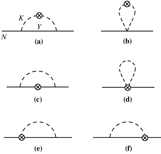
Figure 1: Contributions to the $\bar{s}$ PDF in the nucleon from (a) the kaon rainbow and (b) kaon bubble diagrams, and contributions to the $s$ PDF from (c) the hyperon rainbow, (d) kaon tadpole, and (e), (f) Kroll-Ruderman diagrams. The kaons, $K$, and hyperon, $Y$, are represented by the internal dashed and solid curves, respectively, and the crosses represent insertions of the operators in Eq. (40).

From the operator structures in Eq. (40) we can identify several distinct contributions to the nucleon matrix elements of the strange quark twist-two operators. These are illustrated in Fig. 1, and include the kaon and hyperon rainbow diagrams, the kaon bubble and tadpole contributions, and the Kroll-Ruderman terms that are necessary for the preservation of gauge invariance. Each of these can be expressed in terms of a particular nucleon $\to$ strange hadron splitting function $f_{j}(y)$ and the corresponding PDF in the strange hadron. The moments of the latter can be related to various combinations of coefficients of the hadronic operators in Eq. (40), as we discuss next.

III.3 Matching coefficients and PDF moments

Generally, the coefficients of the operators in Eq. (31) are not constrained by symmetries and must be determined from elsewhere. Within the convolution formalism, Eq. (30), the coefficient $a^{(n)}$ is related, for example, to the $u$-quark or $\bar{s}$-antiquark distribution in the $K^{+}$ meson,

$$\frac{a^{(n)}}{2}=\int_{-1}^{1}dx\,x^{n-1}\,\bar{s}_{K^{+}}(x),$$ (42)

from which we have $a^{(1)}=2$. Within the chiral SU(3) framework, the kaon and pion PDFs are related by $\bar{s}_{K^{+}}=u_{K^{+}}=\bar{s}_{K^{0}}=u_{\pi^{+}}=\bar{d}_{\pi^{+}}=d_{\pi^{-}}=\bar{u}_{\pi^{-}}$ for all $x$ values.

The coefficients $\alpha^{(n)}$, $\beta^{(n)}$ and $\sigma^{(n)}$, on the other hand, are related to the moments of the $u$, $d$ and $s$ PDFs in the bare proton,

$$\frac{5}{6}\alpha^{(n)}+\frac{1}{3}\beta^{(n)}+\sigma^{(n)} = \int_{-1}^{1}dx\,x^{n-1}\,u(x),$$ (43a)

$$\frac{1}{6}\alpha^{(n)}+\frac{2}{3}\beta^{(n)}+\sigma^{(n)} = \int_{-1}^{1}dx\,x^{n-1}\,d(x),$$ (43b)

$$\sigma^{(n)} = \int_{-1}^{1}dx\,x^{n-1}\,s(x).$$ (43c)

Solving Eqs. (43), these coefficients can be obtained in terms of the proton PDFs,

$$\alpha^{(n)} = \int_{-1}^{1}dx\,x^{n-1}\Big{(}\frac{4}{3}u(x)-\frac{2}{3}d(x)-\frac{2}{3}s(x)\Big{)},$$ (44a)

$$\beta^{(n)} = \int_{-1}^{1}dx\,x^{n-1}\Big{(}-\frac{1}{3}u(x)+\frac{5}{3}d(x)-\frac{4}{3}s(x)\Big{)},$$ (44b)

with $\sigma^{(n)}$ given by Eq. (43c). Note that in the SU(3) symmetric limit, the strange quark PDF $s(x)$ in the nucleon is identically zero; for the time being, we keep it explicitly in Eqs. (44) for generality. For $n=1$, the coefficients are then fixed by the conservation of the total charge and strangeness in the nucleon,

$$\alpha^{(1)}=2,\ \ \ \ \beta^{(1)}=1,\ \ \ \ \sigma^{(1)}=0.$$ (45)

To determine the coefficients $\bar{\alpha}^{(n)}$, $\bar{\beta}^{(n)}$ and $\bar{\sigma}^{(n)}$ of the axial vector operators, in contrast, one needs to consider spin-dependent twist-two operators,

$$\mathcal{O}^{\mu_{1}\cdots\mu_{n}}_{\Delta q}=i^{n-1}\bar{q}\gamma_{5}\gamma^{\{\mu_{1}}\overleftrightarrow{D}^{\mu_{2}}\cdots\overleftrightarrow{D}^{\mu_{n}\}}q.$$ (46)

In the effective field theory the spin-dependent twist-two operators can be matched to the hadronic operators according to Shanahan13

$$\mathcal{O}^{\mu_{1}\cdots\mu_{n}}_{\Delta q} = \Big{[}\bar{\alpha}^{(n)}(\overline{\cal B}\gamma^{\mu_{1}}\gamma_{5}{\cal B}\lambda^{q}_{+})+\bar{\beta}^{(n)}(\overline{\cal B}\gamma^{\mu_{1}}\gamma_{5}\lambda^{q}_{+}{\cal B})+\bar{\sigma}^{(n)}(\overline{\cal B}\gamma^{\mu_{1}}\gamma_{5}{\cal B})\,\mathrm{Tr}[\lambda^{q}_{+}]\Big{]}p^{\mu_{2}}\cdots p^{\mu_{n}}$$ (47)

$$+ \Big{[}\alpha^{(n)}(\overline{\cal B}\gamma^{\mu_{1}}{\cal B}\lambda^{q}_{-})+\beta^{(n)}(\overline{\cal B}\gamma^{\mu_{1}}\lambda^{q}_{-}{\cal B})+\sigma^{(n)}(\overline{\cal B}\gamma^{\mu_{1}}{\cal B})\,\mathrm{Tr}[\lambda^{q}_{-}]\Big{]}p^{\mu_{2}}\cdots p^{\mu_{n}}$$

$$+ \mathrm{permutations}\ -\ \mathrm{Tr}.$$

According to the properties of $\mathcal{O}^{\mu_{1}\cdots\mu_{n}}_{q}$ and $\mathcal{O}^{\mu_{1}\cdots\mu_{n}}_{\Delta q}$ under parity transformations Moiseeva:2013 , the coefficients $\{\alpha^{(n)},\beta^{(n)},\sigma^{(n)}\}$ and $\{\bar{\alpha}^{(n)},\bar{\beta}^{(n)},\bar{\sigma}^{(n)}\}$ are the same as for the spin-averaged operators in Eq. (31). Expanding Eq. (47) to lowest order, the coefficients can then be related to the moments of the spin-dependent PDFs in the bare proton by

$$\frac{5}{6}\bar{\alpha}^{(n)}+\frac{1}{3}\bar{\beta}^{(n)}+\bar{\sigma}^{(n)} = \int_{-1}^{1}dx\,x^{n-1}\Delta u(x),$$ (48a)

$$\frac{1}{6}\bar{\alpha}^{(n)}+\frac{2}{3}\bar{\beta}^{(n)}+\bar{\sigma}^{(n)} = \int_{-1}^{1}dx\,x^{n-1}\Delta d(x),$$ (48b)

$$\bar{\sigma}^{(n)} = \int_{-1}^{1}dx\,x^{n-1}\Delta s(x),$$ (48c)

from which the individual coefficients can be determined according to

$$\bar{\alpha}^{(n)} = \int_{-1}^{1}dx\,x^{n-1}\left(\frac{4}{3}\Delta u(x)-\frac{2}{3}\Delta d(x)-\frac{2}{3}\Delta s(x)\right),$$ (49a)

$$\bar{\beta}^{(n)} = \int_{-1}^{1}dx\,x^{n-1}\left(-\frac{1}{3}\Delta u(x)+\frac{5}{3}\Delta d(x)-\frac{4}{3}\Delta s(x)\right).$$ (49b)

As for the spin-averaged PDF in Eqs. (44), here we again keep the bare polarized strange quark PDF $\Delta s(x)$ in the nucleon for generality, even though in the SU(3) limit it is zero. For $n=1$, the coefficients $\bar{\alpha}^{(1)}$ and $\bar{\beta}^{(1)}$ are fixed from the SU(3) decay constants by

$$\bar{\alpha}^{(1)}=\frac{2}{3}(D+3F),\ \ \ \ \bar{\beta}^{(1)}=-\frac{1}{3}(5D-3F).$$ (50)

Along with the nucleon and meson PDFs that appear the calculation of the PDFs in Eq. (30), contributions from PDFs in strange baryons also enter the convolution integrals. Within the chiral SU(3) framework, moments of the strange quark PDFs in the hyperons, $s_{Y}$, are given in terms of the coefficients by

$$\frac{1}{2}\alpha^{(n)}+\sigma^{(n)} = \int_{-1}^{1}dx\,x^{n-1}s_{\Lambda}(x),$$ (51a)

$$\frac{1}{6}\alpha^{(n)}+\frac{2}{3}\beta^{(n)}+\sigma^{(n)} = \int_{-1}^{1}dx\,x^{n-1}s_{\Sigma^{+}}(x)\ =\ \int_{-1}^{1}dx\,x^{n-1}s_{\Sigma^{0}}(x).$$ (51b)

Combining with Eqs. (44), the strange PDFs in the $\Lambda$ and $\Sigma$ hyperons are then related to the $u$ and $d$ PDFs in the proton according to

$$s_{\Lambda}(x) = \frac{1}{3}\Big{[}2u(x)-d(x)+2s(x)\Big{]},$$ (52a)

$$s_{\Sigma^{+}}(x) = s_{\Sigma^{0}}(x)=d(x).$$ (52b)

In practice SU(3) symmetry violating effects Bass10 may give corrections to these relations at the 10%–20% level XWang16 , although a dedicated study of the phenomenological impact on PDFs will be necessary for a more quantitative estimate.

For the strange PDFs associated with the Kroll-Ruderman vertices in Figs. 1(e) and (f), $s^{(\rm KR)}_{Y}(x)$, one makes use of the moment relations

$$\frac{\bar{\alpha}^{(n)}}{\bar{\alpha}^{(1)}} = \int_{-1}^{1}dx\,x^{n-1}s^{(\mathrm{KR})}_{\Lambda}(x),$$ (53a)

$$\frac{\bar{\alpha}^{(n)}+4\bar{\beta}^{(n)}}{\bar{\alpha}^{(1)}+4\bar{\beta}^{(1)}} = \int_{-1}^{1}dx\,x^{n-1}s^{(\mathrm{KR})}_{\Sigma^{+}}(x)\ =\ \int_{-1}^{1}dx\,x^{n-1}s^{(\mathrm{KR})}_{\Sigma^{0}}(x).$$ (53b)

Combining with Eqs. (49), the Kroll-Ruderman strange-quark distributions can then be written in terms of spin-dependent PDFs in the nucleon,

$$s^{(\mathrm{KR})}_{\Lambda}(x) = \frac{1}{D+3F}\,\Big{[}2\Delta u(x)-\Delta d(x)\Big{]},$$ (54a)

$$s^{(\mathrm{KR})}_{\Sigma^{+}}(x) = s^{(\mathrm{KR})}_{\Sigma^{0}}(x)=\frac{1}{F-D}\,\Delta d(x).$$ (54b)

Finally, for the strange quark distributions relevant for the Weinberg-Tomozawa tadpole contribution in Fig. 1(d), $s_{K}^{\rm(tad)}(y)$, one finds the moment relations

$$\frac{1}{12}\left(5\alpha^{(n)}+2\beta^{(n)}\right) = \int_{-1}^{1}dx\,x^{n-1}\,s_{K^{+}}^{\rm(tad)}(x),$$ (55a)

$$\frac{1}{6}\left(\alpha^{(n)}+4\beta^{(n)}\right) = \int_{-1}^{1}dx\,x^{n-1}\,s_{K^{0}}^{\rm(tad)}(x).$$ (55b)

Combining with Eqs. (44), the PDFs associated with the charged and neutral kaon loops are given by

$$s_{K^{+}}^{\rm(tad)}(x) = \frac{1}{2}u(x),$$ (56a)

$$s_{K^{0}}^{\rm(tad)}(x) = d(x).$$ (56b)

These relations provide the complete information on the PDFs in the strange hadrons necessary for the computation of the loop diagrams of Fig. 1. The remaining ingredients needed to evaluate the convolutions in Eq. (30) are the hadronic splitting functions $f_{j}(y)$. In the next section we derive these from the matrix elements of the operators listed in Sec. III.2.

IV Hadronic splitting functions

The hadronic splitting functions $f_{j}(y)$ defined in Eqs. (22) and (23) can be thought of as the effective theory analogs of the quark and gluon splitting functions of perturbative QCD that enter in the PDF evolution equations Altarelli77 . In this case the nucleon $\to$ kaon $+$ hyperon splitting functions are evaluated for each of the hadronic level diagrams in Fig. 1, with the interaction vertices given by the operators in Eqs. (40) and (41). In this section we give the complete set of strange hadron splitting functions in the effective theory. Regularization of the functions will be discussed in Sec. VI. In general we follow the notations introduced for the pion loop corrections in Refs. Z1 ; Burkardt13 ; Salamu15 ; XWang16 , with obvious extensions.

IV.1 Kaon rainbow distribution

We begin with the light-cone distributions associated with the operator insertions on the kaon loop. These give rise to two types of diagrams, illustrated in Fig. 1, involving the kaon rainbow and contact interactions. For the kaon rainbow diagram in Fig. 1(a), the splitting function is given by

$$f_{KY}^{\rm(rbw)}(y) = M\frac{C_{KY}^{2}}{f_{\phi}^{2}}\int\!\frac{d^{4}k}{(2\pi)^{4}}\,\bar{u}(p)(\not{k}\gamma_{5})\frac{i(\not{p}-\not{k}+M_{Y})}{D_{Y}}(\gamma_{5}\not{k})u(p)\frac{i}{D_{K}}\frac{i}{D_{K}}2k^{+}\delta(k^{+}-yp^{+}),$$

where $p$ and $k$ are the physical nucleon and virtual kaon four-momenta, and $D_{K}$ and $D_{Y}$ are the kaon and hyperon virtualities, given by

$$D_{K} = k^{2}-m_{K}^{2}+i\epsilon,$$ (58a)

$$D_{Y} = (p-k)^{2}-M_{Y}^{2}+i\epsilon,$$ (58b)

respectively, with $m_{K}$ and $M_{Y}$ the corresponding kaon and hyperon masses. The spinors $u(p)$ are normalized such that $\bar{u}(p)u(p)=1$. The coefficients $C_{KY}^{2}$ can be obtained from the effective Lagrangian in Eq. (15),

$$C_{K^{+}\Lambda}^{2}=\left(\frac{D+3F}{2\sqrt{3}}\right)^{2},\ \ \ \ \ C_{K^{0}\Sigma^{+}}^{2}=2C_{K^{+}\Sigma^{0}}^{2}=\left(\frac{D-F}{\sqrt{2}}\right)^{2}.$$ (59)

Using the Dirac equation, the integrand in Eq. (IV.1) can be decomposed into several terms,

$$f_{KY}^{\rm(rbw)}(y) = -i\frac{C_{KY}^{2}}{f_{\phi}^{2}}\int\!\frac{d^{4}k}{(2\pi)^{4}}\left[\frac{\overline{M}^{2}(p\cdot k+M\Delta)}{D_{K}^{2}D_{Y}}+\frac{M\overline{M}}{D^{2}_{K}}+\frac{p\cdot k}{D^{2}_{K}}\right]2y\,\delta\left(y-\frac{k^{+}}{p^{+}}\right),$$ (60)

where the sum and difference of the hyperon and nucleon masses are defined as

$$\overline{M} = M_{Y}+M,$$ (61a)

$$\Delta = M_{Y}-M,$$ (61b)

respectively. (Note that $\overline{M}$ and $\Delta$ should both have an index “$Y$” to differentiate between the $\Lambda$ and $\Sigma$ masses; for notational convenience, however, we suppress them in the following.) Using the residue theorem to perform the $k^{-}$ integration and closing the contour in the upper half plane to take the hyperon pole,

$$D_{Y}=(p^{+}-k^{+})\left(p^{-}-k^{-}-\frac{k^{2}_{\perp}+M_{Y}^{2}-i\epsilon}{p^{+}-k^{+}}\right)\ \to\ 0,$$ (62)

one can show that the first term ($\sim 1/D_{K}^{2}D_{Y}$) in the brackets of Eq. (60) corresponds to the on-shell hyperon contribution. This term contributes at $y>0$, and is the contribution usually associated with the “Sullivan process” Sullivan72 ; Signal87 . The second term ($\sim 1/D^{2}_{K}$) in Eq. (60) vanishes after integration by symmetry arguments Burkardt13 . Using the identity Z1

$$\int d^{4}k\frac{2y\,p\cdot k}{D_{K}^{2}}=\int d^{4}k\frac{1}{D_{K}},$$ (63)

the third term in Eq. (60) can be shown to give a singular contribution at $y=0$ Burkardt13 . The splitting function for the kaon rainbow diagram can then be written as a sum of the on-shell and contact ($\delta$-function) contributions,

$$f_{KY}^{(\rm rbw)}(y)=\frac{C_{KY}^{2}\overline{M}^{2}}{(4\pi f_{\phi})^{2}}\left[f_{Y}^{\rm(on)}(y)+f_{K}^{(\delta)}(y)\right].$$ (64)

The on-shell function is given by

$$f_{Y}^{\rm(on)}(y)=y\int\!dk_{\perp}^{2}\,\frac{k_{\perp}^{2}+(My+\Delta)^{2}}{(1-y)^{2}D_{KY}^{2}}F^{\rm(on)},$$ (65)

where

$$D_{KY} = -\left[\frac{k_{\perp}^{2}+yM_{Y}^{2}+(1-y)m_{K}^{2}-y(1-y)M^{2}}{1-y}\right]$$ (66)

is the kaon virtuality for an on-shell hyperon intermediate state. Since the splitting functions for point-particles are ultraviolet divergent, a regularization prescription needs to be used to obtain finite results. Anticipating the discussion of the ultraviolet regularization in Sec. VI below, we introduce in Eq. (65) a function $F^{\rm(on)}$ that regularizes the ultraviolet divergence of the $k_{\perp}^{2}$ integration. The expression in Eq. (65) is identical to the one obtained in the usual Sullivan process with pseudoscalar meson–nucleon–hyperon coupling Signal87 ; Holtmann96 ; Malheiro97 .

The $\delta$-function term $f_{K}^{(\delta)}$ arises from contributions from kaons with zero light-cone momentum ($k^{+}=0$),

$$f_{K}^{(\delta)}(y)=\frac{1}{\overline{M}^{2}}\int\!dk_{\perp}^{2}\,\log\Omega_{K}\,\delta(y)\,F^{(\delta)},$$ (67)

where $\Omega_{K}=k_{\perp}^{2}+m_{K}^{2}$, and $F^{(\delta)}$ is the corresponding regulating function. Note that the numerator in the on-shell function in Eq. (65) depends on the hyperon mass $M_{Y}$ and not on the kaon mass, and hence is labeled by the subscript $Y$. In contrast, the integrand in the $\delta$-function term is independent of the hyperon, and is labeled only by $K$.

IV.2 Kaon bubble distribution

Unlike the pseudoscalar theory, where only the rainbow diagram appears, the pseudovector effective Lagrangian contains the Weinberg-Tomazawa interaction, involving two kaon fields, which give rise to the bubble diagram in Fig. 1(b). For a $K^{+}$ meson loop, the light-cone distribution associated with the bubble graph is given by

$$f^{\rm(bub)}_{K^{+}}(y) = \frac{M}{f_{\phi}^{2}}\int\!\frac{d^{4}k}{(2\pi)^{4}}\,\bar{u}(p)(-i\not{k})u(p)\frac{i}{D_{K}}\frac{i}{D_{K}}2k^{+}\delta(k^{+}-yp^{+}).$$ (68)

Performing the trace over the spinor indices, this can be written as

$$f^{\rm(bub)}_{K^{+}}(y) = \frac{i}{f_{\phi}^{2}}\int\!\frac{d^{4}k}{(2\pi)^{4}}\frac{p\cdot k}{D^{2}_{K}}\,2y\,\delta\left(y-\frac{k^{+}}{p^{+}}\right).$$ (69)

Again using the identity in Eq. (63), the integrand can be expressed in terms of a single kaon propagator, as for the $\delta$-function term in Eq. (67),

$$f_{K^{+}}^{\rm(bub)}(y)=2f_{K^{0}}^{\rm(bub)}(y)=-\frac{\overline{M}^{2}}{(4\pi f_{\phi})^{2}}f_{K}^{(\delta)}(y),$$ (70)

where the relation between the $K^{+}$ and $K^{0}$ contributions is made explicit.

IV.3 Hyperon rainbow distribution

The coupling of the current to the hyperon in the rainbow diagram in Fig. 1(c) leads to the hyperon distribution function given by

$$f_{YK}^{(\rm rbw)}(y) = M\frac{C^{2}_{KY}}{f_{\phi}^{2}}\int\!\frac{d^{4}k}{(2\pi)^{4}}\,\bar{u}(p)(\not{k}\gamma_{5})\frac{i(\not{p}-\not{k}+M_{Y})}{D_{Y}}\,\gamma^{+}\frac{i(\not{p}-\not{k}+M_{Y})}{D_{Y}}(\gamma_{5}\not{k})\,u(p)$$ (71)

$$\hskip 56.9055pt\times\ \frac{i}{D_{K}}\delta(k^{+}-yp^{+}),$$

where one has two hyperon propagators and one kaon propagator. Using the Dirac equation, Eq. (71) can be recast in the reduced form

$$f_{YK}^{(\rm rbw)}(y) = -i\frac{C^{2}_{KY}}{f_{\phi}^{2}}\int\!\frac{d^{4}k}{(2\pi)^{4}}\left[\frac{\overline{M}^{2}(k^{2}-2y\,p\cdot k-2yM\Delta-\Delta^{2})}{D_{K}D_{Y}^{2}}-\frac{2M\overline{M}y+2\overline{M}\Delta}{D_{K}D_{Y}}-\frac{1}{D_{K}}\right]$$ (72)

$$\hskip 56.9055pt\times\ \delta\left(y-\frac{k^{+}}{p^{+}}\right).$$

The first term $(\sim 1/D_{K}D_{Y}^{2})$ in Eq. (72) corresponds to the on-shell hyperon contribution, in analogy with the on-shell term in the kaon rainbow contribution in Eq. (65). The second term $(\sim 1/D_{K}D_{Y})$ arises from the off-shell components of the hyperon propagator, while the third term $(\sim 1/D_{K})$ involves the single kaon propagator and contributes only at $k^{+}=0$. It is convenient therefore to write the total hyperon rainbow distribution function as a sum of three splitting functions associated with the on-shell, off-shell and $\delta$-function contributions,

$$f_{YK}^{(\rm rbw)}(y)=\frac{C_{KY}^{2}\overline{M}^{2}}{(4\pi f_{\phi})^{2}}\left[f_{Y}^{\rm(on)}(y)+f_{Y}^{(\rm off)}(y)-f_{K}^{(\delta)}(y)\right].$$ (73)

The on-shell function $f_{Y}^{\rm(on)}$ is identical to that in Eq. (65), while the $\delta$-function term $f_{K}^{(\delta)}$ is given by Eq. (67). The additional off-shell splitting function in Eq. (73) is given by

$$f_{Y}^{\rm(off)}(y)=\frac{2}{\overline{M}}\int\!dk_{\perp}^{2}\,\frac{My+\Delta}{(1-y)D_{KY}}F^{\rm(off)},$$ (74)

where $F^{\rm(off)}$ is the corresponding off-shell regulating function. As with the on-shell function, the off-shell term also contributes only at $y>0$, and depends only on the hyperon (rather than kaon) mass.

IV.4 Tadpole distribution

The distribution function associated with the tadpole diagram in Fig. 1(d), involving an operator insertion at the $KKpp$ vertex, is given by

$$f_{K^{+}}^{\rm(tad)}(y) = -\frac{M}{f_{\phi}^{2}}\int\!\frac{d^{4}k}{(2\pi)^{4}}\,\bar{u}(p)\gamma^{+}u(p)\frac{i}{D_{K}}\delta(k^{+}-yp^{+}),$$ (75)

for the charged kaon loop, and $f_{K^{0}}^{(\mathrm{tad})}=f_{K^{+}}^{(\mathrm{tad})}/2$ for the neutral kaon loop contribution. Again using the Dirac equation, this can be written in terms of the $f_{K}^{(\delta)}$ function as

$$f_{K^{+}}^{\rm(tad)}(y)=2f_{K^{0}}^{\rm(tad)}(y)=\frac{\overline{M}^{2}}{(4\pi f_{\phi})^{2}}f_{K}^{(\delta)}(y),$$ (76)

so that the tadpole and bubble diagrams are in fact equal and opposite Z1 ,

$$f_{K}^{\rm(tad)}(y)+f_{K}^{\rm(bub)}(y)=0.$$ (77)

IV.5 Kroll-Ruderman distribution

Because of the derivative coupling in the pseudovector theory, by themselves the meson and baryon rainbow diagrams in Figs. 1(a) and (c) are not gauge invariant (the sum of the bubble and tadpole diagrams, on the other hand, is gauge invariant). To ensure gauge invariance of all the chiral loop corrections to the twist-two matrix elements requires, in addition, the Kroll-Ruderman diagrams in Figs. 1(e) and (f). Inserting the relevant $pY$ operators in Eq. (40), the light-cone momentum distribution associated with the Kroll-Ruderman diagrams is given by

$$f^{\rm(KR)}_{YK}(y) = -iM\frac{C^{2}_{KY}}{f_{\phi}^{2}}\int\!\frac{d^{4}k}{(2\pi)^{4}}\,\bar{u}(p)\left[\not{k}\gamma_{5}\frac{i(\not{p}-\not{k}+M_{Y})}{D_{Y}}\gamma^{+}\gamma_{5}+\gamma^{+}\gamma_{5}\frac{i(\not{p}-\not{k}+M_{Y})}{D_{Y}}\not{k}\gamma_{5}\right]u(p)$$ (78)

$$\hskip 56.9055pt\times\ \frac{i}{D_{K}}\delta(k^{+}-yp^{+}).$$

Applying the Dirac equation, the integrand can be decomposed into two terms,

$$f^{\rm(KR)}_{YK}(y) = -2i\overline{M}\frac{C^{2}_{KY}}{f_{\phi}^{2}}\int\!\frac{d^{4}k}{(2\pi)^{4}}\left[\frac{My+\Delta}{D_{K}D_{Y}}+\frac{1}{MD_{K}}\right]\delta\left(y-\frac{k^{+}}{p^{+}}\right).$$ (79)

These can be identified with the off-shell and $\delta$-function contributions from Eqs. (74) and (67), respectively, so that one has

$$f_{YK}^{\rm(KR)}(y) = \frac{C_{KY}^{2}\overline{M}^{2}}{(4\pi f_{\phi})^{2}}\left[-f_{Y}^{\rm(off)}(y)+2f_{K}^{(\delta)}(y)\right].$$ (80)

Comparing the expressions for the kaon and hyperon rainbow diagrams in Eqs. (64) and (73), one finds that the rainbow and KR splitting functions satisfy the identity

$$f_{YK}^{(\rm rbw)}+f_{YK}^{(\rm KR)}=f_{KY}^{(\rm rbw)}.$$ (81)

Together with Eq. (77), this guarantees that the nucleon has zero net strangeness. This will be evident when we consider the convolution expressions for the strange and antistrange PDFs in the nucleon in the next section.

V Strange PDFs in the nucleon: model-independent features

Using the results for the nucleon $\to$ kaon $+$ hyperon splitting functions in Sec. IV, the generic convolution expression in Eq. (30) can be written explicitly for the strange and antistrange PDFs in the nucleon, incorporating the contributions from all of the diagrams shown in Fig. 1. In this section we provide the formulas for the contributions to the $s$ and $\bar{s}$ PDFs in terms of convolution of the rainbow, Kroll-Ruderman, bubble and tadpole splitting functions and the $s$ and $\bar{s}$ PDFs in the strange hadrons derived in Sec. III. Following this we discuss the model-independent chiral nonanalytic behavior of the moments of the $s$ and $\bar{s}$ PDFs, which is required by the chiral symmetry of QCD.

V.1 $s$ and $\bar{s}$ distributions

In the following we will assume for simplicity that the strange and antistrange content of the nucleon arises exclusively through the kaon loops in Fig. 1, and that the bare nucleon is made up entirely of nonstrange quarks. In fact, strictly speaking this constraint is not necessary for the discussion of the $s-\bar{s}$ asymmetry; the only requirement is that any non-chiral contributions (perturbative or nonperbative) are symmetric with respect to $s$ and $\bar{s}$. The $\bar{s}$ PDF in the nucleon can then be written in terms of convolutions of the kaon rainbow and kaon bubble splitting functions from Figs. 1(a) and (b), respectively, with the $\bar{s}$ distribution in the kaon XWang16 ,

$$\bar{s}(x) = \Big{(}\sum_{KY}f_{KY}^{(\rm rbw)}+\sum_{K}f_{K}^{(\rm bub)}\Big{)}\otimes\bar{s}_{K},$$ (82)

where the rainbow terms are summed over $KY=K^{+}\Lambda$, $K^{+}\Sigma^{0}$ and $K^{0}\Sigma^{+}$, and the kaon bubble terms are summed over $K=K^{+}$ and $K^{0}$ for the proton initial state.

For the $s$-quark distribution in the nucleon, on the other hand, the convolution involves the hyperon rainbow, kaon tadpole and Kroll-Ruderman diagrams in Figs. 1(c), (d) and (e)–(f), respectively,

$$s(x) = \sum_{YK}\Big{(}\bar{f}_{YK}^{(\rm rbw)}\otimes s_{Y}+\bar{f}_{YK}^{(\rm KR)}\otimes s_{Y}^{(\rm KR)}\Big{)}+\ \sum_{K}\bar{f}_{K}^{(\rm tad)}\otimes s_{K}^{(\rm tad)},$$ (83)

where the rainbow and Kroll-Ruderman contributions are again summed over all $YK$ combinations, while the tadpole involves a sum over $K^{+}$ and $K^{0}$. For notational convenience, in Eq. (83) we define the functions ${\bar{f}}_{j}(y)\equiv f_{j}(1-y)$. This is necessary since we work in terms of the same momentum fraction $y$ for all kaon and hyperon coupling diagrams in Fig. 1. The strange quark hyperon PDFs, $s_{Y}$, are related to the $u$ and $d$ PDFs in the proton using SU(3) symmetry, as in Eqs. (52), while the Kroll-Ruderman distributions, $s_{Y}^{(\rm KR)}$, are related through SU(3) symmetry to the spin-dependent PDFs in the proton in Eqs. (54). The tadpole distributions, $s_{K}^{(\rm tad)}$, are given in Eqs. (56). Note that with the convention of Eq. (40), the lowest moments of all quark distribution functions in the hadronic states, ${\bar{s}}_{K}$, $s_{Y}$, $s_{Y}^{(\rm KR)}$ and $s_{K}^{(\rm tad)}$, are normalized to unity.

V.2 Leading nonanalytic behavior

A defining feature of the chiral effective theory is the systematic expansion of observables in power series in the meson mass, with generally a priori undetermined coefficients. However, coefficients of terms in the expansion that are not analytic in $m_{K}^{2}$ (such as odd powers of $m_{K}$ or logarithms of $m_{K}$) are independent of the short-distance behavior of the theory and are determined entirely by its infrared properties. Any effective theory or model of QCD must therefore reproduce exactly these coefficients, the most notable of which are the leading nonanalytic (LNA) terms, if it is consistent with the symmetries of QCD. For moments of PDFs, the LNA terms were found previously TMS00 ; Chen02 ; Arndt01 to have a characteristic $m_{\pi}^{2}\log m_{\pi}^{2}$ dependence (for pion loops), a feature which was applied Detmold01 to analyze the chiral behavior of lattice moments of the isovector quark PDFs.

In the present formulation, we can derive the LNA behavior of the $n$-th moments of the individual $s$ and $\bar{s}$ PDFs, defined as

$$S^{(n-1)} = \int_{0}^{1}dx\,x^{n-1}\,s(x),$$ (84a)

$$\overline{S}^{(n-1)} = \int_{0}^{1}dx\,x^{n-1}\,\bar{s}(x),$$ (84b)

and hence those of the $s-\bar{s}$ asymmetry, from the convolution formulas (82) and (83) and the nonanalytic properties of the splitting functions. Of greatest phenomenological interest will be the $n=1$ and $n=2$ moments of the PDFs, which correspond to the number and momentum sum rules. The LNA behavior of the PDF moments is determined by the LNA behavior of the moments of the splitting functions, each of which can be expressed in terms of the three basic functions $f_{Y}^{\rm(on)}$, $f_{Y}^{\rm(off)}$ and $f_{K}^{(\delta)}$ derived in Sec. IV. We define the $n$-th moments of these, integrated over the physical $y$ range, as

$${\tilde{f}}_{{\rm on},Y}^{(n)} = \int_{0}^{1}dy\,y^{n-1}\,f_{Y}^{(\rm on)}(y),$$ (85a)

$${\tilde{f}}_{{\rm off},Y}^{(n)} = \int_{0}^{1}dy\,y^{n-1}\,f_{Y}^{(\rm off)}(y),$$ (85b)

$${\tilde{f}}_{\delta,K}^{(n)} = \int_{0}^{1}dy\,y^{n-1}\,f_{K}^{(\delta)}(y).$$ (85c)

The LNA behavior is intrinsically infrared and is obtained by considering the lower bound of the $k_{\perp}$ integration, in each of the splitting functions. Expanding in powers $m_{K}/M$ and $\Delta/M$, we find for the $n=1$ moments,

$$\overline{M}^{2}{\tilde{f}}_{{\rm on},Y}^{(1)}\Big{|}_{\rm LNA} = (4m_{K}^{2}-6\Delta^{2})\log m_{K}^{2}+6R\,\Delta\,\log\frac{\Delta-R}{\Delta+R},$$ (86a)

$$\overline{M}^{2}{\tilde{f}}_{{\rm off},Y}^{(1)}\Big{|}_{\rm LNA} = -2m_{K}^{2}\log m_{K}^{2}-\frac{2R^{3}}{M_{Y}}\log\frac{\Delta-R}{\Delta+R},$$ (86b)

$$\overline{M}^{2}{\tilde{f}}_{\delta,K}^{(1)}\Big{|}_{\rm LNA} = -m_{K}^{2}\log m_{K}^{2},$$ (86c)

where $R=\sqrt{\Delta^{2}-m_{K}^{2}}$ and ${\cal O}(m_{K}/M,\Delta/M)$ corrections have been neglected. For the $n=2$ moments of the splitting functions, we find the LNA behavior

$$\overline{M}^{2}{\tilde{f}}_{{\rm on},Y}^{(2)}\Big{|}_{\rm LNA} = \frac{4\Delta}{3M_{Y}}(-6m_{K}^{2}+7\Delta^{2})\log m_{K}^{2}+\frac{2R}{3M_{Y}}(5m_{K}^{2}-14\Delta^{2})\,\log\frac{\Delta-R}{\Delta+R},$$ (87a)

$$\overline{M}^{2}{\tilde{f}}_{{\rm off},Y}^{(2)}\Big{|}_{\rm LNA} = \frac{2\Delta}{3M_{Y}}(3m_{K}^{2}-2\Delta^{2})\log m_{K}^{2}-\frac{4R^{3}}{3M_{Y}}\log\frac{\Delta-R}{\Delta+R},$$ (87b)

$$\overline{M}^{2}{\tilde{f}}_{\delta,K}^{(2)}\Big{|}_{\rm LNA} = 0.$$ (87c)

Note that because the function $f_{K}^{(\delta)}(y)\propto\delta(y)$, its $n=2$ and all higher moments vanish.

The LNA behavior of the $n$-th moments of the $\bar{s}$ PDF is then given by

$$\overline{S}^{(n-1)}_{\rm LNA} = \frac{\overline{M}^{2}}{(4\pi f_{\phi})^{2}}\sum_{KY}\Big{[}C_{KY}^{2}\,{\tilde{f}}_{{\rm on},Y}^{(n)}+\left(C_{KY}^{2}-1\right){\tilde{f}}_{\delta,K}^{(n)}\Big{]}_{\rm LNA}\,\overline{S}^{(n-1)}_{K},$$ (88)

where $\overline{S}^{(n-1)}_{K}$ are the moments of the $\bar{s}$ PDF in the kaon, and the sums are taken over the appropriate hyperons and kaons.

For the strange-quark PDF in the nucleon, because the convolutions in Eq. (83) involve the splitting functions evaluated at $(1-y)$, the expressions for the moments involve binomial sums over the moments. Specifically, one has

$$S^{(n-1)}_{\rm LNA} = \frac{\overline{M}^{2}}{(4\pi f_{\phi})^{2}}\sum_{KY}\sum_{k=1}^{n}\binom{n-1}{k-1}(-1)^{k-1}$$

$$\times\left\{C_{KY}^{2}\,\Big{[}{\tilde{f}}_{{\rm on},Y}^{(k)}+{\tilde{f}}_{{\rm off},Y}^{(k)}-{\tilde{f}}_{\delta,K}^{(k)}\Big{]}_{\rm LNA}S^{(n-1)}_{Y}+\ C_{KY}^{2}\,\Big{[}2{\tilde{f}}_{\delta,K}^{(k)}-{\tilde{f}}_{{\rm off},Y}^{(k)}\Big{]}_{\rm LNA}S^{(n-1)}_{\rm(KR)Y}-\ \Big{[}{\tilde{f}}_{\delta,K}^{(k)}\Big{]}_{\rm LNA}S^{(n-1)}_{\rm(tad)Y}\right\}.$$

The expressions in Eqs. (88) and (LABEL:eq:sLNA) hold for any $n$, including $n=1$ and 2. In particular, from Eqs. (42), (45) and (50) each of the $n=1$ moments of the PDFs in the strange hadrons is normalized to unity. The LNA contributions to the $n=1$ moments for the strange and antistrange distributions in the proton are therefore equivalent,

$$S^{(0)}_{\rm LNA}\ = \frac{\overline{M}^{2}}{(4\pi f_{\phi})^{2}}\sum_{KY}\Big{[}C_{KY}^{2}\,{\tilde{f}}_{{\rm on},Y}^{(1)}+\left(C_{KY}^{2}-1\right){\tilde{f}}_{\delta,K}^{(1)}\Big{]}_{\rm LNA}\ =\ \overline{S}^{(0)}_{\rm LNA},$$ (90)

as required by strangeness conservation. This is no longer the case for $n=2$ and higher moments, for which the various moments in the strange hadrons $S^{(n-1)}_{j}$ are no longer related. Furthermore, for $n=2$ the antistrange quark moment $\overline{S}^{(1)}$ depends on ${\tilde{f}}_{j}^{(2)}$, while the strange quark moment $S^{(1)}$ depends on the combination ${\tilde{f}}_{j}^{(1)}-{\tilde{f}}_{j}^{(2)}$ from the combinatorics in Eq. (LABEL:eq:sLNA).

VI Regularization

For point particles, the functions $F^{\rm(on)}$, $F^{\rm(off)}$ and $F^{(\delta)}$ for the on-shell, off-shell and $\delta$-function distributions in Eqs. (65), (67) and (74), respectively, are each set to unity, and the integrations over the kaon loop momenta $k$ are ultraviolet divergent. In the effective theory for the hadrons, which in nature always have finite size, some regularization prescription must be adopted to render the integrals finite. In practice this is achieved by the regulating functions aquiring momentum dependence such that the contributions from large momenta are suppressed.

In the literature various prescriptions have been adopted, ranging from dimensional regularization in traditional chiral perturbation theory chiPT to sharp cutoffs in $k_{\perp}$ Salamu15 or form factors in more phenomenological approaches Speth98 . Regularization with the help of a finite-range regulator has been advocated Donoghue99 ; Wright00 ; Thomas03 as a practical method which reflects the finite size of the baryon to which the chiral field couples. The effectiveness of the various prescriptions in providing accurate results for expansions of various static properties of hadrons away from the chiral regime have been discussed in Refs. FRR1 ; FRR2 .

In any chosen regularization scheme it is important to respect the symmetries of the underlying hadronic field theory, including Lorentz invariance, gauge invariance, and chiral symmetry. Schemes such as dimensional regularization and PV regularization are known to preserve both chiral and Lorentz symmetries, while for other prescriptions some of these symmetries are not satisfied. Simple application of hadronic form factors, for example, can lead to problems with gauge invariance Z1 ; Faessler03 , and (in the present application) with strangeness conservation in the nucleon. Restoration of gauge invariance in the presence of form factors requires the generalization of the chiral Lagrangian to include nonlocal terms Faessler03 ; Terning91 ; Nonlocal16 . Following the approach adopted in Ref. XWang16 , here we utilize the PV regularization method, which offers many of the advantages of finite range regularization and preserves all of the required symmetries.

VI.1 Pauli-Villars regularization

The PV regularization scheme involves subtracting from the point-like amplitudes expressions in which the propagator mass is replaced by a cutoff mass $\mu_{1}$, such that in the ultraviolet limit the differences between the amplitudes vanish. For the on-shell distribution $f_{Y}^{(\rm on)}(y)$, for example, one replaces the $1/D_{KY}^{2}$ propagator in Eq. (65) by $1/D_{KY}^{2}-1/D_{\mu_{1}}^{2}$, where $D_{\mu_{1}}=k^{2}-\mu_{1}^{2}$. This is equivalent to setting the regulating function $F^{\rm(on)}$ in Eq. (65) to

$$F^{\rm(on)}=1-\frac{D_{KY}^{2}}{D_{\mu_{1}}^{2}}.$$ (91)

Similarly for the off-shell hyperon function $f_{Y}^{(\rm off)}(y)$, one replaces the propagator $1/D_{KY}$ in Eq. (74) by $1/D_{KY}-1/D_{\mu_{1}}$, in which case the off-shell regulating function $F^{\rm(off)}$ is given by

$$F^{\rm(off)}=1-\frac{D_{KY}}{D_{\mu_{1}}}.$$ (92)

For the $\delta$-function term $f_{K}^{(\delta)}(y)$, on the other hand, because both the $k^{-}$ and $k_{\perp}^{2}$ integrations are individually ultraviolet divergent, a single PV subtraction is not sufficient, and two subtractions are necessary in the kaon propagator to render the integrals finite,

$$\frac{1}{D_{K}}\to\frac{1}{D_{K}}-\frac{a_{1}}{D_{\mu_{1}}}-\frac{a_{2}}{D_{\mu_{2}}}.$$ (93)

Here the two subtraction constants $a_{1}$ and $a_{2}$ are related to the cutoff masses $\mu_{1}$ and $\mu_{2}$ by

$$a_{1}=\frac{\mu_{2}^{2}-m_{K}^{2}}{\mu_{2}^{2}-\mu_{1}^{2}},\ \ \ \ \ a_{2}=\frac{\mu_{1}^{2}-m_{K}^{2}}{\mu_{1}^{2}-\mu_{2}^{2}},$$ (94)

so that in the $k\to\infty$ limit the propagator term behaves as $\sim 1/k^{6}$. This leads to an effective regularizing function in Eq. (67) given by

$$F^{(\delta)}=1-\frac{a_{1}\log\Omega_{\mu_{1}}+a_{2}\log\Omega_{\mu_{2}}}{\log\Omega_{K}},$$ (95)

with $\Omega_{\mu_{i}}=k_{\perp}^{2}+\mu_{i}^{2}$. The free parameters in the calculation are then the two cutoffs $\mu_{1}$ and $\mu_{2}$, the constraints on which we discuss in the following.

VI.2 Constraints on cutoff parameters

Since the on-shell function, $f_{Y}^{(\rm on)}(y)$, depends only on the $\mu_{1}$ cutoff parameter, the natural process to consider for constraining $\mu_{1}$ phenomenologically is the inclusive production of $\Lambda$ hyperons in $pp$ collisions. For large values of the produced $\Lambda$ momentum ($1-y\gtrsim 0.7$) and small $k_{\perp}\lesssim 100$ MeV, the dominant contribution to the production process is expected to be from the exchange of a single $K^{+}$ meson. At larger kaon momenta $y$ (smaller $1-y$) multiple meson exchanges and contributions from heavier meson and baryon intermediate states will become more important Holtmann96 ; Kopeliovich12 . These, however, cannot be computed within the chiral effective theory framework and will not be considered here.

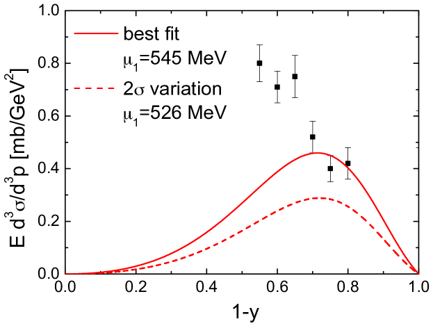
Figure 2: Differential cross section for inclusive $\Lambda$ production in $pp$ scattering as a function of the momentum fraction $1-y$ carried by the hyperon, for $k_{\perp}=75$ MeV Blobel78 . The curves are fitted to the data at $1-y>0.7$, with the best fit (solid line) obtained with the mass parameter $\mu_{1}=545$ MeV, and the fit $2\sigma$ below the central values (dashed line) with $\mu_{1}=526$ MeV.

The differential cross section for the $pp\to\Lambda X$ reaction with $K^{+}$ exchange is given by Holtmann96

$$E\frac{d^{3}\sigma}{d^{3}p} = \frac{C_{K^{+}\Lambda}^{2}\overline{M}^{2}}{16\pi^{3}f_{\phi}^{2}}\frac{y\left[k_{\perp}^{2}+(My+\Delta)^{2}\right]}{(1-y)D_{K^{+}\Lambda}^{2}}F^{\rm(on)}(y,k_{\perp}^{2})\,\sigma^{pK^{+}}_{\rm tot}(sy),$$ (96)

where $s$ is the $pp$ center of mass energy squared, and the total $pK^{+}$ cross section $\sigma^{pK^{+}}_{\rm tot}$ is evaluated at the $pK^{+}$ squared center of mass energy $sy$. In Fig. 2 the inclusive $\Lambda$ production cross section data from Ref. Blobel78 are shown as a function of the hyperon momentum fraction $1-y$, for $k_{\perp}=75$ MeV. Taking the standard, constant value $\sigma^{pK^{+}}_{\rm tot}=(19.9\pm 0.1)$ mb Povh92 for the total $pK^{+}$ cross section in Eq. (96), we fit the $\mu_{1}$ parameter in the calculated cross section to the data at small $y$ that are dominated by the lightest, kaon-exchange contribution. The best fit to data at $y<0.3$ is obtained for the value $\mu_{1}=(0.545\pm 0.009)$ GeV, where the error is statistical, giving a $\chi^{2}_{\rm dof}=1.06$. Extending the fitted range to $y<0.4$ gives a significantly worse fit, with $\chi^{2}_{\rm dof}\approx 3.7$, suggesting the presence of other, non-kaonic contributions already for $y\gtrsim 0.3$, consistent with the findings of previous model-dependent analyses Holtmann96 ; Kopeliovich12 . Including additional terms from non-kaonic backgrounds would in practice reduce the magnitude of the kaon contributions allowed by the data, so that the above cutoff can be taken as an upper limit. As an estimate of the systematic uncertainty in this procedure, we also consider a fit that lies two standard deviations below the best fit, for which the cutoff parameter is $\mu_{1}=526$ MeV.

Additional constraints on the $\mu_{1}$ parameter can in principle be obtained from comparisons of the $\bar{s}$ PDF in Eq. (82) calculated from kaon loops with the phenomenological $\bar{s}$ distribution extracted from global PDF fits. The availability of antineutrino DIS data CCFR ; NuTeV , for example, can isolate the $\bar{s}$ distribution from the $s$-quark PDF, which contributes through the absorption of a $W^{+}$ boson in neutrino DIS. In practice, however, the uncertainties on the $\nu/\bar{\nu}$ data are typically considerably larger than those on the corresponding electromagnetic cross sections. Furthermore, the neutrino measurements are usually performed on nuclear targets, so that the cross sections must be corrected for nuclear effects, which are not completely understood for neutrino scattering. Thus, in practice little direct information exists on the $\bar{s}$ PDF from global analyses, which in fact usually assume symmetric $s$ and $\bar{s}$ distributions.

On the other hand, the $s$-quark PDF is sensitive to the $\mu_{2}$ parameter in the $F^{(\delta)}$ function that regulates the kaon tadpole contribution in Eq. (83). Even though the splitting function associated with the tadpole loop is a $\delta$-function at the kaon momentum fraction $y=0$, Eq. (76), the fact that the convolution (83) involves a coupling at the hyperon vertex means that this contribution to $s(x)$ in the nucleon will be proportional to $s_{K}^{(\rm tad)}(x)$. Using the SU(3) relations in Eq. (56), this term will then produce a valence-like shape that is nonzero at $x>0$. Comparisons with the phenomenological $s$-quark PDF as a function of $x$ can then constrain the value of the $\mu_{2}$ parameter.

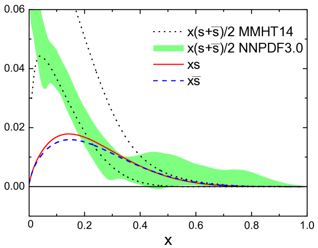
Figure 3: Strange quark $xs$ (solid red curve) and antiquark $x\bar{s}$ (dashed blue curve) PDFs from kaon loops for the best fit parameters $\mu_{1}=545$ MeV and $\mu_{2}=600$ MeV, compared with the phenomenological $x(s+\bar{s})/2$ distribution from the MMHT14 MMHT14 (black dotted curves) and NNPDF3.0 NNPDF3.0 (green shaded band) global analyses at $Q^{2}=1$ GeV².

In Fig. 3 the combined $s+\bar{s}$ distribution from kaon loops is compared with several recent parametrizations from global PDF analyses MMHT14 ; NNPDF3.0 . In the evaluation of the $\bar{s}$ PDF in Eq. (82), at the lowest order to which we work the strange quark PDF in the kaon is related by SU(3) symmetry to the valence PDF in the pion, $\bar{s}_{K^{+}}=\bar{s}_{K^{0}}=\bar{d}_{\pi^{+}}$, with the latter taken from a global PDF fit to $\pi N$ Drell-Yan data by Aicher et al. Aicher10 . For the strange quark PDFs in the hyperons, $s_{Y}$, and the strange tadpole distributions, $s_{K}^{(\rm tad)}$, the SU(3) constraints in Eqs. (52) and (56), respectively, are used to relate these to the $u$ and $d$ PDFs in the proton, for which the parametrization by Martin et al. MRST98 is utilized. For the strange KR distributions $s_{Y}^{(\rm KR)}$ at the $NKY$ vertex, on the other hand, Eqs. (54) are used to express these in terms of the spin-dependent PDFs in the nucleon, and in practice we take the fit from Ref. LSS10 for both the polarized PDFs and the $D$ and $F$ values. The results using other parametrizations for the spin-averaged MMHT14 ; NNPDF3.0 ; CJ15 or spin-dependent DSSV09 ; JAM15 $u$ and $d$ distributions yields very similar results.

The comparison of the $s$ and $\bar{s}$ PDFs in Fig. 3 calculated from kaon loops uses the maximum value of $\mu_{1}$ allowed by the $pp\to\Lambda X$ data in Fig. 2, and adjusts the maximum value of $\mu_{2}$ to ensure that the sum $x(s+\bar{s})$ does not exceed the phenomenological parametrization at $Q^{2}=1$ GeV² within the quoted uncertainties, $(s+\bar{s})_{\rm loops}\leq(s+\bar{s})_{\rm tot}$. Interestingly, while the MMHT14 parametrization MMHT14 allows a slightly larger $s+\bar{s}$ at $x\lesssim 0.3$, it places stronger constraints at larger $x$ values. On the other hand, the NNPDF3.0 analysis, which uses a somewhat different fitting methodology, gives slightly smaller strange PDFs at low $x$, but permits a larger magnitude for $s+\bar{s}$ at $x\gtrsim 0.4$. Taken as an approximately representative sample of the current uncertainty on the strange quark PDF, the combined phenomenological constraints in Fig. 3 allow a maximum value for the $\mu_{2}$ parameter of 600 MeV. If we were to take the lower $\mu_{1}$ value from the inclusive $\Lambda$ production data in Fig. 2, $\mu_{1}=526$ MeV, corresponding to the 2$\sigma$ deviation, the loop contributions to $s+\bar{s}$ would remain consistent with the phenomenological PDF constraints for $\mu_{2}$ as large as 894 MeV.

VII Strange asymmetry in the nucleon

Having obtained contraints on the $\mu_{1}$ and $\mu_{2}$ parameters in our calculated $s$ and $\bar{s}$ PDFs from existing data on inclusive $\Lambda$ production in $pp$ scattering and from phenomenological PDFs, in this section we discuss in more detail the implications of our results for the strange asymmetry in the nucleon both as a function of $x$ and for the lowest moments. We consider the two extremal cases for the cutoff parameters, with the maximal $\mu_{1}$ from the $pp$ data combined with the maximum $\mu_{2}$ from the comparison with the $s+\bar{s}$ PDFs, $(\mu_{1},\mu_{2})=(545,600)$ MeV, and with a lower $\mu_{1}$ value for the 2$\sigma$ fit of the $\Lambda$ production data and a correpondingly higher $\mu_{2}$ value, $(\mu_{1},\mu_{2})=(526,894)$ MeV. This range will provide a reasonable estimate of the systematic uncertainty in our calculation.

To illustrate the variation for this range of cutoffs of the $KY$ splitting functions, in Fig. 4 we plot the on-shell and off-shell functions $f_{\Lambda}^{\rm(on)}$ and $f_{\Lambda}^{\rm(off)}$ in Eqs. (65) and (74) for the $p\to K^{+}\Lambda$ dissociation as a function of $y$. The on-shell distributions have a characteristic shape that peaks around $y\approx 0.3-0.4$, with an obviously larger magnitude for the higher cutoff, $\mu_{1}=545$ MeV. Interestingly, the off-shell function is negative, with its magnitude peaking at $y\approx 0.2$, and remains nonzero at $y=0$. The latter result can be understood from the integrand of the $f_{Y}^{\rm(off)}$ function in Eq. (74): whereas for the on-shell function in Eq. (65) the $k_{\perp}$ dependence is multiplied by an overall factor $y$, for the off-shell function the term in (74) proportional to $\Delta$ remains finite in the $y\to 0$ limit.

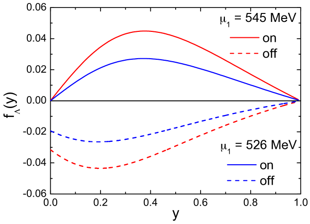
Figure 4: On-shell (solid lines) and off-shell (dashed lines) contributions to the proton $\to K^{+}\Lambda$ splitting functions for $\mu_{1}=545$ MeV (red curves) and $\mu_{1}=526$ MeV (blue curves).

Note that the shape of the on-shell function in Fig. (4), with the PV regulator, is qualitatively similar to the splitting functions found in the literature which have been computed in terms of form factors at the $NKY$ vertex Speth98 . A comparison of the $f_{\Lambda}^{\rm(on)}$ splitting functions computed with PV regularization with the results obtained using $t$-dependent Thomas83 ; Kumano91 ; MTS91 ; MST94 ; Kumano98 or $s$-dependent Holtmann96 ; Malheiro97 ; Zoller92 ; MT93 form factors for the function $F^{\rm(on)}$ is shown in Fig. 5. For the $t$-dependent form, the commonly used monopole shape is taken, so that the function $F^{\rm(on)}$, which is the square of the form factor, is a dipole,

$$F^{\rm(on)} = \left(\frac{\Lambda_{t}^{2}-m_{K}^{2}}{\Lambda_{t}^{2}-t}\right)^{2},$$ (97)

where $t\equiv k^{2}=-[k_{\perp}^{2}+y(M_{Y}^{2}-(1-y)M^{2})]/(1-y)$. For the $s$-dependent form, an exponential shape is used,

$$F^{\rm(on)} = \exp\left(\frac{M^{2}-s}{\Lambda_{s}^{2}}\right),$$ (98)

where $s\equiv(m_{K}^{2}+k_{\perp}^{2})/y+(M_{Y}^{2}+k_{\perp}^{2})/(1-y)$. The normaliation of each of the splitting functions is fixed to be the same value as the PV-regulated form with cutoff mass $\mu_{1}=0.545$ GeV, which is achieved with $t$-dependent monopole cutoff mass parameter $\Lambda_{t}=0.928$ GeV and $s$-dependent exponential mass $\Lambda_{s}=1.293$ GeV.

The shape with the PV regulator is slightly harder compared with the other forms, but is closer to the $t$-dependent monopole at low values of $y$. Because of the $1/y$ and $1/(1-y)$ exponential suppression in the $s$-dependent form factor, the result using Eq. (98) is significantly damped as $y\to 0$ and $y\to 1$.

The $s$-dependent form in particular has been inspired in the literature by attempts to satisfy $y\leftrightarrow 1-y$ symmetry relations between the splitting functions for the kaon rainbow [Fig. 1(a)] and hyperon rainbow [Fig. 1(c)] diagrams Zoller92 ; Holtmann96 . Namely, because of the kinematic relation $s+t+u=M^{2}+m_{K}^{2}+M_{Y}^{2}$, where $u\equiv(p-k)^{2}$, form factors that are functions of $s$ automatically satisfy the $t$- and $u$-channel crossing symmetry. On the other hand, the $s$-dependent form is generally not Lorentz invariant (it is invariant only under the light-cone longitudinal and transverse boosts). Furthermore, the use of momentum dependent form factors, whether funtions of $t$ or $s$, is known to lead to a violation of gauge invariance, requiring specific prescriptions to restore the gauge symmetry through the introduction of nonlocal terms Faessler03 ; Terning91 ; Nonlocal16 . Calculations of PDFs using the splitting functions computed with form factors on the basis of the local interactions in Fig. 1, let alone the rainbow diagrams by themselves, are therefore in general not invariant under gauge or chiral transformations.

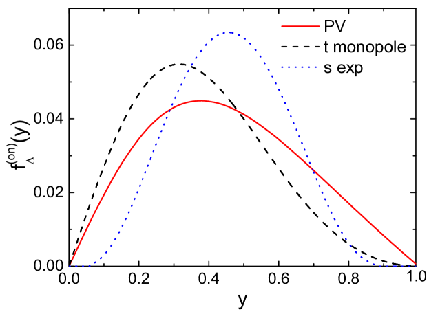
Figure 5: Comparison of the on-shell proton $\to K^{+}\Lambda$ splitting function for the PV regulator with $\mu_{1}=545$ MeV (red solid curve) with the function computed with a $t$-dependent monopole form factor for $\Lambda_{t}=0.928$ GeV (black dashed curve) and with an $s$-dependent form factor for $\Lambda_{s}=1.293$ GeV (blue dotted curve), normalized to give the same value when integrated over $y$.

It is instructive to quantify the relative contributions to the strange-quark PDFs, as well as to their moments, arising from the various diagrams in Fig. 1. As illustrated above in Fig. 3, the respective magnitudes and shapes of the total contributions to $s$ and $\bar{s}$ at $x>0$ are similar, with $s$ slightly larger than $\bar{s}$ at the peak around $x\approx 0.15$. While only the on-shell piece contributes to $\bar{s}$ at $x>0$ [Eq. (82)], there are 3 contributions to the $s$-quark PDF at nonzero $x$ [Eq. (83)],

$$s(x) = \big{(}s^{\rm(on)}+s^{\rm(off)}+s^{(\delta)}\big{)}_{\rm rbw}\ +\ s^{(\delta)}_{\rm tad}\ +\ \big{(}s^{\rm(off)}+s^{(\delta)}\big{)}_{\rm KR}$$ (99)

$$= \underbrace{s^{\rm(on)}_{\rm rbw}}_{\rm on-shell}\ +\ \underbrace{s^{\rm(off)}_{\rm rbw}+s^{\rm(off)}_{\rm KR}}_{\rm off-shell}\ +\ \underbrace{s^{(\delta)}_{\rm rbw}+s^{(\delta)}_{\rm tad}+s^{(\delta)}_{\rm KR}}_{\rm\delta-function}\,,$$

$$\bar{s}(x) = \big{(}\bar{s}^{\rm(on)}+\bar{s}^{(\delta)}\big{)}_{\rm rbw}\ +\ \bar{s}^{(\delta)}_{\rm bub}$$ (100)

$$= \underbrace{\bar{s}^{\rm(on)}_{\rm rbw}}_{\rm on-shell}+\ \underbrace{\bar{s}^{(\delta)}_{\rm rbw}+\bar{s}^{(\delta)}_{\rm bub}}_{\rm\delta-function}\,,$$

where we have suppressed the $x$ dependence in each of the terms on the right-hand-side. For the best fit parameters $(\mu_{1},\mu_{2})=(545,600)$ MeV (top panels in Fig. 6), the KR diagrams in Figs. 1(e)–(f) give the largest overall contribution to $s(x)$, with the rainbow and tadpole contributions relatively small. Closer inspection of the various diagrams shows large cancellations between the off-shell terms in the rainbow and KR diagrams, and between the $\delta$-function terms arising from the rainbow, KR and tadpole diagrams. The net effect is that the total $s$-quark distribution is well approximated by the on-shell part of the rainbow diagram, with the total off-shell and $\delta$-function terms being relatively small. This illustrates the vital role played by the tadpole and KR diagrams, which are needed in a consistent theory along with the rainbow contributions. It also explains the phenomenological success of earlier calculations of meson loop corrections to PDFs in terms of on-shell rainbow contributions only.

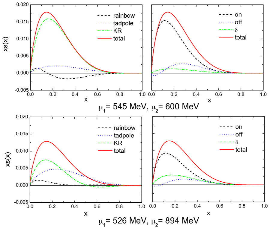
Figure 6: Contributions to the $xs$ distribution at $Q^{2}=1$ GeV² from various kaon loop diagrams in Fig. 1, for $(\mu_{1},\mu_{2})=(545,600)$ MeV (top panels) and $(\mu_{1},\mu_{2})=(526,894)$ MeV (bottom panels). The decomposition of the total into rainbow, tadpole and KR contributions (left panels) is contrasted with the decomposition into on-shell, off-shell and $\delta$-function contributions (right panels), according to Eqs. (99)–(100).

For the alternative fit parameters from Sec. VI, namely $(\mu_{1},\mu_{2})=(526,894)$ MeV (bottom panels in Fig. 6), the magnitude of the total strange-quark PDF is slightly smaller, and the cancellations between the various off-shell and $\delta$-function terms are not as dramatic. Nevertheless, even though the on-shell part of the rainbow diagram does not saturate the total contribution as completely, a similar qualitative behavior is observed here also.

Table 1: Individual contributions to the first ($n=1$) moments $S^{(0)}$ and $\overline{S}^{(0)}$ of the $s$ and $\bar{s}$ PDFs from the diagrams in Fig. 1 at $Q^{2}=1$ GeV² for the two extreme cases considered, $(\mu_{1},\mu_{2})=(545,600)$ MeV and (526, 894) MeV. The moments are given in units of $10^{-2}$.

$(\mu_{1},\mu_{2})$	(545, 600) MeV		(526, 894) MeV
	$S^{(0)}$	$\overline{S}^{(0)}$	$S^{(0)}$	$\overline{S}^{(0)}$
rbw (on)	4.91	4.91	2.97	2.97
rbw (off)	$-4.86$	—	$-2.93$	—
rbw ($\delta$)	0.20	$-0.20$	0.47	$-0.47$
tad ($\delta$)	0.59	—	1.36	—
bub ($\delta$)	—	0.59	—	1.36
KR off)	4.86	—	2.93	—
KR ($\delta$)	$-0.40$	—	$-0.94$	—
Total	5.30	5.30	3.86	3.86

Table 2: Contributions to the second ($n=2$) moments $S^{(1)}$ and $\overline{S}^{(1)}$ of the $s$ and $\bar{s}$ PDFs from kaon loops at $Q^{2}=1$ GeV² for the two extreme cases considered, $(\mu_{1},\mu_{2})=(545,600)$ MeV and (526, 894) MeV. The moments are given in units of $10^{-3}$.

$(\mu_{1},\mu_{2})$	(545, 600) MeV		(526, 894) MeV
	$S^{(1)}$	$\overline{S}^{(1)}$	$S^{(1)}$	$\overline{S}^{(1)}$
rbw (on)	4.67	5.68	2.83	3.41
rbw (off)	$-5.41$	—	$-3.28$	—
rbw ($\delta$)	0.34	0	0.79	0
tad ($\delta$)	0.95	—	2.21	—
bub ($\delta$)	—	0	—	0
KR (off)	6.35	—	3.85	—
KR ($\delta$)	$-0.81$	—	$-1.87$	—
Total	6.10	5.68	4.53	3.41

More quantitatively, the contributions of the various terms to the moments of the $s$ and $\bar{s}$ PDFs are listed in Tables 2 and 2 for the $S^{(0)}$, $\overline{S}^{(0)}$ and $S^{(1)}$, $\overline{S}^{(1)}$ moments, respectively. For the lowest ($n=1$) moments, the off-shell parts of the rainbow and KR contributions to $S^{(0)}$ in fact cancel exactly, leaving the on-shell component as the dominant term, and the remaining contributions distributed among the $\delta$-function pieces. Strangeness conservation requires the on-shell contribution to $\overline{S}^{(0)}$ to be identical to that for $S^{(0)}$, with equivalent contributions from the tadpole and bubble diagrams to the strange and antistrange moments, respectively.

For the second ($n=2$) moments in Table 2, similarly large cancellations are observed between the off-shell contributions to the $S^{(1)}$ moment from the rainbow and KR diagrams. Cancellations also occur between the positive $\delta$-function parts of the rainbow and tadpole diagrams with the negative $\delta$-function component of the KR diagrams. In contrast, because of the additional power of $x$ in the $n=2$ moment definition, only the on-shell part of rainbow diagram contributes to the $\bar{s}$ moment. The net effect is thus a positive difference $S^{-}\equiv S^{(1)}-\overline{S}^{(1)}$. Note that while for the larger $\mu_{1}$ cutoff value both the $S^{(1)}$ and $\overline{S}^{(1)}$ moments are bigger, the difference $S^{-}=0.42\times 10^{-3}$ for $\mu_{1}=545$ MeV at $Q^{2}=1$ GeV² is smaller than for the lower cutoff $\mu_{1}=526$ MeV, for which $S^{-}=1.12\times 10^{-3}$, as is also apparent in Fig. 7. Here both the sum $x(s+\bar{s})$ and difference $x(s-\bar{s})$ are illustrated at $Q^{2}=1$ GeV² for both sets of cutoff values. To display the sum and difference on the same plot, we scale the much larger $x(s+\bar{s})$ distribution by a factor 1/4.

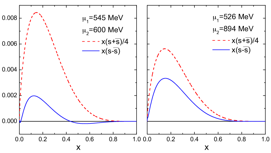
Figure 7: Total sum $x(s+\bar{s})$ (scaled down by a factor 1/4) and difference $x(s-\bar{s})$ of the strange and antistrange PDFs from kaon loops at $Q^{2}=1$ GeV² with fit parameters $(\mu_{1},\mu_{2})=(545,600)$ MeV (left panel) and $(\mu_{1},\mu_{2})=(526,894)$ MeV (right panel).

For the best fit parameters $(\mu_{1},\mu_{2})=(545,600)$ MeV, the $x(s-\bar{s})$ distribution peaks at around $x\approx 0.1$, and has a zero crossing at $x\approx 0.45$, resulting in some cancellation of the positive distribution at low $x$ and negative distribution at large $x$. Interestingly, for the $(\mu_{1},\mu_{2})=(526,894)$ MeV cutoff values, the asymmetry stays positive for all values of $x$, with no zero crossing evident at $x>0$. While this would not have been possible in previous kaon loop calculations based on the on-shell parts of the rainbow diagrams alone, Fig. 1(a) and (c), in the full chiral analysis strangeness is conserved through the presence of the $\delta$-function contribution giving an overall positive $\bar{s}$ at $x=0$, as evident in Table 2. This feature is not present in phenomenological PDF analyses of data, which are sensitive only to the $x>0$ region. Our observation of nonzero $\bar{s}$ contributions increases the flexibility of data analyses, by allowing a nonzero $s-\bar{s}$ distribution which does not need to integrate to zero for $x>0$.

Note also that in Ref. XWang16 the smallest difference $S^{-}$ was found for the extreme case of $\mu_{1}=545$ MeV and the minimal possible value of $\mu_{2}=m_{K}$. For this value, the (generally positive) $\delta$-function contribution to $s$ is rendered zero, thereby minimizing the $s-\bar{s}$ difference. While allowed phenomenologically, this scenario appears less likely than the two cases considered above.

Finally, we can evaluate the effect of the $s-\bar{s}$ asymmetry on the extraction of the weak mixing angle $\sin^{2}\theta_{W}$ from the NuTeV data Zeller02 . Folding the calculated PDFs with the NuTeV acceptance functional, we find a correction that lies in the range $-7.7\times 10^{-4}\leq\Delta(\sin^{2}\theta_{W})\leq-3.3\times 10^{-4}$ at $Q^{2}=10$ GeV², corresponding to the range $S^{-}=(0.42-1.12)\times 10^{-3}$ found here. The negative $\Delta(\sin^{2}\theta_{W})$ correction reduces the overall discrepancy between the NuTeV value for the weak mixing angle and the world average, but only by $\lesssim 0.5~{}\sigma$. Our analysis therefore suggests that other explanations, possibly involving an isospin dependent nuclear EMC effect Cloet09 or charge symmetry violation in PDFs CSV , may be more relevant in resolving the discrepancy Bentz10 .

VIII Conclusion

Even after decades of study the quark–antiquark sea of the nucleon offers both challenges and the potential for surprises. The asymmetry between $\bar{d}$ and $\bar{u}$ antiquarks, with the consequent violation of the Gottfried sum rule, is an obvious example NMC ; E866 . In this work we have focussed on the potential for an asymmetry between the strange and antistrange quark PDFs in the nucleon. Apart from relatively small effects arising at three-loop order in perturbative QCD Catani04 , the dissociation of a nucleon into a kaon and a hyperon, associated with the spontaneous breaking of chiral SU(3) symmetry, is the natural source of such an asymmetry.

We have extended earlier studies of non-strange chiral corrections to nucleon properties, in which the requirements of gauge invariance and chiral symmetry were systematically explored. Beyond leading order in the chiral expansion this necessitates the inclusion of Kroll-Ruderman terms, in addition to the usual rainbow diagrams and tadpole contributions. We have carefully explained the derivation of and presented formulas for the total contribution to the $s$ and $\bar{s}$ distributions at next-to-leading order in the chiral expansion. A novel feature of the calculation is the appearance of $\delta$-function terms from kaon bubble diagrams, which contribute to the $\bar{s}$ distribution at $x=0$. These terms are independent of the ultraviolet regulator, and have the important practical consequence that, in any experimental or phenomenological study in which $x=0$ is inaccessible, the integral of $s-\bar{s}$ will not vanish.

A further phenomenologically important consequence of the $\delta$-function terms from the kaon tadpole diagram is that for the $s$-quark distribution the corresponding splitting function is a $\delta$-function at $\bar{y}=1$, where $\bar{y}$ is the fraction of the nucleon momentum carried by the hyperon. This leads to a valence-like component of the strange sea, which cannot be generated from gluon radiation in perturbative QCD alone.

With the help of experimental data from inclusive $\Lambda$ production in $pp$ scattering and results from global PDF fits MMHT14 ; NNPDF3.0 , we have obtained constraints on the mass parameters for the Pauli-Villars regulators used in the numerical calculation of the kaon loop contributions. We find that $s$ and $\bar{s}$ quarks from this source contribute up to $\sim 1\%$ of the total momentum of the nucleon, or $\sim 30\%-50\%$ of the phenomenological strange sea of the nucleon at a scale of $Q^{2}=1$ GeV² CJ15 . In contrast, the magnitude of the strange asymmetry, $s-\bar{s}$, is about a factor of 10 smaller than the sum. Compared with other possible corrections to the NuTeV anomaly Bentz10 , this is a relatively minor effect, reducing the discrepancy by less than 0.5 $\sigma$. The sign is, however, such as to reduce the anomaly, which in itself answers a long-standing uncertainty.

Future improvements in the empirical determination of $s-\bar{s}$ could be obtained from higher precision deep-inelastic neutrino and antineutrino scattering data from hydrogen or deuterium. More immediately, perhaps, further constraints may be possible through measurement of associated charm and weak boson production in $pp$ scattering at the LHC Alekhin15 . The theoretical framework utilized here can also be extended to systematically explore the effects of kaon loops within the chiral theory on strange quark polarization, including contributions from both octet and decuplet hyperons, which will be discussed in a separate publication Nonlocal16 .

- (1) J. Ashman et al., Nucl. Phys. B328, 1 (1989).
- (2) J. R. Ellis and R. L. Jaffe, Phys. Rev. D 9, 1444 (1974).
- (3) L. A. Ahrens et al., Phys. Rev. D 35, 785 (1987).
- (4) G. T. Garvey, W. C. Louis and D. H. White, Phys. Rev. C 48, 761 (1993).
- (5) D. B. Kaplan, and A. Manohar, Nucl. Phys. B310, 527 (1988).
- (6) R. D. McKeown, Phys. Lett. B 219, 140 (1989).
- (7) D. H. Beck, Phys. Rev. D 39, 3248 (1989).
- (8) M. J. Musolf, T. W. Donnelly, J. Dubach, S. J. Pollock, S. Kowalski and E. J. Beise, Phys. Rep. 239, 1 (1994).
- (9) E. J. Beise, M. L. Pitt and D. T. Spayde, Prog. Part. Nucl. Phys. 54, 289 (2005).
- (10) K. Paschke, A. W. Thomas, R. Michaels and D. S. Armstrong, J. Phys. Conf. Ser. 299, 012003 (2011).
- (11) D. S. Armstrong and R. D. McKeown, Ann. Rev. Nucl. Part. Sci. 62, 337 (2012).
- (12) R. D. Young, J. Roche, R. D. Carlini and A. W. Thomas, Phys. Rev. Lett. 97, 102002 (2006).
- (13) D. B. Leinweber, S. Boinepalli, A. W. Thomas, P. Wang, A. G. Williams, R. D. Young, J. M. Zanotti and J. B. Zhang, Phys. Rev. Lett. 97, 022001 (2006).
- (14) P. Wang, D. B. Leinweber and A. W. Thomas, Phys. Rev. D 89, 033008 (2014).
- (15) R. D. Young, R. D. Carlini, A. W. Thomas and J. Roche, Phys. Rev. Lett. 99, 122003 (2007).
- (16) S. Catani et al., Phys. Rev. Lett. 93, 152003 (2004).
- (17) A. W. Thomas, Phys. Lett. B 126, 97 (1983).
- (18) M. Arneodo et al., Phys. Rev. D 50, 1 (1994).
- (19) K. Ackerstaff et al., Phys. Rev. Lett. 81, 5519 (1998).
- (20) A. Baldit et al., Phys. Lett. B 332, 244 (1994).
- (21) R. S. Towell et al., Phys. Rev. D 64, 052002 (2001).
- (22) A. I. Signal and A. W. Thomas, Phys. Lett. B 191, 205 (1987).
- (23) V. Barone, C. Pascaud and F. Zomer, Eur. Phys. J. C 12, 243 (2000).
- (24) A. O. Bazarko et al., Z. Phys. C 65, 189 (1995).
- (25) G. P. Zeller et al., Phys. Rev. D 65, 111103(R) (2002); 119902(E) (2003).
- (26) D. Mason et al., Phys. Rev. Lett. 99, 192001 (2007).
- (27) W. Bentz, I. C. Cloët, J. T. Londergan and A. W. Thomas, Phys. Lett. B 693, 462 (2010).
- (28) W. Melnitchouk and M. Malheiro, Phys. Rev. C 55, 431 (1997).
- (29) W. Melnitchouk and M. Malheiro, Phys. Lett. B 451, 224 (1999).
- (30) F. G. Cao and A. I. Signal, Phys. Lett. B 559, 229 (2003).
- (31) L. L. Barz, H. Forkel, H. W. Hammer, F. S. Navarra, M. Nielsen and M. J. Ramsey-Musolf, Nucl. Phys. A640, 259 (1998).
- (32) J. Alwall and G. Ingelman, Phys. Rev. D 70, 111505 (2004).
- (33) Y. Ding, R. G. Xu and B. Q. Ma, Phys. Lett. B 607, 101 (2005).
- (34) M. Wakamatsu, Phys. Rev. D 71, 057504 (2005).
- (35) T. J. Hobbs, M. Alberg and G. A. Miller, Phys. Rev. C 91, 035205 (2015).
- (36) A. W. Thomas, W. Melnitchouk and F. M. Steffens, Phys. Rev. Lett. 85, 2892 (2000).
- (37) J.-W. Chen and X. Ji, Phys. Rev. Lett. 87, 152002 (2001); 88, 249901(E) (2002).
- (38) D. Arndt and M. J. Savage, Nucl. Phys. A697, 429 (2002).
- (39) W. Detmold, W. Melnitchouk, J. W. Negele, D. Renner and A. W. Thomas, Phys. Rev. Lett. 87, 172001 (2001).
- (40) Y. Salamu, C.-R. Ji, W. Melnitchouk and P. Wang, Phys. Rev. Lett. 114, 122001 (2015).
- (41) X. Wang, C.-R. Ji, W. Melnitchouk, Y. Salamu, A. W. Thomas and P. Wang, Phys. Lett. B 762, 52 (2016).
- (42) D. J. Broadhurst, J. F. Gunion and R. L. Jaffe, Annals Phys. 81, 88 (1973).
- (43) S. D. Bass, Rev. Mod. Phys. 77, 1257 (2005).
- (44) G. P. Zeller et al., Phys. Rev. Lett. 88, 091802 (2002).
- (45) E. E. Jenkins and A. V. Manohar, Phys. Lett. B 255, 558 (1991).
- (46) V. Bernard, Prog. Part. Nucl. Phys. 60, 82 (2008).
- (47) P. E. Shanahan, A. W. Thomas and R. D. Young, Phys. Rev. D 87, 114515 (2013).
- (48) J. N. Labrenz and S.R. Sharpe, Phys. Rev. D 54, 4595 (1996).
- (49) A. M. Moiseeva and A. A. Vladimirov, Eur. Phys. J. A 49, 23 (2013).
- (50) S. D. Bass and A. W. Thomas, Phys. Lett. B 684, 216 (2010).
- (51) G. Altarelli and G. Parisi, Nucl. Phys. B126, 298 (1977).
- (52) M. Burkardt, K. S. Hendricks, C.-R. Ji, W. Melnitchouk and A. W. Thomas, Phys. Rev. D 87, 056009 (2013).
- (53) C.-R. Ji, W. Melnitchouk and A. W. Thomas, Phys. Rev. D 88, 076005 (2013).
- (54) J. D. Sullivan, Phys. Rev. D 5, 1732 (1972).
- (55) H. Holtmann, A. Szczurek and J. Speth, Nucl. Phys. A569, 631 (1996).
- (56) J. Gasser and H. Leutwyler, Ann. Phys. (N.Y.) 158, 142 (1984).
- (57) J. Speth and A. W. Thomas, Adv. Nucl. Phys. 24, 83 (1998).
- (58) J. F. Donoghue, B. R. Holstein and B. Borasoy, Phys. Rev. D 59, 036002 (1999).
- (59) D. B. Leinweber, A. W. Thomas, K. Tsushima and S. V. Wright, Phys. Rev. D 61, 074502 (2000).
- (60) A. W. Thomas, Nucl. Phys. Proc. Suppl. 119, 50 (2003).
- (61) R. D. Young, D. B. Leinweber and A. W. Thomas, Nucl. Phys. Proc. Suppl. 141, 233 (2005).
- (62) D. B. Leinweber, A. W. Thomas and R. D. Young, PoS LAT 2005, 048 (2006).
- (63) A. Fässler, T. Gutsche, M. A. Ivanov, V. E. Lyubovitskij and P. Wang, Phys. Rev. D 68, 014011 (2003).
- (64) J. Terning, Phys. Rev. D 44, 887 (1991).
- (65) Y. Salamu et al., in preparation (2016).
- (66) B. Z. Kopeliovich, I. K. Potashnikova, B. Povh and I. Schmidt, Phys. Rev. D 85, 114025 (2012).
- (67) V. Blobel et al., Nucl. Phys. B135, 379 (1978).
- (68) B. Povh and J. Hüfner, Phys. Rev. D 46, 990 (1992).
- (69) L. A. Harland-Lang, A. D. Martin, P. Motylinski and R. S. Thorne, Eur. Phys. J. C 75, 204 (2015).
- (70) R. D. Ball et al., JHEP 04 (2015) 040.
- (71) M. Aicher, A. Schafer and W. Vogelsang, Phys. Rev. Lett. 105, 252003 (2010).
- (72) A. D. Martin, R. G. Roberts, W. J. Stirling and R. S. Thorne, Eur. Phys. J. C 4, 463 (1998).
- (73) E. Leader, A. V. Sidorov and D. B. Stamenov, Phys. Rev. D 82, 114018 (2010).
- (74) A. Accardi, L. T. Brady, W. Melnitchouk, J. F. Owens and N. Sato, Phys. Rev. D 93, 114017 (2016).
- (75) D. de Florian, R. Sassot, M. Stratmann and W. Vogelsang, Phys. Rev. D 80, 034030 (2009).
- (76) N. Sato, W. Melnitchouk, S. E. Kuhn, J. J. Ethier and A. Accardi, Phys. Rev. D 93, 074005 (2016).
- (77) S. Kumano, Phys. Rev. D 43, 59 (1991).
- (78) W. Melnitchouk, A. W. Thomas and A. I. Signal, Z. Phys. A 340, 85 (1991).
- (79) W. Melnitchouk, A. W. Schreiber and A. W. Thomas, Phys. Rev. D 49, 1183 (1994).
- (80) S. Kumano, Phys. Rep. 303, 183 (1998).
- (81) V. R. Zoller, Z. Phys. C 53, 443 (1992).
- (82) W. Melnitchouk and A. W. Thomas, Phys. Rev. D 47, 3794 (1993).
- (83) I. C. Cloët, W. Bentz and A. W. Thomas, Phys. Rev. Lett. 102, 252301 (2009).
- (84) J. T. Londergan, J. C. Peng and A. W. Thomas, Rev. Mod. Phys. 82, 2009 (2010).
- (85) S. Alekhin, J. Blümlein, L. Caminadac, K. Lipka, K. Lohwasser, S. Moch, R. Petti and R. Plačakytė, Phys. Rev. D 91, 094002 (2015).