Keystroke dynamics as signal for shallow syntactic parsing

Abstract

Keystroke dynamics have been extensively used in psycholinguistic and writing research to gain insights into cognitive processing. But do keystroke logs contain actual signal that can be used to learn better natural language processing models?

We postulate that keystroke dynamics contain information about syntactic structure that can inform shallow syntactic parsing. To test this hypothesis, we explore labels derived from keystroke logs as auxiliary task in a multi-task bidirectional Long Short-Term Memory (bi-LSTM). Our results show promising results on two shallow syntactic parsing tasks, chunking and CCG supertagging. Our model is simple, has the advantage that data can come from distinct sources, and produces models that are significantly better than models trained on the text annotations alone.

1 Introduction

As people produce text, they unconsciously produce loads of cognitive side benefit such as keystroke logs, brain activations or gaze patterns. However, natural language processing (NLP) hitherto almost exclusively relied on the written text itself. We argue that cognitive processing data contains potentially useful information beyond the linguistic signal and propose a novel source of information for shallow syntactic parsing, keystroke logs.

Keystroke dynamics concerns a user’s typing pattern. When a person types, the latencies between successive keystrokes and their duration reflect the unique typing behavior of a person. Keystroke logs, the recordings of a user’s typing dynamics, are studied mostly in cognitive writing and translation process research to gain insights into the cognitive load involved in the writing process. However, until now this source has not yet been explored to inform NLP models.

Very recent work has shown that cognitive processing data carries valuable signal for NLP. For instance, eye tracking data can inform sentence compression [Klerke et al., 2016] and gaze is predictive for part-of-speech [Barrett and Søgaard, 2015, Barrett et al., 2016].

Keystroke logs have the distinct advantage over other cognitive modalities like eye tracking or brain scanning, that they are readily available and can be harvested easily, because they do not rely on any special equipment beyond a keyboard. Moreover, they are non-intrusive, inexpensive, and have the potential to offer continuous adaptation to specific users. Imagine integrating keystroke logging into (online) text processing tools.

We hypothesize that keystroke logs carry syntactic signal. Writing time between words can be seen as proxy of the planning process involved in writing, and thus represent structural information between words. To test our hypothesis, we evaluate a multi-task bidirectional Long-Short Term Memory (bi-LSTM) model that is—to the best of our knowledge—the first to exploit keystroke logs to improve NLP models. We test our model on two shallow syntactic tasks, chunking and CCG supertagging. The choice of tasks is motivated by the fact that writing research analyzes so-called bursts of writing (i.e., consecutive spans of text, cf. Section 2.2), which are related to shallow syntactic annotation.

To exploit the keystroke log information we model it as auxiliary task in a multi-task setup (cf. Section 3). This setup has the advantage that the syntactic data and keystroke information can come from distinct sources, thus we are not restricted to the requirement of jointly labeled data (a corpus with both annotations). Our exploratory evaluation shows that little keystroke data suffices to improve a syntactic chunker on out-of-domain data, and that keystrokes also aid CCG tagging.

Contributions

We are the first to use keystroke logs as signal to improve NLP models. In particular, the contributions of this paper are the following: i) we present a novel bi-LSTM model that exploits keystroke logs as auxiliary task for syntactic sequence prediction tasks; ii) we show that our model works well for two tasks, syntactic chunking and CCG supertagging, and iii) we make the code available at: https://github.com/bplank/coling2016ks.

2 Keystroke dynamics

We see keystroke dynamics as providing a complementary view on the data beyond the linguistic signal, which can be harvested easily and is particularly attractive to build robust models for out-of-domain setups. Keystroke logging data can be seen as an instance of fortuitous data [Plank, 2016]; it is side benefit of behavior that we want to exploit here. However, keystroke log is raw data, thus first needs to be refined before it can be used. Our idea is to treat the duration of pauses before words as a simple sequence labeling problem.

We first describe the process of obtaining auto-labeled data from raw keystroke logs, and then provide background and motivation for this choice. Section 3 then describes our model, i.e., by solving the keystroke sequence labeling problem jointly with shallow syntactic parsing tasks (chunking and CCG supertagging) we want to aid shallow parsing.

2.1 From keystroke logs to auxiliary labels

While keystroke dynamics considers a number of timing metrics, such as holding time and time press and time release between every keystroke ($p$ in Figure 1), in this study we are only concerned with the pause preceding a word (i.e., the third $p$ in Figure 1). We here use a simple tokenization scheme. Whitespace delimits tokens, punctuation delimits sentence boundaries.

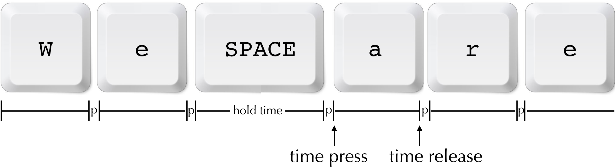
Figure 1: Keystroke logging. $p$ are pauses between keystrokes.

An example of pre-word pauses (in the remainder simply called pauses) calculated from our actual keylog data is shown in Table 1. If we take an arbitrary threshold of 500ms, the chunks indicated by the brackets are derived. This affirms that pre-word pauses carry constituency-like information.

However, typing behavior of users differs, as illustrated in Figure 2. Hence, rather than finding a global metric we rely on per-user calculated aggregate statistics and discretize them to obtain auto-derived labels, as explained next.

Token:	$[$ Coefficient	of	determination $]$	$[$ is	a $]$	$[$ measure	used	in $]$	$[$ statisitcal	model $]$	$[$ analysis $]$
Pause (ms):	0	96	496	30769	96	2144	96	80	2975	240	680

Table 1: Example keystroke log for user 33 (including typo). If we segment the data using an arbitrary 500ms pre-word pause the chunks indicated by the brackets are obtained. To normalize over idiosyncrasies of users we use per-user average statistics to obtain segments with auto-derived labels, see Section 2.1.

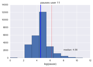
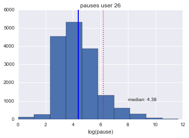
Figure 2: Distribution of pauses for two users (plotted in log space). Red solid line: per-user median pause. Dotted line: arbitrary 500ms threshold. As can be seen from the plots, the users’ typing dynamics differs.

We calculate $p$, the pause duration before a token, and bin it into the following categories, using BIO encoding, where $median$ is the per-user median and $mad$ the median absolute deviation. In this way, we automatically gather labels from keystrokes representing pause durations.

In particular, we use the following discretization, i.e., a label for a token is calculated by:

$label$ =	<m	if $p<median$;
	<m+.5	if $p<median+0.5*mad$;
	<m+1	if $p<median+mad$;
	>m1	else;
	O	for punctuation symbols.

The label is further enriched with a prefix in BIO encoding style, motivated by the fact that we want to model spans of information. Punctuation symbols are treated as O, because due to their location at boundary positions the pause information varies highly. We leave treating punctuation separately as future work.  ?) use a related encoding scheme to discretize fixation durations obtained from eye tracking data, however, in contrast to them we here use median-based measures which are better suited for such highly skewed data [Leys et al., 2013]. An actual example of automatically labeled keystroke data is given in Table 2.

B-<m	B-<m+1	B-<m	I-<m	B-<m+.5	I-<m+.5	B->m+1
the	closer	the	number	is	to	1

Table 2: Example auto-derived keystroke annotation.

2.2 Background

The major scientific interest in keystroke dynamics is that it provides a non-intrusive method for studying cognitive processes involved in writing. Keystroke logging has developed to a promising tool in writing research [Sullivan et al., 2006, Nottbusch et al., 2007, Wengelin, 2006, Van Waes et al., 2009, Baaijen et al., 2012], where time measurements—pauses, bursts and revisions (described below)—are studied as traces of the recursive nature of the writing process.

In its raw form, keystroke logs contain information on which key was pressed for how long (key, time press, time release). This data is then used to calculate between keystroke pause durations, such as pre-word pauses. It has been shown that pauses reflect the planning of the unit of text itself [Baaijen et al., 2012] and that they correlate with clause and sentence boundaries [Spelman Miller and Sullivan, 2006]. Writing research is interested in bursts of writing, defined as consecutive chunks of text produced and defined by a 2000ms time of inactivity [Wengelin, 2006], or revisions. Such a cutoff is rather arbitrary [Baaijen et al., 2012], and from our own experience results in long chunks. Taking writing research as a starting point, we postulate that keystrokes contain further fine-grained information that help identify syntactic chunks. We aim at a finer-grained representation, and transform user-based average statistics into automatically derived labels (cf. above).

We notice that the literature defines different ways to define a pause.  ?), coming from a stylometry background, use the difference between release time of the previous key and the timepress of the current key to calculate pre-word pause duration. In contrast, writing research [Wengelin, 2006, Van Waes et al., 2009, Baaijen et al., 2012] defines pauses as the start time of a keystroke until the start time of the next keystroke. We experimented with both types of pause definitions, and found the former slightly more robust, hence we use that to calculate pauses throughout this paper.

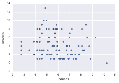
Figure 3: left: Word pauses length vs word length (left: user 7, right: user 3; Pearson $\rho=0.08$, and $\rho=-0.12$)

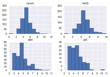
Figure 4: Word pause length distribution per part-of-speech (user 5).

In order to get a better feel of word pause durations, we examine various properties of them. First, do we need to normalize pauses for word length?  ?) found a linear relationship between pre-word pauses and word length in their dataset. We calculated the correlation between word length and pauses in our dataset, but could not observe such a relation in our data (cf. Figure 3; plots for the other participants looks similar). Even if we break the data down by POS and calculate per-POS wise correlations we found no relation between pause duration and word length. Hence we do not normalize word pause durations. In addition, Figure 4 plots pauses for various part-of-speech, showing that function POS (determiner, particles) are preceded by shorter pauses than content POS (we obtain similar plots for other participants).

Second, keystroke logs are presumably idiosyncratic, can we still use it? In fact, user keystroke biometrics are successfully used for author stylometry and verification in computer security research [Stewart et al., 2011, Monaco et al., 2013, Locklear et al., 2014]. However, also eye tracking data like scanpaths (the resulting series of fixations and saccades in eye tracking) are known to be idiosyncratic [Kanan et al., 2015]. Nevertheless it has been shown that gaze patterns help to inform NLP [Barrett and Søgaard, 2015, Klerke et al., 2016]. We believe this is also the case for biometric keystroke logging data.

3 Tagging with bi-LSTMs

We draw on the recent success of bi-directional recurrent neural network (bi-RNNs) [Graves and Schmidhuber, 2005], in particular Long Short-Term Memory (LSTM) models [Hochreiter and Schmidhuber, 1997]. They read the input sequences twice, in both directions. Bi-LSTM have recently successfully been used for a variety of tasks [Collobert et al., 2011, Ling et al., 2015, Wang et al., 2015, Huang et al., 2015, Dyer et al., 2015, Ballesteros et al., 2015, Kiperwasser and Goldberg, 2016, Liu et al., 2015]. For further details, see ?) and ?).

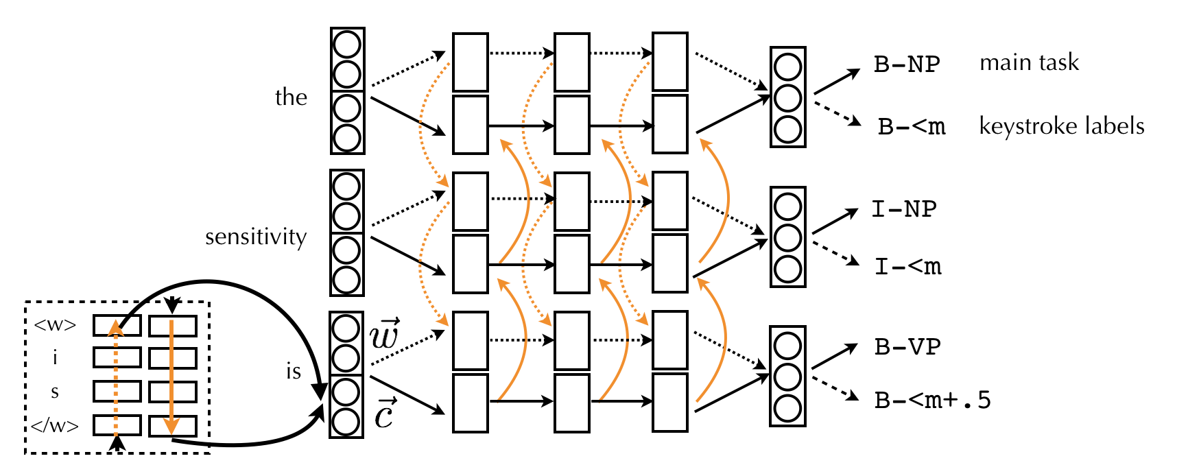
Figure 5: Hierarchical Bi-LSTM with 3 stacked layers using word $\vec{w}$ and characters $\vec{c}$ embeddings.

3.1 Bidirectional Long-Short Term Memory Models

Our model is a a hierarchical bi-LSTM as illustrated in Figure 5. It takes as input word embeddings $\vec{w}$ concatenated with character embeddings obtained from the last two states (forward, backward) of running a lower-level bi-LSTM on the characters. Adding character representations as additional information has been shown to be effective for a number of tasks, including parsing and tagging [Ballesteros et al., 2015, Gillick et al., 2015, Plank et al., 2016].

In more detail, our model is a context bi-LSTM taking as input word embeddings $\vec{w}$. Character embeddings $\vec{c}$ are incorporated via a hierarchical bi-LSTM using a sequence bi-LSTM at the lower level [Ballesteros et al., 2015, Plank et al., 2016]. The character representation is concatenated with the (learned) word embeddings $\vec{w}$ to form the input to the context bi-LSTM at the upper layers.

For the hidden layers, we use stacked LSTMs with $h$=3 layers. The 3-layer bi-LSTM and lower-level character bi-LSTM represents the shared structure between tasks. From the topmost ($h$=$3$) layer labels for the different tasks (e.g., chunking, pauses) are predicted using a softmax. In Figure 5, the main task (chunking or CCG tagging) is represented by the solid arrow, the auxiliary task (keystroke logs) is indicated by the dashed arrow.

During training, we randomly sample a task and instance, and backpropagate the loss of the current instance through the shared deep network. In this way, we learn a joint model from distinct sources. Note that we also experimented with predicting the pause durations at lower levels ($h$=1), motivated by having lower-level tasks at lower layers in the network [Søgaard and Goldberg, 2016], however, we found the setup with both tasks at the outer layer more robust. Predicting all tasks at the outermost layer is the most commonly used form of multi-task learning in neural networks [Caruana, 1998, Collobert et al., 2011].

4 Experiments

We implement our model in CNN/pycnn. For all experiments, we use the same hyperparameters, set on a held-out portion of the CoNLL 2000 data, i.e., SGD with cross-entropy loss, no mini-batches, 30 epochs, default learning rate (0.1), 64 dimensions for word embeddings, 100 for character embeddings, random initialization for all embeddings, 100 hidden states, $h=3$ stacked layers, Gaussian noise with $\sigma$=0.2. As training is stochastic, we use a fixed seed throughout (chosen and fixed upfront). No further unlabeled data is considered.

Datasets

An overview of the syntactic datasets considered in this paper is given in Table 3. For chunking, we use the original CoNLL data [Tjong Kim Sang and Buchholz, 2000] from WSJ (WSJ sections 15-18 as training data and section 20 as test data, containing 8936 and 2012 sentences, respectively). For testing we take out-of-domain data whenever available, to test the adaptability of the method to noisy out-of-domain data. For chunking we use Twitter data from ?) (all, 2364 tweets) and ?) (250 sentences), converted to chunks [Plank et al., 2014].

The CCG supertagging data also comes from WSJ (39604 training and 2407 test sentences). We unfortunately do not have access to out-of-domain test data, hence use the CCG tagging test set.

sentences	Train	Dev	Test
CoNLL 2000	8936	–	2012
Foster	–	269	250
Ritter	–	–	2364
CCG	39604	1913	2407

Table 3: Statistics on the data sets

The keystroke logging data stems from students taking an actual test on spreadsheet modeling in a university course [Stewart et al., 2011, Monaco et al., 2013]. The advantage of this dataset is that it contains free-text input. We used data from 38 users, which produced on average 250 sentences. The data totals to 7699 sentences.

To evaluate our models we use standard evaluation measures computed with conlleval.pl with default parameters, i.e., we report F1 on chunks and accuracy on CCG tags. Statistical significance is computed using the approximate randomization test [Noreen, 1989] using $i=1000$ iterations and $p$-values are reported [Søgaard et al., 2014].

4.1 Results

Chunking	F1	CCG tagging	Accuracy
Our model	93.21	Our model	92.41
?)	93.88	?)	93.00

Table 4: Baseline model, comparison to existing systems

Baseline model

Both or baseline models are comparable to prior work, while being simpler. The results are summarized in Table 4. Our chunking baseline achieves an $F1$ of 93.21 on CoNLL, compared to the $F1$ of 93.88 of ?), who use a CRF and gold POS tags. We do not use any POS information. A similar bi-LSTM achieves 93.64 [Huang et al., 2015], however, additionally uses POS embeddings. Our baseline CCG supertagging model achieves 92.41, compared to the more complex model by ?) achieving an accuracy of 93.00. Very recently even higher accuracies were reported, e.g. [Vaswani et al., 2016], however, in this exploratory paper we are interested in examining whether we find signal in keystroke data, and are not interested in beating the latest state-of-the-art.

	Foster.dev	Foster.test	Ritter	CCG
Baseline	73.93	73.61	66.65	92.41
+Pause	74.63†	74.32†	66.91†	92.62†
$p$-values	$<$0.01	$<$0.01	$<$0.01	$<$0.048

Table 5: Chunking results (F1, +Pause is average over 38 participants) and CCG accuracy (using all pause data at once). Results marked with ^† are significantly better than the corresponding baseline using a randomization test with $i=1000$ iterations; $p$-values provided in row below.

Keystroke pauses

The aim of our experiments is to gauge whether through joint learning of shallow syntax and pause duration the system learns to generalize over the pause information and thus aids the syntactic signal.

The results in Table 5 support our hypothesis that keystroke dynamics contains useful information for chunking. We here report the average over models trained on a per-user basis, i.e., 38 participants. The results show that overall F1 chunking score improves over all datasets. For instance on the Ritter data, for 25/38 participants using their keystroke information as auxiliary task helps to improve overall chunking performance. However, if we combine all data and train a single model, performance degrades on chunking. We attribute this effect to the fact that the chunking data is relatively small, and higher amounts of keystroke data show signs of overfitting. In fact, similar effects have been shown in a multi-task machine translation and parsing setup [Luong et al., 2016], where mixing coefficients were used to downplay the importance of the auxiliary parsing data that otherwise swamped the main task data. We leave examining task-specific weights for the loss for future work.

In contrast in CCG tagging, where we have more training data, we see a positive effect of using keystroke data when training a model that uses all keystroke data at once (concatenation of all keystroke data from all users), see last column in Table 5. Note that all results in Table 5 are significant.

		Foster.dev	Foster.test	Ritter
Baseline	NP	72.18	71.41	61.76
	VP	70.25	73.44	75.13
	PP	93.25	91.85	89.05
+Pause	NP	73.99	72.77	62.60
	VP	69.88	74.93	75.05
	PP	93.24	90.82	88.87

Table 6: Chunking results per label.

Label	Baseline	+Pause
N	97.20	97.27
N/N	96.38	96.62
NP[nb]/N	99.02	99.03
(NP\NP)/NP	88.41	88.95
NP	97.06	97.63
PP/NP	72.60	73.64
((S\NP)\(S\NP))/NP	72.83	74.07
conj	98.62	98.67

Table 7: CCG tagging results per label (most frequent non-punctuation labels shown).

5 Discussion

To gain better insights into what the model has learned, Table 6 provides the per-label breakdown for chunking, Table 7 for CCG tagging. Most of the improvements come from noun phrases (NP) chunks. From manual inspection we determine that the model improves particularly on non-conventional spelling and fragmented noun phrases typical for Twitter, see examples given in Table 8.

As Table 6 shows, keystroke data also helps for verb phrases on one dataset. The current encoding is not so beneficial for PPs. Pauses before prepositions are short, as illustrated in Figure 4, and pauses often fall within segments in the auxiliary annotation, while prepositions constitute separate tokens in chunking. Hence, it is unsurprising that the model fares worse on PPs.

We believe that our pause encoding mainly captures structural information between words, less morphosyntactic information itself, i.e., that pauses are more informative of syntactic structure than of part-of-speech. This intuition is in fact confirmed by initial experiments on POS tagging (UD English), which are less promising. We observe small improvements for low amounts of auxiliary data, however, they are not significant. Thus keystrokes seem to capture mostly structural shallow syntactic information, as confirmed in our experimental evaluation. However, this is only a first exploration, with one way of using keystroke logging data, but given our promising results, further experiments are warranted.

Token	Gold	Baseline	Model
Auburn	B-NP	I-NP	B-NP
party	I-NP	I-NP	I-NP
at	B-PP	B-PP	B-PP
Spurs	B-NP	B-NP	B-NP
v	B-NP	I-NP	B-VP
Man	B-NP	I-NP	B-NP
utd	I-NP	B-VP	I-NP
sounds	B-VP	B-VP	B-VP
bithcy	B-ADJP	B-VP	B-ADJP

Table 8: Selected examples from the Twitter datasets.

6 Related Work

Keystroke logging has developed into a promising tool for research into writing [Wengelin, 2006, Van Waes et al., 2009, Baaijen et al., 2012], as time measurements can give insights into cognitive processes involved in writing [Nottbusch et al., 2007] or translation studies. In fact, most prior work that uses keystroke logs focuses on experimental research. For example, ?) study whether a bilingual glossary reduces the working time of professional translators. They consider pause durations before terms extracted from keystroke logs and find that a bilingual glossary in the translation process of documentaries reduces the translators’ workload. Other translation research has combined eye-tracking data with keystroke logs to study the translation process [Carl et al., 2016]. An analysis of users’ typing behavior was studied by ?). They collect keystroke logs of online users describing images to measure spelling difficulty. They analyzed corrected and uncorrected spelling mistakes in Japanese and English and found that spelling errors related to phonetic problems remain mostly unnoticed.

?) is the only study prior to us that use keystroke loggings in NLP. In particular, they investigate the relationship between pre-word pauses and multi-word expressions and found within MWE pauses vary depending on cognitive task. We take a novel approach and learn keystroke patterns and use them to inform shallow syntactic parsing.

A recent related line of work explores eye tracking data to inform sentence compression [Klerke et al., 2016] and induce part-of-speech [Barrett and Søgaard, 2015]. Similarly, there are recent studies that predict fMRI activation from reading [Wehbe et al., 2014] or use fMRI data for POS induction [Bingel et al., 2016]. The distinct advantage of keystroke dynamics is that it is easy to get, non-expensive and non-intrusive.

7 Conclusions

Keystroke dynamics contain useful information for shallow syntactic parsing. Our model, a bi-LSTM, integrates keystroke data as auxiliary task, and outperforms models trained on the linguistic signal alone. We obtain promising results for two syntactic tasks, chunking and CCG supertagging. This warrants many directions for future research, e.g., using information from the non-linear writing process, which we here disregarded (e.g., revisions), evaluating on other languages and going to the full parsing task.

References

- [Baaijen et al., 2012] Veerle M Baaijen, David Galbraith, and Kees de Glopper. 2012. Keystroke analysis: Reflections on procedures and measures. Written Communication, page 0741088312451108.
- [Baba and Suzuki, 2012] Yukino Baba and Hisami Suzuki. 2012. How are spelling errors generated and corrected?: a study of corrected and uncorrected spelling errors using keystroke logs. In Proceedings of the 50th Annual Meeting of the Association for Computational Linguistics: Short Papers-Volume 2.
- [Ballesteros et al., 2015] Miguel Ballesteros, Chris Dyer, and Noah A. Smith. 2015. Improved transition-based parsing by modeling characters instead of words with lstms. In EMNLP.
- [Barrett and Søgaard, 2015] Maria Barrett and Anders Søgaard. 2015. Using reading behavior to predict grammatical functions. In Workshop on Cognitive Aspects of Computational Language Learning.
- [Barrett et al., 2016] Maria Barrett, Joachim Bingel, and Anders Søgaard. 2016. Part-of-speech induction from eye-tracking data. In ACL.
- [Bingel et al., 2016] Joachim Bingel, Maria Barrett, and Anders Søgaard. 2016. Part-of-speech induction from fmri. In ACL.
- [Carl et al., 2016] Michael Carl, Isabel Lacruz, Masaru Yamada, and Akiko Aizawa. 2016. Measuring the translation process. In The 22nd Annual Meeting of the Association for Natural Language Processing. NLP 2016.
- [Caruana, 1998] Rich Caruana. 1998. Multitask learning. In Learning to learn, pages 95–133. Springer.
- [Cho, 2015] Kyunghyun Cho. 2015. Natural language understanding with distributed representation. ArXiv, abs/1511.07916.
- [Collobert et al., 2011] Ronan Collobert, Jason Weston, Léon Bottou, Michael Karlen, Koray Kavukcuoglu, and Pavel Kuksa. 2011. Natural language processing (almost) from scratch. The Journal of Machine Learning Research, 12:2493–2537.
- [Dyer et al., 2015] Chris Dyer, Miguel Ballesteros, Wang Ling, Austin Matthews, and Noah A. Smith. 2015. Transition-based dependency parsing with stack long short-term memory. In ACL.
- [Foster et al., 2011] Jennifer Foster, Ozlem Cetinoglu, Joachim Wagner, Josef Le Roux, Joakim Nivre, Deirde Hogan, and Josef van Genabith. 2011. From news to comments: Resources and benchmarks for parsing the language of Web 2.0. In IJCNLP.
- [Gillick et al., 2015] Dan Gillick, Cliff Brunk, Oriol Vinyals, and Amarnag Subramanya. 2015. Multilingual language processing from bytes. arXiv.
- [Goldberg, 2015] Yoav Goldberg. 2015. A primer on neural network models for natural language processing. ArXiv, abs/1510.00726.
- [Goodkind and Rosenberg, 2015] Adam Goodkind and Andrew Rosenberg. 2015. Muddying the multiword expression waters: How cognitive demand affects multiword expression production. In Proceedings of MWE 2015.
- [Graves and Schmidhuber, 2005] Alex Graves and Jürgen Schmidhuber. 2005. Framewise phoneme classification with bidirectional lstm and other neural network architectures. Neural Networks, 18(5):602–610.
- [Hanoulle et al., 2015] Sabien Hanoulle, Véronique Hoste, and Aline Remael. 2015. The translation of documentaries: Can domain-specific, bilingual glossaries reduce the translators’ workload? an experiment involving professional translators. New Voices in Translation Studies, 23(13).
- [Hochreiter and Schmidhuber, 1997] Sepp Hochreiter and Jürgen Schmidhuber. 1997. Long short-term memory. Neural computation, 9(8):1735–1780.
- [Huang et al., 2015] Zhiheng Huang, Wei Xu, and Kai Yu. 2015. Bidirectional lstm-crf models for sequence tagging. arXiv preprint arXiv:1508.01991.
- [Kanan et al., 2015] Christopher Kanan, Dina NF Bseiso, Nicholas A Ray, Janet H Hsiao, and Garrison W Cottrell. 2015. Humans have idiosyncratic and task-specific scanpaths for judging faces. Vision research, 108:67–76.
- [Kiperwasser and Goldberg, 2016] E. Kiperwasser and Y. Goldberg. 2016. Simple and Accurate Dependency Parsing Using Bidirectional LSTM Feature Representations. ArXiv e-prints.
- [Klerke et al., 2016] Sigrid Klerke, Yoav Goldberg, and Anders Søgaard. 2016. Improving sentence compression by learning to predict gaze. In NAACL.
- [Leys et al., 2013] Christophe Leys, Christophe Ley, Olivier Klein, Philippe Bernard, and Laurent Licata. 2013. Detecting outliers: Do not use standard deviation around the mean, use absolute deviation around the median. Journal of Experimental Social Psychology, 49(4):764–766.
- [Li et al., 2012] Shen Li, João Graça, and Ben Taskar. 2012. Wiki-ly supervised part-of-speech tagging. In EMNLP.
- [Ling et al., 2015] Wang Ling, Chris Dyer, Alan W Black, Isabel Trancoso, Ramon Fermandez, Silvio Amir, Luis Marujo, and Tiago Luis. 2015. Finding function in form: Compositional character models for open vocabulary word representation. In EMNLP.
- [Liu et al., 2015] Pengfei Liu, Shafiq Joty, and Helen Meng. 2015. Fine-grained opinion mining with recurrent neural networks and word embeddings. In EMNLP.
- [Locklear et al., 2014] Hilbert Locklear, Sathya Govindarajan, Zdenka Sitova, Adam Goodkind, David Guy Brizan, Andrew Rosenberg, Vir V Phoha, Paolo Gasti, and Kiran S Balagani. 2014. Continuous authentication with cognition-centric text production and revision features. In Biometrics (IJCB), 2014 IEEE International Joint Conference on.
- [Luong et al., 2016] Minh-Thang Luong, Quoc V. Le, Ilya Sutskever, Oriol Vinyals, and Lukasz Kaiser. 2016. Multi-task sequence to sequence learning. In ICLR.
- [Monaco et al., 2013] John V Monaco, John C Stewart, Sung-Hyuk Cha, and Charles C Tappert. 2013. Behavioral biometric verification of student identity in online course assessment and authentication of authors in literary works. In Biometrics: Theory, Applications and Systems (BTAS), 2013 IEEE Sixth International Conference on, pages 1–8. IEEE.
- [Noreen, 1989] Eric Noreen. 1989. Computer-intensive methods for testing hypotheses: an introduction. Wiley.
- [Nottbusch et al., 2007] Guido Nottbusch, Rüdiger Weingarten, and Said Sahel. 2007. From written word to written sentence production. Writing and cognition: Research and applications., pages 31–54.
- [Plank et al., 2014] Barbara Plank, Dirk Hovy, and Anders Søgaard. 2014. Learning part-of-speech taggers with inter-annotator agreement loss. In EACL.
- [Plank et al., 2016] Barbara Plank, Anders Søgaard, and Yoav Goldberg. 2016. Multilingual part-of-speech tagging with bidirectional long short-term memory models and auxiliary loss. In ACL.
- [Plank, 2016] Barbara Plank. 2016. What to do about non-standard (or non-canonical) language in NLP. In KONVENS.
- [Ritter, 2011] Alan Ritter. 2011. Extracting Knowledge from Twitter and The Web. Ph.D. thesis, University of Washington.
- [Søgaard and Goldberg, 2016] Anders Søgaard and Yoav Goldberg. 2016. Deep multi-task learning with low level tasks supervised at lower layers. In ACL.
- [Søgaard et al., 2014] Anders Søgaard, Anders Johannsen, Barbara Plank, Dirk Hovy, and Héctor Martínez Alonso. 2014. What’s in a p-value in nlp? In CoNLL.
- [Spelman Miller and Sullivan, 2006] Kristyan Spelman Miller and Kirk PH Sullivan. 2006. Keystroke logging: an introduction. Elsevier.
- [Stewart et al., 2011] John C Stewart, John V Monaco, Sung-Hyuk Cha, and Charles C Tappert. 2011. An investigation of keystroke and stylometry traits for authenticating online test takers. In Biometrics (IJCB), 2011 International Joint Conference on, pages 1–7. IEEE.
- [Sullivan et al., 2006] Kirk PH Sullivan, Eva Lindgren, et al. 2006. Computer keystroke logging and writing: Methods and applications. Elsevier.
- [Suzuki and Isozaki, 2008] Jun Suzuki and Hideki Isozaki. 2008. Semi-supervised sequential labeling and segmentation using giga-word scale unlabeled data. In ACL.
- [Tjong Kim Sang and Buchholz, 2000] Erik Tjong Kim Sang and Sabine Buchholz. 2000. Introduction to the conll-2000 shared task: Chunking. In CoNLL.
- [Van Waes et al., 2009] Luuk Van Waes, Mariëlle Leijten, and Daphne Van Weijen. 2009. Keystroke logging in writing research: Observing writing processes with inputlog. GFL-German as a foreign language, 2(3):41–64.
- [Vaswani et al., 2016] Ashish Vaswani, Yonatan Bisk, Kenji Sagae, and Ryan Musa. 2016. Supertagging with lstms. In NAACL.
- [Wang et al., 2015] Peilu Wang, Yao Qian, Frank K. Soong, Lei He, and Hai Zhao. 2015. Part-of-speech tagging with bidirectional long short-term memory recurrent neural network. pre-print, abs/1510.06168.
- [Wehbe et al., 2014] Leila Wehbe, Ashish Vaswani, Kevin Knight, and Tom Mitchell. 2014. Aligning context-based statistical models of language with brain activity during reading. In EMNLP.
- [Wengelin, 2006] Åsa Wengelin. 2006. Examining pauses in writing: Theory, methods and empirical data. Computer key-stroke logging and writing: methods and applications (Studies in Writing), 18:107–130.
- [Xu et al., 2015] Wenduan Xu, Michael Auli, and Stephen Clark. 2015. Ccg supertagging with a recurrent neural network. In ACL.