Characterizing the $\gamma$-ray long-term variability of PKS 2155$-$304 with H.E.S.S. and Fermi LAT

Studying the temporal variability of BL Lac objects at the highest energies provides unique insights into the extreme physical processes occurring in relativistic jets and in the vicinity of super-massive black holes. To this end, the long-term variability of the BL Lac object PKS 2155$-$304 is analyzed in the high (HE, $100\,$MeV$<E<300\,$GeV) and very high energy (VHE, $E>200\,$GeV) $\gamma$-ray domain. Over the course of $\sim 9\,$yr of H.E.S.S. observations the VHE light curve in the quiescent state is consistent with a log-normal behavior. The VHE variability in this state is well described by flicker noise (power-spectral-density index $\beta_{\textrm{VHE}}=1.10^{+0.10}_{-0.13}$) on time scales larger than one day. An analysis of $\sim 5.5$ yr of HE Fermi LAT data gives consistent results ($\beta_{\textrm{HE}}=1.20^{+0.21}_{-0.23}$, on time scales larger than 10 days) compatible with the VHE findings. The HE and VHE power spectral densities show a scale invariance across the probed time ranges. A direct linear correlation between the VHE and HE fluxes could neither be excluded nor firmly established. These long-term-variability properties are discussed and compared to the red noise behavior ($\beta\sim 2$) seen on shorter time scales during VHE-flaring states. The difference in power spectral noise behavior at VHE energies during quiescent and flaring states provides evidence that these states are influenced by different physical processes, while the compatibility of the HE and VHE long-term results is suggestive of a common physical link as it might be introduced by an underlying jet-disk connection.

1 Introduction

One of the most striking properties of BL Lacertae objects is their variability across the electromagnetic spectrum from radio to $\gamma$ rays and accros the temporal spectrum from minutes to years. In the current standard paradigm of active galactic nuclei (e.g., Urry & Padovani, 1995) the observed nonthermal emission is produced in two-sided collimated, relativistic plasma outflows (jets) closely aligned with the line of sight, so that the intrinsic emission appears enhanced because of Doppler-boosting effects. The jets are powered by a central engine consisting of a supermassive black hole surrounded by an accretion disk. Characterizing the temporal variability provides one of the key diagnostics for the physical conditions in these systems, for example the jet-disk connection, location of the emitting region, or dominant emission processes.

The BL Lac PKS 2155$-$304 (redshift $z=0.116$; Falomo et al., 1993) has been observed with the High Energy Stereoscopic System (H.E.S.S.; Hinton, 2004) at very high-energy $\gamma$-rays (VHE; $E>200$ GeV) since 2002 (e.g., Abramowski et al., 2010, and references therein). The source underwent an extreme VHE flux outburst in July/August 2006 with peak fluxes exceeding the average flux level of the long-term emission by a factor of $\sim$ $100$, during which it showed rapid variability on timescales as short as 3 min (Aharonian et al., 2007). The stochastic VHE variability during this flaring state has been characterized as power-law noise ($\propto f^{-\beta}$, where $f$ is the frequency) with an index $\beta\sim 2$. A detailed analysis of the VHE data from 2005-2007 revealed that the run-by-run light curve of PKS 2155$-$304 follows a skewed flux distribution, which is well represented by two superposed lognormal distributions (Abramowski et al., 2010, Fig. 3). Excluding the flare data, the flux distribution satisfies a simple lognormal distribution. This provides evidence that the source switches from a quiescent VHE state with minimal activity to a flaring state, and the flux distribution in each state follows a lognormal distribution. Lognormal behavior was first established for accreting Galactic sources such as X-ray binaries by Uttley & McHardy (2001), linking such a behavior to the underlying accretion process. In a lognormal process, the fluctuations of the flux are on average proportional, or at least correlated, to the flux itself, ruling out additive processes in favor of multiplicative processes. In the case of blazars, a lognormal behavior could thus mark the influence of the accretion disk on the jet (e.g., Giebels & Degrange, 2009; McHardy, 2010). Cascade-like events are an example of multiplicative lognormal processes. Density fluctuations in the accretion disk provide one possible realization. If damping is negligible, these fluctuations can propagate inward and couple together to produce a multiplicative behavior. If this is efficiently transmitted to the jet, the $\gamma$-ray emission could be modulated accordingly.

In Sect. 2 we present VHE data from $9$ years of H.E.S.S. observations of PKS 2155$-$304 in the quiescent state, and partially contemporaneous HE data from $5.5$ years of observations from the Large Area Telescope (Fermi LAT), are presented in Sec. 2. In Sect. 3, a detailed time-series analysis is performed. First, the light curves are tested for a lognormal behavior. Then, their variability is characterized as power-law noise with a forward folding method with simulated light curves, taking the sampling of the data, described in Kastendieck et al. (2011) into account. And, finally, the VHE and HE emissions are also analyzed for a possible direct linear correlation. This is the first time that such an extended analysis is performed on the VHE $\gamma$-ray emission of a BL Lac object on timescales as long as nine years. In Sect. 4 the results of the two energy ranges are compared and their implications on the physical properties of PKS 2155$-$304 are discussed.

2 Observations and analysis

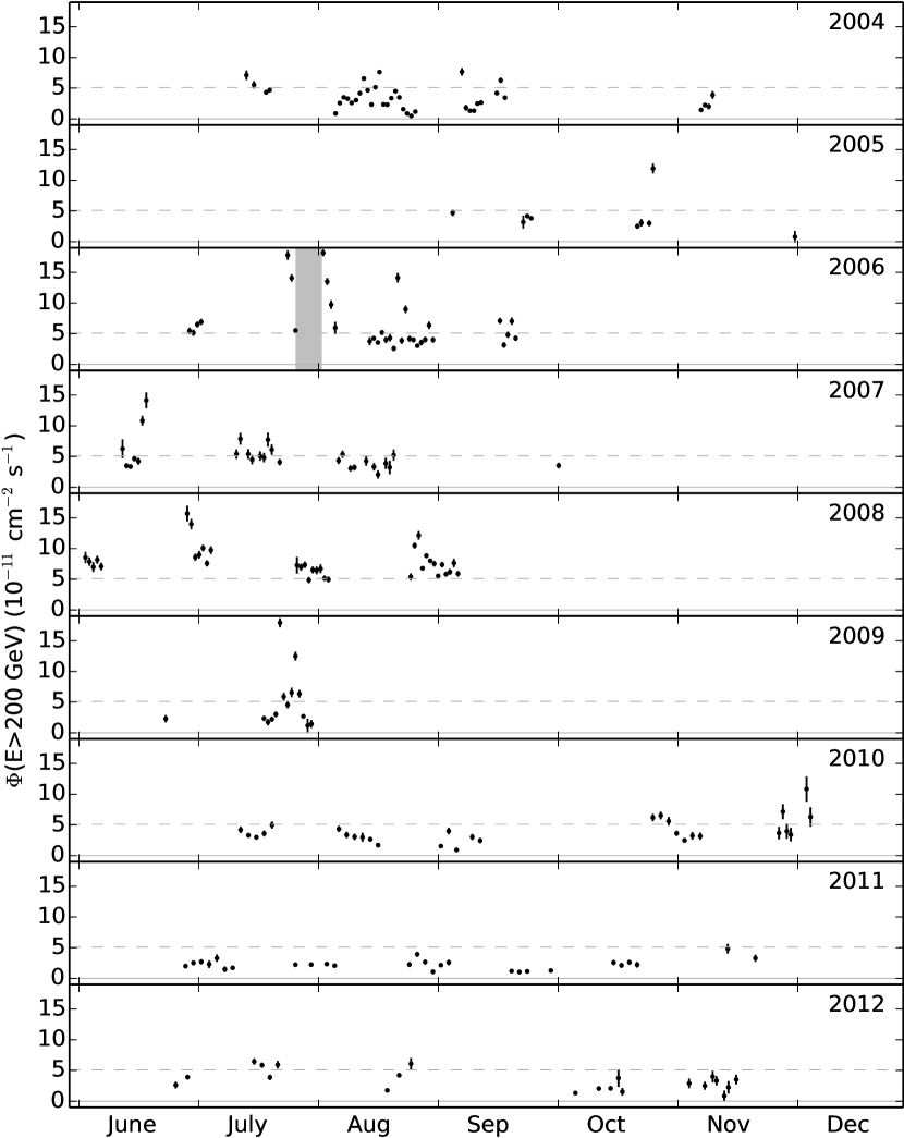
Figure 1: H.E.S.S. light curve of nightly fluxes above 200 GeV excluding the high state in July/August 2006 (gray shaded area). The gray dashed horizontal line indicates the average flux of the quiescent state.

H.E.S.S. (VHE):

H.E.S.S. is an array of five Imaging Atmospheric Cherenkov Telescopes (IACTs). The first phase of H.E.S.S. began in 2003 with four 12-meter telescopes giving an energy threshold $\sim$ $100$ GeV. In 2012, a fifth 28-meter telescope was added to the array, reducing the energy threshold to $\sim$ $50$ GeV.

The present analysis is based on VHE data taken with the completed H.E.S.S. Phase-I between MJD $53200$ (14 July 2004) and $56246$ (15 November 2012), using three or four telescopes. The high flux state from 27 July to 8 August 2006, with an average flux of $(75.2\pm 0.8)\times 10^{-11}$ cm^-2 s^-1 above $200$ GeV is excluded from the data set. The remaining data constitutes the basis for the time-series analysis, and is referred to as the quiescent data set in the following.

In total, about $328\,$h of data passed standard quality cuts as defined in Aharonian et al. (2006), with a mean zenith angle of $21^{\circ}$ resulting in an average energy threshold of $178\,$GeV. The data set has been analyzed with the Model analysis chain using standard cuts (de Naurois & Rolland, 2009) above $200$ GeV.

The total detection significance in the quiescent data set corresponds to $341\,\sigma$. The light curve of nightly fluxes is calculated assuming a log-parabolic energy spectrum,

$$\centering{\rm d}N/{\rm d}E\propto E^{-a-b\log E},\@add@centering$$ (1)

with $a$ and $b$ corresponding to the best-fit power-law index and curvature index, respectively. In order to take indications of a spectral variability in the VHE domain during the quiescent state (Abramowski et al., 2010) into account, the nightly fluxes are derived with a separate log-parabola fit of the spectrum for each year.

The values for $a$ and $b$ are summarized in Table 1; the average values are $\overline{a}=3.209$ and $\overline{b}=0.164$. The unbiased sample variance for the first parameter

$$s_{a}^{2}=\frac{1}{n-1}\sum_{i=1}^{n}\left(a_{i}-\overline{a}\right)^{2}=0.017$$ (2)

is larger than the expected variance $\overline{\sigma_{a}^{2}}=0.005$ because of the uncertainties $\sigma_{a}$ on the individual best-fit values. The same is true for the second parameter with $s_{b}^{2}=0.114$ and $\overline{\sigma_{b}^{2}}=0.005$. This could be indicative of a variable spectrum.

Table 1: Values of the log-parabola parameters of the spectrum (Eq. 1) of PKS 2155$-$304 used to derive the light curve.

Year	$a\pm\sigma_{a}$	$b\pm\sigma_{b}$
2004	$2.95\pm 0.03$	$0.37\pm 0.03$
2005	$3.27\pm 0.12$	$0.25\pm 0.12$
2006	$3.27\pm 0.04$	$0.24\pm 0.04$
2007	$3.38\pm 0.08$	$-0.03\pm 0.07$
2008	$3.28\pm 0.04$	$0.12\pm 0.03$
2009	$3.14\pm 0.08$	$0.18\pm 0.07$
2010	$3.24\pm 0.08$	$0.10\pm 0.07$
2011	$3.08\pm 0.10$	$0.13\pm 0.08$
2012	$3.27\pm 0.01$	$0.12\pm 0.09$

Variations within a season, however, are unlikely to affect the analysis presented here as the inferred small changes in the spectral parameters only result in small changes in the integral flux.

The resulting quiescent light curve has an average flux of $(5.10\pm 0.41)\times 10^{-11}\,\mathrm{cm}^{-2}\,\mathrm{s}^{-1}$ above 200 GeV and is shown in Fig. 1. It is characterized by a fractional root mean square variability (Vaughan et al., 2003)

$$F_{\rm var}={\sqrt{S_{\Phi}^{2}-\overline{\sigma_{\rm err}^{2}}}\over\overline{\Phi}}=0.66\pm 0.01,$$ (3)

where $\overline{\Phi}$ is the mean flux, $S_{\Phi}^{2}$ is the variance of the fluxes and $\overline{\sigma_{\rm err}^{2}}$ is the contribution to the variance caused by the measurement errors. The analysis results were cross-checked using different analysis methods and calibration chains (e.g., Aharonian et al., 2006), yielding compatible results.

Fermi LAT (HE):

Figure 2: Light curve of the integral fluxes between $0.1$ and $300\,$GeV in bins of ten days measured with Fermi LAT. The dashed line indicates the average flux.

The Fermi LAT (Atwood et al., 2009) on board the Fermi satellite is a pair-conversion telescope designed to detect HE $\gamma$-rays in the energy range from below $20\,$MeV to more than $300\,$GeV.

The set of observational data for PKS 2155$-$304 used here covers about $5.5$ years, from MJD $54688$ (10 August 2008) to $56688$ (31 January 2014). Events are selected between 100 MeV and 300 GeV in a region of interest (ROI) of $15\hbox{${}^{\circ}$}$ around PKS 2155$-$304. The detector is described by the P7REP_SOURCE_V15 instrument response function. The HE light curve is obtained with the tool Enrico (Sanchez & Deil, 2013) using the Fermi Science Tools v9r32p5, with a 10-day binning to ensure enough statistics in each bin. The prefactor of the diffuse galactic background (gll_iem_v05) and the normalization of the isotropic diffuse emission (iso_source_v05) are left free to vary in the likelihood fit.

All sources from the third LAT source catalog (3FGL; Acero et al., 2015) within $15\hbox{${}^{\circ}$}$ of PKS 2155$-$304 are included in the model to ensure a good background modeling. The HE spectra of PKS 2155$-$304 and all sources within $3\hbox{${}^{\circ}$}$ are fitted following the spectral shape of the 3FGL catalog. The spectra of PKS 2155$-$304, 3FGL J2151.6-2744 and 3FGL J2159.2-2841 are modeled with a simple power law, while for 3FGL J2151.8-3025 a log-parabolic shape is assumed. The indices and pre-factors are left free. All other components are fixed to the values in the 3FGL catalog. PKS 2155$-$304 is detected with a significance of $156\,\sigma$ with a spectral index of $1.83\pm 0.01$. The photon counts of PKS 2155$-$304 are integrated into $201$ bins of ten days. The resulting light curve has an average flux of $1.20\pm 0.03\times 10^{-7}\,\mathrm{cm}^{-2}\,\mathrm{s}^{-1}$ between 100 MeV and 300 GeV with a $F_{\rm var}=0.41\pm 0.02$ (Eq. 3) and is shown in Fig. 2.

3 Time-series analysis

To characterize the long-term variability of PKS 2155$-$304, the HE and VHE data sets are analyzed with respect to lognormality and power-law noise.

Lognormality: A possible lognormal behavior of PKS 2155$-$304 is investigated by examining the distribution of the fluxes and studying the correlation between the flux levels and the intrinsic variability. The flux and log-flux distributions of each light curve are fitted by a Gaussian using a $\chi^{2}$ fit. The goodness of the fits are summarized in Table 2. In both cases, a Gaussian fits the log-flux distribution better than the flux distribution, with a significance level of $\sigma>5$ for the VHE and $\sigma>2$ for the HE data, respectively. For the VHE data the probability representing the goodness of fit is about $10^{4}$ times higher for the log-flux distribution when compared to the flux distribution. For the HE data this ratio is on the order of $10$. Thus, while the HE $\gamma$-ray flux of PKS 2155$-$304 in this approach shows only an indication, the VHE $\gamma$-ray flux data provide evidence for a lognormal behavior.

Table 2: Values of the reduced $\chi^{2}$ and associated probability for the Gaussian fits of the flux and log flux distributions for each light curve. The parameter $\sigma$ is the significance level on which a lognormal distribution is preferred to a normal distribution.

	$\Phi$		log $\Phi$
	$\chi^{2}/$d.o.f.	Prob	$\chi^{2}/$d.o.f.	Prob	$\sigma$
H.E.S.S.	50.8/17	$10^{-5}$	11.9/13	0.54	5.39
Fermi	21.6/12	0.04	15.0/11	0.18	2.57

In addition, the variability-flux relation, estimated by the excess RMS (root mean square; Eq. 4), is investigated for a possible correlation (Uttley et al., 2005). The excess RMS estimates the intrinsic variability of a time series by subtracting the contribution of the measurement errors. It is defined as

$$\sigma_{\rm XS}=\sqrt{S^{2}-\overline{\sigma_{\rm err}^{2}}}$$ (4)

where $S^{2}$ is the variance and $\overline{\sigma_{\rm err}^{2}}$ the mean square of the statistical error of the data (Vaughan et al., 2003). Here $\sigma_{\rm XS}$ is calculated for bins of the light curves each containing at least 20 light curve points. They are plotted versus the average fluxes $\overline{\Phi}$ of the corresponding bins for both light curves in Fig. 3.

To test the possible correlation between the flux and its variability, the scatter plots are fitted by a constant as well as a linear ascending slope. The fit results are summarized in Table 3. The results reveal a preference greater than $6\sigma$ for the linear fit to the VHE data while HE data only show an indication of linearity. To characterize this behavior beyond the fit of a linear correlation, the nonparametric correlation factor Spearman $\rho$ and the Kendall rank $\tau$, which measure the ordering of the points, (Gleissner et al., 2004) are calculated. In all cases $\rho>0.85$ and $\tau>0.65$, meaning that $\sigma_{\rm XS}$ and $\overline{\Phi}$ show a strong correlation. This implies that the fluctuations of the flux are in fact correlated with the flux.

Table 3: Values of the reduced $\chi^{2}$ of the constant and linear fits of the scatter plots shown in Fig. 3 for each light curve with values for the significance $\sigma$, correlation factor $\rho$, and Kendall rank $\tau$.

	constant	linear increase
	$\chi^{2}/$d.o.f.	$\chi^{2}/$d.o.f.	$\sigma$
H.E.S.S.	5.78	0.89	6.33
Fermi	0.936	0.107	2.75
	$\rho$	$\tau$
H.E.S.S.	$0.86\pm 0.11$	$0.78\pm 0.26$
Fermi	$0.93\pm 0.19$	$0.69\pm 0.25$

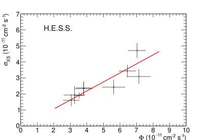
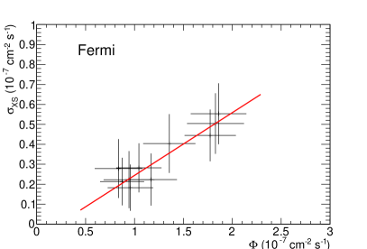
Figure 3: Scatter plot of the excess RMS and the average flux for the H.E.S.S. (left) and Fermi LAT (right) data. Each flux and excess rms values are computed using at least 20 adjacent light curve points. A linear fit is shown in red.

The preceding analysis shows that the HE and VHE flux distributions of PKS 2155$-$304 during the quiescent state are compatible with lognormal distributions. When the two energy bands are compared, the lognormal behavior is much more evident in the VHE data set. In addition, for both energy bands the variability amplitude of the flux is correlated with the flux level, supporting the conclusion that lognormality is an intrinsic characteristic of the long-term $\gamma$-ray emission in PKS 2155$-$304. A similar result has also been reported for the VHE flaring state of PKS 2155$-$304 in 2006 (Abramowski et al., 2010).

Power-law noise: The flux variability of active galaxies has frequently been characterized as power-law noise (e.g., Lawrence & Papadakis, 1993). The power spectral density (PSD), i.e., the square modulus of the discrete Fourier transform (Priestley, 1967), of such a light curve follows a power law $\propto f^{-\beta}$, where $f$ is the temporal frequency and usually $1\lower 2.15277pt\hbox{$\;\buildrel<\over{\sim}\;$}\beta\lower 2.15277pt\hbox{$\;\buildrel<\over{\sim}\;$}2$. The PSD reveals how the variability amplitude is distributed among the timescales. In a power-law noise light curve ($\beta>0$) the flux variations on longer timescales dominate the variations on shorter timescales. The total variance of such a light curve tends to grow with its length. For $\beta=0$ the variability power is equal on each time cale, resulting in white noise, where the fluxes at all times are uncorrelated.

To study the variability characteristics, we first hypothesize that the light curves can be described by power-law noise with a lognormal behavior with $\beta\geq 0$ as the only free parameter. Three different methods are then used to characterize the variability of the light curves: The Lomb-Scargle Periodogram (LSP), which is a method to approximate the PSD (Lomb, 1976; Scargle, 1982); the first-order Structure Function (SF; Simonetti et al., 1985) and the Multiple Fragments Variance Function (MFVF; Kastendieck et al., 2011), which are both representations of the PSD in the time domain.

A forward-folding method with sets of $10^{4}$ simulated light curves for each value of $\beta$ and a maximum likelihood estimator are applied to estimate the best-fit parameter $\beta$, as described in Kastendieck et al. (2011). The light curves are simulated with a lognormal behavior, so that the logarithm of the intrinsic light curve $\Phi_{\rm intr}$ is power-law noise with a Gaussian behavior of mean $\mu$ and standard deviation $\sigma$.

$$\log(\Phi_{\rm intr})\mapsto\mathcal{N}(\mu,\sigma)$$ (5)

The PSD of the simulated power-law noise is generated on a frequency range $\left[(10T)^{-1},\,5\mathrm{d}^{-1}\right]$ where $T_{\textrm{H.E.S.S.}}=3047\,$d and $T_{Fermi}=2000\,$d are the lengths of the measured light curves, respectively. The power-law noise is rebinned to ten days for the Fermi LAT analysis corresponding to the binning of the PKS 2155$-$304 light-curve. The light curves are then downsampled to the real observation times, the fluxes are rescaled to the average and variance of the measured fluxes, and measurement errors are simulated. The parameter space is sampled with $\beta=0.0,0.1,\dots,3.0$. The SFs, LSPs and MFVFs are equally binned in $\mathrm{log}_{10}$ scale with $50$, $20$, and $5$ bins per decade, respectively.

Owing to the binning, the smallest resolvable timescale in the Fermi LAT light curve is $\tau_{0}=10\,$d and the corresponding frequency is $f_{\textrm{high}}=(2\tau_{0})^{-1}=(20\,\mathrm{d})^{-1}$. For the H.E.S.S. light curve the smallest resolvable timescale is $\tau_{0}=1\,$d corresponding to $f_{\textrm{high}}=(2\,\mathrm{d})^{-1}$. The LSPs are characterized on a frequency range $\left[10^{-4}\,\mathrm{d}^{-1},f_{\textrm{high}}\right]$, while the lowest timescale for the SFs and MFVFs is $\tau_{0}$. The methods are also sensitive to variations that occur on timescales larger than the lengths of the light curves and that appear as long-term trends. It is therefore also useful to calculate the LSP on frequencies $<T^{-1}$ to reveal such information.

The application of these methods to the H.E.S.S. light curve in the quiescent state gives best-fit parameters

$$\beta_{\mathrm{LSP}}=1.10^{+0.14}_{-0.16},\quad\beta_{\mathrm{SF}}=1.00^{+0.11}_{-0.15},\quad\beta_{\mathrm{MFVF}}=1.10^{+0.10}_{-0.13}.$$

A goodness of fit test is applied where the maximum likelihood values of simulated LSPs, SFs and MFVFs, respectively, are used as test statistics. For this, new simulated sets of $10^{4}$ light curves of the best-fit parameters are analyzed with the likelihood estimator. The distribution of their maximum likelihood values is compared with the respective value of PKS 2155$-$304. Assuming the model to be correct, the values should be compatible. The quantile that has a smaller likelihood than the PKS 2155$-$304 data is used to estimate the p-value $p$. The smallest value of $p=11\%$ is found with the MFVF. The hypothesis that the data can be described by a single power-law noise model is thus not rejected.

The MFVF gives the most precise value, which is taken here as the final value:

$$\beta_{\textrm{VHE}}=1.10^{+0.10}_{-0.13}.$$

The best-fit values of the other methods are compatible within the uncertainties.

The LSP, SF and MFVF of the measured light curves together with the probability density functions (PDF) of the simple power-law noise model that best fits the data are shown in Fig. 4. The probability is normalized to unity in each frequency bin. The uncertainties of $\beta$ are found with the distributions illustrated in Fig. 5.

For comparison, as a second hypothesis, an extended model is investigated: a maximum timescale is considered, above which the variance does not increase any further. The existence of such a timescale is expected, as otherwise the variance of the light curve and therefore the flux would increase to infinity with time. This is represented by a break in the PSD to a constant level ($\beta=0$) at the corresponding frequency $f_{\mathrm{min}}$, which is treated as an additional free parameter, with a sampling $\textrm{log}_{10}\left(f_{\mathrm{min}}/\mathrm{d}^{-1}\right)=-4.4,-4.2,\dots,-1.0$.

The likelihood estimators with the three methods give best-fit values or $1\sigma$ upper limits,

$$\beta_{\mathrm{LSP}}=1.10^{+0.28}_{-0.09},$$

$$\mathrm{log}_{10}\left(f_{\mathrm{min,LSP}}/\mathrm{d}^{-1}\right)=-3.80^{+1.12}_{-0.31}<-2.68,$$

$$\beta_{\mathrm{SF}}=1.00^{+0.24}_{-0.07},$$

$$\mathrm{log}_{10}\left(f_{\mathrm{min,SF}}/\mathrm{d}^{-1}\right)=-3.80^{+1.61}_{-0.18}<-2.19,$$

$$\beta_{\mathrm{MFVF}}=1.10^{+0.23}_{-0.06},$$

$$\mathrm{log}_{10}\left(f_{\mathrm{min,MFVF}}/\mathrm{d}^{-1}\right)=-3.60^{+1.41}_{-0.34}.$$

The best-fit values of $\mathrm{log}_{10}\left(f_{\mathrm{min}}/\mathrm{d}^{-1}\right)=-3.80$ for the LSP and SF is near the formal limit of our analysis, which is constrained to $-4.4$ by the lengths of the simulated light curves. The results together with the $1\,\sigma$ uncertainties to higher values ($+1.12$ and $+1.61$) are therefore treated as $1\,\sigma$ upper limits. The best likelihood for the MFVF is given for a break in the PSD. However, the goodness-of-fit p value of $10\%$ is not improved compared to $11\%$ for the first hypothesis (assuming no break). This and the LSP and MFVF findings thus do not reveal any preference for the existence of such a break in the sampled frequency range.

An analogous analysis is performed on the Fermi LAT light curve. The following best-fit parameters for the simple power-law model are compatible:

$$\beta_{\mathrm{LSP}}=1.10^{+0.26}_{-0.31},\quad\beta_{\mathrm{SF}}=1.20^{+0.22}_{-0.31},\quad\beta_{\mathrm{MFVF}}=1.20^{+0.21}_{-0.23},$$

The most constraining result, again given by the MFVF, is taken as the final value:

$$\beta_{\textrm{HE}}=1.20^{+0.21}_{-0.23}.$$

The goodness-of-fit tests yield p values $>6\%$. Inspection of the LSP plot in Fig. 4 for the Fermi LAT data reveals a peak at $\sim(670-700)$ days, which is indicative of a possible HE periodicity on the noted timescale and influencing the p value for this analysis. It is interesting to note that a tentative HE periodicity of $\sim(620-660)$ days has already been reported (Sandrinelli et al., 2014).

(a) H.E.S.S.

(b) Fermi LAT

Figure 4: LSPs, SFs, and MFVFs. Left panel (a): The red solid lines are the LSP (top), SF (middle), and MFVF (bottom) for the H.E.S.S. quiescent light-curve. The best-fit PDFs of simulated LSP, SF, and MFVF values are represented by the blue histograms in color scale. Right panel (b): Same plots for the Fermi LAT data.

(a) H.E.S.S.

(b) Fermi LAT

Figure 5: Uncertainties on the LSP, SF, and MFVF best-fit parameters. Left panel (a): The histograms represent the distributions of estimates for $\beta$ for simulated H.E.S.S. light curves with the LSP (top), SF (middle), and MFVF (bottom) respectively. For the simulated light curves, the true value for $\beta$ is the best-fit value found for the H.E.S.S. light curve. The vertical red bars are the $1\sigma$ uncertainties on the best fit obtained from the histograms by removing equal tails. Right panel (b): Same plots for the Fermi LAT data.

A comparative analysis of the extended model (power law with a break) gives compatible results with

$$\beta_{\mathrm{LSP}}=1.10^{+0.46}_{-0.11},$$

$$\mathrm{log}_{10}\left(f_{\mathrm{min,LSP}}/\mathrm{d}^{-1}\right)=-4.20^{+1.42}_{-0.12}<-2.78,$$

$$\beta_{\mathrm{SF}}=1.20^{+0.44}_{-0.11},$$

$$\mathrm{log}_{10}\left(f_{\mathrm{min,SF}}/\mathrm{d}^{-1}\right)=-4.20^{+1.40}_{-0.12}<-2.80,$$

$$\beta_{\mathrm{MFVF}}=1.30^{+0.54}_{-0.08},$$

$$\mathrm{log}_{10}\left(f_{\mathrm{min,MFVF}}/\mathrm{d}^{-1}\right)=-3.40^{+0.74}_{-0.12}.$$

The best-fit values for the LSP and the SF are both $\mathrm{log}_{10}\left(f_{\mathrm{min}}/\mathrm{d}^{-1}\right)=-4.20$. Including the $1\,\sigma$ uncertainties to higher values ($+1.42$ and $+1.40$) they are treated as $1\,\sigma$ upper limits.

The goodness-of-fits do not improve. The results therefore give no indication for the presence of a break frequency in the PSD in the sampled frequency range. See Table 4 for a summary of these and related results.

Correlations: The VHE and HE light curves are furthermore analyzed for a possible direct correlation with the discrete correlation function (DCF; Edelson & Krolik, 1988) using a binning of $30\,$d. The results are compared with the DCFs of simulated H.E.S.S. and Fermi LAT light curves following one of the two hypotheses: (1) The H.E.S.S. and the Fermi LAT light curves are characterized by flicker noise ($\beta=1.1$) without any correlation. (2) The fluxes of such light curves obey a perfect, direct linear correlation.

For each hypothesis $10^{4}$ pairs of corresponding light curves are simulated and their DCFs are calculated. These DCFs are then combined in a two-dimensional histogram which is treated as a PDF. The hypotheses are tested according to the goodness-of-fit test described above: for the measured DCF the likelihood is calculated with the PDF. Also for the simulated DCFs the likelihoods are calculated and are used as a test statistic for calculating the p value. Both hypotheses are compatible with the measured data with p values for (1) of $41\%$, and for (2) of $59\%$, respectively. Accordingly, these results neither give a clear preference nor do they allow the rejection of a direct correlation.

Table 4: Characteristics of the power spectral densities of PKS 2155$-$304 at different energies and timescales.

Energy	Instrument	Range of	Method	$\beta$	$\textrm{log}_{10}\left(f_{\textrm{min}}/\mathrm{d}^{-1}\right)$	Goodness	Ref.
range		$\textrm{log}_{10}\left(f/\mathrm{d}^{-1}\right)$				of fit
$>200\,\textrm{GeV}$	H.E.S.S.	$\left[-4.0,-0.3\right]$	LSP, FF	$1.10^{+0.14}_{-0.16}$	no break (fixed)	56%
$>200\,\textrm{GeV}$	H.E.S.S.	$\left[-3.5,0.0\right]$	SF, FF	$1.00^{+0.11}_{-0.15}$	no break (fixed)	48%
$>200\,\textrm{GeV}$	H.E.S.S.	$\left[-3.5,0.0\right]$	MFVF, FF	$1.10^{+0.10}_{-0.13}$	no break (fixed)	11%
$>200\,\textrm{GeV}$	H.E.S.S.	$\left[-4.0,-0.3\right]$	LSP, FF	$1.10^{+0.28}_{-0.09}$	$-3.80^{+1.12}_{-0.31}<-2.68$	51%
$>200\,\textrm{GeV}$	H.E.S.S.	$\left[-3.5,0.0\right]$	SF, FF	$1.00^{+0.24}_{-0.07}$	$-3.80^{+1.61}_{-0.18}<-2.19$	43%
$>200\,\textrm{GeV}$	H.E.S.S.	$\left[-3.5,0.0\right]$	MFVF, FF	$1.10^{+0.23}_{-0.06}$	$-3.60^{+1.41}_{-0.34}$	10%
$0.1-300\,\textrm{GeV}$	Fermi LAT	$\left[-4.0,-1.3\right]$	LSP, FF	$1.10^{+0.26}_{-0.31}$	no break (fixed)	6.3%
$0.1-300\,\textrm{GeV}$	Fermi LAT	$\left[-3.3,-1.0\right]$	SF, FF	$1.20^{+0.22}_{-0.31}$	no break (fixed)	46%
$0.1-300\,\textrm{GeV}$	Fermi LAT	$\left[-3.3,-1.0\right]$	MFVF, FF	$1.20^{+0.21}_{-0.23}$	no break (fixed)	40 %
$0.1-300\,\textrm{GeV}$	Fermi LAT	$\left[-4.0,-1.3\right]$	LSP, FF	$1.10^{+0.46}_{-0.11}$	$-4.20^{+1.42}_{-0.12}<-2.78$	2.4%
$0.1-300\,\textrm{GeV}$	Fermi LAT	$\left[-3.3,-1.0\right]$	SF, FF	$1.20^{+0.44}_{-0.11}$	$-4.20^{+1.40}_{-0.12}<-2.80$	33%
$0.1-300\,\textrm{GeV}$	Fermi LAT	$\left[-3.3,-1.0\right]$	MFVF, FF	$1.30^{+0.54}_{-0.08}$	$-3.40^{+0.74}_{-0.12}$	30%
$>200\,\textrm{GeV}$	H.E.S.S. a	$\left[0.9,2.6\right]$	SF, FF	$2.06\pm 0.21$	$\left[0.1,0.9\right]$	$-$	(1)
$0.1-300\,\textrm{GeV}$	Fermi LAT b	$\left[-2.0,-0.9\right]$	PSD, fit	$0.577\pm 0.332$	$-$	$-$	(2)
$0.1-300\,\textrm{GeV}$	Fermi LAT c	$\left[-3.2,-0.7\right]$	PSD, fit	$0.64^{+0.79}_{-0.50}$	$<-1.7$	$-$	(3)
$2.5-20\,$keV	RXTE d	$\left[-0.9,0.0\right]$	PSD, fit	$1.46\pm 0.10$	$-$	$-$	(4)
$2.5-20\,$keV	RXTE d	$\left[0.0,1.9\right]$	PSD, fit	$2.23\pm 0.10$	$-$	$-$	(4)
Optical	Geneva	$\left[-1.2,2.0\right]$	SF, fit	$2.4^{+0.3}_{-0.2}$	$-$	$-$	(5)
Optical	ROTSE	$\left[-4.4,-1.3\right]$	MFVF, FF	$1.8^{+0.1}_{-0.2}$	$-3.0^{+0.3}_{-0.4}$	$-$	(6)
Optical	SMARTS	$\left[-2.4,-0.9\right]$	PSD, fit	$2.2^{+0.2}_{-0.4}$	$-$	$-$	(7)

(1) Abramowski et al. (2010), (2) Nakagawa & Mori (2013), (3) Sobolewska et al. (2014), (4) Kataoka et al. (2001), (5) Paltani et al. (1997), (6) Kastendieck et al. (2011), (7) Chatterjee et al. (2012).

4 Discussion and conclusions

For the first time the temporal variability of the VHE emission of PKS 2155$-$304 in the quiescent state has been analyzed on timescales from days up to more than nine years. The variability of the long-term quiescent VHE light curve as measured with H.E.S.S. provides evidence for a lognormal behavior and is compatible with power-law noise process on timescales $>1$ d. The VHE PSD on these timescales is consistent with a power law ($\propto f^{-\beta}$) with an index of $\beta_{\textrm{VHE}}=1.10^{+0.10}_{-0.13}$ (flicker noise). On the other hand, the PSD for the H.E.S.S. data during the flaring period in 2006 is consistent with a power law of slope $\beta=2.06\pm 0.21$ (red noise) on timescales $<3\,\textrm{h}$ with indications for a possible break in the SF between $3$ and $20\,$h (Abramowski et al., 2010). In the context of accretion-powered sources, X-ray variability with similar characteristics (power-law noise with $\beta\sim 1-2$, and lognormal behavior) has often been related to random fluctuations of the disk parameter $\alpha$ on local viscous timescales (e.g., Lyubarskii, 1997; King et al., 2004). The current VHE findings can in principle be interpreted in two different ways:

(1) The PSD slope of the VHE variability is stationary. It follows a power law with a transition (break) from $\beta\sim 2$ to $\sim 1$ somewhere between $0.1$ and $\sim 1$ d. This can be compared to the X-ray PSDs of Seyfert AGN and radio galaxies. The PSD of Seyfert AGN exhibit a power-law behavior $\beta\simeq 1$ at low frequency, steepening to $\beta\lower 2.15277pt\hbox{$\;\buildrel>\over{\sim}\;$}2$ on timescales shorter than some break time $T_{br}$ (e.g., McHardy et al., 2006). Two radio galaxies, 3C 111 and 3C 120 show a similar behavior in X-ray with a power-law slope of $\sim 2$ for 3C 111 (Chatterjee et al., 2011) and a steepening of the PSD at high frequency for 3C 120 (Chatterjee et al., 2009). Interestingly, for PKS 2155$-$304 a break time $T_{br}\sim 1$ d has been suggested earlier (Kataoka et al., 2001, cf also Tab. 1,) based on (nonsimultaneous) X-ray data (cf. also Emmanoulopoulos et al., 2010, for caveats). In the case of Seyfert AGN a simple quantitative relationship between $T_{\rm br}$, the observed (bolometric) luminosity $L_{B}$ and the black hole mass $M_{\rm BH}$ has been found (McHardy et al., 2006). Although PKS 2155$-$304 is not a radio-quiet object, a similar relation could apply if its characteristic timing properties are caused by an external process (e.g., originate in the accretion flow, see for instance; McHardy, 2010). In terms of the accretion rate $\dot{m}_{E}$ (expressed in units of the Eddington rate), the relevant scaling relation for a standard disk configuration becomes $(T_{br}/1\leavevmode\nobreak\ \rm{d})\simeq 0.7\leavevmode\nobreak\ (M_{\rm BH}/10^{8}M_{\odot})^{1.12}/\dot{m}_{E}^{0.98}$. If this would apply to PKS 2155$-$304, then relatively high accretion rates ($\lower 2.15277pt\hbox{$\;\buildrel>\over{\sim}\;$}0.1$ Eddington rate for $M_{\rm BH}\geq 10^{8}M_{\odot}$) would be implied even for the quiescent VHE state. This may suggest that in this context the break time is more likely related to a change in accretion flow conditions such as a transition from an advection-dominated to a standard disk configuration.

(2) Alternatively, the power-law indices of the PSD could be different during the quiescent and flaring states, as they are possibly related to different physical processes and/or spatial locations. The extreme characteristics of the flaring state (including apparent lognormality and a red-noise behavior down to minutes) seem to require rather exceptional conditions to account for it (e.g., Rieger & Volpe, 2010; Biteau & Giebels, 2012; Narayan & Piran, 2012). This could support a variability origin differing from the origin in the quiescent state. Further limits on the possible cross-over timescale will be important to distinguish between these two scenarios.

The HE light curve, as measured with Fermi LAT, is found to be compatible with a power-law noise of slope $\beta_{\textrm{HE}}=1.20^{+0.21}_{-0.23}$ on timescales larger than ten days. This value differs slightly from the earlier reported best-fit $\beta=1.7\pm 0.3$ for the average PSD of the six brightest Fermi LAT BL Lacs (including PKS 2155$-$304) based on the first 11 months of data (Abdo et al., 2010). It is compatible with more recent indications for a flatter slope ($\beta\sim 1$) for high-frequency-peaked BL Lac (HBL) objects (S. Larsson, private communication). The HE slope is also compatible with the VHE results for the quiescent data set, suggesting that the PSDs on these timescales are shaped by similar processes. Owing to instrumental noise and observational gaps a possible direct correlation between the VHE and the HE light curves could neither be excluded nor firmly established.

The HE and VHE PSDs show a scale invariance on timescales from weeks up to at least the $1\sigma$-lower limits $\lower 2.15277pt\hbox{$\;\buildrel>\over{\sim}\;$}600\,$d and $\lower 2.15277pt\hbox{$\;\buildrel>\over{\sim}\;$}200\,$d, respectively. A maximum timescale of $10^{3}$ days has been reported in the optical range (see Tab. 1). If the maximum timescale was related to the radial infall time in the accretion disk, then a possible outer radius of $r_{d}\simeq(\alpha\sqrt{GM_{\rm BH}}f_{\rm min}^{-1})^{2/3}\lower 2.15277pt\hbox{$\;\buildrel>\over{\sim}\;$}4\times 10^{16}\ (\alpha/0.3)^{2/3}(t_{\rm max}/1000\ \mathrm{d})^{2/3}$ $(M_{\rm BH}/10^{8}M_{\odot})^{1/3}\,$cm might be inferred for an advection-dominated system (Lyubarskii, 1997). However a significant detection of such a maximum timescale in the $\gamma$-ray range will probably require longer light curves that exceed this time-scale by an order of magnitude.

For both data sets of PKS 2155$-$304, the flux distributions during the quiescent state are compatible with lognormal distributions, where the result is more significant for the VHE data than for the HE data. A hint of lognormal behavior was found in Abramowski et al. (2010) where the distribution of the fluxes of the quiescent state of 2005-2007 were following a lognormal distribution. This suggests that multiplicative, i.e., self-boosting processes dominate the variability. It is interesting to note that in the context of galactic X-ray binaries, where lognormal flux variability has first been established, such a behavior is thought to be linked to the underlying accretion process (Uttley & McHardy, 2001). In the AGN context, evidence for lognormality on different timescales has in the meantime also been found in several sources, for example, in the X-ray band for the BL Lac object BL Lacertae (Giebels & Degrange, 2009), in the TeV band for the BL Lac object Markarian 501 (Tluczykont et al., 2010; Chakraborty et al., 2015), and in the X-ray band for the Seyfert 1 galaxy IRAS 13 244-3809 (Gaskell, 2004).

Further observations with H.E.S.S. II and the planned Cherenkov Telescope Array will allow us to improve the characterization of the PSD at high frequencies due to their better sensitivities (Sol et al., 2013). The larger energy range will make it possible to close the gap to the Fermi band, helping to improve our understanding of the degree of convergence (e.g., possible correlations and similar processes) between the HE and the VHE domain. A clear characterization of the $\gamma$-ray variability of different sources similar to PKS 2155$-$304 will also be important to improve our understanding of the physical processes separating different source classes.