Exact ensemble density functional theory for excited states in a model system: investigating the weight dependence of the correlation energy

Abstract

Ensemble density functional theory (eDFT) is an exact time-independent alternative to time-dependent DFT (TD-DFT) for the calculation of excitation energies. Despite its formal simplicity and advantages in contrast to TD-DFT (multiple excitations, for example, can be easily taken into account in an ensemble), eDFT is not standard which is essentially due to the lack of reliable approximate exchange-correlation ($xc$) functionals for ensembles. Following Smith et al. [Phys. Rev. B 93, 245131 (2016)], we propose in this work to construct an exact eDFT for the nontrivial asymmetric Hubbard dimer, thus providing more insight into the weight dependence of the ensemble $xc$ energy in various correlation regimes. For that purpose, an exact analytical expression for the weight-dependent ensemble exchange energy has been derived. The complementary exact ensemble correlation energy has been computed by means of Legendre–Fenchel transforms. Interesting features like discontinuities in the ensemble $xc$ potential in the strongly correlated limit have been rationalized by means of a generalized adiabatic connection formalism. Finally, functional-driven errors induced by ground-state density-functional approximations have been studied. In the strictly symmetric case or in the weakly correlated regime, combining ensemble exact exchange with ground-state correlation functionals gives relatively accurate ensemble energies. However, when approaching the equiensemble in the strongly correlated regime, this approximation leads to highly curved ensemble energies with negative slope which is unphysical. Using both ground-state exchange and correlation functionals gives much better results in that case. In fact, exact ensemble energies are almost recovered in some density domains. The analysis of density-driven errors is left for future work.

I Introduction

Despite its success, time-dependent density functional theory (TD-DFT) Runge and Gross (1984) within the adiabatic local or semi-local approximation still suffers from various deficiencies like the underestimation of charge transfer excitation energies or the absence of multiple electron excitations in the spectrum Casida and Huix-Rotllant (2012). In order to describe excited states in the framework of DFT, it is in principle not necessary to work within the time-dependent regime. Various time-independent DFT approaches have been investigated over the years, mostly at the formal level Görling (1999); Levy and Nagy (1999); Gaudoin and Burke (2004); Ayers and Levy (2009); Ziegler et al. (2009); Ayers et al. (2012); Krykunov and Ziegler (2013). In this paper, we will focus on ensemble DFT (eDFT) for excited states Theophilou (1979); Gross et al. (1988a). The latter relies on the extension of the variational principle to an ensemble of ground and excited states which is characterized by a set of ensemble weights Gross et al. (1988b). Note that Boltzmann weights can be used Pastorczak et al. (2013) but it is not compulsory. In fact, any set of ordered weights can be considered Gross et al. (1988b). Since the ensemble energy (i.e. the weighted sum of ground- and excited-state energies) is a functional of the ensemble density, which is the weighted sum of ground- and excited-state densities, a mapping between the physical interacting and Kohn–Sham (KS) non-interacting ensembles can be established. Consequently, a weight-dependent ensemble exchange-correlation ($xc$) functional must be introduced in order to obtain the exact ensemble energy and, consequently, exact excitation energies. Despite its formal simplicity (exact optical and KS gaps are easily related in this context Gross et al. (1988a)) and advantages in contrast to TD-DFT (it is straightforward to describe multiple excitations with an ensemble), eDFT is not standard essentially because, so far, not much effort has been put in the development of approximate $xc$ functionals for ensembles. In particular, designing density-functional approximations that remove the so-called ”ghost interaction” error Gidopoulos et al. (2002), which is induced by the ensemble Hartree energy, is still challenging Pastorczak and Pernal (2014). Employing an ensemble exact exchange energy is of course possible but then optimized effective potentials should in principle be used, which is computationally demanding. Recently, accurate eDFT calculations have been performed for the helium atom Yang et al. (2014), the hydrogen molecule Borgoo et al. (2015), and for two electrons in boxes or in a three-dimensional harmonic well (Hooke’s atom) Pribram-Jones et al. (2014), thus providing more insight into the ensemble $xc$ energy and potential. The key feature of the $xc$ density functional in eDFT is that it varies with the ensemble weight, even if the electron density is fixed. This weight dependence plays a crucial role in the calculation of the excitation energies Gross et al. (1988a). Developing weight-dependent functionals is a complicated task that has not drawn much attention so far. This explains why eDFT is not a standard approach. There is clearly a need for models that can be solved exactly in eDFT and, consequently, that can provide more insight into the weight dependence of ensemble $xc$ energies.

It was shown very recently Carrascal et al. (2015); Smith et al. (2016) that the nontrivial asymmetric Hubbard dimer can be used for understanding the limitations of standard approximate DFT in the strongly correlated regime and also for developing $xc$ functionals in thermal DFT Smith et al. (2016). In the same spirit, we propose in this work to construct an exact eDFT for this model system. The paper is organized as follows. After a brief introduction to eDFT (Sec. II.1), a generalization of the adiabatic connection formalism to ensembles will be presented in Sec. II.2. The formulation of eDFT for the Hubbard dimer is discussed in Sec. III and exact results are given and analyzed in Sec. IV. Ground-state density-functional approximations are finally proposed and tested in Sec. V. Conclusions are given in Sec. VI.

II Theory

II.1 Ensemble density functional theory for excited states

According to the Gross–Oliveira–Kohn (GOK) variational principle Gross et al. (1988b), that generalizes the seminal work of Theophilou Theophilou (1979) on equiensembles, the following inequality

$$E^{\mathbf{w}}\leq\sum^{M-1}_{k=0}w_{k}\langle\overline{\Psi}_{k}|\hat{H}|\overline{\Psi}_{k}\rangle,$$ (1)

is fulfilled for any ensemble characterized by an arbitrary set (i.e. not necessarily a Boltzmann one) of weights $\mathbf{w}\equiv(w_{0},w_{1},\ldots,w_{M-1})$ with $w_{0}\geq w_{1}\geq\ldots\geq w_{M-1}>0$ and a set of $M$ orthonormal trial $N$-electron (with $N$ fixed) wavefunctions $\{\overline{\Psi}_{k}\}_{0\leq k\leq M-1}$. The lower bound in Eq. (1) is the exact ensemble energy, i.e. the weighted sum of ground- and excited-state energies,

$$E^{\mathbf{w}}=\sum_{k=0}^{M-1}w_{k}\langle\Psi_{k}|\hat{H}|\Psi_{k}\rangle=\sum_{k=0}^{M-1}w_{k}E_{k},$$ (2)

where $\Psi_{k}$ is the exact $k$th eigenfunction of the Hamiltonian operator $\hat{H}$ with energy $E_{k}$ and $E_{0}\leq E_{1}\leq\ldots\leq E_{M-1}$. A consequence of the GOK principle is that the ensemble energy is a functional of the ensemble density Gross et al. (1988a), i.e. the weighted sum of ground- and excited-state densities,

$$n^{\mathbf{w}}({\bf r})=\sum_{k=0}^{M-1}w_{k}n_{{\Psi}_{k}}({\bf r}).$$ (3)

Note that, in the standard formulation of eDFT Gross et al. (1988a), the additional condition $\sum_{k=0}^{M-1}w_{k}=1$ is used so that the ensemble density integrates to the number $N$ of electrons. In the rest of this work, we will focus on non-degenerate two-state ensembles. In the latter case, a single weight parameter $w=w_{1}$ in the range $0\leq w\leq 1/2$ can be used, since $w_{0}=1-w$ and $w_{0}\geq w_{1}$, so that Eq. (1) becomes

$$E^{{w}}\leq{\rm Tr}\left[\hat{\gamma}^{w}\hat{H}\right].$$ (4)

For convenience, the trial density matrix operator

$$\hat{\gamma}^{w}=(1-w)|\overline{\Psi}_{0}\rangle\langle\overline{\Psi}_{0}|+w|\overline{\Psi}_{1}\rangle\langle\overline{\Psi}_{1}|,$$ (5)

where $\overline{\Psi}_{0}$ and $\overline{\Psi}_{1}$ are orthonormal, has been introduced. ${\rm Tr}$ denotes the trace and the ensemble energy equals

$$E^{w}=(1-w)E_{0}+wE_{1}.$$ (6)

For any electronic system, the Hamiltonian can be decomposed as $\hat{H}=\hat{T}+\hat{W}_{ee}+\int d{\bf r}\,v_{ne}({\bf r})\hat{n}({\bf r})$ where $\hat{T}$ is the kinetic energy operator, $\hat{W}_{ee}$ denotes the two-electron repulsion operator, $v_{ne}({\bf r})$ is the nuclear potential and $\hat{n}({\bf r})$ is the density operator. Like in conventional (ground-state) DFT, the exact ensemble energy can be expressed variationally as follows Gross et al. (1988a),

$$E^{w}=\min_{n}\left\{F^{w}[n]+\int d{\bf r}\,v_{ne}({\bf r})n({\bf r})\right\},$$ (7)

where

$$F^{{w}}[n] = \underset{\hat{\gamma}^{{w}}\rightarrow n}{\rm min}\left\{{\rm Tr}\left[\hat{\gamma}^{{w}}(\hat{T}+\hat{W}_{ee})\right]\right\}$$ (8)

$$= {\rm Tr}\left[\hat{\Gamma}^{{w}}[n](\hat{T}+\hat{W}_{ee})\right]$$

is the analog of the Levy–Lieb (LL) functional for ensembles. The minimization in Eq. (8) is performed over all ensemble density matrix operators with density $n$,

$${\rm Tr}\left[\hat{\gamma}^{{w}}\hat{n}(\mathbf{r})\right]=n_{\hat{\gamma}^{{w}}}(\mathbf{r})=n(\mathbf{r}).$$ (9)

Note that, according to the GOK variational principle, the following inequality is fulfilled for any local potential $v({\bf r})$,

$$E^{{{w}}}[v]\leq F^{{w}}[n]+\int d{\bf{r}}\,v({\bf{r}})n({\bf{r}}),$$ (10)

where $E^{{{w}}}[v]$ is the ensemble energy of $\hat{T}+\hat{W}_{ee}+\int d{\bf r}\,v({\bf r})\hat{n}({\bf r})$, so that the ensemble LL functional can be rewritten as a Legendre–Fenchel transform Eschrig (2003); Kutzelnigg (2006); van Leeuwen (2003); Lieb (1983); Franck and Fromager (2014); Borgoo et al. (2015),

$$F^{w}[n]=\sup\limits_{v}\left\{E^{w}[v]-\int d{\bf{r}}\,v({\bf{r}})n({\bf{r}})\right\}.$$ (11)

Note also that, in Eq. (7), the minimizing density is the exact physical ensemble density

$$n^{w}({\mathbf{r}})=(1-w)n_{\Psi_{0}}({\mathbf{r}})+wn_{\Psi_{1}}({\mathbf{r}}).$$ (12)

Like in standard ground-state DFT, the KS decomposition,

$$F^{w}[n]=T^{w}_{s}[n]+E_{Hxc}^{w}[n],$$ (13)

is usually considered, where

$$T^{w}_{s}[n] = \underset{\hat{\gamma}^{{w}}\rightarrow n}{\rm min}\left\{{\rm Tr}\left[\hat{\gamma}^{{w}}\hat{T}\right]\right\}$$ (14)

$$= {\rm Tr}\left[\hat{\Gamma}_{s}^{{w}}[n]\hat{T}\right]$$

is the non-interacting ensemble kinetic energy and $E_{Hxc}^{w}[n]$ is the ($w$-dependent) ensemble Hartree-exchange-correlation functional. Applying the GOK principle to non-interacting systems leads to the following Legendre–Fenchel transform,

$$T_{s}^{w}[n]=\sup\limits_{v}\left\{\mathcal{E}^{KS,w}[v]-\int d{\bf{r}}\,v({\bf{r}})n({\bf{r}})\right\},$$ (15)

where $\mathcal{E}^{KS,w}[v]$ is the ensemble energy of $\hat{T}+\int d{\bf r}\,v({\bf r})\hat{n}({\bf r})$. Combining Eq. (7) with Eq. (13) leads to the following KS expression for the exact ensemble energy,

$$E^{w} = \min_{{\hat{\gamma}}^{{w}}}\Big{\{}{\rm Tr}\left[\hat{\gamma}^{{w}}\hat{T}\right]+E_{Hxc}^{w}[n_{\hat{\gamma}^{{w}}}]$$ (16)

$$+\int d{\bf r}\,v_{ne}({\bf r})n_{\hat{\gamma}^{{w}}}({\bf r})\Big{\}}.$$

The minimizing non-interacting ensemble density matrix in Eq. (16),

$$\hat{\Gamma}_{s}^{w}=(1-w)|{\Phi}^{KS,w}_{0}\rangle\langle{\Phi}^{KS,w}_{0}|+w|{\Phi}^{KS,w}_{1}\rangle\langle{\Phi}^{KS,w}_{1}|,$$ (17)

reproduces the exact physical ensemble density,

$$n_{\hat{\Gamma}_{s}^{w}}({\bf r})=n^{w}({\bf r}).$$ (18)

It is obtained by solving the self-consistent equations Gross et al. (1988a)

$$\left[\hat{T}+\int d{\bf r}\left(v_{ne}({\bf r})+\frac{\delta E^{w}_{Hxc}[n_{\hat{\Gamma}_{s}^{w}}]}{\delta n({\bf r})}\right)\hat{n}({\bf r})\right]\lvert\Phi^{KS,w}_{i}\rangle=$$

$$\mathcal{E}^{KS,w}_{i}\lvert\Phi_{i}^{KS,w}\rangle,~{}i=0,1.$$ (19)

As readily seen in Eq. (6), the exact (neutral) excitation energy is simply the first derivative of the ensemble energy with respect to the ensemble weight $w$,

$$\dfrac{dE^{w}}{dw}=E_{1}-E_{0}=\omega,\hskip 8.5359pt0\leq w\leq 1/2.$$ (20)

Using Eq. (16) and the Hellmann–Feynman theorem leads to

$$\omega = {\rm Tr}\left[\partial_{w}\hat{\Gamma}_{s}^{{w}}\hat{T}\right]+\int d{\bf r}\left(v_{ne}({\bf r})+\frac{\delta E^{w}_{Hxc}[n_{\hat{\Gamma}_{s}^{w}}]}{\delta n({\bf r})}\right)n_{\partial_{w}\hat{\Gamma}_{s}^{{w}}}({\bf r})$$ (21)

$$+\left.\dfrac{\partial E_{Hxc}^{\xi}[n_{\hat{\Gamma}_{s}^{{w}}}]}{\partial\xi}\right|_{\xi=w},$$

where $\partial_{w}\hat{\Gamma}_{s}^{w}=|{\Phi}^{KS,w}_{1}\rangle\langle{\Phi}^{KS,w}_{1}|-|{\Phi}^{KS,w}_{0}\rangle\langle{\Phi}^{KS,w}_{0}|.$ By using Eq. (II.1), we finally obtain

$$\omega = \mathcal{E}^{KS,w}_{1}-\mathcal{E}^{KS,w}_{0}+\left.\dfrac{\partial E_{Hxc}^{\xi}[n_{\hat{\Gamma}_{s}^{{w}}}]}{\partial\xi}\right|_{\xi=w}.$$ (22)

If the ground and first-excited states differ by a single electron excitation then the KS excitation energy (first term on the right-hand side of Eq. (22)) becomes the weight-dependent KS HOMO-LUMO gap $\varepsilon^{w}_{L}-\varepsilon^{w}_{H}$. If, in addition, we use the decomposition

$$E^{w}_{Hxc}[n]=E_{H}[n]+E^{w}_{xc}[n],$$ (23)

where $E_{H}[n]$ is the conventional (weight-independent) ground-state Hartree functional,

$$E_{H}[n]=\frac{1}{2}\iint d{\bf r}d{\bf r^{\prime}}~{}\frac{n({\bf r})n({\bf r^{\prime}})}{\mid{{\bf r}-{\bf r^{\prime}}}\mid},$$ (24)

we then recover the KS-eDFT expression for the excitation energy Gross et al. (1988a),

$$\omega=\varepsilon^{w}_{L}-\varepsilon^{w}_{H}+\Delta^{w}_{xc},$$ (25)

where $\Delta^{w}_{xc}=\left.\partial E^{\xi}_{xc}[n^{w}]/\partial\xi\right|_{\xi=w}$. Interestingly, in the $w\rightarrow 0$ limit, the excitation energy can be expressed exactly in terms of the usual ground-state KS HOMO-LUMO gap $\varepsilon_{L}-\varepsilon_{H}$ as

$$\omega=\varepsilon_{L}-\varepsilon_{H}+\Delta^{0}_{xc}.$$ (26)

As shown analytically by Levy Levy (1995) and illustrated numerically by Yang et al. Yang et al. (2014), $\Delta_{xc}^{0}$ corresponds to the jump in the $xc$ potential when moving from $w=0$ ($N$-electron ground state) to $w\rightarrow 0$ (ensemble of $N$-electron ground and excited states). It is therefore a derivative discontinuity (DD) contribution to the optical gap that should not be confused with the conventional ground-state DD Stein et al. (2012); Kraisler and Kronik (2013, 2014); Gould and Toulouse (2014),

$$\Delta_{xc}=\omega_{g}-\left(\varepsilon_{L}-\varepsilon_{H}\right),$$ (27)

where the fundamental gap is expressed in terms of $N-1$, $N$ and $N+1$ ground-state energies as follows,

$$\omega_{g}=E_{0}(N-1)+E_{0}(N+1)-2E_{0}(N).$$ (28)

For simplicity, we will also refer to the weight-dependent quantity $\Delta_{xc}^{w}$ (see Eq. (25)) as DD.

Returning to the decomposition in Eq. (23), the $xc$ contribution is usually split as follows,

$$E^{w}_{xc}[n]=E^{w}_{x}[n]+E^{w}_{c}[n],$$ (29)

where

$$E^{w}_{x}[n]={\rm Tr}\left[\hat{\Gamma}_{s}^{{w}}[n]\hat{W}_{ee}\right]-E_{H}[n]$$ (30)

is the exact ensemble exchange energy functional and $\hat{\Gamma}_{s}^{{w}}[n]$ is the non-interacting ensemble density matrix operator with density $n$ (see Eq. (14)). Consequently, according to Eqs. (8), (13) and (14), the ensemble correlation energy equals

$$E^{w}_{c}[n] = {\rm Tr}\left[\hat{\Gamma}^{{w}}[n](\hat{T}+\hat{W}_{ee})\right]$$ (31)

$$-{\rm Tr}\left[\hat{\Gamma}_{s}^{{w}}[n](\hat{T}+\hat{W}_{ee})\right]<0.$$

II.2 Generalized adiabatic connection for ensembles

In order to construct the ensemble $xc$ functional $E^{w}_{xc}[n]$ from the ground-state one ($w=0$), Franck and Fromager Franck and Fromager (2014) have derived a generalized adiabatic connection for ensembles (GACE) where an integration over both the interaction strength parameter $\lambda$ ($0\leq\lambda\leq 1$) and an ensemble weight $\xi$ in the range $0\leq\xi\leq w$ is performed. The major difference between conventional ACs Langreth and Perdew (1975); Gunnarsson and Lundqvist (1976); Langreth and Perdew (1977); Savin et al. (2003); Nagy (1995) and the GACE is that, along a GACE path, the ensemble density is held constant and equal to $n$ when both $\lambda$ and $\xi$ vary. Consequently, the integration over $\lambda$ can be performed in the ground state while the deviation of the ensemble $xc$ energy from the ground-state one is obtained when varying $\xi$ only. Formally, the GACE can be summarized as follows. Let us consider the Schrödinger,

$$\left(\hat{T}+\hat{W}_{ee}+\int d{\bf r}\,v^{\xi}[n]({\bf r})\hat{n}({\bf r})\right)\lvert\Psi_{i}^{\xi}[n]\rangle$$

$$={E}^{\xi}_{i}[n]\lvert\Psi^{\xi}_{i}[n]\rangle$$ (32)

and KS

$$\left(\hat{T}+\int d{\bf r}\,v^{KS,\xi}[n]({\bf r})\hat{n}({\bf r})\right)\lvert\Phi_{i}^{KS,\xi}[n]\rangle$$

$$=\mathcal{E}^{KS,\xi}_{i}[n]\lvert\Phi^{KS,\xi}_{i}[n]\rangle$$ (33)

equations where $i=0,1$. The potentials $v^{\xi}[n]({\bf r})$ and $v^{KS,\xi}[n]({\bf r})$ are adjusted so that the GACE density constraint is fulfilled,

$$n_{\hat{\Gamma}^{\xi}[n]}({\mathbf{r}})=n_{\hat{\Gamma}^{\xi}_{s}[n]}({\mathbf{r}})=n({\mathbf{r}}),\hskip 5.69046pt0\leq\xi\leq w,$$ (34)

where

$$\hat{\Gamma}^{\xi}[n]=(1-\xi)|{\Psi}_{0}^{\xi}[n]\rangle\langle{\Psi}_{0}^{\xi}[n]|+\xi|{\Psi}_{1}^{\xi}[n]\rangle\langle{\Psi}_{1}^{\xi}[n]|$$ (35)

and

$$\hat{\Gamma}_{s}^{\xi}[n] = (1-\xi)|{\Phi}^{KS,\xi}_{0}[n]\rangle\langle{\Phi}^{KS,\xi}_{0}[n]|$$ (36)

$$+\xi|{\Phi}^{KS,\xi}_{1}[n]\rangle\langle{\Phi}^{KS,\xi}_{1}[n]|.$$

According to Eqs. (13) and (23), the ensemble $xc$ energy can be expressed as

$$E^{w}_{xc}[n] = E_{xc}[n]+\int_{0}^{w}d\xi\dfrac{\partial E^{\xi}_{xc}[n]}{\partial\xi}$$ (37)

$$= E_{xc}[n]+\int_{0}^{w}d\xi\left(\dfrac{\partial F^{\xi}[n]}{\partial\xi}-\dfrac{\partial T_{s}^{\xi}[n]}{\partial\xi}\right),$$

where $E_{xc}[n]$ is the ground-state $xc$ functional. Since $v^{\xi}[n]$ and $v^{KS,\xi}[n]$ are the maximizing (and therefore stationary) potentials in the Legendre–Fenchel transforms of Eqs. (11) and (15) when $w=\xi$, respectively, we finally obtain

$$E^{w}_{xc}[n] = E_{xc}[n]+\int_{0}^{w}d\xi\;\Delta^{\xi}_{xc}[n],$$ (38)

where the GACE integrand is simply equal to the difference in excitation energy between the interacting and non-interacting electronic systems whose ensemble density with weight $\xi$ is equal to $n$:

$$\Delta^{\xi}_{xc}[n]=\left(E^{\xi}_{1}[n]-E^{\xi}_{0}[n]\right)-\left(\mathcal{E}^{KS,\xi}_{1}[n]-\mathcal{E}^{KS,\xi}_{0}[n]\right).$$ (39)

Note that, when the density $n$ equals the physical ensemble density $n^{w}$ (see Eq. (12)) and $\xi=w$, the GACE integrand equals the $xc$ DD $\Delta^{w}_{xc}$ introduced in Eq. (25).

An open and critical question is whether the GACE can actually be constructed for all weights $\xi$ in $0\leq\xi\leq w$ and densities of interest. In other words, does the GACE density constraint lead to interacting and/or non-interacting $v$-representability problems ? So far, the GACE has been constructed only for the simple hydrogen molecule in a minimal basis and near the dissociation limit Franck and Fromager (2014), which basically corresponds to the strongly correlated symmetric Hubbard dimer. In the following, we extend this work to the nontrivial asymmetric Hubbard dimer. An important feature of such a model is that, in contrast to the symmetric case, the density (which is simply a collection of two site occupations) can vary, thus allowing for the construction of density functionals Carrascal et al. (2015); Smith et al. (2016).

III Asymmetric Hubbard dimer

In the spirit of recent works by Carrascal et al. Carrascal et al. (2015) as well as Senjean et al. Senjean et al. (2016), we propose to apply eDFT to the asymmetric two-electron Hubbard dimer. The corresponding model Hamiltonian is decomposed as follows,

$$\hat{\mathcal{H}}=\hat{\mathcal{T}}+\hat{U}+v_{0}\hat{n}_{0}+v_{1}\hat{n}_{1},$$ (40)

where the two sites are labelled as 0 and 1, and $\hat{\mathcal{T}}=-t\sum_{\sigma=\uparrow,\downarrow}\Big{(}\hat{a}^{\dagger}_{0\sigma}\hat{a}_{1\sigma}+\hat{a}^{\dagger}_{1\sigma}\hat{a}_{0\sigma}\Big{)}$ is the hopping operator ($t>0$) which plays the role of the kinetic energy operator. The two-electron repulsion becomes an on-site repulsion,

$$\hat{U}=U\sum^{1}_{i=0}\hat{n}_{i\uparrow}\hat{n}_{i\downarrow},$$ (41)

where $\hat{n}_{i\sigma}=\hat{a}^{\dagger}_{i\sigma}\hat{a}_{i\sigma}$ is the spin-occupation operator. The last two contributions on the right-hand side of Eq. (40) play the role of the local nuclear potential. In this context, the density operator is $\hat{n}_{i}=\sum_{\sigma=\uparrow,\downarrow}\hat{n}_{i\sigma}$. For convenience, we will assume that

$$v_{0}+v_{1}=0.$$ (42)

Note that the latter condition is fulfilled by any potential once it has been shifted by $-(v_{0}+v_{1})/2$. Therefore, the final expression for the Hamiltonian is

$$\hat{\mathcal{H}}(\Delta v)=\hat{\mathcal{T}}+\hat{U}+\dfrac{\Delta v}{2}(\hat{n}_{1}-\hat{n}_{0}),$$ (43)

where

$$\Delta v=v_{1}-v_{0}.$$ (44)

In this work, we will consider the singlet two-electron ground and first excited states for which analytical solutions exist (see Refs. Carrascal et al. (2015); Smith et al. (2016) and the Appendix). Note that, in order to yield the first singlet transition, the minimization in the GOK variational principle (see Eq. (1)) can be restricted to singlet wavefunctions, since singlet and triplet states are not coupled. Consequently, eDFT can be formulated for singlet ensembles only. Obviously, in He for example, singlet eDFT would not describe the lowest transition $1^{1}S\rightarrow 2^{3}S$. In the following, the first singlet excited state (which is the excited state studied in this work) will be referred to as ”first excited state” for simplicity.

For convenience, the occupation of site 0 is denoted $n_{0}=n$ and we have $n_{1}=2-n$ since the number of electrons is held constant and equal to 2. Therefore, in this simple system, the density is given by a single number $n$ that can vary from 0 to 2. Consequently, in this context, DFT becomes a site-occupation functional theory Chayes et al. (1985); Gunnarsson and Schönhammer (1986); Schönhammer et al. (1995); Capelle and Campo Jr. (2013) and the various functionals introduced previously will now be functions of $n$. The ensemble LL functional in Eq. (8) becomes

$$F^{w}(n) = \underset{\hat{\gamma}^{{w}}\rightarrow n}{\rm min}\left\{{\rm Tr}\left[\hat{\gamma}^{{w}}(\hat{\mathcal{T}}+\hat{U})\right]\right\},$$ (45)

where the density constraint reads ${\rm Tr}\left[\hat{\gamma}^{{w}}\hat{n}_{0}\right]=n$. By analogy with Eq. (11) and using $n_{1}-n_{0}=2(1-n)$, we obtain the following Legendre–Fenchel transform expression,

$$F^{w}(n)=\sup_{\Delta v}\Big{\{} (1-w)E_{0}(\Delta v)+wE_{1}(\Delta v)$$ (46)

$$+\Delta v\times(n-1)\Big{\}},$$

where $E_{0}(\Delta v)$ and $E_{1}(\Delta v)$ are the ground- and first-excited-state energies of $\hat{\mathcal{H}}(\Delta v)$. Note that, even though analytical expressions exist for the energies, $F^{w}(n)$ has no simple expression in terms of the density $n$. Nevertheless, as readily seen in Eq. (46), it can be computed exactly by performing so-called Lieb maximizations. Note that an accurate parameterization has been provided by Carrascal et al. Carrascal et al. (2015) for the ground-state LL functional ($w=0$).

Similarly, the ensemble non-interacting kinetic energy in Eq. (15) becomes

$$T_{s}^{w}(n)=\sup_{\Delta v}\Big{\{} (1-w)\mathcal{E}_{0}^{KS}(\Delta v)+w\mathcal{E}_{1}^{KS}(\Delta v)$$ (47)

$$+\Delta v\times(n-1)\Big{\}},$$

where $\mathcal{E}_{0}^{KS}(\Delta v)$ and $\mathcal{E}_{1}^{KS}(\Delta v)$ are the ground- and first-excited-state energies of the KS Hamiltonian

$$\hat{\mathcal{H}}^{KS}\left(\Delta v\right)=\hat{\mathcal{T}}+\frac{\Delta v}{2}(\hat{n}_{1}-\hat{n}_{0}).$$ (48)

From the simple analytical expressions for the HOMO and LUMO energies,

$$\varepsilon_{H}(\Delta v)=-\sqrt{t^{2}+(\Delta v^{2}/4)},$$ (49)

and

$$\varepsilon_{L}(\Delta v)=-\varepsilon_{H}(\Delta v),$$ (50)

it comes that

$$\mathcal{E}_{0}^{KS}(\Delta v)=-2\sqrt{t^{2}+(\Delta v^{2}/4)},$$ (51)

and

$$\mathcal{E}_{1}^{KS}(\Delta v)=0.$$ (52)

According to the Hellmann–Feynman theorem, combining Eqs. (48) and (52) leads to

$$\dfrac{\partial\mathcal{E}_{1}^{KS}(\Delta v)}{\partial\Delta v}=\dfrac{1}{2}\left\langle\Phi_{1}^{KS}(\Delta v)\middle|\hat{n}_{1}-\hat{n}_{0}\middle|\Phi_{1}^{KS}(\Delta v)\right\rangle$$

$$=1-\left\langle\Phi_{1}^{KS}(\Delta v)\middle|\hat{n}_{0}\middle|\Phi_{1}^{KS}(\Delta v)\right\rangle=0,$$ (53)

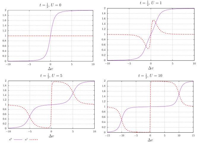
Figure 1: Variation of the ground- $n^{0}$ and first-excited-state $n^{1}$ densities with the local potential $\Delta v$ in the Hubbard dimer for various $U$ values.

where $\Phi_{1}^{KS}(\Delta v)$ is the first singlet (two-electron) excited state of $\hat{\mathcal{H}}^{KS}\left(\Delta v\right)$. Therefore, the density (i.e. the occupation of site 0) in the non-interacting first excited state is equal to 1 for any $t$ and $\Delta v$ values, as illustrated in the top left-hand panel of Fig. 1. Consequently, a density $n$ will be ensemble non-interacting representable in this context if it can be written as $n=(1-w)n^{0}+w$ where the non-interacting ground-state density $n^{0}$ varies in the range $0\leq n^{0}\leq 2$ (see the top left-hand panel of Fig. 1), thus leading to the non-interacting representability condition

$$w\leq n\leq 2-w,$$ (54)

or, equivalently,

$$|n-1|\leq 1-w.$$ (55)

For such densities, the maximizing KS potential in Eq. (47) equals

$$\Delta v^{KS,w}(n)=\frac{2(n-1)t}{\sqrt{(1-w)^{2}-(1-n)^{2}}},$$ (56)

and, consequently, the ensemble non-interacting kinetic energy functional can be expressed analytically as follows,

$$T_{s}^{w}(n)=-2t\sqrt{(1-w)^{2}-(1-n)^{2}}.$$ (57)

The ensemble correlation energy, which is the key quantity studied in this work, is defined as follows,

$$E^{w}_{c}(n)=F^{w}(n)-T_{s}^{w}(n)-E_{H}(n)-E^{w}_{x}(n),$$ (58)

where the Hartree energy equals Smith et al. (2016)

$$E_{H}(n) = \dfrac{U}{2}\Big{(}n^{2}_{0}+n_{1}^{2}\Big{)}$$ (59)

$$= U\Big{(}1+(1-n)^{2}\Big{)}.$$

Note that the latter expression is simply obtained from the conventional one in Eq. (24) by substituting a Dirac-delta interaction with strength $U$ for the regular two-electron repulsion,

$$\dfrac{1}{|{\bf r}-{\bf r}^{\prime}|}\rightarrow U\delta({\bf r}-{\bf r}^{\prime}),$$ (60)

and by summing over sites rather than integrating over the (continuous) real space. The exact ensemble exchange energy in Eq. (30) becomes in this context

$$E^{w}_{x}(n) = (1-w)\langle\Phi^{KS,w}_{0}(n)\rvert\hat{U}\lvert\Phi^{KS,w}_{0}(n)\rangle$$ (61)

$$+w\langle\Phi^{KS,w}_{1}(n)\rvert\hat{U}\lvert\Phi^{KS,w}_{1}(n)\rangle-E_{H}(n),$$

thus leading, according to the Appendix, to the analytical expression

$$E^{w}_{x}(n) = \dfrac{U}{2}\left[1+w-\dfrac{(3w-1)(1-n)^{2}}{(1-w)^{2}}\right]-E_{H}(n),$$ (62)

$$= E^{w=0}_{x}(n)+\dfrac{Uw}{2}\left[1-\dfrac{(1-n)^{2}(1+w)}{(1-w)^{2}}\right],$$

where

$$E^{w=0}_{x}(n)=-E_{H}(n)/2$$ (63)

is the ground-state exchange energy for two unpolarized electrons. Note that the exchange contribution to the GACE integrand (see Eq. (38)) will therefore have a simple analytical expression,

$$\Delta^{w}_{x}(n) = \dfrac{\partial E^{w}_{x}(n)}{\partial w}$$ (64)

$$= \dfrac{U}{2}\left[1-\dfrac{(1-n)^{2}(1+3w)}{(1-w)^{3}}\right].$$

Finally, the maximizing potential $\Delta v^{w}(n)$ in Eq. (46) which reproduces the ensemble density $n$ fulfills, according to the inverse Legendre–Fenchel transform,

$$(1-w)E_{0}(\Delta v^{w}(n))+wE_{1}(\Delta v^{w}(n))$$

$$=\min_{\nu}\Big{\{}F^{w}(\nu)-\Delta v^{w}(n)\times(\nu-1)\Big{\}},$$ (65)

where the minimizing density is $n$. Therefore,

$$\Delta v^{w}(n)=\dfrac{\partial F^{w}(n)}{\partial n},$$ (66)

and, since (see Eqs. (56) and (57))

$$\Delta v^{KS,w}(n)=\partial T_{s}^{w}(n)/\partial n,$$ (67)

the ensemble Hartree-$xc$ potential reads

$$\Delta v_{Hxc}^{w}(n) = \Delta v^{KS,w}(n)-\Delta v^{w}(n)$$ (68)

$$= -\dfrac{\partial E^{w}_{Hxc}(n)}{\partial n}.$$

As a result, the ensemble correlation potential can be calculated exactly as follows,

$$\Delta v_{c}^{w}(n) = \Delta v^{KS,w}(n)-\Delta v^{w}(n)$$ (69)

$$-\Delta v_{H}(n)-\Delta v_{x}^{w}(n),$$

where all contributions but $\Delta v^{w}(n)$ have an analytical expression. The Hartree potential equals $\Delta v_{H}(n)=-\partial E_{H}(n)/\partial n=2U(1-n)$ and, according to Eq. (62), the ensemble exchange potential reads

$$\Delta v_{x}^{w}(n) = -\dfrac{\partial E^{w}_{x}(n)}{\partial n}$$ (70)

$$= U(n-1)\left[1+\dfrac{w(1+w)}{(1-w)^{2}}\right]$$

$$= \Delta v_{x}^{w=0}(n)\left[1+\dfrac{w(1+w)}{(1-w)^{2}}\right].$$

Note the unexpected minus sign on the right-hand side of Eq. (68). It originates from the definition of the potential difference (see Eq. (44)) and the choice of $n_{0}=n$ (occupation of site 0) as variable, the occupation of site 1 being $n_{1}=2-n$. Therefore, $E^{w}_{Hxc}(n)$ can be rewritten as $E^{w}_{Hxc}[n,2-n]$ and

$$\Delta v^{w}_{Hxc}(n) = \left.\frac{\partial E^{w}_{Hxc}[n_{0},n_{1}]}{\partial n_{1}}\right|_{n_{0}=n,n_{1}=2-n}$$ (71)

$$-\left.\frac{\partial E^{w}_{Hxc}[n_{0},n_{1}]}{\partial n_{0}}\right|_{n_{0}=n,n_{1}=2-n}$$

$$= -\frac{\partial E^{w}_{Hxc}[n,2-n]}{\partial n}=-\frac{\partial E^{w}_{Hxc}(n)}{\partial n}.$$

Note finally that, as readily seen in Eq. (70), the ensemble $x$ potential can be expressed in terms of the ground-state $x$ potential ($w=0$) and the ensemble weight. This simple relation, which is transferable to ab initio Hamiltonians, could be used for developing ”true” approximate weight-dependent density-functional $x$ potentials.

IV Exact results

IV.1 Interacting ensemble density and derivative discontinuity

In the rest of the paper, the hopping parameter is set to $t=1/2$. For clarity, we shall refer to the local potential in the physical (fully-interacting) Hubbard Hamiltonian as $\Delta v_{ext}$. This potential is the analog of the nuclear-electron attraction potential in the ab initio Hamiltonian. The corresponding ensemble density is the weighted sum of the ground- $n_{\Delta v_{ext}}^{0}$ and excited-state $n_{\Delta v_{ext}}^{1}$ occupations of site 0,

$$n^{w}=(1-w)n^{0}_{\Delta v_{ext}}+wn^{1}_{\Delta v_{ext}},$$ (72)

where, according to the Hellmann–Feynman theorem,

$$n_{\Delta v_{ext}}^{i}=1-\left.\dfrac{\partial E_{i}(\Delta v)}{\partial\Delta v}\right|_{\Delta v_{ext}}.$$ (73)

Note that the first-order derivative of the energies with respect to $\Delta v$ can be simply expressed in terms of the energies (see Eq. (124)) and that, for a fixed $\Delta v_{ext}$ value, the ensemble density varies linearly with $w$. Ground- and excited-state densities are shown in Fig. 1. For an arbitrary potential value $\Delta v_{ext}=\Delta v$, in the weakly correlated regime ($0<U<<\Delta v$), site occupations are close to 2 or 0 in the ground state and they become equal to 1 in the first excited state. Therefore, in this case, the model describes a charge transfer excitation. On the other hand, in the strongly correlated regime ($U>>\Delta v$), the ground-state density will be close to 1 (symmetric case). When $U$ is large, small changes in $\Delta v$ around $\Delta v=0$ cause large changes in the excited-state density. As clearly seen from the Hamiltonian expression in Eq. (43), when $U\rightarrow+\infty$, site 0 ”gains” an electron when the lowest (singlet) transition occurs if $\Delta v\rightarrow 0^{+}$ whereas, if $\Delta v\rightarrow 0^{-}$, it ”loses” an electron. This explains why the excited-state density curves approach a discontinuous limit at $\Delta v=0$ when $U\rightarrow+\infty$. Let us stress that, for large but finite $U$ values, the latter density will vary rapidly and continuously from 0 to 2 in the vicinity of $\Delta v=0$ while the ground-state density remains close to 1. This observation will enable us to interpret the GACE integrand in the following.

Turning to the calculation of the DD (see Eq. (25)), the latter can be obtained in two ways, either by taking the difference between the physical $\omega=E_{1}(\Delta v_{ext})-E_{0}(\Delta v_{ext})$ and KS

$$\omega^{KS,w}=\varepsilon_{L}\Big{(}\Delta v^{KS,w}(n^{w})\Big{)}-\varepsilon_{H}\Big{(}\Delta v^{KS,w}(n^{w})\Big{)}$$ (74)

excitation energies, which gives

$$\Delta^{w}_{xc} = \omega-\omega^{KS,w},$$ (75)

or by differentiation,

$$\Delta^{w}_{xc} = \left.\dfrac{\partial E^{\xi}_{xc}(n^{w})}{\partial\xi}\right|_{\xi=w}.$$ (76)

In the former case, we obtain from Eqs. (49), (50), and (56) the analytical expression

$$\Delta^{w}_{xc} = E_{1}(\Delta v_{ext})-E_{0}(\Delta v_{ext})$$ (77)

$$-\dfrac{2t(1-w)}{\sqrt{(1-w)^{2}-(1-n^{w})^{2}}}.$$

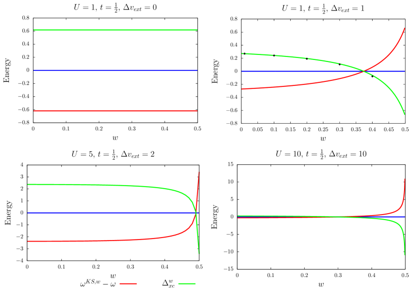
Figure 2: Derivative discontinuity obtained for the Hubbard dimer with different $\Delta v_{ext}$ and $U$ values. Results obtained by numerical differentiation are shown for $\Delta v_{ext}=1$ and $U=1$ (see the black dots on the right-hand top panel). See text for further details.

Regarding Eq. (76), the $\xi$-dependent ensemble $xc$ energy $E^{\xi}_{xc}(n^{w})$ must be determined numerically by means of a Legendre–Fenchel transform calculation (see Eqs. (46) and (58)) and its derivative at $\xi=w$ is then obtained by finite difference. As illustrated in the right-hand top panel of Fig. 2, the two expressions are indeed equivalent. In the symmetric Hubbard dimer ($\Delta v_{ext}=0$), it is clear from Eq. (77) that the DD is weight-independent, since $n^{w}=1$, and it is equal to $[U-4t+\sqrt{U^{2}+16t^{2}}]/2$. In this particular case, the ground and first-excited states actually belong to different symmetries. In the asymmetric case, various patterns are obtained (see Fig. 2). Interestingly, the ”fish picture” obtained by Yang et al. Yang et al. (2014) for the helium atom is qualitatively reproduced by the Hubbard dimer model when $\Delta v_{ext}=U=1$, except in the small-$w$ region where a sharp change in the DD (with positive slope) is observed for the helium atom. This feature does not occur in the two-site model. From the analytical expression,

$$\dfrac{\partial\Delta^{w}_{xc}}{\partial w}=\dfrac{2t(1-n^{w})(n^{1}-1)}{\left[(1-w)^{2}-(1-n^{w})^{2}\right]^{3/2}},$$ (78)

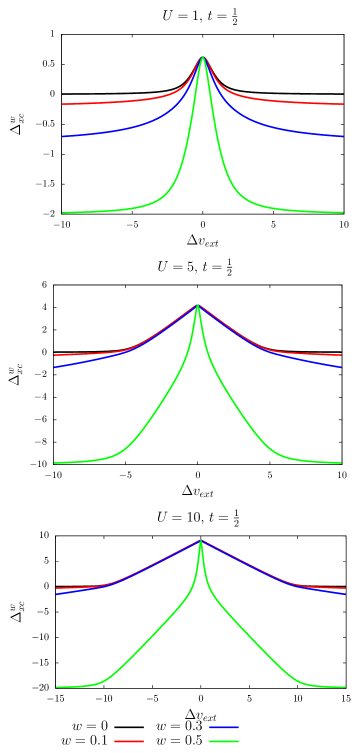
Figure 3: Derivative discontinuity plotted as a function of $\Delta v_{ext}$ for various $w$ and $U$ values.

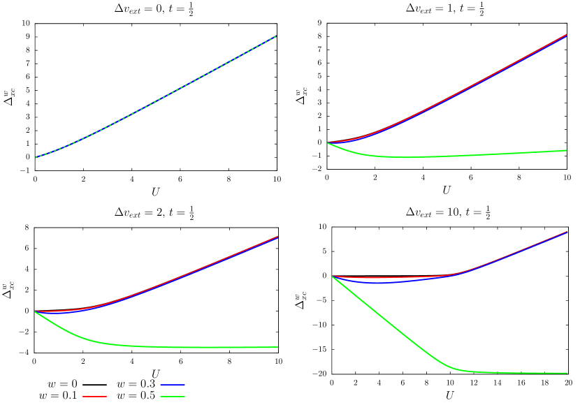
Figure 4: Derivative discontinuity plotted as a function of $U$ for various $w$ and $\Delta v_{ext}$ values.

and Fig. 1, it becomes clear that, in the Hubbard dimer, the DD will systematically decrease with $w$. Variations in $\Delta v_{ext}$ and $U$ for various weights are shown in Figs. 3 and 4, respectively. When $\Delta v_{ext}>>U$, $n^{w}$ is close to $2-w$ (according to Fig. 1) and, since the on-site repulsion becomes a perturbation, the DD can be well reproduced by the exchange-only contribution. Thus, according to Eq. (64), we obtain

$$\Delta^{w}_{xc}\rightarrow\Delta^{w}_{x}(n^{w})\approx-\dfrac{2Uw}{(1-w)}.$$ (79)

As readily seen in Eq. (79), the DD is close to zero for small weights and, when $w=1/2$, it equals $-2U$, which is in agreement with both Figs. 3 and 4. On the other hand, when $t<<\Delta v_{ext}<<U$, the physical energies are expanded as follows, according to Eq. (116),

$$E_{0}(\Delta v_{ext})/U = \dfrac{4}{(\Delta v_{ext}/U)^{2}-1}(t/U)^{2}+\mathcal{O}\left((t/U)^{3}\right)$$

$$E_{1}(\Delta v_{ext})/U = 1-(\Delta v_{ext}/U)+\dfrac{2}{1-(\Delta v_{ext}/U)}(t/U)^{2}$$ (80)

$$+\mathcal{O}\left((t/U)^{3}\right),$$

thus leading to the following expansions for the derivatives,

$$\dfrac{\partial E_{0}(\Delta v_{ext})}{\partial\Delta v_{ext}} = -\dfrac{8(\Delta v_{ext}/U)}{\left[(\Delta v_{ext}/U)^{2}-1\right]^{2}}(t/U)^{2}+\mathcal{O}\left((t/U)^{3}\right)$$

$$\dfrac{\partial E_{1}(\Delta v_{ext})}{\partial\Delta v_{ext}} = -1+\dfrac{2}{\left[1-(\Delta v_{ext}/U)\right]^{2}}(t/U)^{2}$$ (81)

$$+\mathcal{O}\left((t/U)^{3}\right),$$

and, according to Eqs. (72) and (73), to the following expansion for the ensemble density,

$$n^{w}=1+w$$

$$+\dfrac{2(t/U)^{2}}{\left[1-(\Delta v_{ext}/U)\right]^{2}}\Bigg{[}\dfrac{4(1-w)(\Delta v_{ext}/U)}{\left[1+(\Delta v_{ext}/U)\right]^{2}}-w\Bigg{]}$$

$$+\mathcal{O}\left((t/U)^{3}\right).$$ (82)

As readily seen in Eq. (IV.1), the ensemble density is close to 1 in the small-$w$ region. Consequently, according to Eqs. (77) and (IV.1), the DD varies as $U-\Delta v_{ext}$, which is in agreement with the $U=10$ panel of Fig. 3 and the $\Delta v_{ext}=10$ panel of Fig. 4. On the other hand, when $w=1/2$, it comes from Eq. (IV.1),

$$\dfrac{1}{4}-\big{(}1-n^{w=1/2}\big{)}^{2} = \dfrac{(t/U)^{2}}{\left[1+(\Delta v_{ext}/U)\right]^{2}}$$ (83)

$$+\mathcal{O}\left((t/U)^{3}\right),$$

thus leading to the following expansion for the equiensemble DD,

$$\Delta^{w=1/2}_{xc}/U = -2(\Delta v_{ext}/U)+\mathcal{O}(t/U).$$ (84)

The latter expansion matches the behavior observed in the $U=5$ and $U=10$ panels of Fig. 3 as well as $\Delta v_{ext}=2$ and $\Delta v_{ext}=10$ panels of Fig. 4, when $t<<\Delta v_{ext}<<U$. Note finally that, in the $U=10$ panel of Fig. 3, the equiensemble DD is highly sensitive to changes in $\Delta v_{ext}$ around $\Delta v_{ext}=0$ when $U>>t$. In the latter case, the ground-state density remains close to 1 (symmetric dimer), as shown in Fig. 1, and the DD becomes

$$\Delta^{w}_{xc} \rightarrow \dfrac{1}{2}\left[U+\sqrt{U^{2}+16t^{2}}\right]$$ (85)

$$-\dfrac{2t(1-w)}{\sqrt{1-2w+n^{1}_{\Delta v_{ext}}(2-n^{1}_{\Delta v_{ext}})w^{2}}},$$

which is almost constant in the small-$w$ region. When $w=1/2$, the second term on the right-hand side of Eq. (85) becomes $-2t/\sqrt{n^{1}_{\Delta v_{ext}}(2-n^{1}_{\Delta v_{ext}})}$, which decreases rapidly with $\Delta v_{ext}$ as the excited-state density approaches (also rapidly) 2.

Let us finally focus on the weight $w_{xc}$ for which the DD vanishes:

$$\Delta^{w_{xc}}_{xc}=\displaystyle\left.\frac{\partial E^{w}_{xc}(n^{w_{xc}})}{\partial w}\right|_{w=w_{xc}}=0.$$ (86)

For that particular weight, which should of course be used in both KS and physical systems, the (weight-dependent) KS HOMO-LUMO gap is equal to the exact physical (weight-independent) excitation energy, which is remarkable. Note that $w_{xc}$, if it exists, would be fully determined, in practice, from the ”universal” ensemble $xc$ functional. Indeed, for a given local potential $\Delta v_{ext}$, the ensemble density $n^{w}$ (see Eq. (72)) can be obtained by solving two self-consistent KS equations. One with $w=0$ (which gives the ground-state density $n_{\Delta v_{ext}}^{0}$) and a second one with $w=1/2$. In the latter case,

$$n^{w=1/2}=(n_{\Delta v_{ext}}^{0}+n_{\Delta v_{ext}}^{1})/2,$$ (87)

thus leading to $n_{\Delta v_{ext}}^{1}=2n^{w=1/2}-n_{\Delta v_{ext}}^{0}$. The value of $w_{xc}$ would then be obtained from Eq. (86). Solving the ensemble KS equations with the weight $w_{xc}$ would lead to a KS gap which is, in this particular case, the physical optical one. Note that, even though the DD equals zero in this case, it is necessary to know the weight dependence of the ensemble $xc$ functional in order to determine $w_{xc}$. Despite the simplicity of the Hubbard dimer model, $E^{w}_{xc}(n)$ cannot (like in the ground-state case Carrascal et al. (2015)) be expressed analytically in terms of $n$ and $w$. The exact value of $w_{xc}$ has been simply determined from Eq. (77), where the exact physical excitation energy $\omega$ is known, thus leading to the second-order polynomial equation,

$$w_{xc}^{2}\Big{[}\omega^{2}-\omega^{2}\left(n_{\Delta v_{ext}}^{1}-n_{\Delta v_{ext}}^{0}\right)^{2}-4t^{2}\Big{]}$$

$$+2w_{xc}\Big{[}\omega^{2}\left(n_{\Delta v_{ext}}^{0}-n_{\Delta v_{ext}}^{1}\right)\left(n_{\Delta v_{ext}}^{0}-1\right)$$

$$-\omega^{2}+4t^{2}\Big{]}+\omega^{2}n_{\Delta v_{ext}}^{0}(2-n_{\Delta v_{ext}}^{0})-4t^{2}=0.$$ (88)

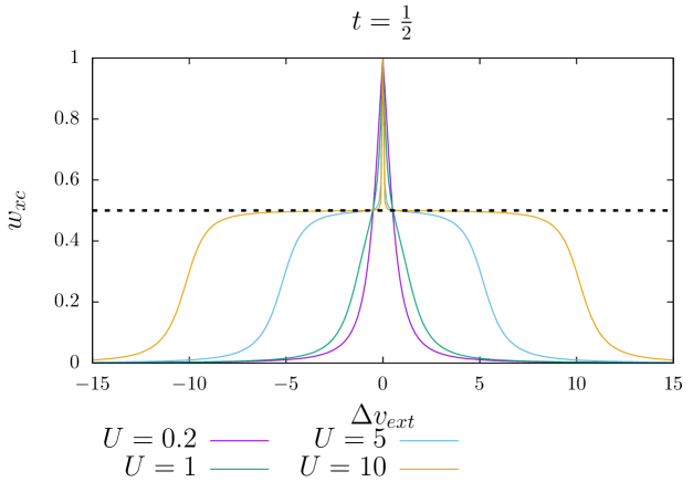
Figure 5: Solution of Eq. (IV.1) plotted with respect to the potential $\Delta v_{ext}$ for different $U$ values. Physical values should be lower than 1/2 (i.e. below the dashed line).

Physical solutions should be in the range $0\leq w_{xc}\leq 1/2$. Results are shown in Fig. 5. In the symmetric Hubbard dimer, the solution becomes $w_{xc}=1$, which is unphysical. This is in agreement with the fact that, in this case, the DD is constant and strictly positive. This is also the reason why no physical values are obtained for $w_{xc}$ in the vicinity of $\Delta v_{ext}=0$. Note finally that $w_{xc}$ is quite sensitive to changes in $\Delta v_{ext}$ around $\Delta v_{ext}=U$ in both weak and strong correlation regimes. This indicates that $w_{xc}$ strongly depends on the system under study.

IV.2 Construction and analysis of the GACE

The general GACE integrand expression in Eq. (39) can, in the case of the Hubbard dimer, be simplified as follows,

$$\Delta^{\xi}_{xc}(n) = E_{1}\Big{(}\Delta v^{\xi}(n)\Big{)}-E_{0}\Big{(}\Delta v^{\xi}(n)\Big{)}$$ (89)

$$-\dfrac{2t(1-\xi)}{\sqrt{(1-\xi)^{2}-(1-n)^{2}}},$$

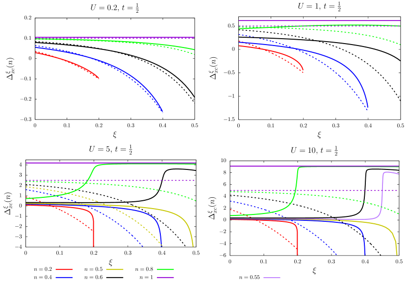
Figure 6: Variation of the exchange-correlation GACE integrand with the ensemble weight $\xi$ for various $U$ values and densities. Comparison is made with the exact exchange-only contribution $\Delta^{\xi}_{x}(n)$ (dashed lines).

where the local potential $\Delta v^{\xi}(n)$ can be computed exactly by means of the Legendre–Fenchel transform in Eq. (46). Results are shown in Fig. 6. Note that, for a fixed density $n$, the non-interacting $v$-representability condition for an ensemble weight $\xi$ (see Eq. (54)) reads

$$0\leq\xi\leq 1-|n-1|.$$ (90)

In the symmetric case ($n=1$), the weight-independent value $[U-4t+\sqrt{U^{2}+16t^{2}}]/2$ is recovered. In the weakly correlated regime ($U=0.2$), the analytical exact exchange expression for the GACE integrand (see Eq. (64)) reproduces very well the total $xc$ one, as expected. When $0\leq n\leq 0.5$, the integrand at $\xi=n$ is therefore well approximated by $\Delta^{\xi=n}_{x}(n)=2Un/(n-1)$. Note also that, away from the symmetric case, the exchange integrand curve crosses over the $xc$ one so that, after integration over the ensemble weight, the ensemble correlation energy remains negligible. In other words, integrals of the exchange and $xc$ integrands are expected to be very similar (i.e. second order in $U$), which explains why the curves have to cross when, in the large-$\xi$ region, the two integrands differ substantially.

Let us now focus on the stronger correlation regimes. For the large $U=5$ and $U=10$ values, we can see plateaus for the considered $n=0.6$ and $n=0.8$ densities in the range $1-n\leq\xi\leq 1/2$, thus leading to discontinuities in the GACE integrand when $U/t\rightarrow+\infty$. As readily seen in Eq. (89), these discontinuities are induced by the $\xi$-dependent fully interacting excitation energy (first term on the right-hand side). As illustrated in Fig. 1, when $U$ is large, the density of the ground state is close to 1 in the vicinity of the symmetric potential ($\Delta v=0$) while the density of the excited state is highly sensitive to small changes in the potential. The reason is that, in the $U/t\rightarrow+\infty$ limit, states with a doubly-occupied site are degenerate (with energy $U$) when $\Delta v=0$. The degeneracy is lifted when $\Delta v$ is not strictly zero. For finite but large $U/t$ values, the first-excited state density will vary continuously and rapidly from 0 to 2 in the vicinity of $\Delta v=0$. Therefore, within the GACE, the fully-interacting ensemble density reads $n=(1-\xi)+\xi n^{1,\xi}$ with the condition $0\leq n^{1,\xi}\leq 2$, thus leading to

$$n^{1,\xi}=1+\dfrac{n-1}{\xi},$$ (91)

and $|1-n|\leq\xi\leq 1/2$. The latter range describes exactly the plateaus observed in the $U=10$ panel of Fig. 6. In this case, the GACE potential in the physical system is almost symmetric, thus leading to the following approximate value for the plateau,

$$\Delta^{\xi}_{xc}(n) \approx \dfrac{1}{2}(U+\sqrt{U^{2}+16t^{2}})$$ (92)

$$-\dfrac{2t(1-\xi)}{\sqrt{(1-\xi)^{2}-(1-n)^{2}}}.$$

This expression will be used in the following section for analyzing the ensemble $xc$ energy and potential. Note that the $\xi$-dependent part of the integrand (second term on the right-hand side of Eq. (92)) decreases with $\xi$ over the range $(1-n)\leq\xi\leq 1/2$ with $1/2\leq n\leq 1$, as clearly seen in the $U=5$ and $U=10$ panels of Fig. 6. The $\xi$-dependence disappears as $U/t$ increases.

We also in Fig. 6 that, outside the plateaus, the GACE integrand becomes relatively small as $U$ increases. This can be interpreted as follows. In the $U/t\rightarrow+\infty$ limit, when $\Delta v=\pm U$, the ground (with singly occupied sites) and first-excited (with a doubly occupied site) states become degenerate with energy 0. If we consider, for example, an infinitesimal positive deviation from $-U$ in the potential, sites will be singly occupied in the ground state and site 0 will be empty in the first excited state. It would be the opposite if the deviation were negative, thus leading to discontinuites in the ground- and excited-state densities at $\Delta v=\pm U$, as expected from the $U=10$ panel of Fig. 1. For large but finite $U/t$ values, the ground-state density will vary continuously from 0 to 1 around $\Delta v=-U$ while the first-excited-state density varies from 1 to 0. The first excitation is a charge transfer. It means that, in this case, the fully-interacting ensemble density with weight $\xi$ can be written as $n=(1-\xi)n^{0,\xi}+\xi n^{1,\xi}$ with $n^{0,\xi}+n^{1,\xi}=1$, thus leading to

$$n^{0,\xi}-1=\dfrac{n-1+\xi}{1-2\xi}.$$ (93)

Therefore, for a given density $n$, the condition $0\leq n^{0,\xi}\leq 1$ can be rewritten as $\xi\leq 1-n$ in addition to the non-interacting $v$-representability condition in Eq. (90). Note that, around $\Delta v=U$, this condition becomes $0\leq\xi\leq n-1$. In summary, for a fixed density $n$, the range of ensemble weights $0\leq\xi\leq|1-n|$ can be described in the vicinity of $\Delta v=\pm U$. This range corresponds to situations where no plateau is observed in the GACE integrand. Since, according to Eq. (116), the ground- and first-excited-state energies at $\Delta v=\pm U$ can be expanded as follows,

$$E_{0}(\pm U)/U = -\sqrt{2}t/U+\mathcal{O}(t^{2}/U^{2}),$$

$$E_{1}(\pm U)/U = \sqrt{2}t/U+\mathcal{O}(t^{2}/U^{2}),$$ (94)

we conclude that, when $0\leq\xi\leq|1-n|$ and $U$ is large, an approximate GACE integrand expression is

$$\Delta^{\xi}_{xc}(n) \approx 2\sqrt{2}t-\dfrac{2t(1-\xi)}{\sqrt{(1-\xi)^{2}-(1-n)^{2}}}.$$ (95)

Note that, for an ensemble non-interacting representable density $n$ such that $n<1$, the condition $\xi\leq n$ must be fulfilled, according to Eq. (90). If, in addition, $n\leq 1-n$ (i.e. $n\leq 1/2$), then the GACE integrand is expected to diverge in the strongly correlated limit when $\xi\rightarrow n$, which is exactly what is observed in the $U=10$ panel of Fig. 6.

IV.3 Weight-dependent exchange-correlation energy and potential

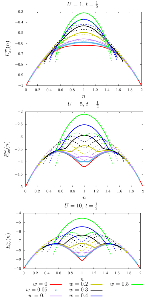
Figure 7: Exact ensemble density-functional exchange-correlation energies for various $U$ and $w$ values. The mixed ensemble exchange/ ground-state correlation energy $E_{x}^{w}(n)+E_{c}^{w=0}(n)$ is shown (dashed lines) for analysis purposes.

Exact ensemble $xc$ density-functional energies are shown in Fig. 7. As discussed just after Eq. (90), in the strictly symmetric case ($n=1$), the GACE integrand is weight-independent, thus leading to an ensemble $xc$ energy with weight $w$ that deviates from its ground state value by $w[U-4t+\sqrt{U^{2}+16t^{2}}]/2$. Therefore this deviation increases with the weight, as clearly illustrated in Fig. 7. In the weakly correlated regime, the deviation from the ground-state functional is essentially driven by the exchange contribution, as expected. For $U=1$, the deviation induced by the correlation energy becomes significant when approaching the equiensemble case. On the other hand, in stronger correlation regimes ($U=5$ and 10), the weight-dependence of the ensemble correlation energy becomes crucial even for relatively small ensemble weights. The bumps observed at $n=1$ are a pure ensemble correlation effect. In the light of Sec. IV.2, we can conclude that these bumps, which correspond to the largest deviation from the ground-state xc functional, are induced by the plateaus in the GACE integrand which are defined in the range $|1-n|\leq\xi$. Outside this range, the integrand is given by Eq. (95). Consequently, for given ensemble weight $w$ and density $n$ such that $w\leq|1-n|$, which leads to

$$w\leq n\leq 1-w\;\;\;{\rm or}\;\;\;1+w\leq n\leq 2-w,$$ (96)

when considering, in addition, the $v$-representability condition in Eq. (54), the ensemble $xc$ energy (whose deviation from its ground-state value is obtained by integration from 0 to $w$) can be approximated as follows,

$$E^{w}_{xc}(n) \approx E_{xc}(n)+2t\Bigg{(}\sqrt{2}w+\sqrt{(1-w)^{2}-(1-n)^{2}}$$ (97)

$$-\sqrt{1-(1-n)^{2}}\Bigg{)},$$

which approaches the ground-state $xc$ energy when $U/t\rightarrow+\infty$. For finite but large $U/t$ values, we obtain at the border of the $v$-representable density domain (i.e. for $n=w$ or $n=2-w$),

$$E^{w}_{xc}(w) \approx E_{xc}(w)+\dfrac{2tw(3w-2)}{\sqrt{2}w+\sqrt{1-(1-w)^{2}}},$$ (98)

where the second term on the right-hand side is negative, and $E^{w}_{xc}(2-w)=E^{w}_{xc}(w)$ because of the hole-particle symmetry. From these derivations, we can match the behavior of the exact curves in Fig. 7 for densities that fulfill Eq. (96). Note finally that, for such densities, the ensemble $xc$ potential can be approximated as follows, according to Eq. (68) and (97),

$$\Delta v^{w}_{xc}(n)=-\dfrac{\partial E^{w}_{xc}(n)}{\partial n}$$

$$\approx\Delta v_{xc}(n)+2t(n-1)\Bigg{[}\dfrac{1}{\sqrt{(1-w)^{2}-(1-n)^{2}}}$$

$$-\dfrac{1}{\sqrt{1-(1-n)^{2}}}\Bigg{]}.$$ (99)

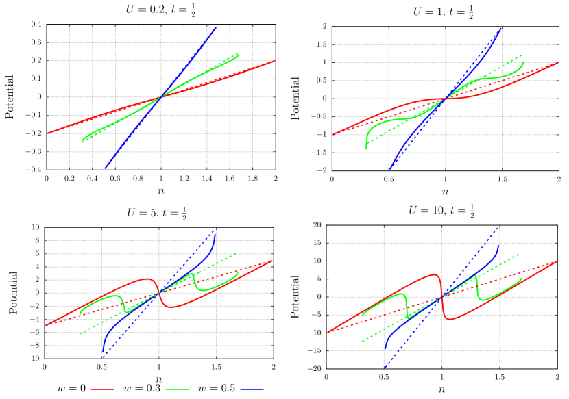
Figure 8: Exact ensemble exchange-correlation potential for various $U$ and $w$ values. The exact ensemble exchange potential (dashed lines) is shown for analysis purposes.

As expected and confirmed by the exact results of Fig. 8, the ensemble $xc$ potential becomes the ground-state one in the density domains of Eq. (96) when $U/t\rightarrow+\infty$.

Let us now focus on the complementary range $w\geq|1-n|$ or, equivalently,

$$1-w\leq n\leq 1+w.$$ (100)

In this case, the ensemble $xc$ energy is obtained by integrating over $[0,|1-n|]$ and $[|1-n|,w]$ weight domains, thus leading to the following approximate expression, according to Eqs. (92) and (95),

$$E^{w}_{xc}(n)\approx E_{xc}(n)+\dfrac{1}{2}\Big{(}U+\sqrt{U^{2}+16t^{2}}\Big{)}(w-|1-n|)$$

$$+2t\Bigg{(}\sqrt{2}|1-n|+\sqrt{(1-w)^{2}-(1-n)^{2}}$$

$$-\sqrt{1-(1-n)^{2}}\Bigg{)}.$$ (101)

Turning to the ensemble $xc$ potential, it comes from Eq. (IV.3) that

$$\Delta v^{w}_{xc}(n)\approx\Delta v_{xc}(n)$$

$$+ \Bigg{[}2t\sqrt{2}-\dfrac{1}{2}\Big{(}U+\sqrt{U^{2}+16t^{2}}\Big{)}\Bigg{]}\dfrac{|1-n|}{1-n}$$ (102)

$$+2t(n-1)\Bigg{[}\dfrac{1}{\sqrt{(1-w)^{2}-(1-n)^{2}}}$$

$$-\dfrac{1}{\sqrt{1-(1-n)^{2}}}\Bigg{]}.$$

Since, in the $U/t\rightarrow+\infty$ limit, the ground-state $xc$ potential becomes discontinuous at $n=1$ and equal to Senjean et al. (2016)

$$\Delta v_{xc}(n)\rightarrow 2U(n-1)+U\dfrac{|1-n|}{1-n},$$ (103)

we conclude from Eq. (IV.3) that, in the strongly correlated limit, the ensemble $xc$ potential becomes, in the range $1-w\leq n\leq 1+w$,

$$\Delta v^{w}_{xc}(n)\rightarrow 2U(n-1),$$ (104)

where, as readily seen, the ground-state discontinuity at $n=1$ has been removed. This is in perfect agreement with the $U=10$ panel of Fig. 8. Note that, even though the exact exchange potential varies also linearly with $n$, its slope is weight-dependent (see Eq. (70)) and equals the expected $2U$ value only when $w=1/3$, as illustrated in Fig. 8. In other words, both exchange and correlation contributions are important in the vicinity of $n$=1. Strong correlation effects become even more visible at the borders of the bumps in the $xc$ ensemble energy, namely $n=1\pm w$. Indeed, at these particular densities, the ensemble $xc$ potential exhibits discontinuities that are, according to Eqs. (IV.3) and (IV.3), equal to

$$\left.\Delta v^{w}_{xc}(n)\right|_{n=(1\pm w)^{+}}-\left.\Delta v^{w}_{xc}(n)\right|_{n=(1\pm w)^{-}}$$

$$\approx 2t\sqrt{2}-\dfrac{1}{2}\Big{(}U+\sqrt{U^{2}+16t^{2}}\Big{)},$$ (105)

which becomes $-U$ when $U/t\rightarrow+\infty$. Let us stress that Eq. (IV.3) holds for $0<w\leq 1/2$. It relies on the continuity of the ground-state $xc$ potential around $n=1\pm w$, which explains why the ground-state case $w=0$ is excluded. Note finally that, in the strongly correlated limit, the ground-state discontinuity at $n=1$ equals, according to Eq. (103),

$$\left.\Delta v_{xc}(n)\right|_{n=1^{+}}-\left.\Delta v_{xc}(n)\right|_{n=1^{-}}=-2U,$$ (106)

which is twice the ensemble discontinuity at $n=1\pm w$, in agreement with the panel $U=10$ of Fig. 8.

V Ground-state density-functional approximations

In practical eDFT calculations, it is common to use (weight-independent) ground-state (GS) $xc$ functionals Senjean et al. (2015); Alam et al. (2016). Such an approximation induces in principle both energy- and density-driven errors. In this paper, we will only discuss the former, which means that approximate ensemble energies are calculated with exact ensemble densities. The exact GS $xc$ functional will be used and the approximation will be referred to as GS$xc$. The analysis of the density-driven errors ($\it i.e.$ the errors induced by the self-consistent calculation of the ensemble density with the GS $xc$ density-functional potential) requires the use an accurate parameterization for the GS correlation functional Carrascal et al. (2015). This is left for future work. For analysis purposes, we also combined the exact (analytical) ensemble exchange functional with the exact GS correlation functional, thus leading to the GS$c$ approximation. In summary, for a given local potential $\Delta v_{ext}$, the following exact

$$E^{w} = T^{w}_{s}(n^{w})+(1-n^{w})\Delta v_{ext}+E_{H}(n^{w})$$ (107)

$$+E^{w}_{xc}(n^{w}),$$

and approximate

$$E_{{\rm GS}xc}^{w} = E^{w}+E^{w=0}_{xc}(n^{w})-E^{w}_{xc}(n^{w}),$$

$$E_{{\rm GS}c}^{w} = E_{{\rm GS}xc}^{w}-E^{w=0}_{x}(n^{w})+E^{w}_{x}(n^{w})$$ (108)

ensemble energies have been computed, where $n^{w}$ is the exact ensemble density. Note that, if Boltzmann weights were used Pastorczak et al. (2013), GS$xc$ would be similar to the zero-temperature approximation (ZTA) of Ref. Smith et al. (2016). A significant difference, though, is that ZTA is using a self-consistent density (thus inducing density-driven errors) while, in GS$xc$, we use the exact ensemble density. The comparison of GS$xc$, GS$c$ and ZTA is left for future work.

The approximate (weight-dependent) GS$xc$ and GS$c$ excitation energies are obtained by differentiation with respect to $w$, thus leading to, according to Eqs. (64), (66), (67) and (70),

$$\omega_{{\rm GS}xc}^{w}=\left.\dfrac{\partial T^{w}_{s}(n)}{\partial w}\right|_{n=n^{w}}+\Bigg{(}\Delta v^{KS,w}(n^{w})$$

$$-\Delta v^{KS,w=0}(n^{w})+\Delta v^{w=0}(n^{w})-\Delta v_{ext}\Bigg{)}\dfrac{\partial n^{w}}{\partial w},$$ (109)

and

$$\omega_{{\rm GS}c}^{w} = \omega_{{\rm GS}xc}^{w}+\Delta^{w}_{x}(n^{w})$$ (110)

$$-\Big{(}\Delta v_{x}^{w}(n^{w})-\Delta v_{x}^{w=0}(n^{w})\Big{)}\dfrac{\partial n^{w}}{\partial w},$$

where, according to Eqs. (57) and (72),

$$\left.\dfrac{\partial T^{w}_{s}(n)}{\partial w}\right|_{n=n^{w}} = \dfrac{2t(1-w)}{\sqrt{(1-w)^{2}-(1-n^{w})^{2}}},$$ (111)

$$\dfrac{\partial n^{w}}{\partial w} = n^{1}_{\Delta v_{ext}}-n^{0}_{\Delta v_{ext}}.$$ (112)

Note finally that, when inserting the ensemble density of the KS system $n^{w}=(1-w)n^{0,w}_{KS}+wn^{1,w}_{KS}$ into the Hartree functional (see the first line of Eq. (59)), we obtain the following decomposition,

$$E_{H}(n^{w})=(1-w)^{2}E_{H}(n^{0,w}_{KS})+w^{2}E_{H}(n^{1,w}_{KS})$$

$$+2Uw(1-w)\Big{[}1+(1-n^{0,w}_{KS})(1-n^{1,w}_{KS})\Big{]},$$ (113)

where the last term on the right-hand side is an (unphysical) interaction contribution to the ensemble energy that ”couples” the ground and first excited states. It is known as ghost-interaction error Gidopoulos et al. (2002) and, since $n^{1,w}_{KS}=1$ (see Eq. (III)), it simply equals $2Uw(1-w)$. This error is removed when employing the exact ensemble exchange functional, as readily seen in Eq. (61). Therefore, GS$c$ is free from ghost interaction errors whereas GS$xc$ is not. In the latter case, only half of the error is actually removed, according to Eq. (63). In order to visualize the impact of the errors induced by the approximate calculation of the exchange energy (which includes the ghost-interaction error), we combined the GS exchange functional with the exact ensemble correlation one, thus leading to the GS$x$ approximate ensemble energy,

$$E_{{\rm GS}x}^{w} = E^{w}+E^{w=0}_{x}(n^{w})-E^{w}_{x}(n^{w})$$ (114)

$$= E^{w}+E_{{\rm GS}xc}^{w}-E_{{\rm GS}c}^{w},$$

and the corresponding derivative,

$$\omega_{{\rm GS}x}^{w}=\omega+\omega_{{\rm GS}xc}^{w}-\omega_{{\rm GS}c}^{w}.$$ (115)

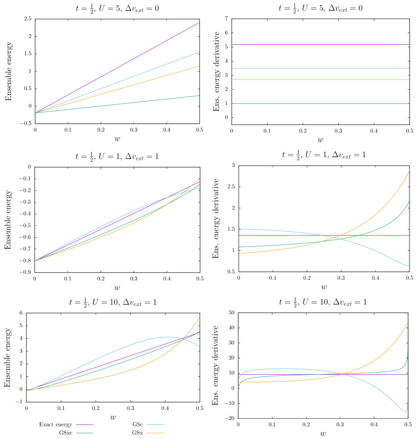
Figure 9: Comparing exact with approximate ensemble energies (left panels) and first-order derivatives (right panels) for various $\Delta v_{ext}$ and $U$ values. See text for further details.

Results are shown in Fig. 9 for various correlation regimes. In the symmetric case ($\Delta v_{ext}=0$), $n^{w}=1$ so that both exact and approximate ensemble energies are linear in $w$ and, as expected from Fig. 7, GS$c$ performs better than GS$xc$. In the asymmetric case ($\Delta v_{ext}=1$), approximate ensemble energies become curved, as expected. For $U=1$, GS$c$ remains more accurate than GS$xc$ (except for the equiensemble). However, in the strongly correlated regime ($U=10$) and for $w\geq 0.1$, the use of the ensemble exact exchange energy in conjunction with the GS correlation functional induces large errors on the ensemble energy. When approaching the equiensemble, the ensemble energy becomes concave. The negative slope in the large-$w$ region leads to negative approximate excitation energies, which is of course unphysical. On the other hand, using both ground-state exchange and correlation functionals provides much better results. This can be rationalized as follows. According to Fig. 1, when $\Delta v_{ext}=1$ and $U=10$, the equiensemble density equals 1.5, which corresponds to the border of the bump in the ensemble $xc$ energy that was discussed previously. Using the $U=10$ panel of Fig. 7, we conclude that GS$c$ underestimates the equiensemble correlation energy significantly while the exact ensemble $xc$ energy is almost identical to the ground-state one. The former is in fact slightly lower than the latter, as expected from Eq. (98) and confirmed by the $U=10$ panel of Fig. 9. Therefore, in this particular case, GS$xc$ is much more accurate than GS$c$. Interestingly, despite large errors in both exchange (which includes the ghost-interaction error) and correlation energies for most weight values, relatively accurate results are obtained through error cancellation. Note finally that, for $\Delta v_{ext}=1$ and $U=10$, GS$xc$ and GS$c$ ensemble energy derivatives increase rapidly when approaching the equiensemble case. This is due to the non-interacting ensemble kinetic energy. Since the ground- and excited-state densities are close to 1 and 2, respectively, $T_{s}^{w}(n^{w})\approx-2t\sqrt{1-2w}$ and ${\rm d}T_{s}^{w}(n^{w})/{\rm d}w\approx 2t/\sqrt{1-2w}$.

VI Conclusion

eDFT is an exact time-independent alternative to TD-DFT for the calculation of neutral excitation energies. Even though the theory has been proposed almost thirty years ago, it is still not standard due to the lack of reliable density-functional approximations for ensembles. In this paper, exact two-state eDFT calculations have been performed for the nontrivial asymmetric two-electron Hubbard dimer. In this system, the density is given by a single number which is the occupation $n$ ($0\leq n\leq 2$) of one of the two sites. An exact analytical expression for the weight-dependent ensemble exchange energy has been derived. Even though the ensemble correlation energy is not analytical, it can be computed exactly, for example, by means of Legendre–Fenchel transforms. Despite its simplicity, this model has shown many features which can be observed in realistic electronic systems. In particular, the derivative discontinuity associated with neutral excitations could be plotted and analyzed in various correlation regimes. It appears that, in many situations, it is possible to find an ensemble weight such that the KS gap equals exactly the optical one.
We have also shown that, in order to connect the ensemble $xc$ functional with weight $w$ ($0\leq w\leq 1/2$) to the ground-state one ($w=0$), a generalized adiabatic connection for ensembles (GACE), where the integration is performed over the ensemble weight rather than the interaction strength, can be constructed exactly for any ensemble-representable density. The GACE formalism was used for analyzing exact ensemble $xc$ energies in the strongly correlated regime. In particular, we could show that in the density domains $w\leq n\leq 1-w$ and $1+w\leq n\leq 2-w$, the ensemble $xc$ energy is well approximated by the ground-state one whereas, in the range $1-w\leq n\leq 1+w$, the ensemble and ground-state $xc$ energies can differ substantially. The difference is actually, in the strongly correlated limit, proportional to $Uw$ when $n=1$. The existence of these three density domains is directly connected to the fact that, in the strongly correlated regime, the well-known discontinuity at $n=1$ in the ground-state $xc$ potential is removed when $w>0$ and it is replaced by two discontinuities, at $n=1-w$ and $n=1+w$, respectively.
Finally, ground-state density-functional approximations have been tested and the associated functional-driven error has been analyzed. Whereas the use of the exact (weight-dependent) ensemble exchange functional in conjunction with the ground-state (weight-independent) correlation functional provides better ensemble energies (than when calculated with the ground-state $xc$ functional) in the strictly symmetric or weakly correlated cases, the combination of both ground-state exchange and correlation functionals provides much better (sometimes almost exact) results away from the small-$w$ region when the correlation is strong. Indeed, in the latter case, the ground-state density is close to 1 and the excitation corresponds to a charge transfer, thus leading to an excited density close to 2 or 0. The resulting ensemble density will therefore be close to $1+w$ or $1-w$. As already mentioned, for $n=1\pm w$, the weight dependence of the ensemble $xc$ functional becomes negligible as $U/t$ increases. This supports the idea that the use of ground-state functionals in practical eDFT calculations is not completely irrelevant. The analysis of density-driven errors is currently in progress. One important conclusion of this work, regarding its extension to ab initio Hamiltonians, is that the calculation of the GACE integrand plays a crucial role in the analysis of exchange-correlation energies of ensembles and, consequently, in the construction of ”true” approximate density functionals for ensembles. The accurate computation of this integrand for small molecular systems would be of high interest in this respect. We hope that the paper will stimulate new developments in eDFT.

*

Appendix A Energies and derivatives

Individual ground- and first-excited-state singlet energies $E_{i}$ ($i=0,1$) are in principle functions of $t$, $U$ and $\Delta v$, and they are solutions of

$$-4t^{2}U+(4t^{2}-U^{2}+\Delta v^{2})E_{i}+2UE_{i}^{2}=E_{i}^{3}.$$ (116)

The exact ground-state energy can be expressed analytically as follows Carrascal et al. (2015),

$$E_{0}(U,\Delta v)=\dfrac{4t}{3}\left(u-w\,{\rm sin}\left(\theta+\dfrac{\pi}{6}\right)\right),$$ (117)

where

$$u=\dfrac{U}{2t},$$ (118)

$$w=\sqrt{3(1+\nu^{2})+u^{2}},$$ (119)

$$\nu=\dfrac{\Delta v}{2t},$$ (120)

and

$${\rm cos}(3\theta)=\left(9(\nu^{2}-1/2)-u^{2}\right)u/w^{3}.$$ (121)

The first-excited-state energy is then obtained by solving a second-order polynomial equation for which analytical solutions can be found Smith et al. (2016).

Differentiating Eq. (116) with respect to $U$ gives

$$\frac{\partial E_{i}}{\partial U}=\frac{4t^{2}+2UE_{i}-2E_{i}^{2}}{4t^{2}-U^{2}+4UE_{i}+\Delta v^{2}-3E_{i}^{2}}.$$ (122)

Since, according to the Hellmann–Feynman theorem,

$$\langle\Phi^{KS,w}_{i}(n)\rvert\hat{U}\lvert\Phi^{KS,w}_{i}(n)\rangle=U\left.\dfrac{\partial E_{i}}{\partial U}\right|_{\Delta v^{KS,w}(n),U=0},$$ (123)

combining Eqs. (49), (52), (56) with Eq. (61) finally leads to the expression in Eq. (62).
Similarly, we obtain the following expression for the derivative of individual energies with respect to the local potential,

$$\dfrac{\partial E_{i}}{\partial\Delta v}=\dfrac{2\Delta vE_{i}}{3E_{i}^{2}-4UE_{i}+U^{2}-4t^{2}-\Delta v^{2}}.$$ (124)

References

- Runge and Gross (1984) E. Runge and E. K. U. Gross, Phys. Rev. Lett. 52, 997 (1984).
- Casida and Huix-Rotllant (2012) M. Casida and M. Huix-Rotllant, Annu. Rev. Phys. Chem. 63, 287 (2012).
- Görling (1999) A. Görling, Phys. Rev. A 59, 3359 (1999).
- Levy and Nagy (1999) M. Levy and A. Nagy, Phys. Rev. Lett. 83, 4361 (1999).
- Gaudoin and Burke (2004) R. Gaudoin and K. Burke, Phys. Rev. Lett. 93, 173001 (2004).
- Ayers and Levy (2009) P. W. Ayers and M. Levy, Phys. Rev. A 80, 012508 (2009).
- Ziegler et al. (2009) T. Ziegler, M. Seth, M. Krykunov, J. Autschbach, and F. Wang, J. Chem. Phys. 130, 154102 (2009).
- Ayers et al. (2012) P. W. Ayers, M. Levy, and A. Nagy, Phys. Rev. A 85, 042518 (2012).
- Krykunov and Ziegler (2013) M. Krykunov and T. Ziegler, J. Chem. Th. Comp. 9, 2761 (2013).
- Theophilou (1979) A. K. Theophilou, J. Phys. C (Solid State Phys.) 12, 5419 (1979).
- Gross et al. (1988a) E. K. U. Gross, L. N. Oliveira, and W. Kohn, Phys. Rev. A 37, 2809 (1988a).
- Gross et al. (1988b) E. K. U. Gross, L. N. Oliveira, and W. Kohn, Phys. Rev. A 37, 2805 (1988b).
- Pastorczak et al. (2013) E. Pastorczak, N. I. Gidopoulos, and K. Pernal, Phys. Rev. A 87, 062501 (2013).
- Gidopoulos et al. (2002) N. I. Gidopoulos, P. G. Papaconstantinou, and E. K. U. Gross, Phys. Rev. Lett. 88, 033003 (2002).
- Pastorczak and Pernal (2014) E. Pastorczak and K. Pernal, J. Chem. Phys. 140, 18A514 (2014).
- Yang et al. (2014) Z.-h. Yang, J. R. Trail, A. Pribram-Jones, K. Burke, R. J. Needs, and C. A. Ullrich, Phys. Rev. A 90, 042501 (2014).
- Borgoo et al. (2015) A. Borgoo, A. M. Teale, and T. Helgaker, AIP Conference Proceedings 1702, 090049 (2015).
- Pribram-Jones et al. (2014) A. Pribram-Jones, Z.-h. Yang, J. R. Trail, K. Burke, R. J. Needs, and C. A. Ullrich, J. Chem. Phys. 140, 18A541 (2014).
- Carrascal et al. (2015) D. J. Carrascal, J. Ferrer, J. C. Smith, and K. Burke, J. Phys. Condens. Matter 27, 393001 (2015).
- Smith et al. (2016) J. C. Smith, A. Pribram-Jones, and K. Burke, Phys. Rev. B 93, 245131 (2016).
- Eschrig (2003) H. Eschrig, The Fundamentals of Density Functional Theory, 2nd ed. (Eagle, Leipzig, 2003) edition am Gutenbergplatz.
- Kutzelnigg (2006) W. Kutzelnigg, J. Mol. Structure: THEOCHEM 768, 163 (2006).
- van Leeuwen (2003) R. van Leeuwen, Adv. Quantum Chem. 43, 25 (2003).
- Lieb (1983) E. H. Lieb, Int. J. Quantum Chem. 24, 243 (1983).
- Franck and Fromager (2014) O. Franck and E. Fromager, Mol. Phys. 112, 1684 (2014).
- Levy (1995) M. Levy, Phys. Rev. A 52, R4313 (1995).
- Stein et al. (2012) T. Stein, J. Autschbach, N. Govind, L. Kronik, and R. Baer, J. Phys. Chem. Lett. 3, 3740 (2012).
- Kraisler and Kronik (2013) E. Kraisler and L. Kronik, Phys. Rev. Lett. 110, 126403 (2013).
- Kraisler and Kronik (2014) E. Kraisler and L. Kronik, J. Chem. Phys. 140, 18A540 (2014).
- Gould and Toulouse (2014) T. Gould and J. Toulouse, Phys. Rev. A 90, 050502 (2014).
- Langreth and Perdew (1975) D. C. Langreth and J. P. Perdew, Solid State Commun. 17, 1425 (1975).
- Gunnarsson and Lundqvist (1976) O. Gunnarsson and B. I. Lundqvist, Phys. Rev. B 13, 4274 (1976).
- Langreth and Perdew (1977) D. C. Langreth and J. P. Perdew, Phys. Rev. B 15, 2884 (1977).
- Savin et al. (2003) A. Savin, F. Colonna, and R. Pollet, Int. J. Quantum Chem. 93, 166 (2003).
- Nagy (1995) A. Nagy, Int. J. Quantum Chem. 56, 225 (1995).
- Senjean et al. (2016) B. Senjean, M. Tsuchiizu, V. Robert, and E. Fromager, Mol. Phys. (2016), http://dx.doi.org/10.1080/00268976.2016.1182224 .
- Chayes et al. (1985) J. Chayes, L. Chayes, and M. B. Ruskai, J. Stat. Phys. 38, 497 (1985).
- Gunnarsson and Schönhammer (1986) O. Gunnarsson and K. Schönhammer, Phys. Rev. Lett. 56, 1968 (1986).
- Schönhammer et al. (1995) K. Schönhammer, O. Gunnarsson, and R. M. Noack, Phys. Rev. B 52, 2504 (1995).
- Capelle and Campo Jr. (2013) K. Capelle and V. L. Campo Jr., Phys. Rep. 528, 91 (2013).
- Senjean et al. (2015) B. Senjean, S. Knecht, H. J. Aa. Jensen, and E. Fromager, Phys. Rev. A 92, 012518 (2015).
- Alam et al. (2016) M. M. Alam, S. Knecht, and E. Fromager, Phys. Rev. A 94, 012511 (2016).
*