Inflation via logarithmic entropy-corrected holographic dark energy model

Abstract

We study the inflation via logarithmic entropy-corrected holographic dark energy LECHDE model with future event horizon, particle horizon and Hubble horizon cut-offs, and compare the results with those of obtained in the study of inflation by holographic dark energy HDE model. In comparison, the spectrum of primordial scalar power spectrum in the LECHDE model becomes redder than the spectrum in HDE model. Moreover, the consistency with the observational data in LECHDE model of inflation, constrains the reheating temperature and Hubble parameter by one parameter of holographic dark energy and two new parameters of logarithmic corrections.
Keywords: Inflation, Holographic dark energy.

I Introduction

The recent cosmological and astrophysical data from Cosmic Microwave Background radiation (CMB), the observations type Ia supernovae and Large Scale Structure (LSS) persuasive express that the universe experiences an accelerated expansion phase Riess . The accelerated expansion phase is derived by a energy component with negative pressure so called dark energy (DE). The most simple candidate for dark energy is the cosmological constant, $\Lambda$. However, the cosmological constant candidate suffers from the fine-tuning and the cosmic coincidence problems copeland ; Swein . Therefore, cosmologists suggested some different models for DE including tachyon, quintessence, phantom, k-essence, chaplygin gas, holographic and new agegraphic models Li1 ; Li2 ; wei ; pad ; setare ; msetare ; MRsetare .

The holographic dark energy model HDE is one of the models of quantum gravity. This model, based on the holographic principle, was proposed in Ref.suss by introducing the following energy density

$$\varrho_{\Lambda}=3c^{2}M_{P}^{2}L^{-2},$$ (1)

where $c$ is a numerical constant to be determined by observational data. $L$ and $M_{P}$ are the cut-off radius and the reduced Planck mass, respectively.

The Bekenstein-Hawking entropy $S_{BH}=\frac{A}{4G}$ which is satisfied on the horizon, plays a fundamental role in the HDE model wald . In fact, $A\sim L^{2}$ is the area of horizon and since the holographic dark energy model is related to the area law of entropy, therefore any correction to the area law of entropy will modify the energy density of the HDE model. One correction to the area law of entropy is the logarithmic correction Maj

$$S_{BH}=\frac{A}{4G}+\tilde{\alpha}\ln(\frac{A}{4G})+\tilde{\beta}.$$ (2)

Here $\tilde{\alpha}$ and $\tilde{\beta}$ are dimensionless constants. The correction terms play a fundamental role in the early time inflation and late-time acceleration of the universe cai . The corresponding modified energy density of the Logarithmic Entropy-Corrected Holographic Dark Energy (LECHDE ) model has expressed by Wei WWi

$$\rho_{\Lambda}=3c^{2}M_{P}^{2}L^{-2}+L^{-4}\Big{[}\alpha\ln(M_{P}^{2}L^{2})+\beta\Big{]},$$ (3)

where $\alpha$ and $\beta$ are dimensionless constants. In Eq. (3), the second and third terms are comparable to the first term when $L$ takes a very small amount. This means that the correction terms are important in early universe and when the universe becomes large, the second and third terms are ignorable and the logarithmic entropy-corrected holographic dark energy model reduces to the ordinary holographic dark energy model. The fractional energy density of LECHDE is given by

$$\Omega_{\Lambda}=\frac{\rho_{\Lambda}}{3M_{P}^{2}H^{2}}.$$ (4)

The holographic dark energy model was introduced to account for the present acceleration of the universe at low energy scale. However, by imposing the quantum gravity corrections to this model which led to LECHDE model we are inevitably concerned with high energy state of the universe, namely inflation. Inflation is the principal theoretical framework which describes the very early universe. In this work our aim is to study the effect of logarithmic entropy-corrected holographic dark energy model on the inflation and the Cosmic Microwave Background spectrum (CMB).

We emphasize that the study of holographic dark energy model, considering the cosmological constant problem, leads to the fact that the Hubble horizon and particle horizon cut-offs contradict observations, and only the one with the future event horizon cut-off is consistent with observations Li2 . However, for the sake of generality, in this work we intend to study the inflation with logarithmic entropy-corrected holographic dark energy model considering the future event horizon, particle horizon and Hubble horizon cut-offs.

II inflation and perturbational analysis

In this section we study the inflation derived by a single minimally coupled inflaton field. The energy density of inflaton field is given by chen

$$\rho_{\varphi}=\frac{1}{2}\dot{\varphi}^{2}+V(\varphi),$$ (5)

where $\varphi$ is the inflaton field and $V(\varphi)$ is the inflaton potential. For simplicity, we assume that the inflaton field does not couple to the logarithmic entropy-corrected holographic dark energy. Therefore, we can write the equation of motion of the inflaton field, without affecting by the existence of the logarithmic entropy-corrected holographic dark energy, as

$$\ddot{\varphi}+3H\dot{\varphi}+V_{\varphi}=0,$$ (6)

where $V_{\varphi}=\frac{dV}{d\varphi}$. Moreover, we consider the slow-roll conditions chen

$$\delta\equiv-\frac{\ddot{\varphi}}{H\dot{\varphi}},~{}~{}~{}~{}~{}~{}~{}~{}~{}~{}~{}~{}|\delta|\ll 1,$$ (7)

$$\epsilon\equiv-\frac{\dot{H}}{H^{2}},~{}~{}~{}~{}~{}~{}~{}~{}~{}~{}~{}~{}|\epsilon|\ll 1.$$ (8)

We assume that the reheating period occurs immediately after the inflation period. So, the number of e-folding is given by david

$$N_{COBE}=62-\ln\Big{(}\frac{10^{16}GeV}{V_{end}^{\frac{1}{4}}}\Big{)}-\frac{1}{3}\ln\Big{(}\frac{V_{end}^{\frac{1}{4}}}{T_{reh}^{\frac{1}{4}}}\Big{)},$$ (9)

where $T_{reh}$ is the reheating temperature and $V_{end}$ is the potential corresponding to the end of inflation. Moreover, we assume that the reheating period is short enough and the primary value of $\rho_{\Lambda COBE}$ is given by chen

$$\rho_{\Lambda COBE}=1.2\times 10^{-9}\Big{(}\frac{T_{reh}}{10^{16}GeV}\Big{)}^{4}M_{P}^{4}=4.2T_{reh}^{4}.$$ (10)

We remind our assumption that the LECHDE is not coupled to the inflaton field so that the equation of motion of the inflaton field is not affected by the existence of the logarithmic entropy-corrected holographic dark energy. Moreover, we ignore any possible perturbations connected to the LECHDE model. Therefore, the standard perturbation equations remain unchanged vita .

We know that the perturbation of the longitudinal gauge metric is described as follows chen

$$ds^{2}=a^{2}\Big{[}-\Big{(}1+2\phi\Big{)}d\tau^{2}+\Big{(}1-2\phi\Big{)}dx^{i}dx^{i}\Big{]},$$ (11)

where $\phi$ is the scalar field in the perturbed metric and $\tau$ is the conformal time. Using the equation of motion of the inflaton field (6) and the standard perturbation equations vita , the diagonized equation for $\phi$ in the longitudinal gauge can be obtained as follows chen

$$\ddot{\phi}+\Big{(}H-\frac{2\ddot{\varphi}}{\dot{\varphi}}\Big{)}\dot{\phi}+\Big{(}4\dot{H}-H\frac{2\ddot{\varphi}}{\dot{\varphi}}+\frac{\dot{\varphi}^{2}}{M_{P}^{2}}\Big{)}\phi-\frac{\bigtriangledown^{2}}{a^{2}}\phi=0.$$ (12)

Now, we suppose chen

$$u=\frac{\phi}{\dot{\varphi}}.$$ (13)

Then, using Eq. (12) and (13), one can obtain chen

$$\frac{d^{2}u_{k}}{d\tau^{2}}+\Big{(}\frac{-4\epsilon+\delta+\sigma}{\tau^{2}}\Big{)}u_{k}+k^{2}u_{k}=0,$$ (14)

where

$$\sigma\equiv\frac{\dot{\varphi}^{2}}{H^{2}M_{P}^{2}}.$$ (15)

Since in this paper we have considered the presence of the non-perturbative logarithmic entropy-corrected holographic dark energy model during the inflation, the comoving curvature perturbation is no longer conserved. This is due to the fact that the logarithmic entropy-corrected holographic dark energy does not fluctuate while the inflaton field fluctuates, hence the perturbation is not adiabatic. However, we can apply a nearly conserved quantity chen . Using a general differential equation with two small parameters $\epsilon_{1}$ and $\epsilon_{2}$, we have tower

$$\ddot{\phi}+\Big{(}1+\epsilon_{1}\Big{)}H\dot{\phi}+\epsilon_{2}H^{2}\phi-\frac{q^{2}}{a^{2}}\phi=0,$$ (16)

where $\epsilon_{1}=-\frac{2\ddot{\phi}}{\dot{\phi}H}$ and $\epsilon_{2}=\frac{4\dot{H}}{H^{2}}-\frac{2\ddot{\phi}}{\dot{\phi}H}+\frac{\dot{\phi}^{2}}{M_{P}^{2}H^{2}}$. One can show that the following quantity is nearly conserved tower

$$\mathcal{R}=B\Big{[}\frac{\dot{\phi}}{H}+\Big{(}1+\epsilon_{1}+\frac{\dot{H}}{H^{2}}-\epsilon_{2}\Big{)}\phi\Big{]}e^{\int\epsilon_{2}Hdt},$$ (17)

where $B$ is the constant value. The power spectrum of $\mathcal{R}$ is given by tower

$$\mathcal{P}\equiv\frac{k^{3}}{2\pi^{2}}|\mathcal{R}|^{2},$$ (18)

where $k=aH$. Also, the spectral index is defined as follows chen

$$n_{s}-1\equiv\frac{d\ln\mathcal{P}}{d\ln k}|_{k=aH}=-8\epsilon+2\delta+2\sigma.$$ (19)

III LECHDE model with future event horizon cut-off in inflation

In this section, we investigate the evolution of the logarithmic entropy-corrected holographic dark energy model with the future event horizon cut-off in the inflation. The future event horizon cut-off is given by

$$R_{h}=a\int_{t}^{\infty}\frac{dt}{a}=a\int_{x}^{\infty}\frac{dx}{aH}.$$ (20)

Taking time derivative of Eq. (20) and using Eq. (20) one can obtain

$$\dot{R_{h}}=HR_{h}-1.$$ (21)

Now, using Eq. (3) and $L=R_{h}$ we have

$$\rho_{\Lambda}=3c^{2}M_{P}^{2}R_{h}^{-2}+R_{h}^{-4}\Big{[}\alpha\ln(M_{P}^{2}R_{h}^{2})+\beta\Big{]}.$$ (22)

We can rewrite Eq. (22) as follows

$$\rho_{\Lambda}=3c^{2}M_{P}^{2}R_{h}^{-2}\gamma_{\mu},$$ (23)

where

$$\gamma_{\mu}=1+\frac{1}{3c^{2}M_{P}^{2}R_{h}^{2}}\Big{[}\alpha\ln(M_{P}^{2}R_{h}^{2})+\beta\Big{]}.$$ (24)

Using Eq. (23) and inserting in Eq. (4), we have

$$\Omega_{\Lambda}=\frac{c^{2}\gamma_{\mu}}{R_{h}^{2}H^{2}}.$$ (25)

In the flat FRW universe, using Eqs. (5) and (23) for the inflation model and the LECHDE model with the future event horizon cut-off, the Friedmann equation is given by

$$3M_{P}^{2}H^{2}=\frac{1}{2}\dot{\varphi}^{2}+V(\varphi)+3c^{2}M_{P}^{2}R_{h}^{-2}\gamma_{\mu}.$$ (26)

Taking time derivative of Eq. (26) and using Eqs. (6), (21) and (23), leads to

$$-2M_{P}^{2}\dot{H}=\dot{\varphi}^{2}+2c^{2}M_{P}^{2}R_{h}^{-2}\gamma_{\mu}\Big{(}1-\frac{1}{R_{h}H}\Big{)}\Big{[}2-\frac{1}{\gamma_{\mu}}-\frac{\alpha H^{2}\Omega_{\Lambda}}{3c^{2}M_{P}^{2}\gamma_{\mu}^{2}}\Big{]}.$$ (27)

Using Eqs. (25), (26) and the slow-roll conditions, we can obtain the Friedmann equation as follows

$$\frac{1}{H}=\sqrt{1-\Omega_{\Lambda}}\sqrt{\frac{3M_{P}^{2}}{V}}.$$ (28)

Taking time derivative Eq. (4) and using Eqs. (4), (21), (23), (24), (27), (28) and the slow-roll conditions, we obtain the following differential equation

$$\Omega_{\Lambda}^{{}^{\prime}}=-2\Omega_{\Lambda}\Big{(}1-\Omega_{\Lambda}\Big{)}\Big{(}1-\frac{\sqrt{\Omega_{\Lambda}}}{c\sqrt{\gamma_{\mu}}}\Big{)}\Big{[}2-\frac{1}{\gamma_{\mu}}-\frac{\alpha\Omega_{\Lambda}V}{9c^{4}M_{P}^{4}\gamma_{\mu}^{2}(1-\Omega_{\Lambda})}\Big{]},$$ (29)

where, the prime denotes the derivative with respect to $x=\ln(a)$ and $a$ is the scale factor. Now, by assuming $V=M_{P}^{4}$ david and inserting in Eq. (29), we obtain

$$\Omega_{\Lambda}^{{}^{\prime}}=-2\Omega_{\Lambda}\Big{(}1-\Omega_{\Lambda}\Big{)}\Big{(}1-\frac{\sqrt{\Omega_{\Lambda}}}{c\sqrt{\gamma_{\mu}}}\Big{)}\Big{[}2-\frac{1}{\gamma_{\mu}}-\frac{\alpha\Omega_{\Lambda}}{9c^{4}\gamma_{\mu}^{2}(1-\Omega_{\Lambda})}\Big{]}.$$ (30)

This equation has not an analytic solution, however we have plotted numerically the evolution of $\Omega_{\Lambda}$ with respect to the scale factor for the logarithmic entropy-corrected holographic dark energy model with the future event horizon cut-off and the ordinary holographic dark energy model HDE with $c=0.8,1,1.2$ chen , gong in the figure (1). Note that if $\alpha=\beta=0$ and $\gamma_{\mu}=1$, then Eq. (30) will reduce to Eq. (9) in Ref chen and this means that the LECHDE model will reduce to the HDE model.

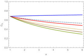
Figure 1: Comparison of the evolution of $\Omega_{\Lambda}-a$ between the LECHDE and the HDE models with the future event horizon cut-off. The dashed, dotted and thick (Green) lines represent the LECHDE model for $c=0.8,1,1.2$, respectively. The Blue, Red and Brown lines indicate the HDE model for $c=0.8,1,1.2$, respectively.

In this figure, we can see that the evolution of $\Omega_{\Lambda}$ with respect to the scale factor for the LECHDE model with $c=0.8,1,1.2$ is faster than the evolution of $\Omega_{\Lambda}$ with respect to the scale factor for the HDE model. In the figure (2), we have plotted the evolution of $\Omega_{\Lambda}$ with respect to $x=\ln(a)$ for the logarithmic entropy-corrected holographic dark energy model for different values of $c=0.8,1,1.2$ gong . We have neglected the change of the inflaton energy density in time for simplicity. We see that as $c$ increases, the energy density $\Omega_{\Lambda}$ becomes more dominated at earlier times.

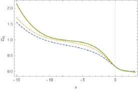
Figure 2: The evolution of $\Omega_{\Lambda}$ with respect to $x=\ln(a)$ for the LECHDE model with the future event horizon cut-off. The dashed, dotted and thick lines represent the LECHDE model for $c=0.8,1,1.2$, respectively. Here, neither $a$ nor $\Omega_{\Lambda}$ are not normalized to $a_{0}=1$ and $0<\Omega_{\Lambda}<1$. The normalization is chosen for numerical convenience. For simplicity, the inflaton energy density is assumed to be constant.

Using Eqs. (10) and (23), we obtain

$$R_{h}=\frac{5c\times 10^{-4}}{M_{P}}\Big{(}\frac{10^{16}GeV}{T_{reh}}\Big{)}^{2}\sqrt{\gamma_{\mu}}.$$ (31)

Note that if $\gamma_{\mu}=1$, then Eq. (31) will reduce to Eq. (14) in Ref chen .

Also, using Eqs. (7), (8), (12), (15), (16), (17), (27) and (28), we obtain

$$\mathcal{R}=\frac{2M_{P}^{2}H^{2}}{\dot{\varphi}^{2}}\Big{(}\frac{\dot{\phi}}{H}+\phi\Big{)}\exp\Big{(}2c^{2}\int_{t}^{t_{LS}}\frac{\gamma_{\mu}}{R_{h}^{2}H}\Big{[}\Big{(}1-\frac{1}{R_{h}H}\Big{)}\Big{(}2-\frac{1}{\gamma_{\mu}}-\frac{\alpha\Omega_{\Lambda}}{9c^{4}\gamma_{\mu}^{2}(1-\Omega_{\Lambda})}\Big{)}\Big{]}dt\Big{)},$$ (32)

where $t_{LS}$ is the time of the Last Scattering Surface. Using (18) and (32), we also obtain

$$\mathcal{P}=\frac{H^{4}}{4\pi^{2}\dot{\varphi}^{2}}\exp\Big{(}4c^{2}\int_{t}^{t_{LS}}\frac{\gamma_{\mu}}{R_{h}^{2}H}\Big{[}\Big{(}1-\frac{1}{R_{h}H}\Big{)}\Big{(}2-\frac{1}{\gamma_{\mu}}-\frac{\alpha\Omega_{\Lambda}}{9c^{4}\gamma_{\mu}^{2}(1-\Omega_{\Lambda})}\Big{)}\Big{]}dt\Big{)}.$$ (33)

Finally, using Eqs. (7), (8), (15), (19), (27) and (28), we find

$$n_{s}-1=-4\epsilon+2\delta-\frac{4c^{2}\gamma_{\mu}}{R_{h}^{2}H^{2}}\Big{[}\Big{(}1-\frac{1}{R_{h}H}\Big{)}\Big{(}2-\frac{1}{\gamma_{\mu}}-\frac{\alpha\Omega_{\Lambda}}{9c^{4}\gamma_{\mu}^{2}(1-\Omega_{\Lambda})}\Big{)}\Big{]}.$$ (34)

If $\alpha=\beta=0$ and $\gamma_{\mu}=1$, then Eqs. (32), (33) and (34) will reduce to Eqs. (20), (21) and (22), respectively in Ref chen .

Now, we derive the corrections to the spectral index produced by the logarithmic entropy-corrected holographic dark energy with the future event horizon cut-off. The slow roll parameter is given by chen

$$\eta\equiv\epsilon+\delta.$$ (35)

Using Eqs. (8), (27) and (28), we have

$$\epsilon=\epsilon_{0}+\frac{c^{2}\gamma_{\mu}}{R_{h}^{2}H^{2}}\Big{[}\Big{(}1-\frac{1}{R_{h}H}\Big{)}\Big{(}2-\frac{1}{\gamma_{\mu}}-\frac{\alpha\Omega_{\Lambda}}{9c^{4}\gamma_{\mu}^{2}(1-\Omega_{\Lambda})}\Big{)}\Big{]},$$ (36)

where $\epsilon_{0}$ is the main contribution in the inflation models without the logarithmic entropy-corrected holographic dark energy. In the above equation, the correction terms are as follows

$$\frac{c^{2}\gamma_{\mu}}{R_{h}^{2}H^{2}}\Big{[}\Big{(}1-\frac{1}{R_{h}H}\Big{)}\Big{(}2-\frac{1}{\gamma_{\mu}}-\frac{\alpha\Omega_{\Lambda}}{9c^{4}\gamma_{\mu}^{2}(1-\Omega_{\Lambda})}\Big{)}\Big{]}.$$

Using Eqs. (34), (35) and (36), we have

$$n_{s}-1=-6\epsilon_{0}+2\eta-\frac{10c^{2}\gamma_{\mu}}{R_{h}^{2}H^{2}}\Big{[}\Big{(}1-\frac{1}{R_{h}H}\Big{)}\Big{(}2-\frac{1}{\gamma_{\mu}}-\frac{\alpha\Omega_{\Lambda}}{9c^{4}\gamma_{\mu}^{2}(1-\Omega_{\Lambda})}\Big{)}\Big{]}.$$ (38)

Here the first and second terms are the standard contributions from the single field inflaton models. Also, because of the last term in Eq. (38), we can see that the effect of the LECHDE model with the future event horizon cut-off is to make the spectrum redder than that of the HDE model. Moreover, using the cosmological data ade (the correction to $n_{s}-1$ should be smaller than -0.05), Eq. (25), and the last term in Eq. (38), we obtain a constraint as follows

$$\frac{2x^{4}}{5y^{2}}\Big{[}\Big{(}1-\frac{x^{2}}{5cy\sqrt{\gamma_{\mu}}}\Big{)}\Big{(}2-\frac{1}{\gamma_{\mu}}-\frac{\alpha x^{4}}{9c^{4}\gamma_{\mu}^{2}(25y^{2}-x^{4})}\Big{)}\Big{]}-0.05<0.$$ (39)

where $x\equiv\frac{T_{reh}}{10^{16}GeV}$, $y\equiv\frac{H}{10^{-4}M_{P}}$ and $\gamma_{\mu}$ is given in terms of $x$, $\alpha,\beta$ and $c$ by solving the following equation

$$\gamma_{\mu}=1+\frac{x^{4}}{75\times 10^{8}c^{4}\gamma_{\mu}}\Big{[}\alpha\ln\Big{(}\frac{25\times 10^{8}c^{2}\gamma_{\mu}}{x^{4}}\Big{)}+\beta\Big{]}.$$ (40)

The inequality (39) constrains the quantities $H,T_{reh},c$, $\alpha$ and $\beta$ at early universe.

IV LECHDE model with particle horizon cut-off in inflation

The particle horizon cut-off is given by

$$R_{H}=a\int_{0}^{t}\frac{dt}{a}.$$ (41)

Taking time derivative of Eq. (41) and using Eq. (41) one can obtain

$$\dot{R_{H}}=HR_{H}+1.$$ (42)

Using Eq. (3) and $L=R_{H}$ we have

$$\rho_{\Lambda}=3c^{2}M_{P}^{2}R_{H}^{-2}+R_{H}^{-4}\Big{[}\alpha\ln(M_{P}^{2}R_{H}^{2})+\beta\Big{]}.$$ (43)

Also, we can write Eq. (43) as follows

$$\rho_{\Lambda}=3c^{2}M_{P}^{2}R_{H}^{-2}\gamma_{\nu},$$ (44)

where

$$\gamma_{\nu}=1+\frac{1}{3c^{2}M_{P}^{2}R_{H}^{2}}\Big{[}\alpha\ln(M_{P}^{2}R_{H}^{2})+\beta\Big{]}.$$ (45)

Using Eq. (44) and inserting in Eq. (4), we have

$$\Omega_{\Lambda}=\frac{c^{2}\gamma_{\nu}}{R_{H}^{2}H^{2}}.$$ (46)

In the flat FRW universe, using Eqs. (5) and (44) for the inflation model and the LECHDE model with the particle horizon cut-off, the Friedmann equation is given by

$$3M_{P}^{2}H^{2}=\frac{1}{2}\dot{\varphi}^{2}+V+3c^{2}M_{P}^{2}R_{H}^{-2}\gamma_{\nu}.$$ (47)

Taking the time derivative of Eq. (47) and using Eqs. (6), (42) and (44) yields

$$-2M_{P}^{2}\dot{H}=\dot{\varphi}^{2}+2c^{2}M_{P}^{2}R_{H}^{-2}\gamma_{\nu}\Big{(}1+\frac{1}{R_{H}H}\Big{)}\Big{[}2-\frac{1}{\gamma_{\nu}}-\frac{\alpha H^{2}\Omega_{\Lambda}}{3c^{2}M_{P}^{2}\gamma_{\nu}^{2}}\Big{]}.$$ (48)

Using Eqs. (46), (47) and the slow-roll conditions, we obtain the Friedmann equation as follows

$$\frac{1}{H}=\sqrt{1-\Omega_{\Lambda}}\sqrt{\frac{3M_{P}^{2}}{V}}.$$ (49)

Taking time derivative of Eq. (4) and using Eqs. (4), (42), (44), (45), (48), (49) and the slow-roll conditions, we have

$$\Omega_{\Lambda}^{{}^{\prime}}=-2\Omega_{\Lambda}\Big{(}1-\Omega_{\Lambda}\Big{)}\Big{(}1+\frac{\sqrt{\Omega_{\Lambda}}}{c\sqrt{\gamma_{\nu}}}\Big{)}\Big{[}2-\frac{1}{\gamma_{\nu}}-\frac{\alpha\Omega_{\Lambda}V}{9c^{4}M_{P}^{4}\gamma_{\nu}^{2}(1-\Omega_{\Lambda})}\Big{]}.$$ (50)

Now, we assume $V=M_{P}^{4}$ david and insert in Eq. (50) to obtain

$$\Omega_{\Lambda}^{{}^{\prime}}=-2\Omega_{\Lambda}\Big{(}1-\Omega_{\Lambda}\Big{)}\Big{(}1+\frac{\sqrt{\Omega_{\Lambda}}}{c\sqrt{\gamma_{\nu}}}\Big{)}\Big{[}2-\frac{1}{\gamma_{\nu}}-\frac{\alpha\Omega_{\Lambda}}{9c^{4}\gamma_{\nu}^{2}(1-\Omega_{\Lambda})}\Big{]}.$$ (51)

Similar to the previous case, in the figure (3), we have plotted numerically the evolution of $\Omega_{\Lambda}$ with respect to the scale factor for the logarithmic entropy-corrected holographic dark energy model with the particle horizon cut-off and the ordinary holographic dark energy model HDE with $c=0.8,1,1.2$ chen , gong . Note that if $\alpha=\beta=0$ and $\gamma_{\nu}=1$, then Eq. (50) will reduce to Eq. (34) in Ref chen and this means that the LECHDE model will reduce to the HDE model. In this figure, we can see that unlike the previous case the evolution of $\Omega_{\Lambda}$ with respect to the scale factor for the LECHDE model with $c=0.8,1,1.2$ is slower than the evolution of $\Omega_{\Lambda}$ with respect to the scale factor for the HDE model.

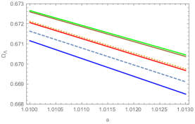
Figure 3: The comparison evolution $\Omega_{\Lambda}-a$ between the LECHDE and the HDE models with the particle horizon cut-off for two models. The dashed, dotted and thick (Green) lines represent the LECHDE model for $c=0.8,1,1.2$, respectively. The Blue, Red and Brown lines indicate the HDE model for $c=0.8,1,1.2$, respectively.

In the figure (4), we have plotted the evolution of $\Omega_{\Lambda}$ with respect to $x=\ln(a)$ for the logarithmic entropy-corrected holographic dark energy model with $c=0.8,1,1.2$ gong . For simplicity, we have neglected the change of the inflaton energy density with time. We see that as $c$ increases, the energy density $\Omega_{\Lambda}$ becomes more dominated at earlier times.

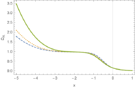
Figure 4: The evolution $\Omega_{\Lambda}$ respect to $x=\ln(a)$ for the LECHDE model with the particle horizon cut-off. The dashed, dotted and thick lines represent the LECHDE model for $c=0.8,1,1.2$, respectively. Here, neither $a$ nor $\Omega_{\Lambda}$ are not normalized to $a_{0}=1$ and $0<\Omega_{\Lambda}<1$. The normalization is chosen for numerical convenience. For simplicity, the inflaton energy density is assumed to be constant.

Using Eqs. (10) and (44), we obtain

$$R_{H}=\frac{5c\times 10^{-4}}{M_{P}}\Big{(}\frac{10^{16}GeV}{T_{reh}}\Big{)}^{2}\sqrt{\gamma_{\nu}}.$$ (52)

Also, using Eqs. (7), (8), (12), (15), (16), (17), (48) and (49), we find

$$\mathcal{R}=\frac{2M_{P}^{2}H^{2}}{\dot{\varphi}^{2}}\Big{(}\frac{\dot{\phi}}{H}+\phi\Big{)}\exp\Big{(}2c^{2}\int_{t}^{t_{LS}}\frac{\gamma_{\nu}}{R_{H}^{2}H}\Big{[}\Big{(}1+\frac{1}{R_{H}H}\Big{)}\Big{(}2-\frac{1}{\gamma_{\nu}}-\frac{\alpha\Omega_{\Lambda}}{9c^{4}\gamma_{\nu}^{2}(1-\Omega_{\Lambda})}\Big{)}\Big{]}dt\Big{)}.$$ (53)

Using (18) and (53) yields

$$\mathcal{P}=\frac{H^{4}}{4\pi^{2}\dot{\varphi}^{2}}\exp\Big{(}4c^{2}\int_{t}^{t_{LS}}\frac{\gamma_{\nu}}{R_{H}^{2}H}\Big{[}\Big{(}1+\frac{1}{R_{H}H}\Big{)}\Big{(}2-\frac{1}{\gamma_{\nu}}-\frac{\alpha\Omega_{\Lambda}}{9c^{4}\gamma_{\nu}^{2}(1-\Omega_{\Lambda})}\Big{)}\Big{]}dt\Big{)}.$$ (54)

Using Eqs. (7), (8), (15), (19), (48) and (49), we have

$$n_{s}-1=-4\epsilon+2\delta-\frac{4c^{2}\gamma_{\nu}}{R_{H}^{2}H^{2}}\Big{[}\Big{(}1+\frac{1}{R_{H}H}\Big{)}\Big{(}2-\frac{1}{\gamma_{\nu}}-\frac{\alpha\Omega_{\Lambda}}{9c^{4}\gamma_{\nu}^{2}(1-\Omega_{\Lambda})}\Big{)}\Big{]}.$$ (55)

For $\alpha=\beta=0$ and $\gamma_{\nu}=1$, Eqs. (53), (54) and (55) will reduce to Eqs. (35), (36) and (37), respectively in Ref chen . Using Eqs. (8), (48) and (49), we obtain

$$\epsilon=\epsilon_{0}+\frac{c^{2}\gamma_{\nu}}{R_{H}^{2}H^{2}}\Big{[}\Big{(}1+\frac{1}{R_{H}H}\Big{)}\Big{(}2-\frac{1}{\gamma_{\nu}}-\frac{\alpha\Omega_{\Lambda}}{9c^{4}\gamma_{\nu}^{2}(1-\Omega_{\Lambda})}\Big{)}\Big{]},$$ (56)

where $\epsilon_{0}$ is the main contribution in the inflation models without the logarithmic entropy-corrected holographic dark energy. In the above equation, the correction terms are as follows

$$\frac{c^{2}\gamma_{\nu}}{R_{H}^{2}H^{2}}\Big{[}\Big{(}1+\frac{1}{R_{H}H}\Big{)}\Big{(}2-\frac{1}{\gamma_{\nu}}-\frac{\alpha\Omega_{\Lambda}}{9c^{4}\gamma_{\nu}^{2}(1-\Omega_{\Lambda})}\Big{)}\Big{]}.$$

Using Eqs. (35), (55) and (56), we find

$$n_{s}-1=-6\epsilon_{0}+2\eta-\frac{10c^{2}\gamma_{\nu}}{R_{H}^{2}H^{2}}\Big{[}\Big{(}1+\frac{1}{R_{H}H}\Big{)}\Big{(}2-\frac{1}{\gamma_{\nu}}-\frac{\alpha\Omega_{\Lambda}}{9c^{4}\gamma_{\nu}^{2}(1-\Omega_{\Lambda})}\Big{)}\Big{]}.$$ (58)

As in the previous case, we can see that the effect of the LECHDE model with the particle horizon cut-off is to make the spectrum redder. Using the cosmological data ade (the correction to $n_{s}-1$ should be smaller than -0.05), Eq. (46), and the last term in Eq. (58), we obtain a constraint as follows

$$\frac{2x^{4}}{5y^{2}}\Big{[}\Big{(}1+\frac{x^{2}}{5cy\sqrt{\gamma_{\nu}}}\Big{)}\Big{(}2-\frac{1}{\gamma_{\nu}}-\frac{\alpha x^{4}}{9c^{4}\gamma_{\nu}^{2}(25y^{2}-x^{4})}\Big{)}\Big{]}-0.05<0.$$ (59)

where $x\equiv\frac{T_{reh}}{10^{16}GeV}$, $y\equiv\frac{H}{10^{-4}M_{P}}$ and $\gamma_{\nu}$ is given in terms of $x$, $\alpha,\beta$ and $c$ by solving the following equation

$$\gamma_{\nu}=1+\frac{x^{4}}{75\times 10^{8}c^{4}\gamma_{\nu}}\Big{[}\alpha\ln\Big{(}\frac{25\times 10^{8}c^{2}\gamma_{\nu}}{x^{4}}\Big{)}+\beta\Big{]}.$$ (60)

The inequality (59) constrains the quantities $H,T_{reh},c$, $\alpha$ and $\beta$ at early universe.

V LECHDE model with Hubble cut-off in inflation

The hubble cut-off is given by

$$L=H^{-1}.$$ (61)

Using Eqs. (3) and (61) we find

$$\rho_{\Lambda}=3c^{2}M_{P}^{2}H^{2}+H^{4}\Big{[}\alpha\ln(M_{P}^{2}H^{-2})+\beta\Big{]}.$$ (62)

Also, we can write Eq. (62) as follows

$$\rho_{\Lambda}=3c^{2}M_{P}^{2}H^{2}\gamma_{\theta},$$ (63)

Where

$$\gamma_{\theta}=1+\frac{H^{2}}{3c^{2}M_{P}^{2}}\Big{[}\alpha\ln(M_{P}^{2}H^{-2})+\beta\Big{]}.$$ (64)

Using Eq. (63) and inserting in Eq. (4), we have

$$\Omega_{\Lambda}=c^{2}\gamma_{\theta}.$$ (65)

In the flat FRW universe, using Eqs. (5) and (63) for the inflation model and the LECHDE model with the Hubble cut-off, the Friedmann equation is given by

$$3M_{P}^{2}H^{2}=\frac{1}{2}\dot{\varphi}^{2}+V+3c^{2}M_{P}^{2}H^{2}\gamma_{\theta}.$$ (66)

Now, taking time derivative of Eq. (64) and using Eq. (64) yields

$$\dot{\gamma_{\theta}}=\dot{H}\Big{[}\frac{2(\gamma_{\theta}-1)}{H}-\frac{2\alpha H}{3c^{2}M_{P}^{2}}\Big{]}.$$ (67)

Also, taking time derivative of Eq. (66) and using Eqs. (6), (63) and (67) leads to

$$-2M_{P}^{2}\dot{H}\Big{[}1-c^{2}\Big{(}2\gamma_{\theta}-1\Big{)}+\frac{\alpha H^{2}}{3M_{P}^{2}}\Big{]}=\dot{\varphi}^{2}.$$ (68)

Using Eqs. (65), (66) and the slow-roll conditions, the Friedmann equation is obtained as follows

$$\frac{1}{H}=\sqrt{1-\Omega_{\Lambda}}\sqrt{\frac{3M_{P}^{2}}{V}}.$$ (69)

Using Eqs. (7), (8), (12), (15), (16), (17), (68) and (69), we obtain

$$\mathcal{R}=\frac{2M_{P}^{2}H^{2}}{\dot{\varphi}^{2}}\Big{(}\frac{\dot{\phi}}{H}+\phi\Big{)}\exp\Big{[}2\int_{t}^{t_{LS}}\frac{dH}{H}\Big{(}c^{2}(2\gamma_{\theta}-1)-\frac{\alpha}{9(1-\Omega_{\Lambda})}\Big{)}\Big{]}.$$ (70)

Using (18) and (70), we find

$$\mathcal{P}=\frac{H^{4}}{4\pi^{2}\dot{\varphi}^{2}}\exp\Big{[}4\int_{t}^{t_{LS}}\frac{dH}{H}\Big{(}c^{2}(2\gamma_{\theta}-1)-\frac{\alpha}{9(1-\Omega_{\Lambda})}\Big{)}\Big{]}.$$ (71)

And, using Eqs. (7), (8), (15), (19), (68) and (69), we have

$$n_{s}-1=2\delta-\epsilon\Big{[}4+4c^{2}\Big{(}2\gamma_{\theta}-1\Big{)}-\frac{\alpha}{9(1-\Omega_{\Lambda})}\Big{]}.$$ (72)

We assume $V=M_{P}^{4}$ david and insert Eq. (69) in Eq. (64) to obtain

$$\gamma_{\theta}=1+\frac{1}{9c^{2}\Big{(}1-\Omega_{\Lambda}\Big{)}}\Big{[}\ln\Big{(}3-3\Omega_{\Lambda}\Big{)}+1\Big{]}.$$ (73)

In the $\Omega_{\Lambda}\longrightarrow 0$ limit, Eq. (73) yields

$$\gamma_{\theta}=1+\frac{0.233}{c^{2}}.$$ (74)

Now in the $\Omega_{\Lambda}\longrightarrow 0$ limit and using Eq. (74), Eqs. (70), (71) and (72) will change as follows

$$\mathcal{R}=\frac{2M_{P}^{2}H^{2+2c^{2}+0.71}}{M^{-2c^{2}-0.71}\dot{\varphi}^{2}}\Big{(}\frac{\dot{\phi}}{H}+\phi\Big{)},$$ (75)

$$\mathcal{P}=\frac{H^{4+4c^{2}+1.42}}{4\pi^{2}M^{4c^{2}+1.42}\dot{\varphi}^{2}},$$ (76)

$$n_{s}-1=-\epsilon\Big{(}4+4c^{2}+1.753\Big{)}+2\delta,$$ (77)

where $M$ is a constant with the dimension of energy. We compare Eqs. (75), (76) and (77) with Eqs. (42), (43) and (44) in Ref chen . Then, we can write the above equations as follows

$$\mathcal{R}_{LECHDE}=\mathcal{R}_{HDE}\frac{H^{0.71}}{M^{-0.71}},$$ (78)

$$\mathcal{P}_{LECHDE}=\mathcal{P}_{HDE}\frac{H^{1.42}}{M^{1.42}},$$ (79)

$$(n_{s}-1)_{LECHDE}={(n_{s}-1)}_{HDE}-1.753\epsilon~{}.$$ (80)

It is seen that in the $\Omega_{\Lambda}\longrightarrow 0$ limit the effect of the LECHDE model with the Hubble cut-off is to make the spectrum redder than that of the HDE model.

VI Concluding remarks

In this work, we have investigated the inflation by logarithmic entropy-corrected holographic dark energy LECHDE model for different cut-offs. We have assumed that the inflaton field does not couple to the logarithmic entropy-corrected holographic dark energy and hence it is not affected by the existence of the logarithmic entropy-corrected holographic dark energy. Also, we have assumed that the LECHDE model depends on the background and it does not create the perturbations. Therefore, the standard perturbation equations remain unchanged. We have also assumed that the reheating period occurs immediately after the inflation period. Considering these assumptions, we have compared our results for the LECHDE model with the results of the HDE model obtained in chen . We have found that for the future event horizon cut-off (see figure (1)), the evolution of $\Omega_{\Lambda}$ with respect to the scale factor for the LECHDE model is faster than that of the HDE model. Also, in the evolution of $\Omega_{\Lambda}$ with respect to $x=\ln(a)$, we obtained that as $c$ increases, the energy density $\Omega_{\Lambda}$ becomes more dominated at earlier times for the LECHDE model compared with the HDE model. For the particle horizon cut-off (see figure (3)), we have found that the evolution of $\Omega_{\Lambda}$ with respect to the scale factor for the LECHDE model is slower than that of the HDE model. Also, in the evolution of $\Omega_{\Lambda}$ with respect to $x=\ln(a)$, we obtained that as $c$ increases, the energy density $\Omega_{\Lambda}$ becomes more dominated at earlier times for the LECHDE model compared with the HDE model.

We have derived the corrections to the spectral index produced by the LECHDE model with the event future horizon, the particle horizon and the hubble horizon cut-offs, and found that the effect of the LECHDE model for all three cut offs is making the spectrum redder than the HDE model. The requirement of consistency with the observational data in LECHDE model of inflation, constrains the reheating temperature and Hubble parameter by one parameter of holographic dark energy and two new parameters of logarithmic corrections, compared to the HDE model.

References

(1) A. G. Riess, et al., Astron. J. 116 (1998) 1009;
S. Perlmutter, et al., Astrophys. J. 517 (1999) 565;
P. de Bernardis, et al., Nature 404 (2000) 955;
S. perlmutter, et al., Astrophys. J. 598 (2003) 102.
(2) E. J. Copeland, M. Sami, S. Tsujikawa, IJMPD, 15 (2066)
1753.
(3) S. Weinberg, Reviews of modern physics, 61 (1989) 1.
(4) T. Padmanabhan, Phys. Rept. 380 (2006) 235.
(5)A. G. Cohen, D. B. Kaplan, and A. E. Nelson, Phys. Rev. Lett. 82, (1999) 4971; S. D. H. Hsu, Phys. Lett. B 594, (2004) 13.
(6)M. Li, Phys. Lett. B 603, (2004) 1.
(7) H. Wei, R. G. Cai, Phys. Lett. B 660 (2008) 113.
(8) Y. F. Cai, E. N. Saridakis, M. R. Setare, J. Q. Xia, Phys.
Rept. 493 (2010) 1.
(9) M. R. Setare, Phys. Lett. B 653 (2007) 116.
(10) M. R. Setare, J. sadeghi, A. R. Amani, Phys. Lett. B 673
(2009) 241.
(11) L. Susskind, J. Math. Phys. 36 (1995) 6377;
S. Nojiri, S. D. Odintsov, Gen. Rel. Grav. 38 (1285) 1285;
K. Bamba, S. Capozziello, S. D. Odintsov, Astrophys. Space Sci. 342 (2012)
155.
(12) R. M. Wald, Phys. Rev. D 48 (1993) 3427.
(13) R. Banerjee, B. R. Majhi, Phys. Lett. B 662 (2008) 62;
R. Banerjee, B. R. Majhi, JHEP 06 (2008) 095;
J. Zhang, Phys. Lett. B 668 (2008) 353.
(14) Y. F. Cai, J. Liu, H. Li, Phys. Lett. B 690 (2010) 213.
(15) H. Wei, Commun. Theor. Physics, 52 (2009) 743.
(16) B. Chen, M. Li, Y. Wang, Nucl. Phys. B 774 (2007) 256.
(17) D. H. Lyth, A. Riotto, Phys. Rept. 314 (1999) 1.
(18) Q. G. Huang, Y. Gong, JCAP 0408 (2004) 006;
H. C. Kao, W. L. Lee, F. L. Lin, Phys. Rev. D 71 (2005) 123518;
X. Zhang, Int. J. Mod. Phys. D 14 (2005) 1597;
X. Zhang, F. Q. Wu, Phys. Rev. D 72 (2005) 043524;
Z. Chang, F. Q. Wu, X. Zhang, Phys. Lett. B 633 (2006) 14;
X. Zhang, Int. J. Mod. Phys. D 74 (2006) 103505.
(19) V. F. Mukhanov, H. A. Feldman, R. H. Brandenberger, Phys.
Rept. 215 (1992) 203.
(20) B. Chen, M. Li, T. Wang, Y. Wang, Mod. Phys. Lett. A 22 (2007)
1987.
(21) P. A. R. Ade, et al., Astron. Astrophys. 571 (2014) A 22.