The universal C*-algebra of the electromagnetic field  II. Topological charges and spacelike linear fields
Dedicated to Karl-Henning Rehren on the occasion of his 60th birthday

Abstract. Conditions for the appearance of topological charges are studied in the framework of the universal C*-algebra of the electromagnetic field, which is represented in any theory describing electromagnetism. It is shown that non-trivial topological charges, described by pairs of fields localised in certain topologically non-trivial spacelike separated regions, can appear in regular representations of the algebra only if the fields depend non-linearly on the mollifying test functions. On the other hand, examples of regular vacuum representations with non-trivial topological charges are constructed, where the underlying field still satisfies a weakened form of “spacelike linearity”. Such representations also appear in the presence of electric currents. The status of topological charges in theories with several types of electromagnetic fields, which appear in the short distance (scaling) limit of asymptotically free non-abelian gauge theories, is also briefly discussed.
Mathematics Subject Classification.  81V10, 81T05, 14F40
Keywords.  electromagnetic field, topological charges, non-linear field operators

1 Introduction

A universal C*-algebra for the description of the electromagnetic field has recently been constructed in [7]. It was argued there that representations of this algebra appear in any theory describing electromagnetism. The algebra does not contain any specific dynamical information, yet such information can be obtained from it by (i) choosing in its dual space some suitable pure state, (ii) proceeding to its GNS representation and (iii) considering the quotient of the algebra with regard to the kernel of this representation. In this way one obtains all theories of the electromagnetic field which comply with the Haag-Kastler axioms [13].

It was observed in this analysis that there exist representations of the universal algebra with non-trivial topological charges. These charges are given by the commutator of operators, describing the intrinsic (gauge invariant) vector potential, which have their supports in certain spacelike separated, topologically non-trivial regions (precise definitions are given below). As was shown in [7], such commutators need not vanish, but they are elements of the centre of the algebra. The arguments given in [7] for the existence of states where these commutators have values different from zero, indicating non-trivial topological charges, led only to an abstract existence theorem, however. In particular, the conditions for the existence of these charges remained unclear. It is the aim of the present investigation to clarify this point.

We will show that in all regular pure states on the algebra, where one can define the vector potential, the topological charges vanish whenever this potential depends linearly on the underlying test functions. In particular, such charges cannot appear in the Wightman framework. Yet the condition of unrestrained linearity of quantum fields on test functions does not have a clear-cut operational basis and seems more a matter of convenience. In particular, the Haag-Kastler framework of quantum field theory does not rely on such a condition and non-linear quantum fields already appeared in other contexts, cf. for example [8, Eq. 4] and [5, Rem. 6.1].

Within the present framework of the universal algebra, we will exhibit regular vacuum states with non-trivial topological charges. There the resulting vector potentials are homogeneous on the space of test functions, but they have the property of additivity only for test functions with spacelike separated supports (i.e. the potentials are spacelike linear). Our first example is based on a reinterpretation of the theory of the free electromagnetic field. We then show that such states also exist in the presence of non-trivial electric currents.

We also consider theories of several electromagnetic fields which are described by suitable extensions of the universal algebra. One may expect that these theories cover the scaling (short distance) limit of non-abelian gauge fields in view of their expected property of asymptotic freedom. It is of interest that in these theories there exist regular vacuum states with non-trivial topological charges where the corresponding vector potentials depend linearly on test functions. The topological charges are given there by the commutator of spacelike separated operators describing different potentials. It is an intriguing question whether such charges might manifest themselves already at finite scales in gauge theory.

In the subsequent section we recall from [7] some basic properties of the universal algebra. Sec. 3 contains the proof that regular pure states carrying a non-trivial topological charge give rise to non-linear vector potentials. In Sec. 4 we exhibit a vacuum state with vanishing electric current which carries a topological charge. That such vacuum states also exist for non-trivial electric currents is shown in Sec. 5. Examples of states carrying a topological charge in theories with several fields are presented in Sec. 6. The article closes with some brief conclusions.

2 Preliminaries

Conventionally, the electromagnetic field $F$ is described by an operator valued map $f\mapsto F(f)$, where $f\in{\mathscr{D}}_{2}({\mathbb{R}}^{4})$ are compactly supported real test functions with values in the antisymmetric tensors of rank two [17, 18]. As is well known, the homogeneous Maxwell equations imply that this field can conveniently be described by an intrinsic (gauge invariant) vector potential $g\mapsto A(g)$, where $g\in{\mathscr{C}}_{1}({\mathbb{R}}^{4})$, the space of real vector valued test functions that are co-closed, i.e. satisfy $\delta g=0$. Here $\delta$ denotes the co-derivative (generalised divergence) which is related to the exterior derivative $d$ (generalised curl) by $\delta=-\star d\star$ and $\star$ is the Hodge operator. Recalling that $\delta^{2}=0$, the electromagnetic field and the potential are related by $F(f)\doteq A(\delta f)$, $f\in{\mathscr{D}}_{2}({\mathbb{R}}^{4})$, and the electric current is defined by $j(h)\doteq A(\delta dh)$ for real vector valued test functions $h\in{\mathscr{D}}_{1}({\mathbb{R}}^{4})$.

In [7] the properties of the intrinsic vector potential were cast into a C*-algebraic setting by formally proceeding from $A(g)$ to unitary operators $V(a,g)\,\hat{=}\,e^{\,iaA(g)}$. More precisely, one proceeds from the free *-algebra, generated by the symbols $V(a,g)$, where $a\in{\mathbb{R}}$, $g\in{\mathscr{C}}_{1}({\mathbb{R}}^{4})$, and takes its quotient with regard to the ideal generated by the relations

$$V(a_{1},g)V(a_{2},g)=V(a_{1}+a_{2},g)\,,\ \ V(a,g)^{*}=V(-a,g)\,,\ \ V(0,g)=1$$ (2.1)

$$V(a_{1},g_{1})V(a_{2},g_{2})=V(1,a_{1}g_{1}+a_{2}g_{2})\,\ \ \mbox{if}\ \ \mbox{supp}\,g_{1}\,\mbox{\Large$\times$}\,\mbox{supp}\,g_{2}$$ (2.2)

$$\lfloor V(a,g)\,,\lfloor V(a_{1},g_{1}),V(a_{2},g_{2})\rfloor\rfloor=1\,\ \ \mbox{for any $g$ if}\ \ \mbox{supp}\,g_{1}\perp\mbox{supp}\,g_{2}\,.$$ (2.3)

Relation (2.1) subsumes the algebraic properties of unitary one-parameter groups $a\mapsto V(a,g)$, expressing the idea that one is dealing with the exponential functions of the potential, mollified with test functions $g\in{\mathscr{C}}_{1}({\mathbb{R}}^{4})$. Relation (2.2) encodes restricted linearity and locality properties of the vector potential, where the symbol  $\times$ marks pairs of regions that can be separated by two opposite characteristic wedges (e.g. spacelike separated double cones). The symbol $\lfloor\cdot,\cdot\rfloor$ in relation (2.3) indicates the group theoretic commutator of unitary operators; this relation embodies the information that the commutator of operators which are localised in arbitrary spacelike separated regions, marked by the symbol $\perp$, is a central element. These operators therefore determine in general superselected quantities which, in view of their topological nature, are called topological charges. Note that these conditions are slightly weaker than the corresponding ones in [7]. They simplify the discussion of the topological charges which are of interest here.

As has been shown in [7], the *-algebra ${\mathfrak{V}}_{0}$ generated by the unitaries $V(a,g)$ with $g\in{\mathscr{C}}_{1}({\mathbb{R}}^{4})$, $a\in{\mathbb{R}}$, can be equipped with a C*-norm generated by all of its GNS representations. Proceeding to the completion of ${\mathfrak{V}}_{0}$ with regard to this norm, one obtains the universal C*-algebra ${\mathfrak{V}}$ of the electromagnetic field.

As already mentioned, the algebra ${\mathfrak{V}}$ does not contain any dynamical information. But since the Poincaré transformations $P\in\pazocal{P}_{+}^{\uparrow}$ act on ${\mathfrak{V}}$ by automorphisms $\alpha_{P}$ which are defined on the generating unitaries by $\alpha_{P}(V(a,g))=V(a,g_{P})$, where $g_{P}$ is the Poincaré transformed test function $g$, one can identify the vacuum states in the dual space of ${\mathfrak{V}}$. Picking any such (pure) vacuum state $\omega$ and proceeding to its GNS representation $(\pi,\pazocal{H},\Omega)$, one obtains a faithful representation of the quotient algebra ${\mathfrak{V}}/\mbox{ker}\pi$, where the Poincaré transformations are unitarily implemented. In this way one can in principle describe any dynamics of the electromagnetic field in a manner which is compatible with the Haag-Kastler axioms [7].

If one wants to recover in a representation from the unitaries $V(a,g)$ the underlying vector potential, one has to restrict attention to states $\omega$ that are (strongly) regular. This means that the functions $a_{1},\dots,a_{n}\mapsto\omega(V(a_{1},g_{1})\cdots V(a_{n},g_{n}))$ are smooth for arbitrary test functions $g_{1},\dots,g_{n}\in{\mathscr{C}}_{1}({\mathbb{R}}^{4})$ and $n\in{\mathbb{N}}$. One then finds [7] that in the corresponding GNS representation $(\pi,\pazocal{H},\Omega)$ one has $\pi(V(a,g))=e^{iaA_{\pi}(g)}$ for $a\in{\mathbb{R}}$, $g\in{\mathscr{C}}_{1}({\mathbb{R}}^{4})$. Here $A_{\pi}(g)$ are selfadjoint operators with a common core $\pazocal{D}\subset\pazocal{H}$ that is stable under their action and includes the vector $\Omega$. Moreover, as a consequence of relation (2.2), these operators are spacelike linear in the sense that they satisfy on $\pazocal{D}$ the equality $a_{1}\,A_{\pi}(g_{1})+a_{2}\,A_{\pi}(g_{2})=A_{\pi}(a_{1}g_{1}+a_{2}g_{2})$ whenever $\mbox{supp}\,g_{1}\mbox{\Large$\times$}\mbox{supp}\,g_{2}$.

If the potential resulting from some regular pure state is also linear in the usual sense, then this state carries no topological charges, as is shown in the subsequent section. More precisely, one then has $[A_{\pi}(g_{1}),A_{\pi}(g_{2})]=0$ whenever $g_{1},g_{2}$ have spacelike separated supports in linked, loop-shaped regions. Yet, as we shall see, there exist also regular vacuum states where these commutators have non-trivial values and the underlying fields are still spacelike linear.

3 Symplectic forms and absence of topological charges

In order to clarify the conditions for the existence of non-trivial topological charges, we consider in this section regular pure states $\omega$ on the universal algebra ${\mathfrak{V}}$ with corresponding GNS representation $(\pi,\pazocal{H},\Omega)$; note that we do not require here that these states describe the vacuum. In complete analogy to the preceding discussion, the regularity of a state $\omega$ implies that for any $g\in{\mathscr{C}}_{1}({\mathbb{R}}^{4})$ there exists a selfadjoint operator $A_{\pi}(g)$ in the corresponding representation. These operators are the generators of the unitary groups $a\mapsto\pi(V(a,g))$ and have a common stable core $\pazocal{D}$ that includes the vector $\Omega$. It then follows from relation (2.3) that whenever $\mbox{supp}\,g_{1}\perp\mbox{supp}\,g_{2}$, the commutator $[A_{\pi}(g_{1}),A_{\pi}(g_{2})]$ is affiliated with the centre of the weak closure $\pi({\mathfrak{V}})^{-}$ of the represented algebra. Since the underlying state was assumed to be pure, the elements of the centre, hence also these commutators, are multiples of the identity. So their expectation values do not depend on the chosen state within the representation and this brings us to define the real form

$$\sigma_{\pi}(g_{1},g_{2})\doteq i\,\langle\Omega,[A_{\pi}(g_{1}),A_{\pi}(g_{2})]\,\Omega\rangle\quad\text{for any}\quad g_{1},g_{2}\in{\mathscr{C}}_{1}({\mathbb{R}}^{4})\,.$$ (3.1)

Now according to relation (2.2), the operators $A_{\pi}$ are in general only spacelike linear. But, depending on the choice of state, they may also be (real) linear on ${\mathscr{C}}_{1}({\mathbb{R}}^{4})$. In the latter case the form $\sigma_{\pi}$ given above defines a bilinear, skew symmetric (symplectic) form on ${\mathscr{C}}_{1}({\mathbb{R}}^{4})$.

We shall show that such symplectic forms $\sigma_{\pi}$ vanish for any pair of test functions $g_{1},g_{2}\in{\mathscr{C}}_{1}({\mathbb{R}}^{4})$ having their supports in certain spacelike separated, linked loop-shaped regions. Whence the corresponding topological charges vanish. An open, bounded region $\pazocal{L}\subset{\mathbb{R}}^{4}$ is said to be loop-shaped if there exists in its interior some spacelike (hence simple) loop $[0,1]\ni t\mapsto\gamma(t)$, consisting of points which are spacelike separated from each other, to which it can continuously be retracted. Thus, $\gamma$ is a deformation retract of $\pazocal{L}$ and therefore homotopy equivalent (homotopic) to $\pazocal{L}$. Simple examples of linked loop-shaped regions are depicted in figure 1.

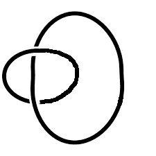
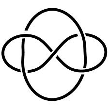
Figure 1: Linked loop-shaped regions: Hopf link and Whitehead link

For the proof of these statements, let $\pazocal{L}\subset{\mathbb{R}}^{4}$ be loop-shaped with corresponding loop $\gamma$ and let $\pazocal{O}_{0}\subset{\mathbb{R}}^{4}$ be a sufficiently small neighbourhood of the origin such that $(\pazocal{O}_{0}+\gamma)\subset\pazocal{L}$. Then, for any real scalar test function $s\in{\mathscr{D}}_{0}({\mathbb{R}}^{4})$ with support in $\pazocal{O}_{0}$, we define a corresponding loop function $x\mapsto l_{s,\gamma}(x)\doteq\int_{0}^{1}dt\ s(x-\gamma(t))\,\overset{\scalebox{0.4}{\textbullet}}{\gamma}(t)$, where $\overset{\scalebox{0.4}{\textbullet}}{\gamma}$ denotes the derivative of $\gamma$. One easily checks that $l_{s,\gamma}\in{\mathscr{C}}_{1}({\mathbb{R}}^{4})$ and that it has support in $(\pazocal{O}_{0}+\gamma)\subset\pazocal{L}$. Moreover, if $\int\!dx\,s(x)\neq 0$ there is no $f\in{\mathscr{D}}_{2}({\mathbb{R}}^{4})$ with support in $\pazocal{L}$ such that $l_{s,\gamma}=\delta f$, i.e.  $l_{s,\gamma}$ is co-closed but not co-exact in this region. As has been pointed out in [7], this fact is crucial for the appearance of non-trivial topological charges. We will restrict attention here to charges of this particular type.

The following lemma shows that for given loop-shaped region $\pazocal{L}$ and any function $g\in{\mathscr{C}}_{1}({\mathbb{R}}^{4})$, having support in $\pazocal{L}$, one finds within its co-cohomology class (referring to the co-derivative) loop functions $l_{s,\gamma}$, as given above.

Lemma 3.1.

Let $g\in{\mathscr{C}}_{1}({\mathbb{R}}^{4})$ have support in a loop-shaped region $\pazocal{L}$. There exist some loop function $l_{s,\gamma}\in{\mathscr{C}}_{1}({\mathbb{R}}^{4})$ and some $f\in{\mathscr{D}}_{2}({\mathbb{R}}^{4})$, both having their support in $\pazocal{L}$, such that $g=l_{s,\gamma}+\delta f$. Hence $g$ and $l_{s,\gamma}$ lie in the same co-cohomology class relative to $\pazocal{L}$.

Proof.

This statement is equivalent to the statement that $\star g=\star l_{s,\gamma}+d\star f$, where $\star$ is the Hodge operator. In other words, the cohomology classes of these functions must be related by $[\star g]=[\star l_{s,\gamma}]\in H_{c}^{3}(\pazocal{L})$, where $H_{c}^{3}(\pazocal{L})$ denotes the third compact de Rham cohomology group of forms which are compactly supported in the given open region. Making use of Poincaré duality [12, Thm. 5.12] and then of the fact that $\pazocal{L}$ is homotopic to $\gamma$ which, being simple, is homotopic to $S^{1}$, we get

$$H_{c}^{3}(\pazocal{L})^{*}\approx H^{1}(\pazocal{L})\approx H^{1}(\gamma)\approx H^{1}(S^{1})\approx{\mathbb{R}}\,.$$ (3.2)

Here $H_{c}^{3}(\pazocal{L})^{*}$ stands for the algebraic dual of $H_{c}^{3}(\pazocal{L})$,  $H^{1}(\,\cdot\,)$ denotes the first cohomology group of the respective regions, and the symbol  $\approx$ indicates isomorphisms between the cohomology groups. Since $H_{c}^{3}(\pazocal{L})^{*}$ is finite dimensional, one has $H_{c}^{3}(\pazocal{L})^{*}\approx H_{c}^{3}(\pazocal{L})$ which implies $H_{c}^{3}(\pazocal{L})\approx{\mathbb{R}}$.

Now let $l_{s,\gamma}$ be any of the loop functions constructed above. Then $\star l_{s,\gamma}$ has support in $\pazocal{L}$ and $d\star l_{s,\gamma}=-\star\delta l_{s,\gamma}=0$ since $l_{s,\gamma}$ is co-closed. Moreover, $\star l_{s,\gamma}$ is exact iff $l_{s,\gamma}$ is co-exact which is the case iff $\int\!dx\,s(x)=0$ for the underlying scalar function $s$, cf. [15, §1] and the subsequent section for a proof. Since the possible values of $\int\!dx\,s(x)$  exhaust ${\mathbb{R}}$ and $H_{c}^{3}(\pazocal{L})\approx{\mathbb{R}}$, it follows that within the cohomology class of any given $\star g$ one can find the Hodge dual of a loop function, $\star l_{s,\gamma}$, proving the statement. ∎

The following statement concerning the forms $\sigma_{\pi}$ in (3.1) is a consequence of the preceding result and the causal Poincaré lemma, established in the appendix of [7].

Lemma 3.2.

Let $\pazocal{L}_{1}$, $\pazocal{L}_{2}$ be two spacelike separated loop-shaped regions and let $g_{1},g_{2}\in{\mathscr{C}}_{1}({\mathbb{R}}^{4})$ have support in $\pazocal{L}_{1}$, respectively $\pazocal{L}_{2}$. Moreover, let $\sigma_{\pi}$ be linear in both entries. There are loop functions $l_{s_{1},\gamma_{1}},\,l_{s_{2},\gamma_{2}}\in{\mathscr{C}}_{1}({\mathbb{R}}^{4})$ in the co-cohomology classes of $g_{1}$, $g_{2}$ relative to $\pazocal{L}_{1}$, respectively $\pazocal{L}_{2}$, such that $\sigma_{\pi}(g_{1},g_{2})=\sigma_{\pi}(l_{s_{1},\gamma_{1}},l_{s_{2},\gamma_{2}})$. If $g_{1}$ or $g_{2}$ belong to the trivial co-cohomology class, this expression vanishes.

Proof.

By the preceding lemma there exists for given $g_{1}\in{\mathscr{C}}_{1}({\mathbb{R}}^{4})$, having support in $\pazocal{L}_{1}$, a loop function $l_{s_{1},\gamma_{1}}\in{\mathscr{C}}_{1}({\mathbb{R}}^{4})$ and some $f_{1}\in{\mathscr{D}}_{2}({\mathbb{R}}^{4})$, both having support in that region, such that $g_{1}=l_{s_{1},\gamma_{1}}+\delta f_{1}$. By a partition of unity we split the function $f_{1}$ into a sum of test functions $f_{1,m}\in{\mathscr{D}}_{2}({\mathbb{R}}^{4})$ having their supports in double cones $\pazocal{O}_{1,m}$ in the spacelike complement of $\pazocal{L}_{2}$,  $m=1,\dots,M$, such that $f_{1}=\sum_{m=1}^{M}f_{1,m}$.

Now by the causal Poincaré lemma [7] there exists for the given $g_{2}$ and each $m=1,\dots,M$ a function $f_{2,m}\in{\mathscr{D}}_{2}({\mathbb{R}}^{4})$ that has compact support in the spacelike complement of $\pazocal{O}_{1,m}$ and satisfies $g_{2}=\delta f_{2,m}$. By another partition of unity one can proceed from $f_{2,m}$ to functions $f_{2,m,n}\in{\mathscr{D}}_{2}({\mathbb{R}}^{4})$, having support in double cones $\pazocal{O}_{2,m,n}$ which are spacelike separated from the double cone $\pazocal{O}_{1,m}$, $n=1,\dots,N$, and $\sum_{n=1}^{N}f_{2,m,n}=f_{2,m}$ for $m=1,\dots,M$. After these preparations it follows from the postulated linearity properties of the form $\sigma_{\pi}$ and relation (2.2) that

$$\sigma_{\pi}(g_{1}-l_{s_{1},\gamma_{1}},g_{2})=\sum_{m=1}^{M}\sum_{n=1}^{N}\sigma_{\pi}(\delta f_{1,m},\delta f_{2,m,n})=0\,.$$

Thus $\sigma_{\pi}(g_{1},g_{2})=\sigma(l_{s_{1},\gamma_{1}},g_{2})$, hence also $\sigma_{\pi}(g_{2},l_{s_{1},\gamma_{1}})=\sigma_{\pi}(l_{s_{2},\gamma_{2}},l_{s_{1},\gamma_{1}})$, where $l_{s_{2},\gamma_{2}}$ is any loop function in the co-cohomology class of $g_{2}$. Since $\sigma_{\pi}$ is skew symmetric, the first part of the statement follows. The second part is a consequence of the fact that one may choose $l_{s_{1},\gamma_{1}}=0$ if $g_{1}$ belongs to the trivial co-cohomology class, and similarly for $g_{2}$. ∎

This lemma shows that the value of the form $\sigma_{\pi}(g_{1},g_{2})$ depends only on the co-cohomology classes of $g_{1},g_{2}$ and the deformation retracts $\gamma_{1},\gamma_{2}$ of the loop-shaped regions $\pazocal{L}_{1},\pazocal{L}_{2}$, both being encoded in the loop functions $l_{s_{1},\gamma_{1}},\,l_{s_{2},\gamma_{2}}$. We recall that for given loop $\gamma$, the co-cohomology classes are fixed by the class values which are given by the integral $\kappa\doteq\int\!dx\,s(x)\in{\mathbb{R}}$ of the scalar functions $s$ entering in the definition of $l_{s,\gamma}\,$; changing the sense of traversal of $\gamma$ results in a sign change of $\kappa$. The support properties of $s$ are constrained by the condition  $(\mbox{supp}\,s+\gamma)\subset\pazocal{L}$ for given loop-shaped region $\pazocal{L}$. Thus for given loops $\gamma_{1},\gamma_{2}$, the expression $\sigma_{\pi}(l_{s_{1},\gamma_{1}},\,l_{s_{2},\gamma_{2}})$ is proportional to the product $\kappa_{1}\kappa_{2}$ of the class values of the underlying loop functions.

It also follows from this lemma that by deforming the loops $\gamma_{1},\gamma_{2}$ in $l_{s_{1},\gamma_{1}},\,l_{s_{2},\gamma_{2}}$ to neighbouring loops $\gamma_{1}^{\prime},\gamma_{2}^{\prime}$, whilst keeping the product of their class values fixed, i.e. $\kappa_{1}^{\prime}\kappa_{2}^{\prime}=\kappa_{1}\kappa_{2}$, one can proceed to loop functions $l_{s_{1}^{\prime},\gamma_{1}^{\prime}},\,l_{s_{2}^{\prime},\gamma_{2}^{\prime}}$ without changing the value of the symplectic form, $\sigma_{\pi}(l_{s_{1},\gamma_{1}},l_{s_{2},\gamma_{2}})=\sigma_{\pi}(l_{s_{1}^{\prime},\gamma_{1}^{\prime}},\,l_{s_{2}^{\prime},\gamma_{2}^{\prime}})$. The latter loops are in turn deformation retracts of neighbouring loop-shaped regions $\pazocal{L}_{1}^{\prime},\pazocal{L}_{2}^{\prime}$. Iterating this procedure, one can deform the spacelike loops $\gamma_{1},\gamma_{2}$ to disjoint simple loops $\beta_{1},\beta_{2}$ in the time zero plane ${\mathbb{R}}^{3}$, keeping the value of the symplectic form fixed, $\sigma_{\pi}(l_{s_{1},\gamma_{1}},l_{s_{2},\gamma_{2}})=\sigma_{\pi}(l_{s_{1}^{\prime},\beta_{1}},l_{s_{2}^{\prime},\beta_{2}})$. This deformation can be accomplished by jointly scaling the time coordinates of the loops to zero. In the next step we show that for fixed product $\kappa_{1}\kappa_{2}$ the latter expression depends only on the homology class of $\beta_{1}$ in $\,{\mathbb{R}}^{3}\backslash\mbox{supp}\,\beta_{2}$.

Lemma 3.3.

Let $l_{s_{1},\beta_{1}},\,l_{s_{2},\beta_{2}}$ be loop functions, having spacelike separated supports, which are assigned to disjoint linked loops $\beta_{1},\beta_{2}\subset{\mathbb{R}}^{3}$. Moreover, let $\widetilde{\beta}_{1}\subset{\mathbb{R}}^{3}\backslash\mathrm{supp}\,\beta_{2}$ be in the same homology class as $\beta_{1}$ with regard to ${\mathbb{R}}^{3}\backslash\mathrm{supp}\,\beta_{2}$. There exists a loop function $l_{\widetilde{s}_{1},\widetilde{\beta}_{1}}$ in the co-cohomology class of $l_{s_{1},\beta_{1}}$ relative to the spacelike complement of the support of $l_{s_{2},\beta_{2}}$, such that $\sigma_{\pi}(l_{s_{1},\beta_{1}},l_{s_{2},\beta_{2}})=\sigma_{\pi}(l_{\widetilde{s}_{1},\widetilde{\beta}_{1}},l_{s_{2},\beta_{2}})$.

Remark. Since the notion of homology is weaker than homotopy, this lemma applies in particular to loops which are homotopy equivalent.

Proof.

According to the definition of homology equivalence, cf. [14, Ch. 2.1], there are singular surfaces $\pazocal{S}_{k}\subset{\mathbb{R}}^{3}\backslash\mbox{supp}\,\beta_{2}$ and integers $m_{k}\in{\mathbb{Z}}$, $k=1,\dots,n$, such that $(\beta_{1}-\widetilde{\beta}_{1})=\sum_{k}\,m_{k}\,\partial\pazocal{S}_{k}$, where $\partial\pazocal{S}_{k}$ denotes the boundary of $\pazocal{S}_{k}$. Given the class value $\kappa_{1}$ of $l_{s_{1},\gamma_{1}}$, one picks a scalar function $\widetilde{s}_{1}\in{\mathscr{D}}_{0}({\mathbb{R}}^{4})$ with $\int\!dx\,\widetilde{s}_{1}(x)=\kappa_{1}$ such that $(\mbox{supp}\,\widetilde{s}_{1}+\pazocal{S}_{k})$ lies in the spacelike complement of the support of $l_{s_{2},\gamma_{2}}$ for all $k$. Note that a replacement of the scalar function $s_{1}$ in the definition of $l_{s_{1},\gamma_{1}}$ by $\widetilde{s}_{1}$ does not change its co-cohomology class and the value of $\sigma_{\pi}(l_{s_{1},\gamma_{1}},l_{s_{2},\gamma_{2}})$, c.f. Lemma 3.2.

With this input one defines the function $f\doteq\sum_{k}m_{k}f_{k}\in{\mathscr{D}}_{2}({\mathbb{R}}^{4})$, having support in the spacelike complement of the support of $l_{s_{2},\gamma_{2}}$, where,

$$x\mapsto f_{k}^{\mu\nu}(x)\doteq$$

$$\int_{0}^{1}\!dt\int_{0}^{1-t}\!du\ \widetilde{s}_{1}(x-\pazocal{S}_{k}(t,u))\,\big{(}\partial_{t}\pazocal{S}_{k}(t,u)^{\mu}\,\partial_{u}\pazocal{S}_{k}(t,u)^{\nu}-\partial_{t}\pazocal{S}_{k}(t,u)^{\nu}\partial_{u}\pazocal{S}_{k}(t,u)^{\nu}\big{)}\,.$$

By a routine computation, one obtains $\delta f_{k}=l_{\widetilde{s}_{1},\partial\pazocal{S}_{k}}$ for $k=1,\dots,n$, giving

$$\delta f=\sum_{k}m_{k}\,\delta f_{k}=\sum_{k}m_{k}\,l_{\widetilde{s}_{1},\partial\pazocal{S}_{k}}=l_{\widetilde{s}_{1},\beta_{1}}-l_{\widetilde{s}_{1},\widetilde{\beta}_{1}}\,.$$

Decomposing $f$ into a sum of test functions having their supports in double cones in the spacelike complement of the support of $l_{s_{2},\beta_{2}}$, it follows from Lemma 3.2 and the argument given there that

$$\sigma_{\pi}(l_{s_{1},\beta_{1}},l_{s_{2},\beta_{2}})-\sigma_{\pi}(l_{\widetilde{s}_{1},\widetilde{\beta_{1}}},l_{s_{2},\beta_{2}})=\sigma_{\pi}(l_{\widetilde{s}_{1},\beta_{1}}-l_{\widetilde{s}_{1},\widetilde{\beta}_{1}},l_{s_{2},\beta_{2}})=\sigma_{\pi}(\delta f,l_{s_{2},\beta_{2}})=0\,,$$

completing the proof. ∎

We have now the information needed to prove the main result of this section.

Proposition 3.4.

Let $\pazocal{L}_{1}$, $\pazocal{L}_{2}$ be two spacelike separated loop-shaped regions which can continuously be retracted to spacelike linked loops $\gamma_{1}$ and $\gamma_{2}$, respectively. Moreover, let $\sigma_{\pi}$ be linear in both entries. Then, for any $g_{1},g_{2}\in{\mathscr{C}}_{1}({\mathbb{R}}^{4})$ having support in $\pazocal{L}_{1}$, respectively $\pazocal{L}_{2}$, one has $\sigma_{\pi}(g_{1},g_{2})=0$.

Proof.

According to Lemma 3.2 there exist loop functions $l_{s_{1},\gamma_{1}}$, $l_{s_{2},\gamma_{2}}$ with corresponding class values $\kappa_{1}$, $\kappa_{2}$ such that $\sigma_{\pi}(g_{1},g_{2})=\sigma_{\pi}(l_{s_{1},\gamma_{1}},l_{s_{2},\gamma_{2}})$. Disregarding the trivial case, where one of the class values is zero, we cancel the inherent product $\kappa_{1}\kappa_{2}$ and assume that $\kappa_{1}=\kappa_{2}=1$. Moreover, we assume that the supports of the scalar smearing functions $s_{1},s_{2}$ are chosen such that the resulting loop functions always have spacelike separated supports.

Making use again of Lemma 3.2, one can deform the spacelike separated loops $\gamma_{1},\gamma_{2}\subset{\mathbb{R}}^{4}$ to disjoint loops $\beta_{1},\beta_{2}\subset{\mathbb{R}}^{3}$ without changing the value of the symplectic form, i.e. $\sigma_{\pi}(g_{1},g_{2})=\sigma_{\pi}(l_{s_{1},\beta_{1}},l_{s_{2},\beta_{2}})$. By Lemma 3.3 one can then proceed from the loop $\beta_{1}$ to any other loop $\widetilde{\beta}_{1}$ in the same homology class within the region ${\mathbb{R}}^{3}\backslash\mbox{supp}\,\beta_{2}$, retaining the value of the form, $\sigma_{\pi}(l_{s_{1},\beta_{1}},l_{s_{2},\beta_{2}})=\sigma_{\pi}(l_{{s}_{1},\widetilde{\beta}_{1}},l_{s_{2},\beta_{2}})$. Similarly, one can replace the loop $\beta_{2}$ by any other loop $\widetilde{\beta}_{2}$ in the same homology class relative to ${\mathbb{R}}^{3}\backslash\mbox{supp}\,\widetilde{\beta}_{1}$. Taking into account that $\sigma_{\pi}$ is skew symmetric, this gives altogether

$$\sigma_{\pi}(g_{1},g_{2})=\sigma_{\pi}(l_{{s}_{1},\widetilde{\beta}_{1}},l_{s_{2},\beta_{2}})=-\sigma_{\pi}(l_{s_{2},\beta_{2}},l_{{s}_{1},\widetilde{\beta}_{1}})=-\sigma_{\pi}(l_{{s}_{2},\widetilde{\beta}_{2}},l_{{s}_{1},\widetilde{\beta}_{1}})=\sigma_{\pi}(l_{{s}_{1},\widetilde{\beta}_{1}},l_{{s}_{2},\widetilde{\beta}_{2}})\,.$$

Now the initial curves ${\beta}_{1},{\beta}_{2}\subset{\mathbb{R}}^{3}$ are simple, so their supports are homeomorphic to the circle $S^{1}$. For any such curve $\beta$, one has for the homology group $H_{1}({\mathbb{R}}^{3}\backslash\beta)\approx H^{1}(\beta)\approx{\mathbb{Z}}$ by Alexander duality [4, Ch. VI, Cor. 8.6]. (Note that we are dealing here with homology groups having coefficients in ${\mathbb{Z}}$.) Hence one can choose for $\widetilde{\beta}_{1},\widetilde{\beta}_{2}$ linked circles ${\zeta}_{1},{\zeta}_{2}$ of equal radius (forming a Hopf link) which, by convention, are traversed in positive direction in their respective planes; depending on the homology classes of the loops $\widetilde{\beta}_{1},\widetilde{\beta}_{2}$, these circles are traversed $n_{1}$, respectively $n_{2}$ times, $n_{1},n_{2}\in{\mathbb{Z}}$, giving $\sigma_{\pi}(l_{{s}_{1},\widetilde{\beta}_{1}},l_{{s}_{2},\widetilde{\beta}_{2}})=n_{1}n_{2}\,\sigma_{\pi}(l_{s_{1},\zeta_{1}},l_{s_{2},\zeta_{2}})$. Finally, one continuously exchanges the pair of circles $\zeta_{1},\zeta_{2}$ into $\zeta_{2},\zeta_{1}$ while keeping their distance greater than zero. By another application of Lemma 3.3, one then obtains $\sigma_{\pi}(l_{s_{1},\zeta_{1}},l_{s_{2},\zeta_{2}})=\sigma_{\pi}(l_{s_{2},\zeta_{2}},l_{s_{1},\zeta_{1}})=0$, where the second equality follows from the skew symmetry of $\sigma_{\pi}$. Since $\sigma_{\pi}(g_{1},g_{2})=n_{1}n_{2}\,\sigma_{\pi}(l_{s_{1},\zeta_{1}},l_{s_{2}\zeta_{2}})$, this completes the proof of the statement. ∎

So we conclude that the topological charges exhibited in [7] are trivial in any regular representation of the universal algebra in which the corresponding intrinsic vector potential depends linearly on the elements of ${\mathscr{C}}_{1}({\mathbb{R}}^{4})$.

4 A vacuum state with non-trivial topological charge

In this section we present a regular vacuum representation of the universal algebra with a non-trivial topological charge. This simple example derives from the free electromagnetic field. Roughly speaking, we merge the electric and magnetic parts of this linear field in a non-linear manner, thereby obtaining a spacelike linear field carrying a topological charge. The resulting Haag-Kastler net coincides with the original net, so our construction relies on a re-interpretation of the original theory. It shows that the universal algebra gives leeway to the appearance of topological charges.

We proceed from the regular vacuum state $\omega_{0}$ on the universal algebra, giving rise to a vanishing electric current and a linear free vector potential [7]. Its GNS representation is denoted by $(\pi_{0},\pazocal{H}_{0},\Omega_{0})$ and the resulting vector potential by $A_{0}$ with domain $\pazocal{D}_{0}\subset\pazocal{H}_{0}$. As is well known, this special vacuum state is quasi-free, so the correlation functions of the potential are fixed by the two-point function

$$\langle\Omega_{0},A_{0}(g_{1})A_{0}(g_{2})\Omega_{0}\rangle=-(2\pi)^{-3}\!\int\!dp\,\theta(p_{0})\delta(p^{2})\,\widehat{g}_{1}(-p)\widehat{g}_{2}(p)\,,\ \ g_{1},g_{2}\in{\mathscr{C}}_{1}({\mathbb{R}}^{4})\,.$$

Here $\widehat{g}$ denotes the Fourier transform of $g$ and the product of functions is defined by the Lorentz scalar product of their components. We recall that there exists on $\pazocal{H}_{0}$ a continuous unitary representation $U_{0}$ of the Poincaré group $\pazocal{P}_{+}^{\uparrow}$ that satisfies the relativistic spectrum condition, leaves $\Omega_{0}$ invariant and induces Poincaré transformations of the vector potential, $U_{0}(P)A_{0}(g)U_{0}(P)^{-1}=A_{0}(g_{P})$ for $P\in\pazocal{P}_{+}^{\uparrow}$.

For the construction of a potential which is associated with a topological charge we make use of the following facts. Given $g\in{\mathscr{C}}_{1}({\mathbb{R}}^{4})$, let $G\in{\mathscr{D}}_{2}({\mathbb{R}}^{4})$ be any of its co-primitives, i.e. $g=\delta G$. If $G,G^{\prime}$ are two such co-primitives for the given $g$, there exists a test function with values in totally antisymmetric tensors of rank three, $k\in{\mathscr{D}}_{3}({\mathbb{R}}^{4})$, such that $G-G^{\prime}=\delta k$. Thus, using proper coordinates, the tensor

$$\overline{G}^{\,\mu\nu}\doteq\int\!dx\ G^{\mu\nu}(x)$$

depends only on $g$ and not on the chosen co-primitive $G$. Moreover, it is invariant under translations and transforms covariantly under Lorentz transformations of the underlying $g$. Second, also the operators $A_{0}(\delta\star G)$ depend only on $g\in{\mathscr{C}}_{1}({\mathbb{R}}^{4})$, but not on the chosen co-primitive $G\in{\mathscr{D}}_{2}({\mathbb{R}}^{4})$. This follows from

$$A_{0}(\delta\star\delta k)=-A_{0}(\delta d\star k)=-j_{0}(\star k)=0\,,\quad k\in{\mathscr{D}}_{3}({\mathbb{R}}^{4})\,,$$

bearing in mind that the electric current $j_{0}$ vanishes according to our assumptions.

Now let $\theta_{\pm}$ be the characteristic functions of the positive, respectively negative reals (where $0$ is excluded) and let, in proper coordinates, $\overline{G}^{2}\doteq\overline{G}_{\mu\nu}\,\overline{G}^{\mu\nu}$. Given any $g\in{\mathscr{C}}_{1}({\mathbb{R}}^{4})$ we decompose it into functions having their supports in disjoint connected regions, $g=\sum_{n}g_{n}$, and define on the domain $\pazocal{D}_{0}$ a topological potential, putting

$$A_{T}(g)\doteq\sum_{n}\big{(}\theta_{+}(\overline{G_{n}}^{2})\,A_{0}(\delta G_{n})+\theta_{-}(\overline{G_{n}}^{2})\,A_{0}(\delta\star G_{n})\big{)}\,.$$ (4.1)

This definition is clearly meaningful for test functions $g$ which can be split into a finite sum of functions having disjoint connected supports. But since $A_{0}$ is an operator-valued distribution, it is not difficult to show that this definition can be extended by continuity to arbitrary test functions.

Omitting this step, let us turn to the proof that the operators $A_{T}(g)$, $g\in{\mathscr{C}}_{1}({\mathbb{R}}^{4})$, arise as vector potentials of some regular vacuum representation of the universal algebra that carries a non-trivial topological charge. We begin by recalling that the domain $\pazocal{D}_{0}$ is a common core for the operators $A_{0}(g)$, $g\in{\mathscr{C}}_{1}({\mathbb{R}}^{4})$, which is stable under the action of the corresponding exponential functions (Weyl operators). Since the step from $A_{0}$ to $A_{T}$ is based on some non-linear transformation of the test functions, c.f. below, it follows that the operators $A_{T}(g)$ share this domain property. In particular, their exponentials  $e^{iaA_{T}(g)}$ satisfy condition (2.1) for $a\in{\mathbb{R}}$, $g\in{\mathscr{C}}_{1}({\mathbb{R}}^{4})$.

For the proof that $A_{T}$ is spacelike linear, i.e. condition (2.2) holds for its exponentials, we note that for any pair $g_{1},g_{2}\in{\mathscr{C}}_{1}({\mathbb{R}}^{4})$ satisfying $\mbox{supp}\,g_{1}\mbox{\Large$\times$}\mbox{supp}\,g_{2}$, all functions $g_{1,m}$, $g_{2,n}$ appearing in their respective decompositions satisfy this condition as well. Now given functions $g_{1,m},g_{2,n}\in{\mathscr{C}}_{1}({\mathbb{R}}^{4})$ with $\mbox{supp}\,g_{1,m}\mbox{\Large$\times$}\mbox{supp}\,g_{2,n}$, it follows from the local Poincaré lemma [7] that there are corresponding co-primitives $G_{1,m},G_{2,n}\in{\mathscr{D}}_{2}({\mathbb{R}}^{4})$ satisfying $\mbox{supp}\,G_{1,m}\mbox{\Large$\times$}\mbox{supp}\,G_{2,n}$. Since the initial potential $A_{0}$ satisfies condition (2.2) and since the Hodge operator $\star$ as well as the co-derivative $\delta$ do not impair the localisation properties of test functions, it follows from the defining relation (4.1) that $[A_{T}(g_{1}),A_{T}(g_{2})]=0$ if $\mbox{supp}\,g_{1}\mbox{\Large$\times$}\mbox{supp}\,g_{2}$, as claimed.

Next, for given $g\in{\mathscr{C}}_{1}({\mathbb{R}}^{4})$ with co-primitive $G\in{\mathscr{D}}_{2}({\mathbb{R}}^{4})$ and any Poincaré transformation $P\in\pazocal{P}_{+}^{\uparrow}$, the transformed tensor $G_{P}$ is a co-primitive of the transformed $g_{p}$. Since $\overline{G_{p}}^{2}=\overline{G}^{2}$ and disjoint sets are mapped to disjoint sets by Poincaré transformations, it follows from relation (4.1) that  $U_{0}(P)A_{T}(g)U_{0}(P)^{-1}=A_{T}(g_{P})$  for $P\in\pazocal{P}_{+}^{\uparrow}$ and $g\in{\mathscr{C}}_{1}({\mathbb{R}}^{4})$. Thus the topological potential $A_{T}$ transforms covariantly under the given representation of the Poincaré group and the interpretation of the vector $\Omega_{0}$ as vacuum state does not change. What changes, however, are the expectation values of the elements of the universal algebra. As has been explained in [7], these are fixed by the generating function of the vector potential.

In the case at hand, the generating function can easily be obtained from the one of the free field. To explicate this we introduce the notation

$$G_{T}\doteq\sum_{n}\big{(}\theta_{+}(\overline{G_{n}}^{2})\,G_{n}+\theta_{-}(\overline{G_{n}}^{2})\star G_{n}\big{)}\,,$$

where we recall that the $G_{n}\in{\mathscr{D}}_{2}({\mathbb{R}}^{4})$ are co-primitives of the different disjoint portions $g_{n}$ of $g\in{\mathscr{C}}_{1}({\mathbb{R}}^{4})$, $n\in{\mathbb{N}}$. Since $A_{0}$ depends linearly on test functions, this yields the equality $A_{T}(g)=A_{0}(\delta G_{T})$. Denoting the topological vacuum state on the universal algebra ${\mathfrak{V}}$ by $\omega_{T}$, its generating function is given by, $a\in{\mathbb{R}}$ and $g\in{\mathscr{C}}_{1}({\mathbb{R}}^{4})$,

$$\omega_{T}(V(a,g))$$

$$\doteq\langle\Omega_{0},e^{\mbox{\footnotesize$\,iaA_{T}(g)$ }}\Omega_{0}\rangle=e^{\mbox{\footnotesize$-a^{2}(2\pi)^{-3}\!\int\!dp\,\theta(p_{0})\delta(p^{2})\,(p\,\widehat{G_{T}}(-p))(p\,\widehat{G_{T}}(p))/2$ }}\,,$$ (4.2)

where, in proper coordinates, $(p\,\widehat{G_{T}}(p))_{\mu}=p^{\nu}\widehat{G_{T}}(p)_{\mu\nu}$. Thus the GNS representation induced by $\omega_{T}$ acts on $\pazocal{H}_{0}$ and the cyclic GNS vector $\Omega_{0}$ represents the state. The corresponding homomorphism $\pi_{T}$, mapping the elements of the universal algebra ${\mathfrak{V}}$ to bounded operators, is given by $\pi_{T}(V(a,g))\doteq e^{\,iaA_{0}(\delta G_{T})}$ for $a\in{\mathbb{R}}$, $g\in{\mathscr{C}}_{1}({\mathbb{R}}^{4})$. Since the free field $A_{0}$ has c-number commutation relations, one obtains for the commutator of the topological potential $[A_{T}(g_{1}),A_{T}(g_{2})]=[A_{0}(\delta G_{1T}),A_{0}(\delta G_{2T})]\in{\mathbb{C}}\,1$. So the commutator lies in the centre of the represented algebra and condition (2.3) is clearly satisfied.

It remains to prove that the topological vacuum state $\omega_{T}$ gives rise to some non-trivial topological charge, i.e. that there exist functions with spacelike separated, linked supports, $\mbox{supp}\,g_{1}\perp\mbox{supp}\,g_{2}$, for which the commutator of the topological vector potential has values different from zero. We restrict attention here to functions which both have their supports in some connected region. Then one obtains

$$[A_{T}(g_{1}),A_{T}(g_{2})] =\big{(}\theta_{+}(\overline{G_{1}}^{2})\theta_{+}(\overline{G_{2}}^{2})+\theta_{-}(\overline{G_{1}}^{2})\theta_{-}(\overline{G_{2}}^{2})\big{)}\,\Delta(G_{1},G_{2})\,1$$

$$+\big{(}\theta_{+}(\overline{G_{1}}^{2})\theta_{-}(\overline{G_{2}}^{2})-\theta_{+}(\overline{G_{2}}^{2})\theta_{-}(\overline{G_{1}}^{2})\big{)}\,\Delta(G_{1},\star G_{2})\,1\,.$$ (4.3)

Here $\Delta$ is the commutator function of the free Maxwell field,

$$\Delta(G_{1},G_{2})\doteq(2\pi)^{-3}\int\!dp\,\epsilon(p_{0})\delta(p^{2})\,\big{(}p\,\widehat{G_{1}}(-p)\big{)}\!\big{(}p\,\widehat{G_{2}}(p)\big{)}\,,$$ (4.4)

and we made use of the fact that the free field and its Hodge dual have the same commutator function, $\Delta(\star\,G_{1},\star\,G_{2})=\Delta(G_{1},G_{2})$. Moreover, since $\star\star\upharpoonright{\mathscr{D}}_{2}({\mathbb{R}}^{4})=-1$, we have $\Delta(G_{2},\star\,G_{1})=-\Delta(\star\,G_{1},G_{2})=\Delta(\star\,G_{1},\star\!\star G_{2})=\Delta(G_{1},\star\,G_{2})$, i.e. the latter distribution is symmetric in $G_{1},G_{2}$.

Relying on results by Roberts [15], we will make use of the appearance of the distribution $\Delta(G_{1},\star\,G_{2})$ in the commutator of the topological field. Roberts has shown that this term has non-trivial values for certain pairs of test functions $g_{1},g_{2}\in{\mathscr{C}}_{1}({\mathbb{R}}^{4})$ with spacelike separated supports. But we have to control here also the connectivity of their supports as well as the pre-factor of the Roberts term appearing in relation (4).

Choosing proper coordinates, let $[0,1]\ni t\mapsto\gamma^{(ik)}(t)$ be unit circles which are centred at time zero at the origin of the $i$-$k$-plane, $i,k\in\{1,2,3\}$. We consider the corresponding loop functions $x\mapsto g^{(ik)}(x)\doteq\int_{0}^{1}\!dt\,s(x-\gamma^{(ik)}(t))\overset{\scalebox{0.4}{\textbullet}}{\gamma}{}^{(ik)}(t)$, where $s$ is a scalar test function with support in a small neighbourhood of $0\in{\mathbb{R}}^{4}$. It is convenient to choose functions of the form $x\mapsto s^{(ikl)}(x)\doteq a(x_{0},x_{l})\,b(x_{i}^{2}+x_{k}^{2})$, $i,k,l\in\{1,2,3\}$. Then one obtains $x\mapsto g^{(ik)}_{\mu}(x)=(-\delta_{\mu i}\,x_{k}+\delta_{\mu k}\,x_{i})\ a(x_{0},x_{l})\,c(x_{i}^{2}+x_{k}^{2})$, where

$$r\mapsto c(r^{2})\doteq|r|^{-1}\!\int_{0}^{1}\!dt\,\cos(2\pi\,t)\,b(r^{2}-2r\cos(2\pi\,t)+1)\,.$$

Note that the latter function has support in small neighbourhoods of $r=\pm 1$ since $b$ has support in a small neighbourhood of the origin. Thus by choosing for $a,b$ test functions of definite sign which have their supports in small connected regions, the supports of the resulting functions $x\mapsto g^{(i,k)}(x)$ are contained in loop-shaped regions (solid tori). Moreover, these functions have co-primitives of the simple form

$$x\mapsto G^{(ik)}_{\mu\nu}(x)=2^{-1}(\delta_{\mu k}\delta_{\nu i}-\delta_{\nu k}\delta_{\mu i})\,a(x_{0},x_{l})\,C(x_{i}^{2}+x_{k}^{2})\,,$$

where $r\mapsto C(r^{2})\doteq-\int_{r^{2}}^{\infty}\!du\,c(u)$ is a test function of compact support which is constant for small argument.

Whereas these (suitably shifted) co-primitives give rise to non-trivial values of the Roberts term in relation (4), there arises a problem with its pre-factor. Since the tensors $G^{(ik)}$ have only spatial components, i.e. are of magnetic type, one has $\overline{G^{(ik)}}^{2}<0$ and the pre-factor vanishes. This problem can be solved by proceeding from the loop functions $g^{(ik)}$ to the family of functions $(g^{(ik)}+\eta\,g^{(0l)})$, $\eta\in{\mathbb{R}}$. Here the $g^{(0l)}\in{\mathscr{C}}_{1}({\mathbb{R}}^{4})$ may be chosen according to

$$x\mapsto g^{(0l)}_{\mu}(x)=(\delta_{\mu 0}\,\partial_{l}-\delta_{\mu l}\,\partial_{0})\,a(x_{0},x_{l})c(x_{i}^{2}+c_{k}^{2})\,.$$

Then the functions $(g^{(ik)}+\eta\,g^{(0l)})$, $\eta\in{\mathbb{R}}$, have the same support as the loop functions. The co-primitives of $g^{(0l)}$ are of electric type and are given by

$$x\mapsto G^{(0l)}_{\mu\nu}=(\delta_{\mu 0}\delta_{\nu l}-\delta_{\nu 0}\delta_{\mu l})a(x_{0},x_{l})c(x_{i}^{2}+c_{k}^{2})\,.$$

So one obtains $\overline{(G^{(ik)}+\eta G^{(0l)})}^{2}=\overline{G^{(ik)}}^{2}+\eta^{2}\overline{G^{(0l)}}^{2}$ which is positive for sufficiently large $\eta$. Modifying one of the loop functions in the Roberts term in this manner, one does not change its value since the co-primitives of electric type are mapped by the Hodge operator $\star$ to functions of magnetic type whose commutators vanish.

For the proof that the commutator of the topological vector potential does not vanish, we pick the modified loop function $(g^{(12)}+\eta\,g^{(03)})$ and the loop function $g^{(13)}_{\,e}$, where the latter function is translated into the $1$-direction by the unit vector $e$. So the supports of the resulting functions are intertwined, forming a Hopf link. Since $\overline{G^{(03)}}^{2}<0$ and, for suitable $\eta$,  $\overline{(G^{(12)}+\eta\,G^{(03)})}^{2}>0$, it follows that

$$[A_{T}(g^{(12)}+\eta\,g^{(03)}),\,A_{T}(g^{(13)}_{\,e})]=\Delta(G^{(12)},\star\,G^{(13)}_{\,e})\,1\,.$$

Inserting the functions given above and disregarding numerical factors, one gets

$$\hskip 8.53581pt\Delta(G^{(12)},\star\,G^{(13)}_{\,e})$$

$$\propto\int\!dp\,\varepsilon(p_{0})\delta(p^{2})\,\big{(}\widehat{a}(-p_{0},-p_{3})\,\partial_{1}\,\widehat{c}(p_{1}^{2}+p_{2}^{2})\big{)}\ \big{(}p_{0}\,\widehat{a}(p_{0},p_{2})\,\widehat{C}(p_{1}^{2}+p_{3}^{2})\big{)}\,e^{-ipe}\,.$$

We make use now of the freedom to choose the function $a$ within the above limitations and proceed to the limit case where $a$ is the Dirac $\delta$ function. Then $\widehat{a}$ is constant and one can perform the $p_{0}$-integration, turning the above integral into

$$\int\!d^{3}{\bm{p}}\,\big{(}\partial_{1}\,\widehat{c}(p_{1}^{2}+p_{2}^{2})\big{)}\ \widehat{C}(p_{1}^{2}+p_{3}^{2})\,e^{-ip_{1}e_{1}}\propto\int\!dx_{1}\,x_{1}c(x_{1}^{2})\ C((x_{1}-e_{1}))^{2}\,.$$

Now the function $x_{1}\mapsto 2x_{1}c(x_{1}^{2})$ has support in an $\epsilon$-neighbourhood of $\pm 1$, whereas its primitive $x_{1}\mapsto C(x_{1}^{2})$ has a constant, non-zero value in the interval $|x_{1}|\leq(1-\epsilon)$ and vanishes for $|x_{1}|\geq(1+\epsilon)$. Hence, due to the translation $e_{1}$, only positive values of $x_{1}$ contribute to the above integral which consequently does not vanish. This shows that the Roberts term is different from zero in the limit where $a$ is the Dirac delta function. In view of the continuity properties of the defining integral this is therefore also true for suitable approximating test functions $a$. Thus we have established the existence of topological charges in this model.

Proposition 4.1.

Let $\omega_{T}$ be the regular vacuum state on the universal algebra ${\mathfrak{V}}$ which is fixed by the generating function (4). There exist functions $g_{1},g_{2}\in{\mathscr{C}}_{1}({\mathbb{R}}^{4})$ with $\mathrm{supp}\,g_{1}\perp\mathrm{supp}\,g_{2}$ such that the central group-theoretic commutator in condition (2.3) has values different from $1$ in the GNS representation induced by $\omega_{T}$. Thus there appear non-trivial topological charges in this representation.

We conclude this section by coming back to a remark made in the proof of Lemma 3.1. There it was stated that loop functions with support in loop-shaped regions, being co-closed, are in general not co-exact in these regions. This is evident now from the preceding computations. For if the loop functions $g^{(ik)}$, having support in some solid torus, would have co-primitives $G^{(ik)}$ which have their support in the same region, the Roberts term $\Delta(G^{(12)},\star\,G^{(13)}_{\,e})$ would vanish. This follows from the fact that the Hodge operator $\star$ does not change supports and the commutator function $\Delta$ vanishes on test functions in ${\mathscr{D}}_{2}({\mathbb{R}}^{4})$ with spacelike separated supports. But this would be in conflict with the results of the preceding computations.

5 Electric currents and spacelike linear vector potentials

In the preceding section we have exhibited a theory with non-trivial topological charge, but trivial electric current. We will show now that there exist topological charges in presence of given electric currents. This result may look surprising since, as is well known, it is in general not possible to couple any given current via field equations to a Wightman field, cf. [1]. But, as we have shown, in the presence of topological charges the vector potentials can at best be spacelike linear, they are never Wightman fields. It turns out that within this larger class of fields, the inhomogeneous Maxwell equation does have solutions for almost any given current. Combining them with the field of the preceding section, one obtains vector potentials carrying a topological charge also in the presence of electric currents.

Our starting point is a conserved current $j(h)$, $h\in{\mathscr{D}}_{1}({\mathbb{R}}^{4})$, satisfying all Wightman axioms [16]. In particular, it is (real) linear on test functions, local, and it transforms covariantly under a continuous unitary representation $U_{J}$ of the Poincaré group $\pazocal{P}_{+}^{\uparrow}$, satisfying the relativistic spectrum condition. We also assume that the current operators act on a common stable core $\pazocal{D}_{J}\subset\pazocal{H}_{J}$ which contains the vacuum vector $\Omega_{J}$ and which is stable under the action of the unitary operators $e^{ij(h)}$, $h\in{\mathscr{D}}_{1}({\mathbb{R}}^{4})$. Examples of such currents are familiar from theories of charged free fields.

It is our aim to show that there exists a spacelike linear vector potential $A_{J}$ which arises from a regular vacuum representation of the universal algebra ${\mathfrak{V}}$ on the Hilbert space $\pazocal{H}_{J}$ and which satisfies on the domain $\pazocal{D}_{J}$ the inhomogeneous Maxwell equation $A_{J}(\delta dh)=j(h)$, $h\in{\mathscr{D}}_{1}({\mathbb{R}}^{4})$. Note that $\delta d{\mathscr{D}}_{1}({\mathbb{R}}^{4})\subset{\mathscr{C}}_{1}({\mathbb{R}}^{4})$; so, for given $j$, the potential $A_{J}$ is already defined by this equation on this subspace. Thus we are faced with the problem to extend it consistently to all of ${\mathscr{C}}_{1}({\mathbb{R}}^{4})$ and, less trivial, to determine its localisation properties from those of the given $j$. This is accomplished with the help of the following lemma.

Lemma 5.1.

Let $g=\delta dh\in\delta d{\mathscr{D}}_{1}({\mathbb{R}}^{4})$. (i) The pre-image $h\in{\mathscr{D}}_{1}({\mathbb{R}}^{4})$ of $g$ is uniquely determined by g up to elements of  $d{\mathscr{D}}_{0}({\mathbb{R}}^{4})$. (ii) Let $\pazocal{O}\supset\mathrm{supp}\,g$ be such that the complement of $\widetilde{\pazocal{O}}\doteq(\pazocal{O}+V_{+})\bigcap(\pazocal{O}+V_{-})$ has trivial first homology, $H_{1}({\mathbb{R}}^{4}\backslash\widetilde{\pazocal{O}})=\{0\}$. There exist pre-images $h\in{\mathscr{D}}_{1}({\mathbb{R}}^{4})$ of $g$ having support in any given neighbourhood of $\widetilde{\pazocal{O}}$. (iii) The map from $\delta d{\mathscr{D}}_{1}({\mathbb{R}}^{4})$ into the classes ${\mathscr{D}}_{1}({\mathbb{R}}^{4})/d{\mathscr{D}}_{0}({\mathbb{R}}^{4})$ of pre-images is continuous.

Proof.

(i) Let $h_{1},h_{2}\in{\mathscr{D}}_{1}({\mathbb{R}}^{4})$ such that $\delta dh_{1}=g=\delta dh_{2}$. Then

$$\square\,d(h_{1}-h_{2})=(d\delta+\delta d)d(h_{1}-h_{2})=0\,,$$

i.e. $d(h_{1}-h_{2})$ is a solution of the wave equation with compact support and hence vanishes everywhere, $d(h_{1}-h_{2})=0$. Thus, by the compact Poincaré lemma, there exists a scalar test function $s\in{\mathscr{D}}_{0}({\mathbb{R}}^{4})$ such that $h_{1}-h_{2}=ds$.

(ii) By assumption, $\square\,dh=(\delta d+d\delta)dh=dg$ and consequently $dh=E_{\pm}dg+f_{\pm}$, where $E_{\pm}$ are the retarded and advanced Green’s functions and $f_{\pm}$ are solutions of the wave equation. Since $g,h$ have compact support, the support of $E_{\pm}\,dg$ is contained in future, respectively past directed lightcones and this is therefore also true for $f_{\pm}$. Since the latter functions are solutions of the wave equation, it follows that $f_{\pm}=0$. Thus $dh=E_{\pm}\,dg$ and consequently $\mbox{supp}\ dh\subset\{\mbox{supp}\,g+V_{+}\}\bigcap\{\mbox{supp}\,g+V_{-}\}\subset\widetilde{\pazocal{O}}$. Since $dh\upharpoonright{\mathbb{R}}^{4}\backslash\widetilde{\pazocal{O}}=0$ and $H_{1}({\mathbb{R}}^{4}\backslash\widetilde{\pazocal{O}})=\{0\}$, there is some smooth scalar function $s$ on that region, such that $(h-ds)\upharpoonright{\mathbb{R}}^{4}\backslash\widetilde{\pazocal{O}}=0$. We choose now a smooth characteristic function $c$ which is equal to $1$ on $\widetilde{\pazocal{O}}$ and vanishes outside some given neighbourhood of $\widetilde{\pazocal{O}}$. The function $\widetilde{h}\doteq(h-d(1-c)\,s)$ is then an element of ${\mathscr{D}}_{1}({\mathbb{R}}^{4})$ which has support in this neighbourhood and satisfies $d\widetilde{h}=g$, as claimed.

(iii) Let $\pazocal{O}_{0}\subset{\mathbb{R}}^{4}$ be any open double cone and let $g=\delta dh\in\delta d{\mathscr{D}}_{1}({\mathbb{R}}^{4})$ have support in the interior of $\pazocal{O}_{0}$. Since ${\mathbb{R}}^{4}\backslash\pazocal{O}_{0}$ is simply connected and consequently $H_{1}({\mathbb{R}}^{4}\backslash\pazocal{O}_{0})=\{0\}$, we may assume according to the preceding step that $h$ has its support in $\pazocal{O}_{0}$ as well. Moreover, $dh=E_{\pm}dg=dE_{\pm}g$, hence $dE_{\pm}g\upharpoonright{\mathbb{R}}^{4}\backslash\pazocal{O}_{0}=0$. The solutions of this equation are the path integrals $x\mapsto\int_{x_{a}}^{x}\!dy_{\mu}(E_{\pm}g)^{\mu}(y)$ along any path from some fixed initial point $x_{a}$ to $x$ within the region ${\mathbb{R}}^{4}\backslash\pazocal{O}_{0}$. Picking a double cone $\pazocal{O}$ containing $\pazocal{O}_{0}$ in its interior and a smooth characteristic function $c$ which is equal to $1$ on $\pazocal{O}_{0}$ and vanishes in the complement of $\pazocal{O}$, we put

$$x\mapsto h_{\pm}(x)\doteq E_{\pm}g(x)-d\,(1-c(x))\int_{x_{a}}^{x}\!dy_{\mu}(E_{\pm}g)^{\mu}(y)\,.$$

These functions are elements of ${\mathscr{D}}_{1}({\mathbb{R}}^{4})$, have support in $\pazocal{O}$, and satisfy $\delta dh_{\pm}=g$. Moreover, for fixed index $+$ or $-$, they depend continuously on the test functions $g\in\delta d{\mathscr{D}}_{1}({\mathbb{R}}^{4})$ having support in $\pazocal{O}_{0}$. Since the choice of regions was arbitrary, this completes the proof. ∎

We are equipped now with the tools to extend the vector potential $A_{J}$ to ${\mathscr{C}}_{1}({\mathbb{R}}^{4})$. As explained above, $A_{J}$ is already defined on the subspace $\delta d{\mathscr{D}}_{1}({\mathbb{R}}^{4})$. Elements of ${\mathscr{C}}_{1}({\mathbb{R}}^{4})$ which belong to this subspace will be marked by an index $\smile$, that is $g_{\smile}\in{\mathscr{C}}_{1}({\mathbb{R}}^{4})$ means that there is some $h_{\smile}\in{\mathscr{D}}_{1}({\mathbb{R}}^{4})$ such that $g_{\smile}=\delta dh_{\smile}$.

For the desired extension of $A_{J}$ to ${\mathscr{C}}_{1}({\mathbb{R}}^{4})$, we begin by considering the functions $g\in{\mathscr{C}}_{1}({\mathbb{R}}^{4})$ whose support is connected. If $g=g_{\smile}$ we put $A_{J}(g)\doteq j(h_{\smile})$, otherwise we put $A_{J}(g)=0$. This definition is consistent according to part (i) of the preceding lemma since $j(ds)=0$, $s\in{\mathscr{D}}_{0}({\mathbb{R}}^{4})$, due to current conservation. Next, given any $g\in{\mathscr{C}}_{1}({\mathbb{R}}^{4})$, we decompose it into functions having disjoint connected supports, $g=\sum_{n}g_{n}$. We then collect from this sum all terms $g_{n}$ which are of type $\smile$, giving $g_{\smile}=\sum_{\,n^{\prime}}g_{\,n^{\prime}\smile}$. Denoting the remainder by $g_{\frown}$, this produces for any $g\in{\mathscr{C}}_{1}({\mathbb{R}}^{4})$ a unique splitting $g=g_{\smile}+g_{\frown}$. After these preparations we can extend the definition of the vector potential to arbitrary test functions, putting on the dense domain $\pazocal{D}_{J}$

$$A_{J}(g)\doteq A_{J}(\sum_{n^{\prime}}g_{n^{\prime}\smile})=j(\sum_{n^{\prime}}h_{n^{\prime}\smile})\,,\quad g\in{\mathscr{C}}_{1}({\mathbb{R}}^{4})\,.$$ (5.1)

This definition is meaningful as it stands for test functions $g$ which can be split into finite sums of functions with disjoint connected supports. Since $j$ is a Wightman field it can then be extended by continuity to arbitrary test functions, relying on part (iii) of the preceding lemma. With this construction, we can then write in an obvious notation $A_{J}(g)=A_{J}(g_{\smile})=j(h_{\smile})$, $g\in{\mathscr{C}}_{1}({\mathbb{R}}^{4})$. In particular, $A_{J}(g_{\frown})=0$.

Having defined the vector potential, let us turn now to the discussion of its properties. Since $A_{J}(g)=j(h_{\smile})$ and the domain $\pazocal{D}_{J}$ is a common core for the currents $j(h)$ which is stable under the action of the corresponding unitaries, $h\in{\mathscr{D}}_{1}({\mathbb{R}}^{4})$, this is also true for $A_{J}(g)$ and the unitaries $e^{iaA_{J}(g)}$, where $a\in{\mathbb{R}}$, $g\in{\mathscr{C}}_{1}({\mathbb{R}}^{4})$. Thus condition (2.1) is satisfied.

For the proof of condition (2.2), let $g_{1},g_{2}\in{\mathscr{C}}_{1}({\mathbb{R}}^{4})$ such that $\mbox{supp}\,g_{1}\mbox{\Large$\times$}\mbox{supp}\,g_{2}$, i.e. $g_{1},g_{2}$ have support in spacelike separated double cones. Then their $\smile$ contributions $g_{1\smile},g_{2\smile}$ share this property and in view of the second part of Lemma 5.1 there exist corresponding pre-images $h_{1\smile},h_{2\smile}\in{\mathscr{D}}_{1}({\mathbb{R}}^{4})$ such that $\mbox{supp}\,h_{1\smile}\mbox{\Large$\times$}\mbox{supp}\,h_{2\smile}$. Since the current is linear in the test functions and local it follows that

$$e^{\mbox{\footnotesize$ia_{1}A_{J}(g_{1})$}}\,e^{\mbox{\footnotesize$ia_{2}A_{J}(g_{2})$}}=e^{\mbox{\footnotesize$ia_{1}j(h_{1\smile})$}}\,e^{\mbox{\footnotesize$ia_{2}j(h_{2\smile})$}}=e^{\mbox{\footnotesize$i\!j(a_{1}h_{1\smile}+a_{2}h_{2\smile})$}}=e^{\mbox{\footnotesize$iA_{J}(a_{1}g_{1}+a_{2}g_{2})$}}\,,$$

in accordance with condition (2.2).

The proof of condition (2.3) requires more work because of the intricate relation between the support of the elements of $\delta d{\mathscr{D}}_{1}({\mathbb{R}}^{4})$ and of their pre-images in ${\mathscr{D}}_{1}({\mathbb{R}}^{4})$. We begin with some technical lemma.

Lemma 5.2.

Let $h_{1},h_{2}\in{\mathscr{D}}_{1}({\mathbb{R}}^{4})$ such that  $\mathrm{supp}\,d\,h_{1}\perp\mathrm{supp}\,h_{2}$. Then one has $[j(h_{1}),j(h_{2})]=0$.

Proof.

First, we assume that $h_{2}$ has support in some open double cone $\pazocal{O}_{2}\perp\mbox{supp}\,d\,h_{1}$. Since $\mbox{supp}\,d\,h_{1}$ is compact there exists another open double cone $\pazocal{O}_{1}\supset\pazocal{O}_{2}$ such that $\mbox{supp}\,d\,h_{1}\subset\pazocal{O}_{1}\bigcap\pazocal{O}_{2}^{\perp}$, where $\pazocal{O}^{\perp}$ denotes the spacelike complement of $\pazocal{O}$. We need to show that there is some function $\widetilde{h}_{1}\in{\mathscr{D}}_{1}({\mathbb{R}}^{4})$ with support in $\pazocal{O}_{1}\bigcap\pazocal{O}_{2}^{\perp}$ such that $d(h_{1}-\widetilde{h}_{1})=0$. Since $dh_{1}$ is a closed two-form, this is a problem in second cohomology with compact support for this region [6], i.e. we must show that the cohomology group $H_{c}^{2}(\pazocal{O}_{1}\bigcap\pazocal{O}_{2}^{\perp})$ is trivial. Now $\pazocal{O}_{1}\bigcap\pazocal{O}_{2}^{\perp}$ is homeomorphic to the region $S^{1}\times B^{3}$, where $B^{3}$ is a three-dimensional open ball, and consequently $H_{c}^{2}(\pazocal{O}_{1}\bigcap\pazocal{O}_{2}^{\perp})\approx H_{c}^{2}(S^{1}\times B^{3})$. Next, by the Künneth formula for compact cohomology [12, Sec. 5.19], one has for integers $i,j\geq 0$

$$H_{c}^{2}(S^{1}\times B^{3})\approx\bigoplus_{i+j=2}H_{c}^{i}(S^{1})\otimes H_{c}^{j}(B^{3})\,.$$

Now $H_{c}^{p}(S^{1})=\{0\}$ for $p\geq 2$ since all p-forms of degree greater than $1$ vanish on $S^{1}$. Moreover, $H_{c}^{p}(B^{3})\approx H_{c}^{p}({\mathbb{R}}^{3})$ since $B^{3}$ is homeomorphic to ${\mathbb{R}}^{3}$, and $H_{c}^{p}({\mathbb{R}}^{3})=\{0\}$ if $p\neq 3$ [6, p. 19]. Hence $H_{c}^{2}(\pazocal{O}_{1}\bigcap\pazocal{O}_{2}^{\perp})\approx H_{c}^{2}(S^{1}\times B^{3})=\{0\}$. This implies that there is some test function $\widetilde{h}_{1}\in{\mathscr{D}}_{1}({\mathbb{R}}^{4})$ with support in $\pazocal{O}_{1}\bigcap\pazocal{O}_{2}^{\perp}$ such that $d(h_{1}-\widetilde{h}_{1})=0$ on ${\mathbb{R}}^{4}$. Thus, according to the compact Poincaré lemma, there is some scalar test function $s\in{\mathscr{D}}_{0}({\mathbb{R}}^{4})$ such that $h_{1}=\widetilde{h}_{1}+ds$. Because of current conservation one has $j(ds)=0$, hence, taking into account the support properties of $\widetilde{h}_{1},h_{2}$ and the fact that $j$ is a local Wightman field, one finally gets $[j(h_{1}),j(h_{2})]=[j(\widetilde{h}_{1}),j(h_{2})]=0$. This proves the statement in the special case.

Now let $h_{2}$ be an arbitrary test function such that $\mbox{supp}\,h_{2}\perp\mbox{supp}\,d\,h_{1}$. By a partition of unity, we decompose $h_{2}$ into a finite sum $h_{2}=\sum_{m}h_{2m}$ of test functions $h_{2m}\in{\mathscr{D}}_{1}({\mathbb{R}}^{4})$ having support in double cones $\pazocal{O}_{2,m}\perp\mbox{supp}\,h_{1}$, $\,m=1,\dots,n$. Since $j$ is linear, we obtain $[j(h_{1}),j(h_{2})]=\sum_{m}[j(h_{1}),j(h_{2m})]=0$ where the second equality follows from the preceding step, completing the proof. ∎

Turning now to the proof that $A_{J}$ satisfies condition (2.3), let $g_{1},g_{2}\in{\mathscr{C}}_{1}({\mathbb{R}}^{4})$ with  $\mbox{supp}\,g_{1}\perp\mbox{supp}\,g_{2}$. Since $A_{J}(g_{\frown})=0$ by definition, it suffices to consider the cases where $g_{1},g_{2}$ are both of type $\smile$. One then gets $[A_{J}(g_{1}),A_{J}(g_{2})]=[j(h_{1}),j(h_{2})]$ for their respective pre-images $h_{1},h_{2}\in{\mathscr{D}}_{1}({\mathbb{R}}^{4})$. As was shown in the proof of part (ii) of Lemma 5.1, one has  $\mbox{supp}\,dh_{m}\subset\pazocal{O}_{m}\doteq(\mbox{supp}\,g_{m}+V_{+})\bigcap(\mbox{supp}\,g_{m}+V_{-})$,  $m=1,2$, and consequently $\pazocal{O}_{1}\perp\pazocal{O}_{2}$. We define now for given $y\in{\mathbb{R}}^{4}$ functions $k_{m\,,y}\in{\mathscr{D}}_{1}({\mathbb{R}}^{4})$, $m=1,2$, putting

$$x\mapsto k_{m\,,y}^{\mu}(x)\doteq\int_{0}^{1}\!dt\,(dh_{m})^{\mu\nu}(x-ty)\,y_{\nu}=\int_{0}^{1}\!dt\,(\partial^{\mu}h_{m}^{\nu}(x-ty)-\partial^{\nu}h_{m}^{\mu}(x-ty))\,y_{\nu}\,.$$

The integral can be computed, giving

$$k_{m\,,y}^{\mu}(x)=h_{m}^{\mu}(x)-h_{m}^{\mu}(x-y)+\partial^{\mu}\int_{0}^{1}\!dt\,y_{\nu}\,h_{m}^{\nu}(x-ty)\,,\quad m=1,2\,.$$

Note that the last term is the gradient of a scalar test function which consequently gives zero if plugged into the current $j$ because of current conservation. From the integral representation of the functions $k_{m\,,y}$ one sees that these functions have support in the regions $\,\widetilde{\pazocal{O}}_{my}\doteq\bigcup_{\,0\leq t\leq 1}(\pazocal{O}_{m}+ty)$, $\,m=1,2$. So, for sufficiently small $y\in{\mathbb{R}}^{4}$, these regions are still spacelike separated. We compute now for such $y$

$$[j(h_{1}),j(h_{2})]=[j(h_{1y}+k_{1\,,y}),j(h_{2y}+k_{2\,,y})]$$

$$=[j(h_{1y}),j(h_{2y})]+[j(h_{1y}),j(k_{2\,,y})]+[j(k_{1\,,y}),j(h_{2y})]+[j(k_{1\,,y}),j(k_{2\,,y})]\,.$$

Since $\widetilde{\pazocal{O}}_{1y}\perp\widetilde{\pazocal{O}}_{2y}$, the last term on the right hand side of this equality vanishes because $j$ is local. Noticing that $\mbox{supp}\,dh_{1y}\subset\widetilde{\pazocal{O}}_{1y}$ and $\mbox{supp}\,dh_{2y}\subset\widetilde{\pazocal{O}}_{2y}$, the first and second to last terms also vanish by the preceding lemma. So we are left with the equality $[j(h_{1}),j(h_{2})]=[j(h_{1y}),j(h_{2y})]$ for small translations; iterating this procedure we then see that it holds for all $y\in{\mathbb{R}}^{4}$. Because of locality, the commutator is thus an element of the centre of the algebra generated by the current. Since the subspace $\delta d{\mathscr{D}}_{1}({\mathbb{R}}^{4})$ is stable under translations we conclude that this holds also for $[A_{J}(g_{1}),A_{J}(g_{2})]$ if $\mbox{supp}\,g_{1}\perp\mbox{supp}\,g_{2}$, establishing condition (2.3).

It remains to show that the potential $A_{J}$ arises from some regular vacuum representation of the universal algebra. To prove this let $g\in{\mathscr{C}}_{1}({\mathbb{R}}^{4})$ be of type $\smile$ and let $P\in\pazocal{P}_{+}^{\uparrow}$ be any Poincaré transformation. Since $(\delta dh)_{P}=\delta dh_{P}$ for $h\in{\mathscr{D}}_{1}({\mathbb{R}}^{4})$ and since the connectivity properties of supports are respected by Poincaré transformations, one obtains $g_{\smile P}=g_{P\smile}$. It follows that $A_{J}$ transforms covariantly under the unitary representation $U_{J}$ of the Poincaré group for the given current,

$$U_{J}(P)A_{J}(g)U_{J}(P)^{-1} =U_{J}(P)A_{J}(g_{\smile})U_{J}(P)^{-1}=U_{J}(P)j(h_{\smile})U_{J}(P)^{-1}$$

$$=j(h_{\smile P})=A_{J}(g_{\smile P})=A_{J}(g_{P\smile})=A_{J}(g_{P})\,.$$

Thus the vector $\Omega_{J}\in\pazocal{H}_{J}$ represents a vacuum state also for the vector potential $A_{J}$. We therefore obtain on the underlying Hilbert space $\pazocal{H}_{J}$ a vacuum representation $\pi_{J}$ of the universal algebra ${\mathfrak{V}}$, putting

$$\pi_{J}(V(a,g))\doteq e^{\,iaA_{J}(g_{\smile})}=e^{\,iaj(h_{\smile})}\,,\quad a\in{\mathbb{R}},\ g\in{\mathscr{C}}_{1}({\mathbb{R}}^{4})\,.$$

The generating functional of the vacuum state $\omega_{J}$ on ${\mathfrak{V}}$ is given by

$$\omega_{J}(V(a,g))\doteq\langle\Omega_{J},e^{iaA_{J}(g_{\smile})}\Omega_{J}\rangle=\langle\Omega_{J},e^{iaj(h_{\smile})}\Omega_{J}\rangle\,,\quad a\in{\mathbb{R}},\ g\in{\mathscr{C}}_{1}({\mathbb{R}}^{4})\,.$$

We summarise these results in the following proposition.

Proposition 5.3.

Let $j$ be any local, covariant and conserved current satisfying all Wightman axioms and having domain properties as described above. There exists a regular vacuum state $\omega_{J}$ on the universal algebra ${\mathfrak{V}}$ of the electromagnetic field such that the vector potential $A_{J}$ in the resulting GNS-representation is spacelike linear and satisfies the inhomogeneous Maxwell equation for the given current.

Let us finally determine the topological charge of the potential $A_{J}$ associated with linked spacelike separated loop-shaped regions. So let $g\in{\mathscr{C}}_{1}({\mathbb{R}}^{4})$ have support in some loop-shaped region $\pazocal{L}$ which can continuously be retracted to some simple spacelike loop $\gamma$. This is then also possible for $\widetilde{\pazocal{L}}\doteq\{\pazocal{L}+V_{+}\}\bigcap\{\pazocal{L}+V_{-}\}\supset\pazocal{L}$. So the complement ${\mathbb{R}}^{4}\backslash\widetilde{\pazocal{L}}$ is homotopic to ${\mathbb{R}}^{4}\backslash\gamma$ and one has for the corresponding homology groups $H_{1}({\mathbb{R}}^{4}\backslash\widetilde{\pazocal{L}})\approx H_{1}({\mathbb{R}}^{4}\backslash\gamma)$. By Alexander duality one obtains $H_{1}({\mathbb{R}}^{4}\backslash\gamma)\approx H^{2}(\gamma)\approx H^{2}(S^{1})=\{0\}$, cf. [4, Ch. VI, Cor. 8.6]. So we conclude that for the $\smile$ component $g_{\smile}$ of $g$, which likewise has support in $\widetilde{\pazocal{L}}$, there exists according to part (ii) of Lemma 5.1 a pre-image $h_{\smile}$ which has support in any given neighbourhood of $\widetilde{\pazocal{L}}$. Thus if $g_{1},g_{2}\in{\mathscr{C}}_{1}({\mathbb{R}}^{4})$ have their supports in spacelike separated loop-shaped regions $\pazocal{L}_{1}$ and $\pazocal{L}_{2}$, respectively, one obtains

$$\,[A_{J}(g_{1}),A_{J}(g_{2})]=[A_{J}(g_{1\smile}),A_{J}(g_{2\smile})]=[j(h_{1\smile}),j(h_{2\smile})]=0\,.$$

The latter equality follows from the fact that $h_{1}$, $h_{2}$ have their supports in neighbourhoods of the spacelike separated regions $\widetilde{\pazocal{L}}_{1}$ and $\widetilde{\pazocal{L}}_{2}$, respectively, and the locality of the current. Thus the topological charges related to linked loop-shaped regions turn out to be trivial for the vector potentials $A_{J}$.

One can, however, combine the results of the preceding section with the present ones in order to exhibit examples of regular vacuum representations of the universal algebra ${\mathfrak{V}}$ with, both, non-trivial topological charges and electric currents. The construction is similar to the definition of s-products in the Wightman framework of quantum field theory [2]. For the convenience of the reader, we briefly recall here this procedure. Let $(\pi_{T},\pazocal{H}_{T},\Omega_{T})$ be a regular vacuum representation of ${\mathfrak{V}}$ with non-trivial topological charge but trivial electric current and let $(\pi_{J},\pazocal{H}_{J},\Omega_{J})$ be a regular vacuum representation of ${\mathfrak{V}}$ with non-trivial electric current but trivial topological charge. One then constructs a representation $\pi_{TJ}$ on $\pazocal{H}_{T}\otimes\pazocal{H}_{J}$, putting $\pi_{TJ}(V(a,g))\doteq\pi_{T}(V(a,g))\otimes\pi_{J}(V(a,g))$ for $a\in{\mathbb{R}}$, $g\in{\mathscr{C}}_{1}({\mathbb{R}}^{4})$. Restricting the algebra $\pi_{TJ}({\mathfrak{V}})$ to the subspace $\pazocal{H}_{TJ}\doteq\pi_{TJ}({\mathfrak{V}})\,\Omega_{TJ}\subset\pazocal{H}_{T}\otimes\pazocal{H}_{J}$, where $\Omega_{TJ}\doteq\Omega_{T}\otimes\Omega_{J}$, one obtains a regular vacuum representation $(\pi_{TJ},\pazocal{H}_{TJ},\Omega_{TJ})$ of ${\mathfrak{V}}$ with generating function

$$\omega_{TJ}(V(a,g))\doteq\langle\Omega_{T},\pi_{T}(V(a,g))\Omega_{T}\rangle\,\langle\Omega_{J},\pi_{J}(V(a,g))\Omega_{J}\rangle\,,\quad a\in{\mathbb{R}},\ g\in{\mathscr{C}}({\mathbb{R}}^{4})\,.$$

We omit the simple proof that this representation has the desired properties.

6 Topological charges of multiplets of electromagnetic fields

Up to this point we have considered the case of a single species of the electromagnetic field, described by the universal algebra ${\mathfrak{V}}$. One may expect that multiplets of such fields appear in the short distance (scaling) limit of non-abelian gauge theories, where the gauge fields become non-interacting and transform as tensors under the adjoint action of some global gauge group. It seems therefore worthwhile to discuss the possible appearance of topological charges for these limit theories.

In order to keep the framework simple, we treat here only the case of two electromagnetic fields with corresponding intrinsic vector potentials. The description of these potentials in terms of a universal algebra is straight forward: instead of proceeding from the space ${\mathscr{C}}_{1}({\mathbb{R}}^{4})$ of test functions, we consider now the algebraic sum ${\mathscr{C}}_{1}({\mathbb{R}}^{4})\oplus{\mathscr{C}}_{1}({\mathbb{R}}^{4})$. The corresponding universal algebra is determined by the relations (2.1), (2.2) and (2.3), where one now takes $g\in{\mathscr{C}}_{1}({\mathbb{R}}^{4})\oplus{\mathscr{C}}_{1}({\mathbb{R}}^{4})$ and where the support properties are determined by the eight components of these functions. It follows from the arguments given in [7] that the *-algebra generated by the unitaries $V_{2}(a,g)$, where $a\in{\mathbb{R}}$, $g\in{\mathscr{C}}_{1}({\mathbb{R}}^{4})\oplus{\mathscr{C}}_{1}({\mathbb{R}}^{4})$, has a C*-norm induced by all of its GNS representations. The completion of this algebra with regard to this norm will be denoted by ${\mathfrak{V}}_{2}$; note that this algebra is not isomorphic to the completion of the algebraic tensor product ${\mathfrak{V}}\otimes{\mathfrak{V}}$ since the two types of fields need not commute with each other. The definitions of Poincaré transformations and of regular vacuum states carry over, mutatis mutandis, to ${\mathfrak{V}}_{2}$ from those given for ${\mathfrak{V}}$. Thus they need not be detailed here.

It is our aim to show that there exist regular vacuum representations of ${\mathfrak{V}}_{2}$ with non-trivial topological charge. More concretely, the group-theoretic commutator $\lfloor V_{2}(g_{1}),V_{2}(g_{2})\rfloor$ attains in these representations values different from $1$ for test functions $g_{1},g_{2}\in{\mathscr{C}}_{1}({\mathbb{R}}^{4})\oplus{\mathscr{C}}_{1}({\mathbb{R}}^{4})$ with $\mbox{supp}\,g_{1}\perp\mbox{supp}\,g_{2}$. Yet, in contrast to the results of Sec. 3 for the algebra ${\mathfrak{V}}$, the underlying electromagnetic fields are now (linear) Wightman fields.

The example which we are going to construct is a generalised free field theory which is determined by its two-point function. In order to simplify the notation, we introduce subspaces of ${\mathscr{C}}_{1}({\mathbb{R}}^{4})\oplus{\mathscr{C}}_{1}({\mathbb{R}}^{4})$, given by ${\mathscr{C}}_{u}({\mathbb{R}}^{4})={\mathscr{C}}_{1}({\mathbb{R}}^{4})\oplus\{0\}$, ${\mathscr{C}}_{d}({\mathbb{R}}^{4})=\{0\}\oplus{\mathscr{C}}_{1}({\mathbb{R}}^{4})$ and we denote by $g_{u}$, $g_{d}$ their respective elements. Moreover, similarly to Sec. 4, we proceed from the components  $g\in{\mathscr{C}}_{1}({\mathbb{R}}^{4})$ to their (classes of) co-primitives $G\in{\mathscr{D}}_{2}({\mathbb{R}}^{4})$, viz. $g=\delta G$. Making use of this notation, we define for fixed $-1\leq\zeta\leq 1$ a sesquilinear form on the complex vector space  ${\mathbb{C}}\,{\mathscr{C}}_{1}({\mathbb{R}}^{4})\oplus{\mathscr{C}}_{1}({\mathbb{R}}^{4})$. Given $g_{m}=(g_{m\,u}+g_{m\,d})$ with co-primitive $G_{m}=(G_{m\,u}+G_{m\,d})$, $m=1,2$, we put

$$\langle g_{1},g_{2}\rangle_{\zeta}\doteq\langle G_{1u},G_{2u}\rangle_{0}+\langle G_{1d},G_{2d}\rangle_{0}+\zeta\langle G_{1u},\star G_{2d}\rangle_{0}-\zeta\langle G_{1d},\star G_{2u}\rangle_{0}\,.$$

Here

$$\,\langle G_{1},G_{2}\rangle_{0}\doteq(2\pi)^{-3}\int\!dp\,\theta(p_{0})\,\delta(p^{2})\,\overline{(p\,\widehat{G_{1}}(p))}(p\,\widehat{G_{2}}(p))$$

is the familiar scalar product on the one-particle space of the free Maxwell field for $G_{1},G_{2}\in{\mathbb{C}}\,{\mathscr{D}}_{2}({\mathbb{R}}^{4})$. Since $\,\langle\star G_{1},\star G_{2}\rangle_{0}=\langle G_{1},G_{2}\rangle_{0}$ and $\star\star\upharpoonright{\mathbb{C}}\,{\mathscr{D}}_{2}({\mathbb{R}}^{4})=-1$ one has $\overline{\langle g_{1},g_{2}\rangle}_{\zeta}=\langle g_{2},g_{1}\rangle_{\zeta}$. Moreover,

$$|\langle G_{1},\star G_{2}\rangle_{0}|^{2}\leq\langle G_{1},G_{1}\rangle_{0}\,\langle\star G_{2},\star G_{2}\rangle_{0}=\langle G_{1},G_{1}\rangle_{0}\,\langle G_{2},G_{2}\rangle_{0}$$

and consequently

$$\langle g,g\rangle_{\zeta}\geq\langle G_{u},G_{u}\rangle_{0}+\langle G_{d},G_{d}\rangle_{0}-2|\zeta|\sqrt{\langle G_{u},G_{u}\rangle_{0}\langle G_{d},G_{d}\rangle_{0}}\,\geq 0\,.$$

Hence $\langle\,\cdot\,,\,\cdot\,\rangle_{\zeta}$ defines a positive (semidefinite) scalar product on  ${\mathbb{C}}\,{\mathscr{C}}_{1}({\mathbb{R}}^{4})\oplus{\mathscr{C}}_{1}({\mathbb{R}}^{4})$ for the given range of $\zeta$. Since it is invariant under Poincaré transformations and the Fourier transforms of $x\mapsto\langle g_{1},g_{2\,x}\rangle_{\zeta}$ have support in $V_{+}$, it can be taken as two-point function of (a pair of) vector potentials $A_{\zeta}$. Moreover, one can define corresponding regular quasi-free vacuum states $\omega_{\,\zeta}$ on ${\mathfrak{V}}_{2}$ with generating function

$$\omega_{\,\zeta}(V_{2}(a,g))\doteq e^{-a^{2}\,\langle g,g\rangle_{\zeta}\,/2}\,,\quad a\in{\mathbb{R}}\,,\ g\in{\mathscr{C}}_{1}({\mathbb{R}}^{4})\oplus{\mathscr{C}}_{1}({\mathbb{R}}^{4})\,.$$

Proceeding to the GNS representations $(\pi_{\zeta},\pazocal{H}_{\zeta},\Omega_{\zeta})$, one obtains vector potentials $A_{\zeta}(g)$ which depend linearly on $g\in{\mathscr{C}}_{1}({\mathbb{R}}^{4})\oplus{\mathscr{C}}_{1}({\mathbb{R}}^{4})$. Furthermore, the resulting electromagnetic fields satisfy all Wightman axioms [16]. The familiar arguments establishing these facts are omitted here.

Let us turn now to the determination of the topological charges carried by $A_{\zeta}$. They are fixed by the commutator, $g_{1},g_{2}\in{\mathscr{C}}_{1}({\mathbb{R}}^{4})\oplus{\mathscr{C}}_{1}({\mathbb{R}}^{4})$,

$$[A_{\zeta}(g_{1}),A_{\zeta}(g_{2})]=(\langle g_{1},g_{2}\rangle_{\zeta}-\langle g_{2},g_{1}\rangle_{\zeta})\,1$$

$$=\big{(}\Delta(G_{1u},G_{2u})+\Delta(G_{1d},G_{2d})+\zeta\Delta(G_{1u},\star G_{2d})-\zeta\Delta(G_{1d},\star G_{2u})\big{)}\,1\,.$$

Here $\Delta$ is the distribution given in relation (4.4). Whence these commutators have a similar structure as the ones given in equation (4) for the topological vector potential $A_{T}$. In particular, if $\zeta\neq 0$, they contain terms of the form $\Delta(G,\star G^{\prime})$ which are different from zero for suitable functions $g=\delta\,G,g^{\prime}=\delta\,G^{\prime}\in{\mathscr{C}}_{1}({\mathbb{R}}^{4})$ with $\mbox{supp}\,g\perp\mbox{supp}\,g^{\prime}$,  cf. Sec. 4. Thus, choosing in the present case a pair $g_{1}\in{\mathscr{C}}_{u}({\mathbb{R}}^{4})$, $g_{2}\in{\mathscr{C}}_{d}({\mathbb{R}}^{4})$ of this particular type, it follows that the commutators are different from zero, indicating a non-trivial topological charge. Hence the present model provides examples of such theories with fully linear vector potentials. We note that these theories have, for any $-1\leq\zeta\leq 1$, a global internal symmetry group SO(2) whose action  $R(\theta)$, $\theta\in[0,2\pi]$, on  $g\in{\mathscr{C}}_{1}({\mathbb{R}}^{4})\oplus{\mathscr{C}}_{1}({\mathbb{R}}^{4})$ is given by

$$(R(\theta)g)_{u}=\cos(\theta)g_{u}+\sin(\theta)g_{d}\,,\quad(R(\theta)g)_{d}=-sin(\theta)g_{u}+\cos(\theta)g_{d}\,,$$

in an obvious notation.

In a similar manner one can exhibit the existence of representations with non-trivial topological charge for higher dimensional multiplets of electromagnetic Wightman fields. The details are straightforward generalisations of the present example. Of particular interest is the question in which manner such representations could manifest themselves already at finite scales in asymptotically free non-abelian gauge theories. To answer this question would go beyond the scope of the present investigation, however.

7 Conclusions

Within the framework of the universal C*-algebra of the electromagnetic field, we have clarified the conditions for the existence of theories with topological charges. As we have seen, the intrinsic (gauge invariant) vector potential cannot depend linearly on test functions if these charges are non-trivial. On the other hand, there exist many examples of regular vacuum representations of the algebra, carrying topological charges, where the vector potential still satisfies a condition of spacelike linearity. Thus, there are no fundamental obstructions to the appearance of such charges.

It is an intriguing question how the existence of these charges would manifest itself experimentally. Roughly speaking, such non-trivial charges would indicate that certain linked loop-shaped configurations of the (intrinsic) vector potential, which at first sight ought to be commensurable because of their spacelike separation, do not comply with this condition. One then has non-trivial commutation relations of canonical type for these potentials. Hence one might expect in experiments that coherent photons, traversing a loop in the complement of another electromagnetic loop, would exhibit interference patterns, akin to the Aharonov-Bohm effect.

It is known that stable loop-shaped configurations of the (classical) electromagnetic field exist [9]. Thus, in principle, such experiments seem feasible. In fact, topologically non-trivial configurations of quantum matter have recently been observed [11]. If one could extend these experiments to the quantised electromagnetic field, the question of the existence of non-trivial topological charges would become amenable to an answer.

We conclude this article by addressing a seeming theoretical puzzle related to our results. As has been shown in [10, 3], one can construct from any Haag-Kastler theory under quite general conditions certain Wightman fields. This is accomplished by proceeding from the spatially extended observables to point-like limits, integrating them along the way with test functions. As a matter of fact, the present examples nicely illustrate this fact. Applying these methods to the algebra generated by the topological vector potential $A_{T}$, constructed in Sec. 4, one would recover the free Maxwell field; similarly, one would recover from the algebra generated by the potential $A_{J}$, constructed in Sec. 5, the underlying current. Thus it may seem that the usage of non-linear fields is not really necessary.

There are, however, two reasons why such a conclusion would be premature. First, in the framework of the universal algebra, the interpretation of the generating unitaries as exponentials of the intrinsic vector potential has been fixed from the outset. These operators ought to be identified with corresponding hard ware measuring this field. Thus the transition from these operators to related Wightman fields would in general amount to a quite different physical interpretation of the theory. Second, point-like Wightman fields frequently hide the topological aspects of the theory which they generate. As a matter of fact, it took almost 50 years after the invention of the quantised electromagnetic field until Roberts exhibited in [15] certain of its topological features. In contrast, these topological properties are already encoded in the defining relations of the universal algebra, in particular in relation (2.3). These relations were established in [7] by general, model-independent considerations. We therefore think that the universal algebra of the electromagnetic field and its possible generalisation to multiplets of such fields provides an adequate framework for further study of topological aspects of gauge theories.

References

• [1] Araki, H., Haag, R. and Schroer, B., “The determination of a local or almost local field from a given current”, Nuovo Cimento 19 (1961) 90-102
• [2] Borchers, H.J., “Algebras of unbounded operators in quantum field theory”, Physica A 124 (1984) 127-144
• [3] Bostelmann, H., “Phase space properties and the short distance structure in quantum field theory”, J. Math. Phys. 46 (2005) 052301
• [4] Bredon, G.B., Topology and Geometry, Springer, New York, 1993
• [5] Brunetti, R., Dütsch, M. and Fredenhagen, K., “Algebraic quantum field theory and the renormalization groups”, Advances in Theoretical and Mathematical Physics 13 (2009) 1541-1599
• [6] Bott, R. and Tu, L.W., Differential Forms in Algebraic Topology, Graduate Texts in Mathematics 82, Springer, New York, 1982
• [7] Buchholz, D., Ciolli, F., Ruzzi, G. and Vasselli, E., “The universal C*-algebra of the electromagnetic field”, Lett. Math. Phys. 106 (2016) 269–285  Erratum: Lett. Math. Phys. 106 (2016) 287
• [8] Buchholz, D., Mack, G., Paunov, R.R. and Todorov, I.T., “An algebraic approach to the classification of local conformal field theories”, pp. 299-305 in: IXth International Congress on Mathematical Physics. Swansea 1988, Eds. I.M. Davies, B. Simon, A. Truman, Adam Hilger, Bristol 1989
• [9] Bouwmeester, D. and Irvine, W.T.M., “Linked and knotted beams of light”, Nature Physics 4 (2008) 716-720
• [10] Fredenhagen, K. and Hertel, J., “Local algebras of observables and pointlike localized fields”, Commun. Math. Phys. 80 (1981) 555-561
• [11] Gheorghe, A.H., Hall, D.S., Möttönen, Ray, M.W., Ruokowski, E. and Tiurev, K., “Tying quantum knots”, Nature Physics 12 (2016) 478-483
• [12] Greub, W., Halperin, S. and Vanstone, R., Connections, curvature, and cohomology. V.1, Academic Press 1972
• [13] Haag, R. and Kastler, D., “An algebraic approach to quantum field theory”, J. Math. Phys. 5 (1964) 848–861
• [14] Hatcher, A., Algebraic Topology, Cambridge University Press, Cambridge England, 2002
• [15] Roberts, J.E., “A survey of local cohomology”,  In: Mathematical problems in theoretical physics. (Rome, 1977), 81–93, Lecture Notes in Phys. 80, Springer, Berlin, New York, 1978
• [16] Streater, R.F. and Wightman, A.S., PCT, Spin and Statistics, and All That, W.A. Benjamin, New York, Amsterdam, 1964
• [17] Steinmann, O., Perturbative Quantum Electrodynamics and Axiomatic Field Theory, Springer, Berlin, Heidelberg, 2000
• [18] Strocchi, F., An Introduction to Non–Perturbative Foundations of Quantum Field Theory, Oxford University Press, 2013