A panorama of dispersion curves for the weighted isotropic relaxed micromorphic model
Abstract
We consider the weighted isotropic relaxed micromorphic model and provide an in depth investigation of the characteristic dispersion curves when the constitutive parameters of the model are varied. The weighted relaxed micromorphic model generalizes the classical relaxed micromorphic model previously introduced by the authors, since it features the Cartan-Lie decomposition of the tensors and in their dev sym, skew and spheric part. It is shown that the split of the tensor in the micro-inertia provide an independent control of the cut-offs of the optic banches. This is crucial for the future calibration of the relaxed micromorphic model on real band-gap metamaterials.
Even if the physical interest of the introduction of the split of the tensor is less evident than in the previous case, we discuss in detail which is its effect on the dispersion curves. Finally, we also provide a complete parametric study involving all the constitutive parameters of the introduced model, so giving rise to an exhaustive panorama of dispersion curves for the relaxed micromorphic model.
Keywords: planar harmonic waves, relaxed micromorphic model, generalized continua, dynamic problem, micro-elasticity, size effects, wave propagation, band gaps.
AMS 2010 subject classification: 74A10 (stress), 74A30 (nonsimple materials), 74A35 (polar materials), 74A60 (micromechanical theories), 74B05 (classical linear elasticity), 74M25 (micromechanics), 74Q15 (effective constitutive equations), 74J05 (Linear waves).
Introduction
The micromorphic framework is increasingly used as an algorithmic device to regularize gradient-elasticity or gradient plasticity models (see e.g. [12, 13]). In these cases, the problem of understanding the genuine physical meaning which can be associated to micromorphic models does not arise, since the micromorphic framework is simply used as a tool for the regularization of higher order models. With a completely different perspective, in a series of works [24, 25, 20, 26], we started looking for real situations in which micromorphic models can be used to properly convey important physical informations to the modeling of the actual mechanical behavior of some microstructured materials. More particularly, we focused our attention on the newly introduced relaxed micromorphic model666We use the term relaxed in its proper english meaning and not in the sense of finding the lower semi-continuous hull. Indeed, the relaxed micromorphic continuum is always lower semi-continuous, but, contrary to the classical micromorphic model, the assumption on the constitutive coefficients are much weakened (relaxed). Notably, constraining the micro-distortion does not lead to a second-gradient model but leads back to classical linear elasticity without characteristic length scale. (see [1, 15, 30, 31, 32, 36, 35]) to investigate the unorthodox dynamical properties of band-gap metamaterials, i.e. microstructured materials which are able to inhibit wave propagation in precise frequency ranges. Similarly to the classical micromorphic models originally introduced by Mindlin and Eringen [28, 10], the relaxed micromorphic model features an enriched kinematics to account e.g. for microscopic motions in the interior of the considered macroscopic continuum. Additionally to the classical macroscopic displacement vector field , the micromorphic models typically introduce supplementary, microstructure-related, degrees of freedom by means of a second order tensor field which is known as micro-distortion tensor. The relaxed micromorphic model differs from more classical micromorphic ones in the sense that the higher order space derivatives of the field are constitutively introduced in the strain energy density not through the whole gradient of , but only through its . The fact of using the of the micro-distortion tensor is rather common when dealing with dislocation based gradient plasticity (see e.g. [6, 2, 3, 4, 5, 8, 9, 7, 11, 17, 33, 38, 40, 42]), but this is indeed not the case when considering pure elasticity in which the standard formulations commonly introduce the whole gradient of the micro-distortion tensor . As a matter of fact, the use of micromorphic models which only consider the of the micro-distortion in a purely linear-elastic framework can shed light on the modeling of non-local metamaterials which exhibit band-gap behaviors [24, 25, 20, 26, 23, 22, 21].
In the present work, we provide a generalization of the isotropic relaxed micromorphic model used in [24, 25, 20, 26] based on the Cartan-Lie decomposition of the micro-distortion tensor and of its . Such decomposition allows us to introduce, in the isotropic setting, three parameters for the micro-inertia and three internal length associated to the space derivatives of appearing through . If the physical meaning of the three micro-inertia parameters may be rather intuitively related to a distinction of the weights attributed to the distortional, rotational and volumetric expansion vibration modes at the level of the unit cell, a clear interpretation of the introduction of three different characteristic lengths is less immediate. In the view of applications, we will be able to show in the short term whether it is worth introducing three different micro-inertia parameters for real band-gap metamaterials. The phenomenological interest of the actual distinction of the non-localities associated to three different internal lengths will be also investigated in further works.
In this paper, we discuss the effect that the introduced split of the micro-inertia and of the internal lengths has on the dispersion curves of the considered relaxed micromorphic model. We present and discuss in detail the specific effects that the micro-inertia parameters and the characteristic lengths have on the characteristic of the dispersion curves, in general, and of the band-gaps, in particular. The split on the micro-inertia is found to be fundamental for the description of real metamaterials, since it gives the possibility of controlling separately the cut-offs of the optic curves in the dispersion diagram.
We obtain the previously introduced results [25] with a unique micro-inertia parameter and internal length as a suitable limiting case of the more general model presented here. We then focus our attention on another particular limiting case that is the one with vanishing internal lengths. Such particular case of the relaxed micromorphic model in which no derivatives of the micro-distortion tensor appear can be called as an “internal variable model” (in the Cosserat framework this approach has been named “reduced Cosserat model”, see [18, 16]) and may be of interest for the description of some band gap metamaterials for which the so-called hypothesis of separation of scales is verified (see e.g. [41, 39]).
For all the proposed cases, we show the direct effect of the variation of any single parameter on the dispersion curves and on the band gap characteristics. This paper is now organized as follows:
-
in chapter 1 we introduce the notations used in the paper,
-
in chapter 2 we present the weighted relaxed micromorphic model in the unbounded domain in a variational form and we derive the PDEs governing the system,
-
in chapter 3 we show how it is possible to recover the classical linear elasticity model from the relaxed micromorphic model,
-
in chapter 4 we introduce the plane wave ansatz on the unknown kinematical fields in order to show how it is possible to reduce the system of governing PDEs to an algebraic problem, finding also the dispersion curves.
-
in chapter 5 we perform a parametric study on the influence of the material parameters on the behavior of the dispersion curves.
1 Notation
Throughout this paper the Einstein convention of sum over repeated indexes is used if not differently specified. We denote by the set of real second order tensors and by the set of real third order tensors. The standard Euclidean scalar product on is given by and, thus, the Frobenius tensor norm is . Moreover, the identity tensor on will be denoted by , so that . We adopt the usual abbreviations of Lie-algebra theory, i.e.:
-
denotes the vector-space of all symmetric matrices
-
is the Lie-algebra of skew symmetric tensors
-
is the Lie-algebra of traceless tensors
-
is the orthogonal Cartan-decomposition of the Lie-algebra
In other words, for all , we consider the decomposition
| (1) |
where:
-
is the symmetric part of ,
-
is the skew-symmetric part of ,
-
is the deviatoric part of .
Throughout this paper we denote:
-
the sixth order tensors , by a hat,
-
the fourth order tensors , by an overline,
-
without superscripts, the classical fourth order tensors acting only on symmetric matrices
or skew-symmetric ones , -
the second order tensors appearing as elastic stiffness, by a tilde.
We denote by the linear application of a order tensor to a order tensor and also for the linear application of a order tensor to a order tensor. In symbols, we have:
| (2) |
The operation of simple contraction between tensors of suitable order is denoted by a central dot as, for example:
| (3) |
Typical conventions for differential operations are implied such as a comma followed by a subscript to denote the partial derivative with respect to the corresponding Cartesian coordinate, i.e. .
The curl of a vector field is defined as777Given a third order tensors and a second order tensor , the double contraction is defined as .
where is the Levi-Civita third order permutation tensor. Let be a two order tensor field and three vector fields such that
The Curl of is defined as follows:
that in indices is
For the iterated Curl we find
The divergence of a vector field is defined as and the divergence of a matrix as
Given two differentiable vector fields we have that
| (4) |
since
2 Variational formulation of the relaxed model
The kinematical fields of the problem are the displacement and the micro-distortion tensor field :
where is an open bounded domain in with a piecewise smooth boundary and closure , and is the time interval. The mechanical model is formulated in the variational context. This means that we consider an action functional on an appropriate function-space. Setting , the space of configurations of the problem is
where
-
are the boundary conditions and , , , where is the unit outward normal vector on , are the rows of and are prescribed functions,
-
are the initial conditions , where are prescribed functions.
The action functional is the sum of the internal and external action functionals defined as follows
| (5) | ||||
where is the Lagrangian density of the system and are the body force and double body force. In this work we will consider . In order to find the stationary points of the action functional, we have to calculate its first variation:
Well-posedness of this variational problem (existence, uniqueness and stability of solution) has been proved in [15, 36, 35].
2.1 Constitutive assumptions on the energy density and equations of motion in strong form
For the Lagrangian energy density we assume the standard split in kinetic minus potential energy:
In general anisotropic linear elastic micromorphic media, as clearly stated in [1, 36], we have that the kinetic energy density and the potential have the following expression
where
and is the characteristic length of the relaxed micromorphic model. We demand that the bilinear forms induced by are positive definite,
| (6) |
and, in sharp contrast to the Mindlin-Eringen format, that the bilinear form induced by is only positive semi-definite, i.e.888It is in virtue of such weakening of the theoretical framework needed to prove its well posedness that the word “relaxed” was chosen to distinguish the relaxed micromorphic model from Mindlin’s one (see [1, 15, 30, 31, 32, 36, 35]).
| (7) |
In this work we introduce the hypothesis according to which the micromorphic medium is homogeneous and isotropic. This leads to the following particular expression for the kinetic and strain energy densities:
| (8) |
where is the macroscopic mass density, is the internal length accounting for non-local effects, is the Cosserat couple modulus, are the other elastic parameters featured by the isotropic relaxed micromorphic model (see [36]), are the inertia weights and are dimensionless parameters. It can be seen that the two tensor fields and have been decomposed according to the Cartan-Lie decomposition. Since the part of the potential energy is the same as in [25], in order to compute the first variation of the action functional it is sufficient to evaluate only the first variation of the kinetic energy and the second part of the potential energy.
We explicitly remark that the chosen expression for the micro-inertia in terms of and is more general than the one introduced in [25]. The same holds for the non-local term in which the three constants and appear. A crucial point for further experimentally oriented works will be the split of the kinetic energy that we introduce here. Indeed, the fact of introducing three micro-inertia parameters instead of one allows extra freedom for the fitting of the dispersion curves on real band-gap metamaterials.
The particular case of the relaxed micromorphic model presented in [25] can be obtained by simply setting , and . The weights and allow to account for a refined splitting of the non-localities present in the considered relaxed micromorphic model. This possibility provides a certain freedom for future developments, but it is too general to provide new physical understanding of band-gap metamaterials currently studied. In fact, the most common band-gap metamaterials are conceived letting non-local effects being very small based on some sort of “separation of scales” hypothesis (see e.g. [39, 41]). This means it is sensible that, for such metamaterials, non-local effects may be described by means of a unique characteristic length (case ). Nevertheless, the weighted higher-order terms presented here may allow for more detailed descriptions of non-localities in new metamaterials in which strong contrasts of the mechanical properties at the micro-level occur.
The question is quite different for the isotropic weighted expression of the micro-inertia which introduces the 3 parameters and . It is indeed sensible that, for some metamaterials, the vibrations associated to distortion, rotation and volumetric expansion of the unit cells at the micro-level do not occur with the same facility. In other words, the three different modes might be more or less privileged depending on the considered metamaterial.
The real interest of the presented micro-inertia splitting must be tested by fitting the proposed relaxed micromorphic model on real experiments on existing band-gap metamaterials. We leave this task to a forthcoming paper, limiting ourselves here to discuss numerical results which may be of interest for conceiving pertinent experimental campaigns.
We have shown elsewhere [15, 31, 32, 35], that the static and dynamic problem in a bounded domain is well-posed (existence and uniqueness) under the general assumptions on the constitutive coefficients:
| (9) |
Currently, it is not known whether assuming only
| (10) |
is sufficient for well-posedness of the initial boundary value problem. In our parametric study of the whole-space harmonic wave propagation problem (11), we will re-encounter the limit case (10) showing no deficiency.
It is straightforward to derive (with the stronger regularity for the kinematical fields ) the Euler-Lagrange equations corresponding to the Lagrangian associated with the strain energy and kinetic energies (8) which, after projection on the orthogonal subspaces in (1), read999The new calculations concerning the variation of the term in (8) are presented in Appendix 1:
(11)
2.2 Internal variable model
The internal variable model can be easily obtained as a particular case of the relaxed model simply setting the three parameters to be simultaneously equal to zero and so setting to zero the energetic part linked to the derivatives of the micro-distortion tensor . In this way we cannot directly control the space variation of . This hypothesis is reasonable if we are modeling the mechanical behavior of a medium in which the variation of is very small, i.e. the norm is dominated by a small real value . As we will see, this model represents, in a suitable meaning, a pathological limit: the behavior of the dispersion curves changes drastically with respect to the full relaxed micromorphic case.
3 Limit passage to classical linear elasticity for vanishing micro-inertia
In this section we would like to show how to obtain classical linear elasticity as a limit case of our relaxed micromorphic model. Indeed, there are several ways to obtain classical linear elasticity. For all shown cases we will also perform a limit dispersion analysis and identify the limiting elastic moduli.
Consider (for simplicity the relaxed micromorphic modulus ), , and .
| (12) |
where
We look for solutions of (12) in the form of
| (13) |
Inserting (13) into (12) we obtain101010We recall that .
| (14) |
| (15) |
Since by assumption, equation (15) is verified if and only if
this means
| (16) |
Assuming generically that , we find the following inequalities
Inserting the last expression of in (16) we find
and therefore
| (17) |
where we have set
according to formula (50) in [1]. This analysis can be repeated with such that In this case we obtain as limit model
| (18) |
with
being consistent with
from [1]. Thus the relaxed micromorphic model with and provides a classical macroscopic, first gradient solution with as elastic moduli, provided that the micro-inertia is identically zero (or ).
4 Plane wave propagation in isotropic relaxed micromorphic media
In this section we introduce the plane wave ansatz on the unknown kinematical fields. This hypothesis allows to study the main characteristics of wave propagation of relaxed micromorphic media in the simplest possible way. The problem of wave propagation still remains 3D (all the components of the introduced unknown fields are non vanishing), while the space dependence is only on one scalar direction which is also the direction of propagation of the plane wave. Under this assumption, the bulk equations (11) take a simplified form because all the partial derivatives in -direction are zero.
Moreover, thanks to an opportune change of variables, we can completely uncouple the system of PDE in (11) as done in [25]. In order to do this, we project also the micro-distortion tensor on the component spaces of the Cartan-Lie decomposition of . We set for the deviatoric - symmetric part
| (19) |
where we have defined
| (20) |
Moreover, for the skew-symmetric part of , we set
| (21) |
where and and finally for the spherical part, we introduce the variable
| (22) |
Further we introduce the last new variable
| (23) |
and remark the validity of the identity
| (24) |
Also, in what follows, we set . It can be checked that the micro-distortion tensor can be written in terms of the new variables as:
| (25) |
and we find, starting from (11), the following four groups of completely uncoupled equations in the new unknown fields (remembering the dependence of the kinematical fields only on the direction)
| (26) |
-
a first group of PDEs in the unknowns (longitudinal quantities)
(27) -
a second and third group of PDEs involving only the transversal quantities in the direction with
(28) -
and three completely uncoupled equations
(29)
The systems (27),(28),(29) of PDEs are explicitly derived in the appendix. Now we consider the plane wave form for the newly introduced fields, i.e.
| (30) |
where is the so called polarization vector in and111111The quantity is the (circular) frequency and is the (possibly complex) wave number.
Introducing the vector
if we divide the PDE system (11) by we obtain the associated algebraic system in the form
where the matrix is a matrix with the following block-structure
| (31) |
in which are the following matrices in :
| (37) | ||||
| (43) | ||||
| (49) |
where , are defined in (LABEL:eq:omega) and (LABEL:eq:asintoti_obliqui). Introducing the auxiliary matrices ,
where is the identity of or , we remark that
and therefore
| (50) |
In this way the study of the solutions of is equivalent of the study of the solutions of the three equations
| (51) |
The solutions of these characteristic equations are known as the dispersion curves of the considered continuum. Introducing the matrices
| (52) |
we can regard the problems in (51) equivalently as eigenvalue problems
| (53) |
where are the blocks of the symmetric acoustic tensor.
4.1 Analysis of dispersion curves
The dispersion curves for the relaxed micromorphic model are the functions that are solutions of the polynomial equations (51) or equivalently the eigenvalues of the matrices in (52). Thanks to the invariant property of the eigenvalues with respect to similarity transformations, showing that our matrices are similar to real symmetric matrices, we obtain that the dispersion curves are real valued functions121212The eigenvalues of a symmetric real matrix are always reals. [19]. To this aim, we introduce the scaling matrices
| (54) |
It is immediately seen that
| (60) | ||||
| (66) |
Since has only two distinct eigenvalues, we have only two distinct dispersion curves as solutions of the system .
4.1.1 Cut-off frequencies
The cut-off frequencies are the solutions of the equation when and give us the values of the dispersion curves at . We find only three different non trivial solutions for the equation
with multiplicity of 5,3,1, respectively. The null solution has multiplicity 3. This means that if
-
we have 3 acoustic curves, and 9 optic curves,
-
we have 6 acoustic curves, and 6 optic curves.
The first novel result with respect to [25] is that the presence of three micro-inertia terms makes the three cut-off frequencies completely independent. This means that having fixed the parameters we can obtain all positive values for the cut-offs by simply changing the values of the three inertia parameters . Whether the fact of having may be interesting for applications on real band-gap metamaterials must be checked on real experiments. It will be the objective of a forthcoming paper to show that this is indeed the case.
4.1.2 Oblique asymptotes
In this sub-section we want to give a tool to determine the oblique asymptotes to the unbounded dispersion curves , solutions of the equation . First of all, it is useful to notice that the matrix can be written as:
where and are suitable constant real matrices with invertible. Thus we have that
Thus the equation is equivalent to
| (68) |
Proposition 1.
Let us assume that the equation admits a non-empty set of solutions Let us consider the subset constituted by the solutions verifying the following conditions:
-
1.
is a monotonically increasing function of for ,
-
2.
for , (which implies that is unbounded and so without horizontal asymptote),
and we assume that . If we consider a reduced problem
| (69) |
then this problem (69) admits solutions such that for every .
Proof.
This is a simple application of the property of the continuous dependence of the roots of a polynomial on its coefficients. We can remark that under condition 2 of the proposition, if we think the coefficients of as functions of (because we are looking for solutions of the type ), then due to the continuity of the determinant, they converge to the coefficients of and so do its roots. ∎
Remark 2.
In our case the roots of the reduced polynomial (69) can be computed more easily and are found to be straight lines with slopes:
4.1.3 Horizontal asymptotes
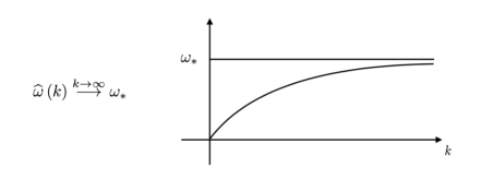
In this subsection we want to investigate the behavior at infinity of the dispersion curves that are bounded i.e. that have horizontal asymptote. Thus, let be a bounded solution of the equation . Under the assumption that this function is monotonically increasing in , setting
it is straightforward to show that admit a horizontal asymptote whose value is . Thanks to the particular expression of the function we can find a necessary (and computable) condition on both in the general relaxed micromorphic case and in the internal variable model. Indeed, in the general case it can be checked that the function is a polynomial of even order in the two variables , that can be written as
| (71) |
polynomial functions in . Our calculation gives that
In order to compare our relaxed model to the internal variable one (which is obtained setting ), we can regard the polynomials as functions of the three parameters and . Our calculation shows that the polynomials are zero for the following combinations of these three scalars:
| - | |
| - | |
| - | |
| - |
We can hence see that in the case of the internal variable model, the order of is smaller and
where the functions and are obtained from the setting .
Whit the purpose of clarify the general tool that we will find to calculate the horizontal asymptote of , we propose the following example.
Example 3.
Let us consider the polynomial
where we assume that are continuous. We look for solutions of
| (72) |
Dividing (72) by we have equivalently
| (73) |
Since
and
we obtain the necessary condition
| (74) |
The condition (74) is a necessary condition that the horizontal asymptote has to satisfy. Because in our situation we can not find an explicit expression for the dispersion curves, the only possibility that we have to calculate the values of the horizontal asymptote is to test the necessary condition (74). Adopting the notations proposed here, we can so finally prove the following
Proposition 4.
Let be a bounded solution of the problem with horizontal asymptote . Then .
Proof.
Being a solution of , we have i.e.
Dividing by we find
| (75) |
For the continuity of the functions we have
So passing to the limit in (75) we find
∎
Corollary 5.
If we have , and is a solution of the problem with horizontal asymptote , then .
Performing the calculation for the general relaxed micromorphic model and the internal variable one, and considering only the positive roots, we find the following possible values for the horizontal asymptotes
| (76) |
and
| (77) |
where
and
We set
Even if we leave not explicitly proven that the dispersion curves are monotonically increasing for all values of the constitutive parameters, we checked that it is indeed the case for a large number of numerical values of the parameters respecting positive definiteness of the strain energy density. Moreover, for all the checked values of the parameters, the values of computed by setting the coefficient of the higher order of appearing in the polynomial (71) to be equal to zero, (see (76) for the relaxed micromorphic model and (77) for the internal variable one) are always seen to be the values of the horizontal asymptotes of the bounded dispersion curves. Hence, even if we do not have an explicit proof that setting (or for the internal variable model) is also a sufficient condition for horizontal asymptotes, this is indeed the case for all combinations of the parameters which are sensible to be interesting for applications. We explicitly remark that the horizontal asymptotes shown in (76) are those found for the relaxed micromorphic model with , while those shown in (77) are relative to the internal variable case . We notice that, as shown in [26], the horizontal asymptotes for the internal variable model significantly differ from those obtained with the full non-local model (with non-vanishing , and ). This means that the internal variable model is a pathological limit of the relaxed micromorphic model, in the sense that setting to zero , and drastically changes the asymptotic properties of the dispersion curves.
4.1.4 Tangents in 0 to the acoustic curves
Another very important geometric characteristics of the dispersion curves are the slopes at the origin of the acoustic branches. In this way we can also directly compare our relaxed model to classical isotropic linear elasticity. In the case that we are studying in this paper, the direct computation of these quantities, given the great complexity of the involved expressions, is impossible. Therefore we work with the implicit function theorem applied to the expression of the determinant equation. First of all, we remark that the matrix given in (49) cannot generate acoustic branches since (when131313If , having that , one of the uncoupled branches becomes acoustic. ). Thus the two independent acoustic branches are generated by the matrices and . The acoustic branches are those solutions of the equations
such that . It can be checked that, for all , the two independent acoustic curves and verify the identities
| (78) |
for every and , where are real scalar functions of the vector of material parameters of the model
| (79) |
In order to isolate the quantity , which is the slope of the acoustic curves in , we remark that
| (80) |
However, since we compute that , the latter relation does not give any condition on For this reason we perform also the second derivative (the calculations are given in Appendix 3) finding then
| (81) |
with
| (82) | ||||
| (83) | ||||
| (84) |
and
| (85) |
Recalling, the final expressions for the two slopes are
Remembering the basic relations in [1, 34] between our relaxed micromorphic parameters and that
| (87) |
the equations in (LABEL:eq:slopes) can be neatly written as
| (88) |
Based on this result we see that the tangents to the acoustic curves fully recover the format of classical isotropic linear elasticity, if the latter model is taken with parameters . This result should be compared with [27, eq. 8.13] where Mindlin also obtained the tangents of the transverse and longitudinal acoustic branches in 0. However, his results for the more general micromorphic model do not support the transparency of (88).
5 Action of the material parameters on the behavior of the dispersion curves
In the relaxed micromorphic model presented in this work, we have considered the splitting, following the Lie-Cartan decomposition of , of the micro-inertia and of the potential part related to . This allows us to separate the governing behavior of the deformation mechanisms associated to the pure deformation, the volumetric expansion and the rotation of the microstructure. In this way, we can directly explore how each of these deformation modes affects the behavior of the dispersion curves. In the following, we show how varying independently the material parameters and we can act on the behavior of the dispersion curves with more freedom with respect to the non-weighted relaxed micromorphic model presented in [25]. We have numerically solved the equation looking for solutions of the type which are curves of the considered medium. In this section we analyze the obtained solutions for different choices of the material parameters in order to highlight their effect on the behavior of the dispersion curves. The material parameters in Table 2 are those used in the simulations if not differently specified.
| 400 | 100 | 100 | 440 | |||
| MPa | MPa | MPa | MPa | mm |
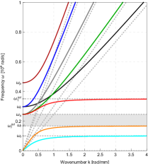
5.1 Classical results
Classical linear elasticity and the Cosserat model can be obtained as limit cases starting from the relaxed micromorphic one. In order to directly compare the dispersion curves of these models with those of the relaxed one, we present them in this sub-section. We briefly recall that the strain energy density for the classical linear elasticity is given by
Moreover, the kinetic energy density used for the classical model is clearly
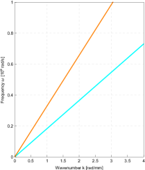
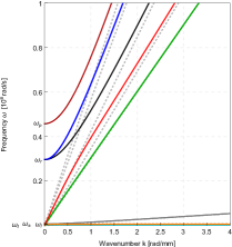
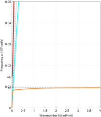
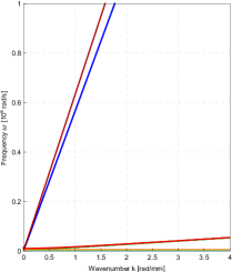
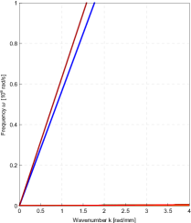
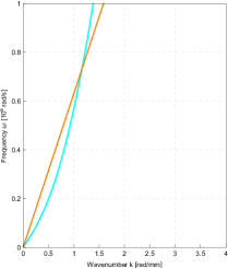
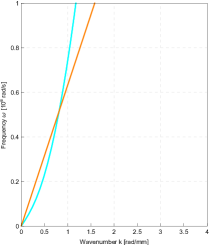
Classical Cauchy linear elasticity gives rise to the dispersion curves presented in Fig. 2 (left). The dispersion curves reduce to straight lines, which means that the speed of propagation of waves is independent of the frequency of the traveling waves. The slopes of the dispersion curves are given by for transversal waves and for longitudinal waves ( and are the Lamé parameters of the considered Cauchy continuum).
As for the weighted Cosserat model, it features a strain energy density of the type:
| (89) | ||||
where is constrained to be skew-symmetric. The kinetic energy considered for the Cosserat model takes the form:
| (90) |
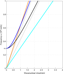
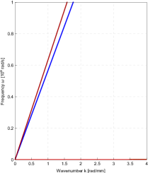
Following the same procedures shown in section 4 for the relaxed micromorphic model, the study of plane wave propagation in Cosserat media (we give the corresponding Euler-Lagrange equations in the appendix) gives rise to dispersion curves of the type shown in Fig.2 (right). The values of the asymptotes are given by
| (91) |
and for the values of the slopes of the acoustic branches we find
| (92) |
We will show in what follows that even if the Cosserat model allows to account for some dispersion at higher frequencies, the behavior of dispersion curves related to the relaxed micromorphic model is richer as it allows for the description of band-gaps and account for more complex microstructure motions. We will finally show that both the classical cases presented in this subsection (Cauchy and Cosserat) can be obtained as degenerate limit cases of the relaxed micromorphic model.
 |
 |
|
| (a) | (b) |
5.2 The classical relaxed micromorphic model and the internal variable model
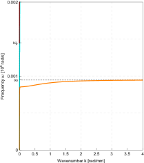
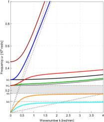
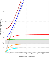
Before proceeding, we report some results already available in the literature [25, 26] which we obtain from our weighted model setting and (classical relaxed micromorphic case). Moreover, we also study the limit case that is obtained setting , which is also known as internal variable model (no derivatives of the micro-distortion appearing in the strain energy density). The dispersion curves for the two models are shown in Fig. 3.
 |
 |
 |
| (a1) longitudinal dispersion curves | (a2) transversal dispersion curves | (a3) uncoupled dispersion curves |
 |
 |
 |
| (b1) longitudinal dispersion curves | (b2) transversal dispersion curves | (b3) uncoupled dispersion curves |
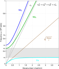
In both cases, we find 8 different dispersion curves instead of 12. Indeed, we would expect 12 curves since the kinematics is given by the 3 components of the displacement field , plus the 9 components of the micro-distortion field . This means that there are overlapped curves (our check exhibits 4 couples of overlapping curves). The band-gap region is clearly present in both models. These results are fully compatible with what has been found in [25] and in [26]. In particular, we find the same behavior presented in [25] and [26], where sufficient conditions on the constitutive parameters have been found that guarantee the existence of band gaps. Moreover, for the internal-variable case, it has been shown in [26] that two optic branches become horizontal and four horizontal asymptotes can be found which are not related with the two horizontal asymptotes of the case .
In the present work, in order to present a parametric study on the behavior of the dispersion curves varying a great number of material parameters, we have decided to represent, in the newly studied cases, all the dispersion curves in the same picture associating to every curve a specific color. With respect to the nomenclature states in [25] the correspondence with our choice of colors is as follows (Table 3):
| longitudinal curves | transversal curves | uncoupled curves | ||||||
|---|---|---|---|---|---|---|---|---|
| Dark Red | Blue | Black | ||||||
| Red | Green | Gray | ||||||
| Orange | Cyan | Gray |
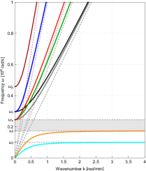
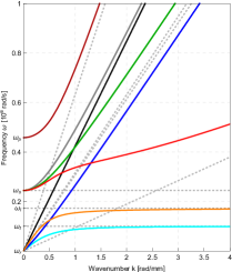
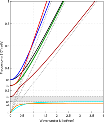
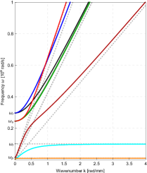
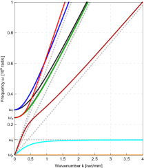
5.3 A panorama of dispersion curves for the weighted relaxed micromorphic model.
In this subsection we present a complete panorama of the dispersion curves associated to the weighted relaxed micromorphic model highlighting the effect of each of the weights and on the dispersion curves themselves. If not differently specified, the reference values of the weights are those given in the following table:
| - | - | - |
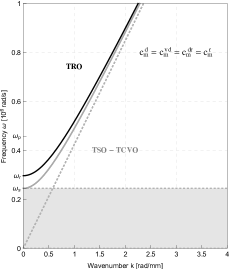
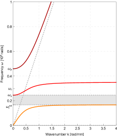
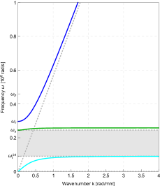
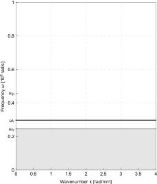
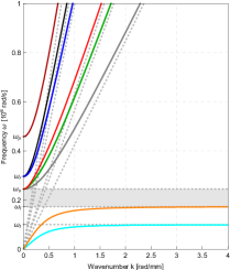
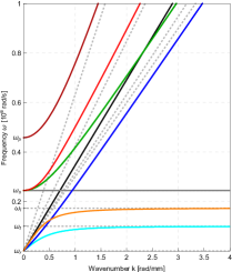
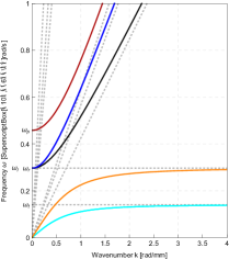
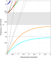
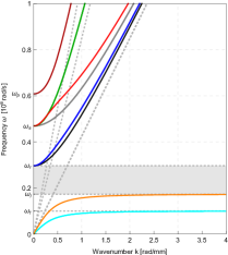
5.3.1 Case
Characteristic limit elastic energy .
Characteristic limit kinetic energy .
![[Uncaptioned image]](/html/1610.03296/assets/x10.png) |
![[Uncaptioned image]](/html/1610.03296/assets/x11.png) |
![[Uncaptioned image]](/html/1610.03296/assets/x12.png) |
 |
 |
 |
On the basis of the picture, it is clear that the action of the parameter preserves the presence of the band gap. This parameter does not act on the curves with a horizontal asymptote (cyan, orange) and it does not act on the optic curves in dark red and red. It is also possible to remark that with the variation of some curves change their oblique asymptotes. Finally, one of the dispersion curves becomes completely horizontal when setting . This feature is peculiar to the parameter because no completely horizontal curves are produced by setting or (see subsequent pictures). This means that it is mainly the parameter which governs non-localities in metamaterials. Indeed, horizontal dispersion curves are peculiar of metamaterials in which adjacent unit cells do not affect the behavior of each other based on the hypothesis of separation of scales (see [41, 39]). We explicitly remark that the picture obtained with is the one relative to the classical relaxed micromorphic model (see also Fig. 3 (a)).
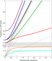
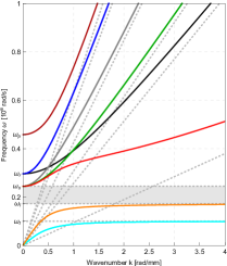
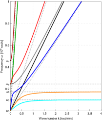
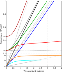
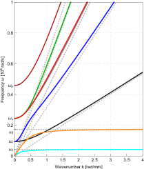
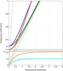
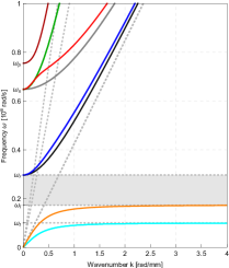
5.3.2 Case
Characteristic limit elastic energy .
Characteristic limit kinetic energy .
 |
 |
 |
 |
 |
 |
On the basis of the picture, it is clear that the action of the parameter preserves the presence of the band gap. Varying the values of this parameter, we have an action only on the curves in black and gray. The parameter is also seen to have some direct influence on the horizontal asymptotes for the orange optic wave. In fact if the value of this horizontal asymptote changes and we can calculate it solving the equation
| (93) |
with respect to . This is exactly the direct application of the proposition 4 in the case in which the coefficient is not present. Between the solutions of the eq.(93) we find
where
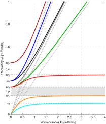
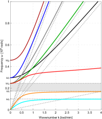
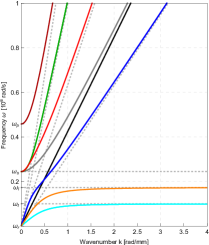
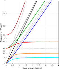
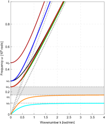
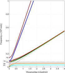
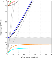
5.3.3 Case
Characteristic limit elastic energy
Characteristic limit kinetic energy .
![[Uncaptioned image]](/html/1610.03296/assets/x22.png) |
![[Uncaptioned image]](/html/1610.03296/assets/x23.png) |
![[Uncaptioned image]](/html/1610.03296/assets/x24.png) |
The action of the parameter preserves the presence of the band gaps. It acts only on the uncoupled curve in black leaving all the others fixed. The parameter has no direct effect neither on horizontal asymptotes, nor on the creation of purely horizontal curves.The oblique asymptote of the black branch is , and we explicitly remark that
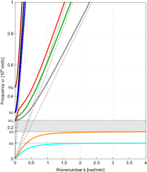
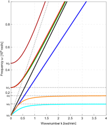
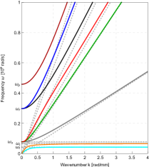
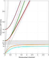
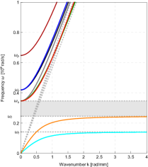
5.3.4 Case
Characteristic limit elastic energy .
Characteristic limit kinetic energy .
 |
 |
 |
 |
 |
 |
The combined action of the parameters and is given by the superposition of the effects observed in subsections 5.3.2 and 5.3.3. Only three curves (gray, orange, cyan) remain fixed.
5.3.5 Vanishing Cosserat couple modulus and
Characteristic limit elastic energy
Characteristic limit kinetic energy .
 |
 |
 |
 |
 |
 |
In this case we see that two curves (black and green) become acoustic. As a consequence, there is no complete band gap. This is coherent with the results of [25] in which the existence of 2 complete band-gaps is directly related to a non-vanishing Cosserat couple modulus . The particular effect of the parameter on the existence of a horizontal curve is preserved (see also Fig.4).
We explicitly mention that the presence of 4 acoustic curves is not observed in any known pattern of dispersion curves for real metamaterials. This means that such metamaterials need to have a non-vanishing Cosserat couple modulus which allows for the description of rotational micro-motions at higher frequencies.
5.3.6 Vanishing Cosserat couple modulus and
Characteristic limit elastic energy .
Characteristic limit kinetic energy .
 |
 |
 |
 |
 |
 |
Again, the two extra characteristic acoustic curves that arise when setting are recovered again. An effect of the parameter similar to the one shown in Fig. 5 is also found for the optic wave which becomes horizontal. A high value of has also a visible effect on one of the two extra acoustic curves.
5.3.7 Vanishing Cosserat couple modulus and
Characteristic limit elastic energy .
Characteristic limit kinetic energy .
![[Uncaptioned image]](/html/1610.03296/assets/x43.png) |
![[Uncaptioned image]](/html/1610.03296/assets/x44.png) |
![[Uncaptioned image]](/html/1610.03296/assets/x45.png) |
In this case we see again that two curves (blue and black) become acoustic. There is no complete band gap. This confirms once again the need of having as a necessary condition for the existence of complete band-gaps. The effect of the parameter is limited to the control of the slope of one of the two extra acoustic curves whose onset is related to the fact of setting .
5.4 Variation of the micro-inertia weighting
As shown in section 4.3.1, the three weights of the micro-inertia have a fundamental role on the definition of the cut-off frequencies of the optic waves. Indeed, this is one of the main results of the present paper: the split of the micro-inertia allows to control separately the starting point of the optic curves which can be translated along the y - axis by simply varying the value of each of the parameters . Such possibility of independent control of the optic branches is a major characteristic for an effective calibration of the material parameters of the relaxed micromorphic model on the dispersion patterns of real metamaterials.
5.4.1 Case
Characteristic limit elastic energy .
Characteristic limit kinetic energy .
 |
 |
 |
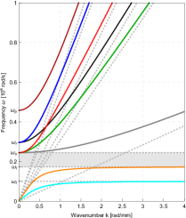
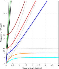
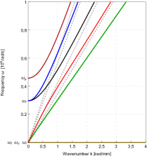
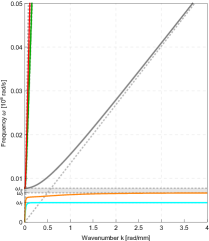
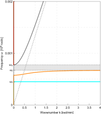
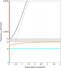
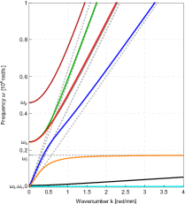
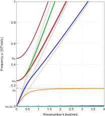
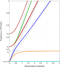
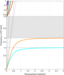
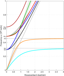
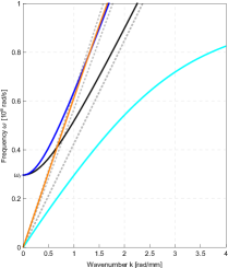
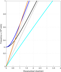
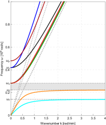
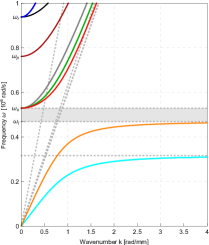
In this case we can see that the band gap is preserved when . For values the band gap is always present but it becomes smaller. For values of smaller than the behavior of the dispersion curves is unchanged with respect to the case with . This characteristic behavior is directly related to the definition of the cut-off frequency . For some of the optic branches go to infinity and do not appear in the dispersion diagram (Fig. 9 right). For smaller values of the optic branches starting from the cut-off frequency appear in the dispersion diagram (Fig. 9 center). For higher values of , the optic curves originating from start from a lower value and the slope of one of such curves becomes smaller (Fig. 9 right). In the limit one would expect that two optic branches related to become acoustic. This is indeed the case as it will be shown in subsection 5.4.5.
5.4.2 Case
Characteristic limit elastic energy .
Characteristic limit kinetic energy .
 |
 |
 |
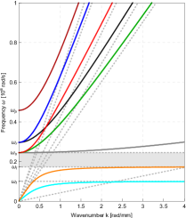
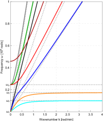
In this case we can see that the band gap is preserved when . There is a value such that for every the band gap is absent. This critical value can be related to the definition of the cut-off frequency .
Analogous consideration can be made with respect to the preceding case. In the present case the optic branches originating from are involved in the translations of the cut-offs associated to the variation of . The limit case will be discussed in subsection 5.4.6.
5.4.3 Case
Characteristic limit elastic energy .
Characteristic limit kinetic energy .
 |
 |
 |
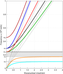
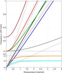
In this case we can see that the band gap is preserved when . We will see in section 5.4.7 that there is a value such that for every the band gap is absent. A similar behavior with respect to the previous two cases is observed for what concerns the optic wave originating from . The limit case will be described in section 5.4.7.
5.4.4 Cases : the fundamental role of the micro-inertia for enriched continuum mechanics
Characteristic limit elastic energy .
Characteristic limit kinetic energy .
 |
 |
 |
 |
 |
 |
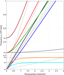
In Figure 12 we show the combined effect of the micro-inertia parameters on the behavior of the dispersion curves. When letting the three parameters tend to zero with the same speed, one ends up with a dispersion diagram which is peculiar of the classical linear elastic Cauchy media (Fig.12 bottom right).
This is a fundamental result of the present study which is not exhaustively treated in the literature: if one considers a continuum with enriched kinematic (), if no micro-inertia is considered to complement the macro-inertia , then the dispersion curves will not be different from those of the classical Cauchy continuum (Fig. 2 (a)). In order to activate the micro-motions associated to the micro-distortion tensor a micro-inertia is needed.
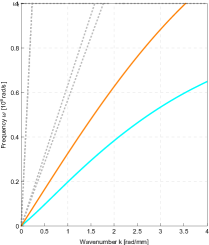
5.4.5 Case
Characteristic limit elastic energy .
Characteristic limit kinetic energy .
 |
 |
 |
We complete here the case treated in subsection 3.4.1, by describing the behavior of the dispersion curves when letting .
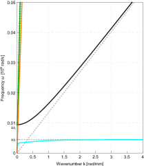
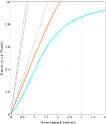
As expected, the optic branches originating from the cut-off become acoustic and, moreover, they are non-dispersive. What is more surprising is that the original acoustic branches flatten to zero and hence disappear from the dispersion diagram.
This means that, in the limit, we are constraining the system to have less degrees of freedom by artificially imposing an infinite inertia that does not allow some specific micro-vibrations.
 |
 |
 |
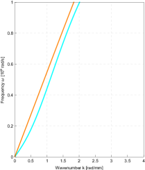
In Fig. 14 we make a zoom on the acoustic curves that are flattening to zero.
5.4.6 Case
Characteristic limit elastic energy .
Characteristic limit kinetic energy .
 |
 |
 |
The same reasoning of subsection 5.4.5 can be repeated here for the two optic curves originating from the cut-off .
 |
 |
 |
In Fig. 16 we show again the zoom on the dispersion curves that are flattening to zero.
5.4.7 Case
Characteristic limit elastic energy .
Characteristic limit kinetic energy .
 |
 |
 |
The same reasoning of subsection 5.4.5 can be repeated here for the two optic curves originating from the cut-off .
 |
 |
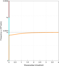 |
Fig. 18 shows the behavior of the dispersion curves flattening to zero.
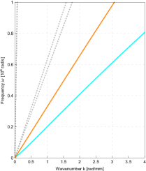
5.4.8 Cases : a rigidified Cauchy material
Characteristic limit elastic energy .
Characteristic limit kinetic energy .
 |
 |
 |
This particular case, obtained letting simultaneously and tend to infinity, gives rise to a Cauchy-like material behavior. Nevertheless, the physical meaning attached to this phenomenon is drastically different from the result obtained in section 5.4.4 when setting
Indeed, in that case, considering an enriched kinematics without the micro-inertia did not allow to such microstructure to manifest itself. It is as if one introduces a complex constitutive behavior for a metamaterial, but does not allow to investigate its dynamical behavior. Indeed, the result was the same obtained for the classical Cauchy medium as if it did not have any underlying microstructure.
On the other hand, the case considered here is quite different: we are indeed introducing the inertia of the microstructure in the model, but such inertia is so high that the microstructure is “frozen” and cannot vibrate locally. We thus end-up with a Cauchy material which is more rigid than the original one (slope of the acoustic curves is bigger than that in Fig. 1(a)).
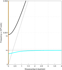
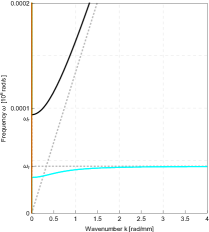
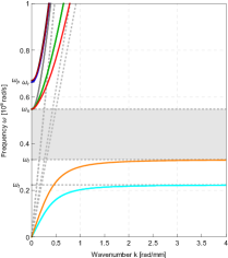
Case (internal variable model)
Characteristic limit elastic energy .
Characteristic limit kinetic energy .
 |
 |
 |
The band gap is always present. Nevertheless two curves become horizontal and 4 horizontal asymptotes instead of 2 are found letting . When two band-gaps can be created increasing the value of .
5.5 Other interesting cases
5.5.1 Case and decreasing
 |
 |
 |
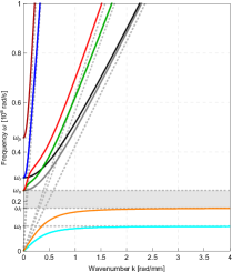
The effect of letting preserves the presence of the band-gap because it does not influence the acoustic branches and the cut-off sending instead the other two cut-offs to infinity.
5.5.2 Case
 |
 |
 |
5.5.3 Case “Cosserat limit”
 |
 |
 |
The effect of letting is equivalent to let . This means that only the skew-symmetric part of the micro-distortion tensor remains both in the elastic and kinetic energies that thus tend to the Cosserat energies given in eqs. (89) and (90).
It is clearly seen from Fig. 23 that an increasing value of directly acts on the acoustic dispersion curves which become straight lines. Moreover, the optic curves originating from and disappear from the dispersion diagrams since the two cut-offs tend to infinity. If we compare this limit case with the Cosserat model that we have given in (2) we can remark a perfect concordance.
5.5.4 Case “indeterminate couple stress theory”
Letting is equivalent to set and and . The corresponding strain energy density gives rise to the so called indeterminate couple stress model [36, 29]: since there are no degrees of freedom related to that remain active, the kinematics reduces to the simple displacement field. For this reason the term related to the micro-distortion in the kinetic energy must be neglected by setting .
 |
 |
 |
 |
 |
 |
As expected, and as it is known for second gradient theories, only two acoustic curves are found as it was the case for classical elasticity. The only extra feature with respect to the classical elasticity is that higher gradient models may account for some dispersive effects. In order to have a direct comparison with the indeterminate couple stress model, we have directly implement the indeterminate couple stress model considering the deformation energy (the relative strong equations can be found in the appendix)
With the same choice of the material parameters, we obtain the following dispersion curves:
 |
Conclusion
In this paper we present for the first time the “weighted” relaxed micromorphic model, by introducing the Cartan-Lie decomposition of the second order tensors and in the kinetic and elastic energies, respectively. It is found that the split of the tensor in the micro-inertia provides a unique feature to the model, namely the possibility of separately controlling the cut-offs of the optic curves in the dispersion diagram. This is an essential feature in view of the calibration of the relaxed micromorphic parameters on real band-gap metamaterials. The split of the second order tensor presents some effects on the dispersion curves which are less clearly related to possible physical situations. In general, we can say that the term governs, to a large extent, the non-locality in the considered metamaterials since it is able to give rise to a horizontal optic curve. On the other hand, the term is able to grant the onset of (extra) horizontal asymptotes for some optic curves. No specific effect can be attributed to the term .
Another important result of the present paper is that of showing the fundamental role of micro-inertia terms when dealing with enriched continua. It is shown that both the cases and give rise to a Cauchy-type situation in which only 2 straight acoustic branches can be recognized. Nevertheless, the physical meaning associated to such two cases is completely different. Indeed, setting in a model with enriched kinematics can be considered to be a mistake since one gives a complex and rich behavior to the elastic energy (through a particular dependence on ), but one does not allow the exploitation of such constitutive behavior due to the absence of the associated micro-inertia. It is hence not astonishing that, no matter how complex is the constitutive choice for the elastic energy (Mindlin, relaxed micromorphic, Cauchy, second gradient, etc.), the resulting dispersion curves are basically those of classical elasticity: two straight lines starting from the origin. The problem is simply that we do not give to the model the possibility to express its dynamical behavior since there is no micro-inertia that is able to trigger micro-vibrations.
On the other hand, the case is phenomenologically different: we introduce the micro-inertia in the model, but it is so “high” that the microstructure is “frozen” and this results in Cauchy-like materials. We leave to a forthcoming paper the task of studying in greater detail the importance of the role of micro-inertia in enriched continuum mechanics. Finally, some parametric studies on all of the introduced constitutive parameters are performed, thus giving a complete panorama of all possible dispersion patterns which are attainable in the relaxed micromorphic framework.
6 Acknowledgments
Angela Madeo thanks INSA-Lyon for the funding of the BQR 2016 "Caractérisation mécanique inverse des métamatériaux: modélisation, identification expérimentale des paramètres et évolutions possibles", as well as the CNRS-INSIS for the funding of the PEPS project.
7 Appendix
7.1 Variation of the kinetic energy
In order to derive the Euler-Lagrange equations, we need to assume a stronger regularity for the kinematical fields:
Having that
the action functional is Fréchet differentiable (and so Gâteaux differentiable) on the affine subspace
Its differential141414 is the vector space of admissible variations (test functions). at a point
evaluated at the admissible variation , is given by the variation of the part associated to the kinetic energy
and of that associated to the potential energy
We compute here the part of the action functional associated to the kinetic energy:
In order to find the Euler-Lagrange equations, we have to integrate by parts, with respect to the time derivative, the four parts :
Considering that
| (94) |
we find that
So considering only the bulk part , we have
7.2 Variation of the part of the potential energy
Remembering (4), the first variation of the action functional is computed thanks to the following identities:
| (95) | ||||
7.3 Derivation of PDEs in the new variables
The following identities will be useful in the following.
| (96) | ||||
We set
| (97) |
Equations in
This set of equations can be rewrite as follows:
| (98) | ||||
Remembering the definitions of given in (20),(21),(22), the scalar components of this vectorial system are therefore
| (99) | ||||
Thanks to the hypothesis of dependence only on , we have that are zero and . Thus the first equation of (99) becomes
Dividing by and remembering the definition of given in (LABEL:eq:asintoti_obliqui) we can rewrite this equation as:
| (100) |
Repeating the same calculation for the other two equations, and remembering the definition of and given in (LABEL:eq:asintoti_obliqui) and (LABEL:eq:omega), we find
| (101) |
Equations in
The PDEs system
| (102) | ||||
has only five independent equations. Setting for the system (102) of PDEs, the five independent equations that we will take are and In order to find the desired PDEs, we need the following calculations: we have
| (103) | ||||
where is defined in (97), and remembering that for every we find
For the trace we find
| (104) |
Equation 1
We have
Thus the first equation is
and remembering the definitions of and given in (LABEL:eq:omega) and (LABEL:eq:asintoti_obliqui) we find
| (105) |
Equations 2,3
| (106) | ||||
We have to calculate the term :
So we have
| (107) | ||||
Equation 4
| (108) | ||||
We have to calculate the term :
Thus we have
| (109) |
Equation 5
We have to determine So
and
Thus, for we find
| (110) |
and having that
| (111) | ||||
Thus we have
| (112) |
Equations in
The PDEs system
has only three independent equations.
Equations 1,2
| (113) | ||||
we have to calculate the term :
So we have
Equation 3
| (114) |
We have to calculate the term :
So we have
Equations in the spherical part of
7.4 Determination of slopes of the acoustic branches
We want to evaluate the first and second derivative in 0 of the expressions
with . In order to work with a more readable notation, in what follows we suppress the dependence by and of the relative functions. The derivative of with respect to is denoted by . We have
and so, remembering that , this condition does not give any information on the value of . For this reason, we continue with the second derivative. We compute separately the derivative of the four terms of the first derivative of obtaining:
Thus
| (115) |
Solving the equations (115) we find
and so, considering only the positive roots,
7.5 Derivation of strong equations for the Cosserat model and indeterminate couple stress model
In this appendix we give the strong field equations for the Cosserat model and the indeterminate couple stress model.
Cosserat model
The potential weighted energy for the Cosserat model is the following
| (116) | ||||
The first variation is computed exactly in the same way as in (11), giving the following system of PDEs:
| (117) | ||||
The system of PDEs (117) is not really suitable for the numerical implementation. Working only with the skew symmetric part of the micro-distortion tensor , it is more convenient to see like a vector thanks to the identification of the Lie algebra with by means of the axl-operator. In this way we can work only with the six independent equations of the system (117). We remember that for
the operator is defined as follows:
Thanks to the identities [37]
verified for every , the system of PDEs (117) can be rewritten in a completely equivalent form as
Indeterminate couple stress model
The potential weighted energy for the indeterminate couple stress model is the following [14]
| (118) | ||||
The first variation of this energy density gives the following system of PDEs:
The problem can be completely reformulated in terms of the gradient of the skew symmetric part of . Indeed, thanks to the equivalence
the following energy density
| (119) | ||||
is completely equivalent to (118). The associated system of Euler- Lagrange equations is
where anti is the inverse operator of axl defined as follows
References
- [1] Gabriele Barbagallo, Marco Valerio d’Agostino, Rafael Abreu, Ionel-Dumitrel Ghiba, Angela Madeo, and Patrizio Neff. Transparent anisotropy for the relaxed micromorphic model: macroscopic consistency conditions and long wave length asymptotics. arXiv preprint arXiv:1601.03667, to appear in Int. J. Solids Struct., 2016.
- [2] VL Berdichevskii and LI Sedov. Dynamic theory of continuously distributed dislocations. its relation to plasticity theory:vol. 31, no. 6, 1967, pp. 981–1000. Journal of Applied Mathematics and Mechanics, 31(6):989–1006, 1967.
- [3] Mircea Birsan and Patrizio Neff. On the dislocation density tensor in the Cosserat theory of elastic shells. arXiv preprint arXiv:1602.03421, 2016.
- [4] William D. Claus and Ahmed Cemal Eringen. Three dislocation concepts and micromorphic mechanics. Developments in Mechanics, 6:349–358, 1969.
- [5] William D. Claus and Ahmed Cemal Eringen. Dislocation dispersion of elastic waves. International Journal of Engineering Science, 9(7):605–610, 1971.
- [6] NM Cordero, Anais Gaubert, Samuel Forest, Esteban P Busso, F Gallerneau, and S Kruch. Size effects in generalised continuum crystal plasticity for two-phase laminates. Journal of the Mechanics and Physics of Solids, 58(11):1963–1994, 2010.
- [7] François Ebobisse, Klaus Hackl, and Patrizio Neff. A canonical rate-independent model of geometrically linear isotropic gradient plasticity with isotropic hardening and plastic spin accounting for the burgers vector. arXiv preprint arXiv:1603.00271, 2016.
- [8] François Ebobisse and Patrizio Neff. Existence and uniqueness for rate-independent infinitesimal gradient plasticity with isotropic hardening and plastic spin. Mathematics and Mechanics of Solids, 15(6):691–703, 2010.
- [9] François Ebobisse, Patrizio Neff, and Daya Reddy. Existence results in dislocation based rate-independent isotropic gradient plasticity with kinematical hardening and plastic spin: The case with symmetric local backstress. arXiv preprint arXiv:1504.01973, 2015.
- [10] Ahmed Cemal Eringen. Microcontinuum field theories: I. Foundations and Solids. Springer Science & Business Media, 2012.
- [11] Ahmed Cemal Eringen and William D. Claus. A micromorphic approach to dislocation theory and its relation to several existing theories. Technical report, DTIC Document, 1969.
- [12] Samuel Forest. Micromorphic approach for gradient elasticity, viscoplasticity, and damage. Journal of Engineering Mechanics, 135(3):117–131, 2009.
- [13] Samuel Forest. Nonlinear regularization operators as derived from the micromorphic approach to gradient elasticity, viscoplasticity and damage. In Proc. R. Soc. A, volume 472. The Royal Society, 2016.
- [14] Ionel-Dumitrel Ghiba, Patrizio Neff, Angela Madeo, and Ingo Münch. A variant of the linear isotropic indeterminate couple-stress model with symmetric local force-stress, symmetric nonlocal force-stress, symmetric couple-stresses and orthogonal boundary conditions. Mathematics and Mechanics of Solids, page 1081286515625535, 2016.
- [15] Ionel-Dumitrel Ghiba, Patrizio Neff, Angela Madeo, Luca Placidi, and Giuseppe Rosi. The relaxed linear micromorphic continuum: existence, uniqueness and continuous dependence in dynamics. Mathematics and Mechanics of Solids, 20(10):1171–1197, 2015.
- [16] Elena F. Grekova. Linear reduced Cosserat medium with spherical tensor of inertia, where rotations are not observed in experiment. Mechanics of Solids, 47(5):538–543, 2012.
- [17] Ekkehart Kröner. Discussion on papers by A.C. Eringen and W.D. Claus, Jr, and N. Fox. Fundamental Aspects of Dislocation Theory, 1:1054–1059.
- [18] MA Kulesh, Elena F. Grekova, and IN Shardakov. The problem of surface wave propagation in a reduced Cosserat medium. Acoustical Physics, 55(2):218–226, 2009.
- [19] Angela Madeo, Gabriele Barbagallo, Marco Valerio D’Agostino, Rafael Abreu, Ionel-Dumitrel Ghiba, and Patrizio Neff. Real wave propagation in the isotropic relaxed micromorphic model. accepted Proc. R. Soc. A, 2016.
- [20] Angela Madeo, Gabriele Barbagallo, Marco Valerio d’Agostino, Luca Placidi, and Patrizio Neff. First evidence of non-locality in real band-gap metamaterials: determining parameters in the relaxed micromorphic model. In Proc. R. Soc. A, volume 472, page 20160169. The Royal Society, 2016.
- [21] Angela Madeo, Patrizio Neff, Elias C Aifantis, Gabriele Barbagallo, and Marco Valerio d’Agostino. On the role of micro-inertia in enriched continuum mechanics. arXiv preprint arXiv:1607.07385, 2016.
- [22] Angela Madeo, Patrizio Neff, Gabriele Barbagallo, Marco Valerio d’Agostino, and Ionel-Dumitrel Ghiba. A review on wave propagation modeling in band-gap metamaterials via enriched continuum models. arXiv preprint arXiv:1609.01073, 2016.
- [23] Angela Madeo, Patrizio Neff, Marco Valerio d’Agostino, and Gabriele Barbagallo. Complete band gaps including non-local effects occur only in the relaxed micromorphic model. arXiv preprint arXiv:1602.04315, 2016.
- [24] Angela Madeo, Patrizio Neff, I-D Ghiba, Luca Placidi, and Giuseppe Rosi. Band gaps in the relaxed linear micromorphic continuum. Zeitschrift für Angewandte Mathematik und Mechanik, 95(9):880–887, 2015.
- [25] Angela Madeo, Patrizio Neff, Ionel-Dumitrel Ghiba, Luca Placidi, and Giuseppe Rosi. Wave propagation in relaxed micromorphic continua: modeling metamaterials with frequency band-gaps. Continuum Mechanics and Thermodynamics, 27(4-5):551–570, 2015.
- [26] Angela Madeo, Patrizio Neff, Ionel-Dumitrel Ghiba, and Giuseppe Rosi. Reflection and transmission of elastic waves in non-local band-gap metamaterials: A comprehensive study via the relaxed micromorphic model. Journal of the Mechanics and Physics of Solids, 95:441 – 479, 2016.
- [27] Raymond David Mindlin. Microstructure in linear elasticity. Technical report, Office of Naval Research, 1963.
- [28] Raymond David Mindlin. Micro-structure in linear elasticity. Archive for Rational Mechanics and Analysis, 16(1):51–78, 1964.
- [29] Ingo Münch and Patrizio Neff. A nonlinear micropolar continuum theory for initial plasticity. Advances and Trends in Structural Engineering, Mechanics and Computation, pages 269–272, 2010.
- [30] Patrizio Neff. On material constants for micromorphic continua. Trends in Applications of Mathematics to Mechanics, STAMM Proceedings, Seeheim, pages 337–348, 2004.
- [31] Patrizio Neff. Existence of minimizers for a finite-strain micromorphic elastic solid. Proceedings of the Royal Society of Edinburgh: Section A Mathematics, 136(05):997–1012, 2006.
- [32] Patrizio Neff. Existence of minimizers in nonlinear elastostatics of micromorphic solids. In Encyclopedia of Thermal Stresses, pages 1475–1485. Springer, 2014.
- [33] Patrizio Neff, Krzysztof Chełmiński, and Hans-Dieter Alber. Notes on strain gradient plasticity: finite strain covariant modelling and global existence in the infinitesimal rate-independent case. Mathematical Models and Methods in Applied Sciences, 19(02):307–346, 2009.
- [34] Patrizio Neff and Samuel Forest. A geometrically exact micromorphic model for elastic metallic foams accounting for affine microstructure. modelling, existence of minimizers, identification of moduli and computational results. Journal of Elasticity, 87(2-3):239–276, 2007.
- [35] Patrizio Neff, Ionel-Dumitrel Ghiba, Markus Lazar, and Angela Madeo. The relaxed linear micromorphic continuum: well-posedness of the static problem and relations to the gauge theory of dislocations. The Quarterly Journal of Mechanics and Applied Mathematics, pages 53–84, 2015.
- [36] Patrizio Neff, Ionel-Dumitrel Ghiba, Angela Madeo, Luca Placidi, and Giuseppe Rosi. A unifying perspective: the relaxed linear micromorphic continuum. Continuum Mechanics and Thermodynamics, 26(5):639–681, 2014.
- [37] Patrizio Neff and Ingo Münch. Curl bounds grad on so (3). ESAIM: Control, Optimisation and Calculus of Variations, 14(1):148–159, 2008.
- [38] Sergiy Nesenenko and Patrizio Neff. Well-posedness for dislocation based gradient viscoplasticity i: Subdifferential case. SIAM Journal on Mathematical Analysis, 44(3):1694–1712, 2012.
- [39] Kim Pham, Varvara G. Kouznetsova, and Marc G. D. Geers. Transient computational homogenization for heterogeneous materials under dynamic excitation. Journal of the Mechanics and Physics of Solids, 61(11):2125–2146, 2013.
- [40] Valentin L. Popov. Dynamics of plastic rotations in a medium with dislocations and disclinations. Technical Physics Letters, 20:576–577, 1994.
- [41] Ashwin Sridhar, Varvara G. Kouznetsova, and Marc G.D. Geers. Homogenization of locally resonant acoustic metamaterials towards an emergent enriched continuum. Computational Mechanics, 57(3):423–435, 2016.
- [42] Bob Svendsen, Patrizio Neff, and Andreas Menzel. On constitutive and configurational aspects of models for gradient continua with microstructure. Zeitschrift für Angewandte Mathematik und Mechanik, 89(8):687–697, 2009.