Inference for empirical Wasserstein distances on finite spaces

Abstract

The Wasserstein distance is an attractive tool for data analysis but statistical inference is hindered by the lack of distributional limits. To overcome this obstacle, for probability measures supported on finitely many points, we derive the asymptotic distribution of empirical Wasserstein distances as the optimal value of a linear program with random objective function. This facilitates statistical inference (e.g. confidence intervals for sample based Wasserstein distances) in large generality. Our proof is based on directional Hadamard differentiability. Failure of the classical bootstrap and alternatives are discussed. The utility of the distributional results is illustrated on two data sets.

Keywords: optimal transport, Wasserstein distance, central limit theorem, directional Hadamard derivative, bootstrap, hypothesis testing

AMS 2010 Subject Classification: Primary: 62G20, 62G10, 65C60 Secondary: 90C08, 90C31

1 Introduction

The Wasserstein distance (Vasershtein, , 1969), also known as Mallows distance (Mallows, , 1972), Monge-Kantorovich-Rubinstein distance in the physical sciences (Kantorovich and Rubinstein, , 1958; Rachev, , 1985; Jordan et al., , 1998), earth-mover’s distance in computer science (Rubner et al., , 2000) or optimal transport distance in optimization (Ambrosio, , 2003), is one of the most fundamental metrics on the space of probability measures. Besides its prominence in probability (e.g. Dobrushin, (1970); Gray, (1988)) and finance (e.g. Rachev and Rüschendorf, (1998)) it has deep connections to the asymptotic theory of PDEs of diffusion type (Otto, (2001), Villani, (2003, 2008) and references therein). In a statistical setting it has mainly been used as a tool to prove weak convergence in the context of limit laws (e.g. Bickel and Freedman, (1981); Shorack and Wellner, (1986); Johnson and Samworth, (2005); Dümbgen et al., (2011); Dorea and Ferreira, (2012)) as it metrizes weak convergence together with convergence of moments. However, recently the empirical (i.e. estimated from data) Wasserstein distance has also been recognized as a central quantity itself in many applications, among them clinical trials (Munk and Czado, , 1998; Freitag et al., , 2007), metagenomics (Evans and Matsen, , 2012), medical imaging (Ruttenberg et al., , 2013), goodness-of-fit testing (Freitag and Munk, , 2005; Del Barrio et al., , 1999), biomedical engineering (Oudre et al., , 2012), computer vision (Gangbo and McCann, , 2000; Ni et al., , 2009), cell biology (Orlova et al., , 2016) and model validation (Halder and Bhattacharya, , 2011). The barycenter with respect to the Wasserstein metric (Agueh and Carlier, , 2011) has been shown to elicit important structure from complex data and to be a promising tool, for example in deformable models (Boissard et al., , 2015; Agulló-Antolín et al., , 2015). It has also been used in large-scale Bayesian inference to combine posterior distributions from subsets of the data (Srivastava et al., , 2015).

Generally speaking three characteristics of the Wasserstein distance make it particularly attractive for various applications. First, it incorporates a ground distance on the space in question. This often makes it more adequate than competing metrics such as total-variation or $\chi^{2}$-metrics which are oblivious to any metric or similarity structure on the ground space. As an example, the success of the Wasserstein distance in metagenomics applications can largely be attributed to this fact (see Evans and Matsen, (2012) and also our application in Section 3.3).

Second, it has a clear and intuitive interpretation as the amount of ’work’ required to transform one probability distribution into another and the resulting transport can be visualized (see Section 3.2). This is also interesting in applications where probability distributions are used to represent actual physical mass and spatio-temporal changes have to be tracked.

Third, it is well-established (Rubner et al., , 2000) that the Wasserstein distance performs exceptionally well at capturing human perception of similarity. This motivates its popularity in computer vision and related fields.

Despite these advantages, the use of the empirical Wasserstein distance in a statistically rigorous way is severely hampered by a lack of inferential tools. We argue that this issue stems from considering too large classes of candidate distributions (e.g. those which are absolutely continuous with respect to the Lebesgue measure if the ground space has dimension $\geq 2$). In this paper, we therefore discuss the Wasserstein distance on finite spaces, which allows to solve this issue. We argue that the restriction to finite spaces is not merely an approximation to the truth, but rather that this setting is sufficient for many practical situations as measures often already come naturally discretized (e.g. two- or three-dimensional images - see also our applications in Section 3).

We remark that from our methodology further inferential procedures can be derived, e.g. a (M)ANOVA type of analysis and multiple comparisons of Wasserstein distances based on their $p$-values (see e.g. Benjamini and Hochberg, (1995)). Our techniques also extend immediately to dependent samples $(X_{i},Y_{i})$ with marginals $\bm{r}$ and $\bm{s}$.

Wasserstein distance

Let $(\mathcal{X},d)$ be a complete metric space with metric $d:\mathcal{X}\times\mathcal{X}\rightarrow\mathbb{R}_{\geq 0}$. The Wasserstein distance of order $p$ ($p\geq 1$) between two Borel probability measures $\mu_{1}$ and $\mu_{2}$ on $\mathcal{X}$ is defined as

$$W_{p}(\mu_{1},\mu_{2})=\left\{\inf_{\nu\in\Pi(\mu_{1},\mu_{2})}\int_{\mathcal{X}\times\mathcal{X}}d^{p}\!(x,x^{\prime})\nu(dx,dx^{\prime})\right\}^{1/p},$$

where $\Pi(\mu_{1},\mu_{2})$ is the set of all Borel probability measures on $\mathcal{X}\times\mathcal{X}$ with marginals $\mu_{1}$ and $\mu_{2}$, respectively.

Wasserstein distance on finite spaces

If we restrict in the above definition $\mathcal{X}=\left\{x_{1},\dots,x_{N}\right\}$ to be a finite space, every probability measure on $\mathcal{X}$ is given by a vector $\bm{r}$ in $\mathcal{P}_{\mathcal{X}}=\left\{\bm{r}=(r_{x})_{x\in\mathcal{X}}\in\mathbb{R}_{>0}^{\mathcal{X}}:\sum_{x\in\mathcal{X}}r_{x}=1\right\}$, via $P_{\bm{r}}(\{x\})=r_{x}$. We will not distinguish between the vector $\bm{r}$ and the measure it defines. The Wasserstein distance of order $p$ between two finitely supported probability measures $\bm{r},\bm{s}\in\mathcal{P}_{\mathcal{X}}$ then becomes

(1) $$W_{p}(\bm{r},\bm{s})=\left\{\min_{\bm{w}\in\Pi(\bm{r},\bm{s})}\sum_{x,x^{\prime}\in\mathcal{X}}d^{p}\!(x,x^{\prime})w_{x,x^{\prime}}\right\}^{1/p},$$

where $\Pi(\bm{r},\bm{s})$ is the set of all probability measures on $\mathcal{X}\times\mathcal{X}$ with marginal distributions $\bm{r}$ and $\bm{s}$, respectively. All our methods and results concern this Wasserstein distance on finite spaces.

1.1 Overview of main results

Distributional limits

The basis for inferential procedures for the Wasserstein distance on finite spaces is a limit theorem for its empirical version $W_{p}(\hat{\bm{r}}_{n},\hat{\bm{s}}_{m})$. Here, the empirical measure generated by independent random variables $X_{1},\dots,X_{n}\sim\bm{r}$ is given by $\hat{\bm{r}}_{n}=(\hat{r}_{n,x})_{x\in\mathcal{X}}$, where $\hat{r}_{n,x}=\frac{1}{n}\#\left\{k:X_{k}=x\right\}$. Let $\hat{\bm{s}}_{m}$ be generated from i.i.d. $Y_{1},\dots,Y_{m}\sim\bm{s}$ in the same fashion. Under the null hypothesis $\bm{r}=\bm{s}$ we prove that

(2) $$\left(\frac{nm}{n+m}\right)^{\frac{1}{2p}}W_{p}(\hat{\bm{r}}_{n},\hat{\bm{s}}_{m})\Rightarrow\left\{\max_{{\bm{u}}\in\Phi^{*}_{p}}\langle\bm{G},{\bm{u}}\rangle\right\}^{\frac{1}{p}},\quad n,m\rightarrow\infty.$$

Here, ’$\Rightarrow$’ means convergence in distribution, $\bm{G}$ is a mean zero Gaussian random vector with covariance depending on $\bm{r}=\bm{s}$ and $\Phi_{p}^{*}$ is the convex set of dual solutions to the Wasserstein problem depending on the metric $d$ only (see Theorem 1). In Section 3.2 we use this result to assess the statistical significance of the differences between real and synthetically generated fingerprints in the Fingerprint Verification Competition (Maio et al., , 2002).

We give analogous results under the alternative $\bm{r}\neq\bm{s}$. This extends the scope of our results beyond the classical two-sample (or goodness-of-fit test) as it allows for confidence statements on $W_{p}(\bm{r},\bm{s})$ when the null hypothesis of equality is likely or even known to be false. An example for this is given by our application to metagenomics (Section 3.3) where samples from the same person taken at different times are typically statistically different but our asymptotic results allow us to assert with statistical significance that inter-personal distances are larger that intra-personal ones.

Proof strategy

We prove these results by showing that the Wasserstein distance is directionally Hadamard differentiable (Shapiro, , 1990) and the right hand side of (2) is its derivative evaluated at the Gaussian limit of the empirical multinomial process (see Theorem 4). This notion generalizes Hadamard differentiability by allowing non-linear derivatives but still allows for a refined delta-method (Römisch, (2004) and Theorem 3). Notably, the Wasserstein distance is not Hadamard differentiable in the usual sense.

Explicit limiting distribution for tree metrics

When the space $\mathcal{X}$ are the vertices of a tree and the metric $d$ is given by path length we give an explicit expression for the limiting distribution in (2) (see Theorem 5). In contrast to the general case, this explicit formula allows for fast and direct simulation of the limiting distribution. This extends a previous result of Samworth and Johnson, (2004) who considered a finite number of point masses on the real line. The Wasserstein distance on trees has, to the best of our knowledge, only been considered in two papers: Kloeckner, (2013) studies the geometric properties of the Wasserstein space of measures on a tree and Evans and Matsen, (2012) use the Wasserstein distance on phylogenetic trees to compare microbial communities.

The bootstrap

Directional Hadamard differentiability is not enough to guarantee the consistency of the naive ($n$ out of $n$) bootstrap (Dümbgen, , 1993; Fang and Santos, , 2014) - in contrast to the usual notion of Hadamard differentiability. This implies that the bootstrap is not consistent for the Wasserstein distance (1)(see Theorem 6). In contrast, the $m$-out-of-$n$ bootstrap for $m/n\rightarrow 0$ is known to be consistent in this setting (Dümbgen, , 1993) and can be applied to the Wasserstein distance. Under the null hypothesis $\bm{r}=\bm{s}$, however, there is a more direct way of obtaining an approximation of the limiting distribution. In the appendix, we discuss this alternative re-sampling scheme based on ideas of Fang and Santos, (2014), that essentially consists of plugging in a bootstrap version of the underlying empirical process in the derivative. We show that this scheme, which we will call directional bootstrap, is consistent for the Wasserstein distance (see Theorem 6, Section B).

1.2 Related work

Empirical Wasserstein distances

In very general terms, we study a particular case (finite spaces) of the following question and its two-sample analog: Given the empirical measure $\mu_{n}$ based on $n$ i.i.d. random variables taking variables in a metric space with law $\mu$. What can be inferred about $W_{p}(\mu_{n},\mu_{0})$ for a reference measure $\mu_{0}$ which may be equal to $\mu$?

It is a well-known and straightforward consequence of the strong law of large numbers that if the $p$-th moments are finite for $\mu$ and $\mu_{0}$ then $W_{p}(\mu_{n},\mu_{0})$ converges to $W_{p}(\mu,\mu_{0})$, almost surely, as the sample size $n$ approaches infinity (Villani, , 2008, Cor. 6.11). Determining the exact rate of this convergence is the subject of an impressive body of literature developed over the last decades starting with the seminal work of Ajtai et al., (1984) considering for $\mu_{0}$ the uniform distribution on the unit square, followed by Talagrand, (1992, 1994) for the uniform distribution in higher dimensions and Horowitz and Karandikar, (1994) giving bounds on mean rates of convergence. Boissard and Gouic, (2014); Fournier and Guillin, (2014) gave general deviation inequalities for the empirical Wasserstein distance on metric spaces. For a discussion in the light of our distributional limit results see Section 4.

Distributional limits give a natural perspective for practicable inference, but despite considerable interest in the topic have remained elusive to a large extent. For measures on $\mathcal{X}=\mathbb{R}$ a rather complete theory is available (see Munk and Czado, (1998); Freitag et al., (2007); Freitag and Munk, (2005) for $\mu_{0}\neq\mu$ and e.g. Del Barrio et al., (1999); Samworth and Johnson, (2005); Del Barrio et al., (2005) for $\mu_{0}=\mu$ as well as Mason, (2016); Bobkov and Ledoux, (2014) for recent surveys). However, for $\mathcal{X}=\mathbb{R}^{d}$, $d\geq 2$ the only distributional result known to us is due to Rippl et al., (2015) for specific multivariate (elliptic) parametric classes of distributions, when the empirical measure is replaced by a parametric estimate. In the context of deformable models distributional results are proven (Del Barrio et al., , 2015) for specific multidimensional parametric models which factor into one-dimensional parts.

The simple reason why the Wasserstein distance is so much easier to handle in the one-dimensional case is that in this case the optimal coupling attaining the infimum in (1) is known explicitly. In fact, the Wasserstein distance of order $p$ between two measures on $\mathbb{R}$ then becomes the $L^{p}$ norm of the difference of their quantile functions (see Mallows, (1972) for an early reference) and the analysis of empirical Wasserstein distances can be based on quantile process theory. Beyond this case, explicit coupling results are only known for multivariate Gaussians and elliptic distributions (Gelbrich, , 1990). A classical result of Ajtai et al., (1984) for the uniform distribution on $\mathcal{X}=[0,1]^{2}$ suggests that, even in this simple case, distributional limits will have a complicated form if they exist at all. We will elaborate on this thought in the discussion, in Section 4.

The Wasserstein distance on finite spaces has been considered recently by Gozlan et al., (2013) to derive entropy inequalities on graphs and by Erbar and Maas, (2012) to define Ricci curvature for Markov chains on discrete spaces. To the best of our knowledge, empirical Wasserstein distances on finite spaces have only been considered by Samworth and Johnson, (2004) in the special case of measures supported on $\mathbb{R}$. We will show (Section 2.5) that our results extend theirs.

Directional Hadamard differentiability

We prove our distributional limit theorems using the theory of parametric programming (Bonnans and Shapiro, , 2013) which investigates how the optimal value and the optimal solutions of an optimization problem change when the objective function and the constraints are changed. While differentiability properties of optimal values of linear programs are extremely well studied such results have, to the best of our knowledge, not yet been applied to the statistical analysis of Wasserstein distances.

It is well-known that under certain conditions the optimal value of a mathematical program is differentiable with respect to the constraints of the problem (Rockafellar, , 1984; Gal et al., , 1997). However, the derivative will typically be non-linear. The appropriate concept for this is directional Hadamard differentiability (Shapiro, , 1990). The derivative of the optimal value of a mathematical program is typically again given as an extremal value.

Although the delta-method for directional Hadamard derivatives has been known for a long time (Shapiro, , 1991; Dümbgen, , 1993), this notion scarcely appears in the statistical context (with some exceptions, such as Römisch, (2004), see also Donoho and Liu, (1988)). Recently, an interest in the topic has evolved in econometrics (see Fang and Santos, (2014) and references therein).

Organization of the paper

In Section 2 we give a comprehensive result on distributional limits for the Wasserstein distance for measures supported on finitely many points. In Section 3 we apply our methods to two data sets to highlight different aspects. In Section 4 we briefly address limitations and possible extensions of our work. In the supplementary Material we discuss the bootstrap for the Wasserstein distance and give some technical proofs.

2 Distributional limits

2.1 Main result

In this section we give a comprehensive result on distributional limits for the Wasserstein distance when the underlying population measures are supported on finitely many points $\mathcal{X}=\left\{x_{1},\dots,x_{N}\right\}$. We denote the inner product on the vector space $\mathbb{R}^{\mathcal{X}}$ by $\langle{\bm{u}},{\bm{u}}^{\prime}\rangle=\sum_{x\in\mathcal{X}}u_{x}u^{\prime}_{x}$ for ${\bm{u}},{\bm{u}}^{\prime}\in\mathbb{R}^{\mathcal{X}}$.

Theorem 1.

Let $p\geq 1$, $\bm{r},\bm{s}\in\mathcal{P}_{\mathcal{X}}$ and $\hat{\bm{r}}_{n},\hat{\bm{s}}_{m}$ generated by i.i.d. samples $X_{1},\dots,X_{n}\sim\bm{r}$ and $Y_{1},\dots,Y_{m}\sim\bm{s}$, respectively. We define the convex sets

(3) $$\begin{split}\Phi^{*}_{p}&=\left\{{\bm{u}}\in\mathbb{R}^{\mathcal{X}}:u_{x}-u_{x^{\prime}}\leq d^{p}(x,x^{\prime}),\quad x,x^{\prime}\in\mathcal{X}\right\}\\ \Phi^{*}_{p}(\bm{r},\bm{s})&=\left\{({\bm{u}},\bm{v})\in\mathbb{R}^{\mathcal{X}}\times\mathbb{R}^{\mathcal{X}}:\begin{split}&\langle{\bm{u}},\bm{r}\rangle+\langle\bm{v},\bm{s}\rangle=W_{p}^{p}(\bm{r},\bm{s}),\\ &u_{x}+v_{x^{\prime}}\leq d^{p}(x,x^{\prime}),\>x,x^{\prime}\in\mathcal{X}\end{split}\right\}\end{split}$$

and the multinomial covariance matrix

(4) $$\Sigma(\bm{r})=\begin{bmatrix}r_{x_{1}}(1-r_{x_{1}})&-r_{x_{1}}r_{x_{2}}&\cdots&-r_{x_{1}}r_{x_{N}}\\ -r_{x_{2}}r_{x_{1}}&r_{x_{2}}(1-r_{x_{2}})&\cdots&-r_{x_{2}}r_{x_{N}}\\ \vdots&&\ddots&\vdots\\ -r_{x_{N}}r_{x_{1}}&-r_{x_{N}}r_{x_{2}}&\cdots&r_{x_{N}}(1-r_{x_{N}})\end{bmatrix}$$

such that with independent Gaussian random variables $\bm{G}\sim\mathcal{N}(0,\Sigma(\bm{r}))$ and $\bm{H}\sim\mathcal{N}(0,\Sigma(\bm{s}))$ we have the following.

1. (One sample - Null hypothesis) With the sample size $n$ approaching infinity, we have the weak convergence

   (5) $$n^{\frac{1}{2p}}W_{p}(\hat{\bm{r}}_{n},\bm{r})\Rightarrow\left\{\max_{{\bm{u}}\in\Phi^{*}_{p}}\langle\bm{G},{\bm{u}}\rangle\right\}^{\frac{1}{p}}.$$

2. (One sample - Alternative) With $n$ approaching infinity we have

   (6) $$n^{\frac{1}{2}}\left(W_{p}(\hat{\bm{r}}_{n},\bm{s})-W_{p}(\bm{r},\bm{s})\right)\Rightarrow\frac{1}{p}W_{p}^{1-p}(\bm{r},\bm{s})\left\{\max_{({\bm{u}},\bm{v})\in\Phi_{p}^{*}(\bm{r},\bm{s})}\langle\bm{G},{\bm{u}}\rangle\right\}.$$

3. (Two samples - Null hypothesis) Let $\rho_{n,m}=\left(nm/(n+m)\right)^{1/2}$. If $\bm{r}=\bm{s}$ and $n$ and $m$ are approaching infinity such that $n\wedge m\rightarrow\infty$ and $m/(n+m)\rightarrow\lambda\in(0,1)$ we have

   (7) $$\rho_{n,m}^{1/p}W_{p}(\hat{\bm{r}}_{n},\hat{\bm{s}}_{m})\Rightarrow\left\{\max_{{\bm{u}}\in\Phi_{p}^{*}}\langle\bm{G},{\bm{u}}\rangle\right\}^{\frac{1}{p}}.$$

4. (Two samples - Alternative) With $n$ and $m$ approaching infinity such that $n\wedge m\rightarrow\infty$ and $m/(n+m)\rightarrow\lambda\in[0,1]$

   (8) $$\begin{split}\rho_{n,m}&\left(W_{p}(\hat{\bm{r}}_{n},\hat{\bm{s}}_{m})-W_{p}(\bm{r},\bm{s})\right)\Rightarrow\\ &\frac{1}{p}W_{p}^{1-p}(\bm{r},\bm{s})\left\{\max_{({\bm{u}},\bm{v})\in\Phi_{p}^{*}(\bm{r},\bm{s})}\sqrt{\lambda}\langle\bm{G},{\bm{u}}\rangle+\sqrt{1-\lambda}\langle\bm{H},\bm{v}\rangle\right\}.\end{split}$$

The sets $\Phi_{p}^{*}$ and $\Phi_{p}^{*}(\bm{r},\bm{s})$ are (derived from) the dual solutions to the Wasserstein linear program (see Theorem 4 below). This result is valid for all probability measures with finite support, regardless of the (dimension of the) underlying space. In particular, it generalizes a result of Samworth and Johnson, (2004), who considered a finite collection of point masses on the real line and $p=2$. We will re-obtain their result as a special case in Section 2.5 when we give explicit expressions for the limit distribution when the metric $d$, which enters the limit law via the dual solutions $\Phi_{p}^{*}$ or $\Phi_{p}^{*}(\bm{r},\bm{s})$, is given by a tree.

Remark 1.

In our numerical experiments (see Section 3 we have found the representation (8) to be numerically unstable when used to simulate from the limiting distribution under the alternative. We therefore give an alternative representation (18) in the supplementary material as a one-dimensional optimization problem of a non-linear function (in contrast to a high-dimensional linear program shown here). Note that the limiting distribution under the null does not suffer from this problem and can be simulated from directly using a linear program solver.

The scaling rate in Theorem 1 depends solely on $p$ and is completely independent of the underlying space $\mathcal{X}$. This contrasts known bounds on the rate of convergence in the continuous case. We will elaborate on the differences in the discussion. Typical choices are $p=1,2$. The faster scaling rate can be a reason to favor $p=1$. In our numerical experiments however, this advantage was frequently outweighed by larger quantiles of the limiting distribution.

Dümbgen, (1993) showed that the naive $n$-out-of-$n$ bootstrap is inconsistent for functionals with a non-linear Hadamard derivative, but resampling fewer than $n$ observations leads to a consistent bootstrap. Since we will show in the following that the Wasserstein distance belongs to this class of functionals, it is a direct consequence that the naive bootstrap fails for the Wasserstein distance (see Section B in the supplementary material for details) and that the following holds.

Theorem 2.

Let $\hat{\bm{r}}_{n}^{*}$ and $\hat{\bm{s}}_{m}^{*}$ be bootstrap versions of $\hat{\bm{r}}_{n}$ and $\hat{\bm{s}}_{m}$ that are obtained via re-sampling $k$ observations with $k/n\rightarrow 0$ and $k/m\rightarrow 0$. Then, the plug-in bootstrap with $\hat{\bm{r}}_{n}^{*}$ and $\hat{\bm{s}}_{m}^{*}$ is consistent, that is

$$\begin{split}\sup_{f\in\mathrm{BL}_{1}(\mathbb{R})}E\left[f(\phi_{p}(\sqrt{k}\left\{(\hat{\bm{r}}_{n}^{**},\hat{\bm{s}}_{m}^{**})-(\hat{\bm{r}}_{n},\hat{\bm{s}}_{m})\right\}))|X_{1},\dots,X_{n},Y_{1},\dots,Y_{m}\right]\\ -E\left[f\left(\rho_{n,m}\left\{W_{p}^{p}(\hat{\bm{r}}_{n},\hat{\bm{s}}_{m})-W_{p}^{p}(\bm{r},\bm{s})\right\}\right)\right]\end{split}$$

converges to zero in probability.

In the following we will prove our main Theorem 1 by

1. introducing Hadamard directional differentiability, which does not require the derivative to be linear but still allows for a delta-method;

2. showing that the map $(\bm{r},\bm{s})\mapsto W_{p}(\bm{r},\bm{s})$ is differentiable in this sense.

2.2 Hadamard directional derivatives

In this section we follow Römisch, (2004). A map $f$ defined on a subset $D_{f}\subset\mathbb{R}^{d}$ with values in $\mathbb{R}$ is called Hadamard directionally differentiable at ${\bm{u}}\in\mathbb{R}^{d}$ if there exists a map $f^{\prime}_{{\bm{u}}}:\mathbb{R}^{d}\rightarrow\mathbb{R}$ such that

(9) $$\lim_{n\rightarrow\infty}\frac{f({\bm{u}}+t_{n}\bm{h}_{n})-f({\bm{u}})}{t_{n}}=f^{\prime}_{\bm{u}}(\bm{h})$$

for any $\bm{h}\in\mathbb{R}^{d}$ and for arbitrary sequences $t_{n}$ converging to zero from above and $\bm{h}_{n}$ converging to $\bm{h}$ such that ${\bm{u}}+t_{n}\bm{h}_{n}\in D_{f}$ for all $n\in\mathbb{N}$. Note that in contrast to the usual notion of Hadamard differentiability (e.g. Van der Vaart and Wellner, (1996)) the derivative $\bm{h}\mapsto f^{\prime}_{\bm{u}}(\bm{h})$ is not required to be linear. A prototypical example is the absolute value $f:\mathbb{R}\rightarrow\mathbb{R}$, $t\mapsto|t|$ which is not in the usual sense Hadamard differentiable at $t=0$ but directionally differentiable with the non-linear derivative $t\mapsto|t|$.

Theorem 3 (Römisch, , 2004, Theorem 1).

Let $f$ be a function defined on a subset $F$ of $\mathbb{R}^{d}$ with values in $\mathbb{R}$, such that

1. $f$ is Hadamard directionally differentiable at ${\bm{u}}\in F$ with derivative $f^{\prime}_{\bm{u}}:F\rightarrow\mathbb{R}$ and

2. there is a sequence of $\mathbb{R}^{d}$-valued random variables $X_{n}$ and a sequence of non-negative numbers $\rho_{n}\rightarrow\infty$ such that $\rho_{n}(X_{n}-{\bm{u}})\Rightarrow X$ for some random variable $X$ taking values in $F$.

Then, $\rho_{n}(f(X_{n})-f({\bm{u}}))\Rightarrow f_{\bm{u}}^{\prime}(X)$.

2.3 Directional derivative of the Wasserstein distance

In this section we show that the functional $(\bm{r},\bm{s})\mapsto W_{p}^{p}(\bm{r},\bm{s})$ is Hadamard directionally differentiable and give a formula for the derivative.

The dual program (cf. (Luenberger and Ye, , 2008, Ch. 4), also Kantorovich and Rubinstein, (1958)) of the linear program defining the Wasserstein distance (1) is given by

(10) $$\begin{split}&\max_{({\bm{u}},\bm{v})\in\mathbb{R}^{\mathcal{X}}\times\mathbb{R}^{\mathcal{X}}}\quad\langle{\bm{u}},\bm{r}\rangle+\langle\bm{s},\bm{v}\rangle\\ \textbf{s.t.}\quad&u_{x}+v_{x^{\prime}}\leq d^{p}(x,x^{\prime})\quad\forall x,x^{\prime}\in\mathcal{X}.\end{split}$$

As noted above, the optimal value of the primal problem is $W_{p}^{p}(\bm{r},\bm{s})$ and by standard duality theory of linear programs (e.g. Luenberger and Ye, (2008)) this is also the optimal value of the dual problem. Therefore, the set of optimal solutions to the dual problem is given by $\Phi^{*}_{p}(\bm{r},\bm{s})$ as defined in (3).

Theorem 4.

The functional $(\bm{r},\bm{s})\mapsto W_{p}^{p}(\bm{r},\bm{s})$ is directionally Hadamard differentiable at all $(\bm{r},\bm{s})\in\mathcal{P}_{\mathcal{X}}\times\mathcal{P}_{\mathcal{X}}$ with derivative

(11) $$(\bm{h}_{1},\bm{h}_{2})\mapsto\max_{({\bm{u}},\bm{v})\in\Phi^{*}_{p}(\bm{r},\bm{s})}-(\langle{\bm{u}},\bm{h}_{1}\rangle+\langle\bm{v},\bm{h}_{2}\rangle).$$

We can give a more explicit expression for the set $\Phi^{*}_{p}(\bm{r},\bm{s})$ in the case $\bm{r}=\bm{s}$, when the optimal value of the primal and the dual problem is $0$. Then, the condition $W_{p}^{p}(\bm{r},\bm{s})=\langle\bm{r},{\bm{u}}\rangle+\langle\bm{s},\bm{v}\rangle$ becomes $\langle\bm{r},{\bm{u}}+\bm{v}\rangle=0$. Since $u_{x}+v_{x^{\prime}}\leq d^{p}\!(x,x^{\prime})$ for all $x,x^{\prime}\in\mathcal{X}$ implies ${\bm{u}}+\bm{v}\leq 0$ this yields ${\bm{u}}=-\bm{v}$. This gives

$$\Phi^{*}_{p}(\bm{r},\bm{r})=\left\{({\bm{u}},-{\bm{u}})\in\mathbb{R}^{\mathcal{X}}\times\mathbb{R}^{\mathcal{X}}:u_{x}-u_{x^{\prime}}\leq d^{p}\!(x,x^{\prime}),\>x,x^{\prime}\in\mathcal{X}\right\}$$

and the following more compact representation of the dual solutions in the case $\bm{r}=\bm{s}$, independent of $\bm{r}$:

(12) $$\Phi_{p}^{*}(\bm{r},\bm{r})=\Phi^{*}_{p}\times\left(-\Phi_{p}^{*}\right).$$

2.4 Proof of Theorem 1

1. With the notation introduced in Theorem 1, $n\hat{\bm{r}}_{n}$ is a sample of size $n$ from a multinomial distribution with probabilities $\bm{r}$. Therefore, $\sqrt{n}(\hat{\bm{r}}_{n}-\bm{r})\Rightarrow\bm{G}$ as $n\rightarrow\infty$ (Wasserman, , 2011, Thm. 14.6). The Hadamard derivative of the map $(\bm{r},\bm{s})\mapsto W_{p}^{p}(\bm{r},\bm{s})$ as given in Theorem 4 can now be used in the delta-method from Theorem 3. Together with the representation (12) of the set of dual solutions $\Phi^{*}_{p}(\bm{r},\bm{s})$, this yields

   $$\sqrt{n}W_{p}^{p}(\hat{\bm{r}}_{n},\bm{r})\Rightarrow\max_{({\bm{u}},\bm{v})\in\Phi^{*}_{p}(\bm{r},\bm{r})}-\langle{\bm{u}},\bm{G}\rangle\>\stackrel{{\scriptstyle D}}{{\sim}}\>\max_{{\bm{u}}\in\Phi^{*}_{p}}\langle{\bm{u}},\bm{G}\rangle.$$

   Here and in the following $Z_{1}\stackrel{{\scriptstyle D}}{{\sim}}Z_{2}$ means the distributional equality of the random variables $Z_{1}$ and $Z_{2}$. Applying to this the Continuous Mapping Theorem with the map $t\mapsto t^{1/p}$ gives the assertion.

2. Consider the map $(\bm{r},\bm{s})\mapsto W_{p}(\bm{r},\bm{s})=(W_{p}^{p}(\bm{r},\bm{s}))^{1/p}$. By Theorem 4 and the chain rule for Hadamard directional derivatives (Shapiro, , 1990, Prop. 3.6), the Hadamard derivative of this map at $(\bm{r},\bm{s})$ is given by

   (13) $$(\bm{h}_{1},\bm{h}_{2})\mapsto p^{-1}W_{p}^{1-p}(\bm{r},\bm{s})\left\{\max_{({\bm{u}},\bm{v})\in\Phi^{*}_{p}(\bm{r},\bm{s})}-(\langle{\bm{u}},\bm{h}_{1}\rangle+\langle\bm{v},\bm{h}_{2}\rangle)\right\}.$$

   An application of the delta-method of Theorem 3 concludes this part.

3. and d). Note that under the assumptions of the Theorem

   (14) $$\sqrt{\frac{nm}{n+m}}\left((\hat{\bm{r}}_{n},\hat{\bm{s}}_{m})-(\bm{r},\bm{s})\right)\Rightarrow(\sqrt{\lambda}\bm{G},\sqrt{1-\lambda}\bm{H}).$$

   Part d) follows with the delta-method from (13) and (14).

   For part c) we use, as we did for a), the derivative given in Theorem 4 and the Continuous Mapping Theorem. The limit distribution is

   $$\left\{\max_{({\bm{u}},\bm{v})\in\Phi^{*}_{p}(\bm{r},\bm{s})}(\sqrt{\lambda}\langle\bm{G},{\bm{u}}\rangle+\sqrt{1-\lambda}\langle\bm{H},\bm{v}\rangle)\right\}^{1/p}.$$

   Note that if $\bm{r}=\bm{s}$ we have $({\bm{u}},\bm{v})\in\Phi^{*}_{p}(\bm{r},\bm{s})$ if and only if ${\bm{u}}\in\Phi^{*}_{p}$ and $\bm{v}=-{\bm{u}}$, by (12) and (3). Hence, with $\bm{G}\stackrel{{\scriptstyle D}}{{\sim}}\bm{H}$ we conclude

   $$\begin{split}\max_{({\bm{u}},\bm{v})\in\Phi^{*}_{p}(\bm{r},\bm{s})}(\sqrt{\lambda}\langle\bm{G},{\bm{u}}\rangle+\sqrt{1-\lambda}\langle\bm{H},\bm{v}\rangle)&\stackrel{{\scriptstyle D}}{{\sim}}\max_{{\bm{u}}\in\Phi^{*}_{p}}(\sqrt{\lambda}\langle\bm{G},{\bm{u}}\rangle-\sqrt{1-\lambda}\langle\bm{H},{\bm{u}}\rangle)\\ &\stackrel{{\scriptstyle D}}{{\sim}}\max_{{\bm{u}}\in\Phi^{*}_{p}}\sqrt{\lambda+(1-\lambda)}\langle\bm{G},{\bm{u}}\rangle\\ &=\max_{{\bm{u}}\in\Phi^{*}_{p}}\langle\bm{G},{\bm{u}}\rangle.\end{split}$$

2.5 Explicit limiting distribution for tree metrics

Assume that the metric structure on $\mathcal{X}$ is given by a weighted tree, that is, an undirected connected graph $\mathcal{T}=(\mathcal{X},E)$ with vertices $\mathcal{X}$ and edges $E\subset\mathcal{X}\times\mathcal{X}$ that contains no cycles. We assume the edges to be weighted by a function $w:E\rightarrow\mathbb{R}_{>0}$. For $x,x^{\prime}\in\mathcal{X}$ let $e_{1},\dots,e_{l}\in E$ be the unique path in $\mathcal{T}$ joining $x$ and $x^{\prime}$, then the length of this path, $d_{\mathcal{T}}(x,x^{\prime})=\sum_{j=1}^{l}w(e_{j})$ defines a metric $d_{\mathcal{T}}$ on $\mathcal{X}$. Without imposing any further restriction on $\mathcal{T}$, we assume it to be rooted at $\mathrm{root}(\mathcal{T})\in\mathcal{X}$, say. Then, for $x\in\mathcal{X}$ and $x\neq\mathrm{root}(\mathcal{T})$ we may define $\mathrm{parent}(x)\in\mathcal{X}$ as the immediate neighbor of $x$ in the unique path connecting $x$ and $\mathrm{root}(\mathcal{T})$. We set $\mathrm{parent}(\mathrm{root}(\mathcal{T}))=\mathrm{root}(\mathcal{T})$. We also define $\mathrm{children}(x)$ as the set of vertices $x^{\prime}\in\mathcal{X}$ such that there exists a sequence $x^{\prime}=x_{1},\dots,x_{l}=x\in\mathcal{X}$ with $\mathrm{parent}(x_{j})=x_{j+1}$ for $j=1,\dots,l-1$. Note that with this definition $x\in\mathrm{children}(x)$. Additionally, define the linear operator $S_{\mathcal{T}}:\mathbb{R}^{\mathcal{X}}\rightarrow\mathbb{R}^{\mathcal{X}}$

$$(S_{\mathcal{T}}{\bm{u}})_{x}=\sum_{x^{\prime}\in\mathrm{children}(x)}u_{x^{\prime}}.$$

Theorem 5.

Let $p\geq 1$, $\bm{r}\in\mathcal{P}_{\mathcal{X}}$, defining a probability distribution on $\mathcal{X}$ and let the empirical measures $\hat{\bm{r}}_{n}$ and $\hat{\bm{s}}_{m}$ be generated by independent random variables $X_{1},\dots,X_{n}$ and $Y_{1},\dots Y_{m}$, respectively, all drawn from $\bm{r}=\bm{s}$.

Then, with a Gaussian vector $\bm{G}\sim\mathcal{N}(0,\Sigma(\bm{r}))$ as defined in (4) we have the following.

1. (One sample) As $n\rightarrow\infty$,

   (15) $$n^{\frac{1}{2p}}W_{p}(\hat{\bm{r}}_{n},\bm{r})\Rightarrow\left\{\sum_{x\in\mathcal{X}}|(S_{\mathcal{T}}\bm{G})_{x}|d_{\mathcal{T}}(x,\mathrm{parent}(x))^{p}\right\}^{\frac{1}{p}}$$

2. (Two samples) If $n\wedge m\rightarrow\infty$ and $n/(n+m)\rightarrow\lambda\in(0,1)$ we have

   (16) $$\left(\frac{nm}{n+m}\right)^{\frac{1}{2p}}W_{p}(\hat{\bm{r}}_{n},\hat{\bm{s}}_{m})\Rightarrow\left\{\sum_{x\in\mathcal{X}}|(S_{\mathcal{T}}\bm{G})_{x}|d_{\mathcal{T}}(x,\mathrm{parent}(x))^{p}\right\}^{\frac{1}{p}}.$$

The proof of Theorem 5 is given in the supplementary material. The theorem includes the special case of a discrete measure on the real line, that is $\mathcal{X}\subset\mathbb{R}$, since in this case, $\mathcal{X}$ can be regarded as a simple rooted tree consisting of only one branch.

Corollary 1 (Samworth and Johnson, , 2004, Theorem 2.6).

Let $\mathcal{X}=\{x_{1}<\dots<x_{N}\}\in\mathbb{R}$, $\bm{r}\in\mathcal{P}_{\mathcal{X}}$ and $\hat{\bm{r}}_{n}$ the empirical measure generated by i.i.d. random variables $X_{1},\dots,X_{n}\sim\bm{r}$. With $\bar{r}_{j}=\sum_{i=1}^{j}r_{x_{i}}$, for $j=1,\dots N$ and $B$ a standard Brownian bridge, we have as $n\rightarrow\infty$,

(17) $$n^{\frac{1}{4}}W_{2}(\hat{\bm{r}}_{n},\bm{r})\Rightarrow\left\{\sum_{j=1}^{N-1}|B(\bar{r}_{j})|(x_{j+1}-x_{j})^{2}\right\}^{\frac{1}{2}}.$$

3 Simulations and applications

The following numerical experiments were performed using R (R Core Team, , 2016). All computations of Wasserstein distances and optimal transport plans as well as their visualizations were performed with the R-package transport (Schuhmacher et al., , 2014; Gottschlich and Schuhmacher, , 2014). The code used for the computation of the limiting distributions is available as an R-package otinference (Sommerfeld, , 2017).

3.1 Speed of convergence

We investigate the speed of convergence to the limiting distribution in Theorem 1 in the one-sample case under the null hypothesis. To this end, we consider as ground space $\mathcal{X}$ a regular two-dimensional $L\times L$ grid with the euclidean distance as the metric $d$ and $L=3,5,10$. We generate five random measures $\bm{r}$ on $\mathcal{X}$ as realizations of a Dirichlet random variable with concentration parameter $\bm{\alpha}=(\alpha,\dots,\alpha)\in\mathbb{R}^{L\times L}$ for $\alpha=1,5,10$. Note, that $\alpha=1$ corresponds to a uniform distribution on the probability simplex. For each measure, we generate $20,000$ realizations of $n^{1/2p}W_{p}(\hat{\bm{r}}_{n},\bm{r})$ with $n\hat{\bm{r}}_{n}\sim\mathrm{Multinom}(\bm{r})$ for $n=10,1000,1000$ and of the theoretical limiting distribution given in Theorem 1. The Kolmogorov-Smirnov distance (that is, the maximum absolute difference between their cdfs) between these two samples (averaged over the five measures) is shown in Figure 1.

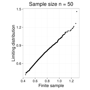
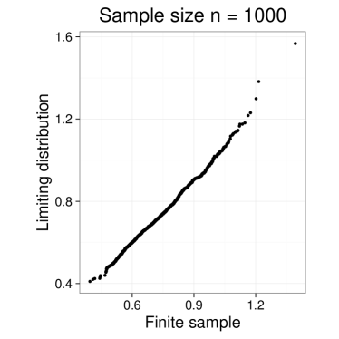
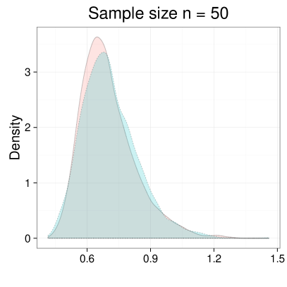
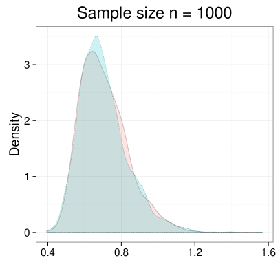
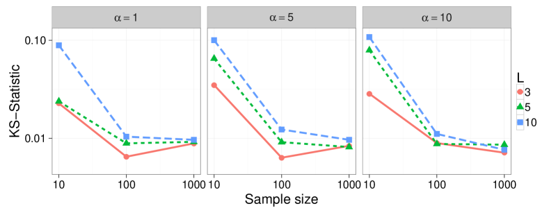
Figure 1: Comparison of the finite sample distribution and the theoretical limiting distribution on a regular grid of length $L$ for different sample sizes. The two top rows show Q-Q-plots and kernel density estimates (bandwidth: Silverman’s rule of thumb (Silverman, , 1986), solid line: finite sample, dotted line: limiting distribution) for $L=10$. Last row shows the KS statistic between the two distributions as a function of the sample size for different $L$ and for different concentration parameters $\alpha$.

The experiment shows that the limiting distribution is a good approximation of the finite sample version even for small sample sizes. For the considered parameters the size of the ground space $N=L^{2}$ seems to slow the convergence only marginally. Similarly, the underlying measure seems to have no sizeable effect on the convergence speed as the dependence on the concentration parameter $\alpha$ demonstrates.

3.2 Testing the null: real and synthetic fingerprints

The generation and recognition of synthetic fingerprints is a topic of great interest in forensic science and current state-of-the-art methods (Cappelli et al., , 2000) produce synthetic fingerprints that even human experts fail to recognize as such (Maltoni et al., , 2009, p. 292ff). Recently, Gottschlich and Huckemann, (2014) presented a method using the Wasserstein distance that is able to distinguish synthetic from real fingerprints with high accuracy. Their method is probabilistic in nature, since it is based on a hypothesized unknown distribution of certain features of the fingerprint. We use our distributional limits to assess the statistical significance of the differences.

Minutiae histograms

The basis for the comparison of fingerprints are so called minutiae which are key qualities in biometric identification based on fingerprints (Jain, , 2007). They are certain characteristic features such as bifurcations of the line patterns of the fingerprint. Each of the minutiae have a location in the fingerprint and a direction such that it can be characterized by two real numbers and an angle. Figure 3 shows a real and a synthetic fingerprint with their minutiae.

The recognition method of Gottschlich and Huckemann, (2014) considers pairs of minutiae and records their distance and the difference between their angles. Based on these two values each minutiae pair is put in one of 100 bins arranged in a regular grid (10 directional by 10 distance bins) to obtain a so called minutiae histogram (MH). Based on the bin-wise mean of MHs for several fingerprints to construct a typical MH, they found that the proximity in Wasserstein distance to these references is a good classifier for distinguishing real and synthetic fingerprints.

In order to assess the statistical significance of the difference in minutiae pair distributions, we consider fingerprints from the databases 1 and 4 of the Fingerprint Verification Competition of 2002 (Maio et al., , 2002), containing $110$ real and synthetic fingerprints, respectively. From each database the minutiae were obtained by automatic procedure using a commercial off-the-shelf program. For each fingerprint we chose disjoint minutiae pairs at random to avoid the issue of pairs being dependent yielding a total of 1917 and 1437 minutiae pairs from real and synthetic fingerprints, respectively.

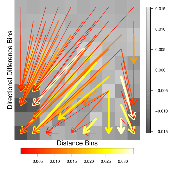
Figure 2: The optimal transport plan between the MHs of real and fake fingerprints. The grey values indicate the magnitude of the difference of the two MHs. The arrows show the transport. The amount of mass transported is encoded in the color and thickness of the arrows.

While two-sample tests for univariate data are abundant and well studied there are no multivariate methods that could be considered standard in this setting. Therefore, we report on the findings of several tests from the literature for comparison with the Wasserstein based method from (7). We tested the null hypothesis of the underlying distributions being equal for the un-centered, the centered and the centered and scaled (to variance $1$) data to assess effects beyond first moments using the following methods: 1) comparing the empirical Wasserstein distance $W_{1}$ after binning on a regular $10\times 10$ grid with the limiting distribution from Theorem 1; 2) a permutation test; 3) the crossmatch test proposed by (Rosenbaum, , 2005) and 4) the kernel based test (Anderson et al., , 1994) implemented in the R package ks.

Table 1 shows the resulting empirical distributions on a $10\times 10$ grid and the $p$-values for the different tests.

Table 1: Results of different two-sample tests for difference in the distribution of MHs of real and fake fingerprints.

	Wasserstein	Crossmatch	Permutation	KDE
Raw	0.00E+00	2.99E-01	1.00E-03	1.12E-08
Centered	4.00E-04	4.48E-05	1.00E-03	2.60E-21
Centered & Scaled	2.54E-02	1.01E-02	1.71E-01	1.79E-14

The differences are highly significant according to all tests, except the permutation test for the centered and scaled data. In this particular example at least, the Wasserstein based test seems to be able to pick up differences in distributions (in the first moment and beyond) at least as good as current state-of-the-art methods.

In addition to testing, the Wasserstein method provides us with an optimal transport plan, transforming one measure into the other. For the minutiae histograms under consideration this is illustrated in Figure 2. This transport plan gives information beyond a simple test for equality as it highlights structural changes in the distribution. In this specific application it reveals how in the minutiae histogram of synthetic fingerprints compared to the one of real fingerprints mass has been shifted from large and intermediate directional differences to smaller ones. In particular to small and large distances, and only to a lesser extent to intermediate distances. In conclusion one may say that synthetic fingerprints show smaller differences in the directions of minutiae and stronger clustering of minutiae distances around small and large values. Insight of this sort may lead to improved generation or detection of synthetic fingerprints.

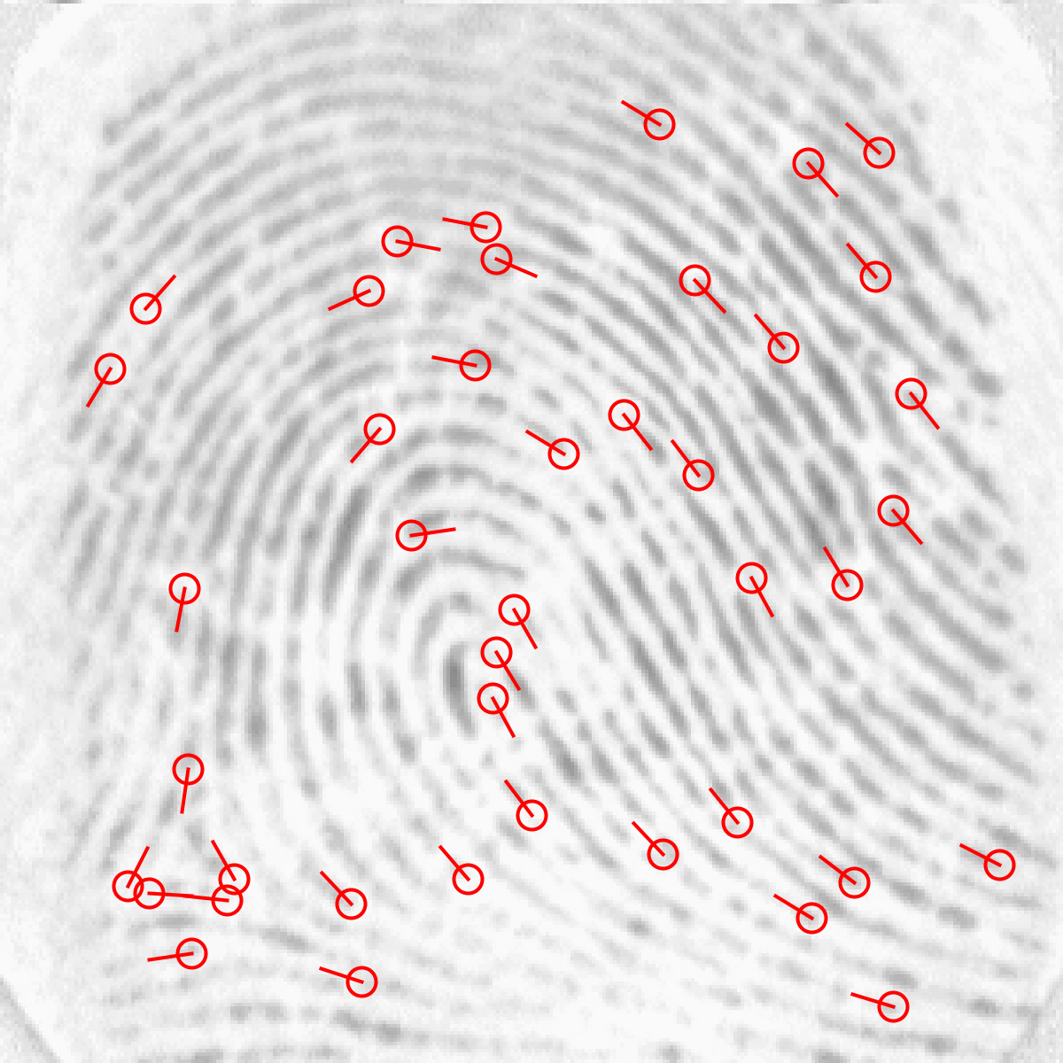
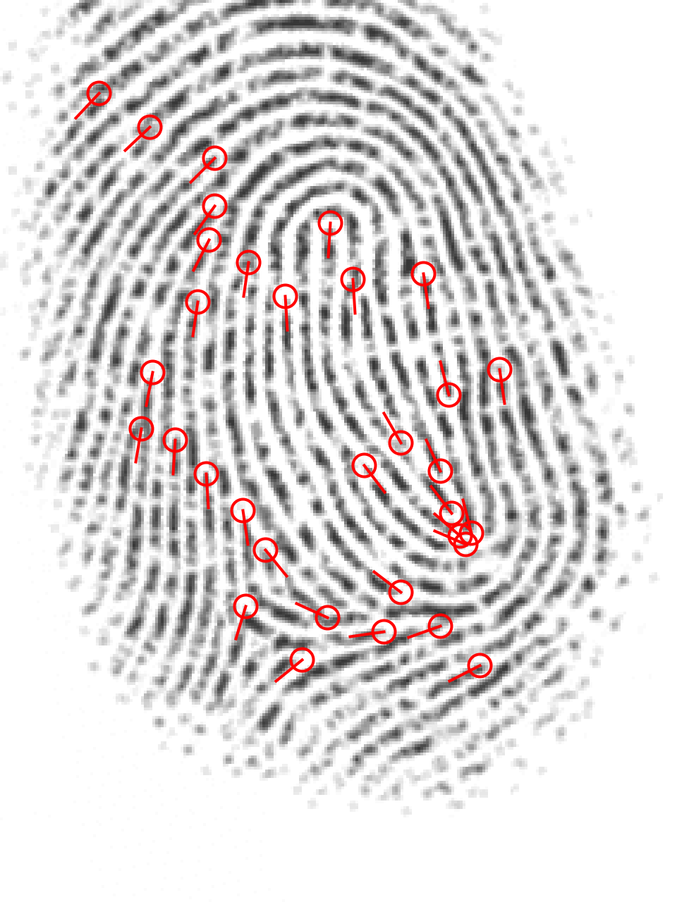
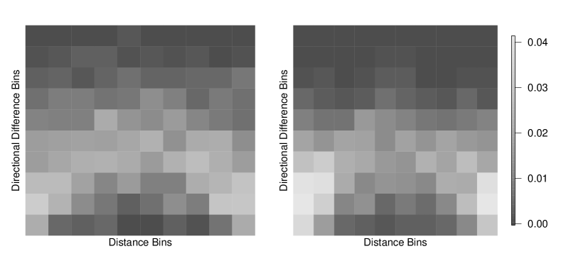
Figure 3: Top row: Minutiae of a real (left) and a synthetic (right) fingerprint. Bottom row: Minutiae histograms of real and synthetic fingerprints.

3.3 Asymptotic under the alternative: metagenomics

Figure 4: Relative abundances of the $30$ first OTUs in the $12$ samples (left) and Wasserstein distances of the microbial communities (right). Here, $ij$ is the $j$-th sample of the $i$-th person.

Metagenomics studies microbial communities by analyzing genetic material in an environmental sample such as a stool sample of a human. High-throughput sequencing techniques no longer require cultivated cloned microbial cultures to perform sequencing. Instead, a sample with potentially many different species can be analyzed directly and the abundance of each species in the sample can be recovered. The applications of this technique are countless and constantly growing. In particular, the composition of microbial communities in the human gut has been associated with obesity, inflammatory bowel disease and others (Turnbaugh et al., , 2007).

The analysis of a sample with high-throughput sequencing techniques yields several thousands to many hundreds of thousands sequences. After elaborate pre-processing, these sequences are aligned to a reference database and clustered in operational taxonomic units (OTUs). These OTUs can be thought of (albeit omitting some biological detail) as the different species present in the sample. For each OTU this analysis yields the number of sequences associated with it, that is how often this particular OTU was detected in the sample. Further, comparing the genetic sequences associated with an OTU yields a biologically meaningful measure of similarity between OTUs - and hence a distance. A metagenomic sample can therefore be regarded as a sample in a discrete metric space with OTUs being the points of the space. Comparing such samples representing microbial communities is of great interest (Kuczynski et al., , 2010). The Wasserstein distance has been recognized to provide valuable insight and to facilitate tests for equality of two communities (Evans and Matsen, , 2012). This previous application however, relies on a phylogenetic tree that is build on the OTUs and the distance is then measured in the tree. This additional pre-processing step involves many parameter choices and is unnecessary with our method.

A further drawback of the method of Evans and Matsen, (2012) is that it only allows for testing the null hypothesis of two communities being equal. In practice, one frequently finds that natural variation is so high that even two samples from the same source taken at different times will be recognized as different. This raises the question whether variation within samples from the same source is smaller than the difference to samples of another source. Statistically speaking we are looking for confidence sets for differences which are assumed to be different from zero. This requires asymptotics under the alternative $\bm{r}\neq\bm{s}$, which is provided by Theorem 1.

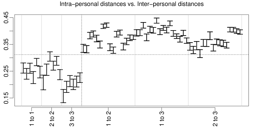
Figure 5: Display of $95\%$ confidence intervals of Wasserstein distances of microbial communities. The horizontal axis shows which person pair the distances belong to (separated by gray vertical lines). The dotted vertical line separates intra- (left) from inter- (right) -personal distances.

Data analysis

We consider part of the data of Costello et al., (2009). Four stool samples were taken from each of three persons at different times. We used the preparation of this data by P. Schloss available at https://www.mothur.org/w/images/d/d8/CostelloData.zip. The reads were pre-processed with the program mothur (Schloss et al., , 2009) using the procedure outlined in Schloss et al., (2011) and Schloss, (2015). The relative abundances of the $30$ most frequent OTUs and the Wasserstein-2 distances of the microbial communities are shown in Figure 4. In this and all other figures we use $i-j$ to denote sample $j$ of person $i$. Note that it is typical for this data that most of the mass is concentrated on a few OTUs.

The Wasserstein-2 distances for all $66$ pairs and their $99\%$ confidence intervals were computed using the asymptotic distribution in Theorem 1. The results are shown in Figure 5. The entire analysis took less than a minute on a standard laptop. The confidence intervals show that intra-personal distances are in fact significantly smaller than inter-personal distances.

4 Discussion

We discuss limitations, possible extensions of the presented work and promising directions for future research.

Beyond finite spaces I: rates in the finite and the continuous setting ($d=1$)

The scaling rate in Theorem 1 depends solely on $p$ and is completely independent of the underlying space $\mathcal{X}$. This contrasts known bounds on the rate of convergence in the continuous case (see references in the Introduction), which exhibit a strong dependence on the dimension of the space and the moments of the distribution.

Under the null hypothesis (that is, the two underlying population measures are equal) and when $\mathcal{X}=\mathbb{R}$ and $p=2$, the scaling rate for a continuous distribution is known to be $n^{1/2}$, at least under additional tail conditions (see e.g. Del Barrio et al., (2005)). This means that in this case the scaling rate for a discrete distribution is slower (namely $n^{1/4}$). Under the alternative (different population measures) the scaling rate is $n^{1/2}$ and coincide in the discrete and the continuous case (see Munk and Czado, (1998)).

Beyond finite spaces II: higher dimensions ($d\geq 2$)

For a continuous measure $\mu$ the Wasserstein distance is the solution of an infinite-dimensional optimization problem. Although differentiability results also exist for such problems (e.g. Shapiro, (1992)), there are strong indications that the argument presented here cannot carry over to the this case for $d\geq 2$. This is most easily seen from the classical results of Ajtai et al., (1984). We consider the uniform distribution on the unit square. For two samples of size $n$ independently drawn from this distribution, Ajtai et al., (1984) showed that there exist constants $C_{1},C_{2}$ such that the 1-Wasserstein distance $\hat{W}_{1}^{(n)}$ between them satisfies

$$C_{1}n^{-1/2}(\log n)^{1/2}\leq\hat{W}_{1}^{(n)}\leq C_{2}n^{-1/2}(\log n)^{1/2}$$

with probability $1-o(1)$. Hence, for $c_{n}\hat{W}_{1}^{(n)}$ to have a non-degenerate limit, we need $c_{n}=\sqrt{n/\log n}$. However, a common property of all delta-methods is that they preserve the rate of convergence, which is not satisfied here.

Transport distances on trees

Complementing our Theorem 5 a further result on transport distances on trees was proven by Evans and Matsen, (2012) in the context of phylogenetic trees for the comparison of metagenomic samples (see also our application in Section 3). They point out that the Wasserstein-1 distance on trees is equal to the so-called weighted uni-frac distance which is very popular in genetics. Inspired by this distance they give a formal generalization mimicking a cost exponent $p>1$ and consider its asymptotic behavior. However, as they remark, these generalized expressions are no longer related (beyond a formal resemblance) to Wasserstein distances with cost exponent $p>1$. Comparing the performance of their ad-hoc metric and the true Wasserstein distance on trees that is under consideration here is an interesting topic for further research.

Bootstrap

We showed that while the naive $n$-out-of-$n$ bootstrap fails for the Wasserstein distance (Section B), the $m$-out-of-$n$ bootstrap is consistent. An interesting and challenging question is how $m$ should be chosen.

Wasserstein barycenters

Barycenters in the Wasserstein space (Agueh and Carlier, , 2011) have recently received much attention (Cuturi and Doucet, , 2014; Del Barrio et al., , 2015). We expect that the techniques developed here can be of use in providing a rigorous statistical theory (e.g. distributional limits). The same applies to geodesic principal component analysis in the Wasserstein space (Bigot et al., , 2013; Seguy and Cuturi, , 2015).

Alternative cost matrices and transport distances

Theorem 1 holds in very large generality for arbitrary cost matrices, including in particular the case of a cost matrix derived from a metric but using a cost exponent $p<1$.

Beyond this obvious modification it seems worthwhile to extend the methodology of directional differentiability in conjunction with a delta-method to other functionals related to optimal transport, e.g. entropically regularized (Cuturi, , 2013) or sliced Wasserstein distances (Bonneel et al., , 2015). This would require a careful investigation of the analytical properties of these quantities similar to classical results for the Wasserstein distance.

Appendix A An alternative representation of the limiting distribution

We give a second representation of the limiting distribution under the alternative $\bm{r}\neq\bm{s}$. The random part of the limiting distribution (8) is the linear program

$$\max_{({\bm{u}},\bm{v})\in\Phi^{*}_{p}(\bm{r},\bm{s})}\sqrt{\lambda}\langle\bm{G},{\bm{u}}\rangle+\sqrt{1-\lambda}\langle\bm{H},\bm{v}\rangle.$$

With the representation (3) of $\Phi^{*}_{p}(\bm{r},\bm{s})$ we obtain the dual linear program

$$\min\quad zW_{p}^{p}(\bm{r},\bm{s})+\sum_{x,x^{\prime}\in\mathcal{X}}w_{x,x^{\prime}}d^{p}(x,x^{\prime})$$

s.t. $$\bm{w}\geq 0,z\in\mathbb{R}$$

$$\sum_{x^{\prime}\in\mathcal{X}}w_{x,x^{\prime}}+zr_{x}=G_{x}$$

$$\sum_{x\in\mathcal{X}}w_{x,x^{\prime}}+zs_{x}=H_{x}$$

Note that the constraints can only be satisfied if both $\sqrt{\lambda}\bm{G}-z\bm{r}$ and $\sqrt{1-\lambda}\bm{H}-z\bm{s}$ have only non-negative entries and $z\leq 0$. In this case the second term in the objective function is clearly minimized by $-z\bm{w}^{*}$, with $\bm{w}^{*}$ an optimal transport plan between these two measures $\bm{r}-\sqrt{\lambda}\bm{G}/z$ and $\bm{s}-\sqrt{1-\lambda}\bm{H}/z$ and the second term of the objective function is equal to $-zW_{p}^{p}(\bm{r}-\sqrt{\lambda}\bm{G}/z,\bm{s}-\sqrt{1-\lambda}\bm{H}/z)$.

To write this more compactly let us slightly extend our notation. For $\bm{r},\bm{s}\in\mathbb{R}^{\mathcal{X}}$ with $\sum_{x}r_{x}=\sum_{x}s_{x}=1$ let

$$\tilde{W}_{p}^{p}(\bm{r},\bm{s})=\begin{cases}W_{p}^{p}(\bm{r},\bm{s})&\text{if }\bm{r},\bm{s}\geq 0;\\ \infty&\text{else.}\end{cases}$$

With this we can thus write the random variable in the limiting distribution (8) as the one-dimensional non-linear optimization problem

(18) $$\frac{1}{p}W_{p}^{1-p}(\bm{r},\bm{s})\min_{z\geq 0}z\left\{\tilde{W}_{p}^{p}(\bm{r}+\sqrt{\lambda}\bm{G}/z,\bm{s}+\sqrt{1-\lambda}\bm{H}/z)-W_{p}^{p}(\bm{r},\bm{s})\right\}.$$

Appendix B Bootstrap

In this section we discuss the bootstrap for the Wasserstein distance. In addressing the usual measurability issues that arise in the formulation of consistency for the bootstrap, we follow Van der Vaart and Wellner, (1996). We denote by $\hat{\bm{r}}_{n}^{*}$ and $\hat{\bm{s}}_{m}^{*}$ some bootstrapped versions of $\hat{\bm{r}}_{n}$ and $\hat{\bm{s}}_{m}$. More precisely, let $\hat{\bm{r}}_{n}^{*}$ a measurable function of $X_{1},\dots,X_{n}$ and random weights $W_{1},\dots,W_{n}$, independent of the data and analogously for $\hat{\bm{s}}_{m}^{*}$. This setting is general enough to include many common bootstrapping schemes. We say that, with the assumptions and notation of Theorem 1, the bootstrap is consistent if the limiting distribution of

$$\rho_{n,m}\left\{(\hat{\bm{r}}_{n},\hat{\bm{s}}_{m})-(\bm{r},\bm{s})\right\}\Rightarrow(\sqrt{\lambda}\bm{G},\sqrt{1-\lambda}\bm{H})$$

is consistently estimated by the law of

$$\rho_{n,m}\left\{(\hat{\bm{r}}_{n}^{*},\hat{\bm{s}}_{m}^{*})-(\hat{\bm{r}}_{n},\hat{\bm{s}}_{m})\right\}.$$

To make this precise, we define for $A\subset\mathbb{R}^{d}$, with $d\in\mathbb{N}$, the set of bounded Lipschitz-1 functions

$$\mathrm{BL}_{1}(A)=\left\{f:A\rightarrow\mathbb{R}:\sup_{x\in A}|f(x)|\leq 1,\quad|f(x_{1})-f(x_{2})|\leq||x_{1}-x_{2}||\right\},$$

where $||\cdot||$ is the Euclidean norm. We say that the bootstrap versions $(\hat{\bm{r}}_{n}^{*},\hat{\bm{s}}_{m}^{*})$ are consistent if

(19) $$\begin{split}\sup_{f\in\mathrm{BL}_{1}(\mathbb{R}^{\mathcal{X}}\times\mathbb{R}^{\mathcal{X}})}|E\left[f(\rho_{n,m}\left\{(\hat{\bm{r}}_{n}^{*},\hat{\bm{s}}_{m}^{*})-(\hat{\bm{r}}_{n},\hat{\bm{s}}_{m})\right\})|X_{1},\dots,X_{n},Y_{1},\dots,Y_{m}\right]\\ -E\left[f((\sqrt{\lambda}\bm{G},\sqrt{1-\lambda}\bm{H}))\right]|\end{split}$$

converges to zero in probability.

Bootstrap for directionally differentiable functions

The most straightforward way to bootstrap $W_{p}^{p}(\hat{\bm{r}}_{n},\hat{\bm{s}}_{m})$ is to simply plug-in $\hat{\bm{r}}_{n}^{*}$ and $\hat{\bm{s}}_{m}^{*}$. That is, trying to approximate the limiting distribution of $\rho_{n,m}\left\{W_{p}^{p}(\hat{\bm{r}}_{n},\hat{\bm{s}}_{m})-W_{p}^{p}(\bm{r},\bm{s})\right\}$ by the law of

(20) $$\rho_{n,m}\left\{W_{p}^{p}(\hat{\bm{r}}_{n}^{*},\hat{\bm{s}}_{m}^{*})-W_{p}^{p}(\hat{\bm{r}}_{n},\hat{\bm{s}}_{m})\right\}$$

conditional on the data. While for functions that are Hadamard differentiable this approach yields a consistent bootstrap (e.g. Gill et al., (1989); Van der Vaart and Wellner, (1996)), it has been pointed out by Dümbgen, (1993) and more recently by Fang and Santos, (2014) that this is in general not true for functions that are only directionally Hadamard differentiable. In particular the plug-in approach fails for the Wasserstein distance.

For the Wasserstein distance there are two alternatives. First, Dümbgen, (1993) already pointed out that re-sampling fewer than $n$ (or $m$, respectively) observations yield a consistent bootstrap. Second, Fang and Santos, (2014) propose to plug-in $\rho_{n,m}\left\{(\hat{\bm{r}}_{n}^{*},\hat{\bm{s}}_{m}^{*})-(\hat{\bm{r}}_{n},\hat{\bm{s}}_{m})\right\}$ into the derivative of the function.

Recall from Section 2 that

(21) $$\phi_{p}:\mathbb{R}^{N}\times\mathbb{R}^{N}\rightarrow\mathbb{R},\quad\phi_{p}(\bm{h}_{1},\bm{h}_{2})=\max_{{\bm{u}}\in\Phi^{*}_{p}}\langle{\bm{u}},\bm{h}_{2}-\bm{h}_{1}\rangle$$

is the directional Hadamard derivative of $(\bm{r},\bm{s})\mapsto W_{p}^{p}(\bm{r},\bm{s})$ at $\bm{r}=\bm{s}$. With this notation, the following Theorem summarizes the implications of the results of Dümbgen, (1993) and Fang and Santos, (2014) for the Wasserstein distance.

Theorem 6 (Prop. 2 of Dümbgen, (1993) and Thms. 3.2 and 3.3 of Fang and Santos, (2014)).

Under the assumptions of Theorem 1 let $\hat{\bm{r}}_{n}^{*}$ and $\hat{\bm{s}}_{m}^{*}$ be consistent bootstrap versions of $\hat{\bm{r}}_{n}$ and $\hat{\bm{s}}_{m}$, that is, (19) converges to zero in probability. Then,

1. the plug-in bootstrap (20) is not consistent, that is,

   $$\begin{split}\sup_{f\in\mathrm{BL}_{1}(\mathbb{R})}E\left[f(\rho_{n,m}\left\{W_{p}^{p}(\hat{\bm{r}}_{n}^{*},\hat{\bm{s}}_{m}^{*})-W_{p}^{p}(\hat{\bm{r}}_{n},\hat{\bm{s}}_{m})\right\})|X_{1},\dots X_{n},Y_{1},\dots,Y_{m}\right]\\ -E[f(\rho_{n,m}\left\{W_{p}^{p}(\hat{\bm{r}}_{n},\hat{\bm{s}}_{m})-W_{p}^{p}(\bm{r},\bm{s})\right\})]\end{split}$$

   does not converge to zero in probability.

2. Under the null hypothesis $\bm{r}=\bm{s}$, the derivative plug-in

   (22) $$\phi_{p}(\rho_{n,m}\left\{(\hat{\bm{r}}_{n}^{*},\hat{\bm{s}}_{m}^{*})-(\hat{\bm{r}}_{n},\hat{\bm{s}}_{m})\right\})$$

   is consistent, that is

   $$\begin{split}\sup_{f\in\mathrm{BL}_{1}(\mathbb{R})}E\left[f(\phi_{p}(\rho_{n,m}\left\{(\hat{\bm{r}}_{n}^{*},\hat{\bm{s}}_{m}^{*})-(\hat{\bm{r}}_{n},\hat{\bm{s}}_{m})\right\}))|X_{1},\dots,X_{n},Y_{1},\dots,Y_{m}\right]\\ -E\left[f\left(\rho_{n,m}\left\{W_{p}^{p}(\hat{\bm{r}}_{n},\hat{\bm{s}}_{m})-W_{p}^{p}(\bm{r},\bm{s})\right\}\right)\right]\end{split}$$

   converges to zero in probability.

Appendix C Proofs

C.1 Proof of Theorem 4

By (Gal et al., , 1997, Ch. 3, Thm. 3.1) the function $(\bm{r},\bm{s})\mapsto W_{p}^{p}(\bm{r},\bm{s})$ is directionally differentiable with derivative (11) in the sense of Gâteaux, that is, the limit (9) exists for a fixed $\bm{h}$ and not a sequence $\bm{h}_{n}\rightarrow\bm{h}$ (see e.g. Shapiro, (1990)). To see that this is also a directional derivative in the Hadamard sense (9) it suffices (Shapiro, , 1990, Prop. 3.5) to show that $(\bm{r},\bm{s})\mapsto W_{p}^{p}(\bm{r},\bm{s})$ is locally Lipschitz. That is, we need to show that for $\bm{r},\bm{r}^{\prime},\bm{s},\bm{s}^{\prime}\in\mathcal{P}_{\mathcal{X}}$

$$|W_{p}^{p}(\bm{r},\bm{s})-W_{p}^{p}(\bm{r}^{\prime},\bm{s}^{\prime})|\leq C||(\bm{r},\bm{s})-(\bm{r}^{\prime},\bm{s}^{\prime})||,$$

for some constant $C>0$ and some (and hence all) norm $||\cdot||$ on $\mathbb{R}^{N}\times\mathbb{R}^{N}$. Exploiting symmetry, it suffices to show that

$$W_{p}^{p}(\bm{r},\bm{s})-W_{p}^{p}(\bm{r},\bm{s}^{\prime})\leq C||\bm{s}-\bm{s}^{\prime}||$$

for some constant $C>0$ and some norm $||\cdot||$. To this end, we employ an argument similar to that used to prove the triangle inequality for the Wasserstein distance (see e.g. (Villani, , 2008, p. 94)). Indeed, by the gluing Lemma (Villani, , 2008, Ch. 1) there exist random variables $X_{1},X_{2},X_{3}$ with marginal distributions $\bm{r},\bm{s}$ and $\bm{s}^{\prime}$, respectively, such that $E[d^{p}(X_{1},X_{3})]=W_{p}^{p}(\bm{r},\bm{s}^{\prime})$ and $E[d(X_{2},X_{3})]=W_{1}(\bm{s},\bm{s}^{\prime})$. Then, since $(X_{1},X_{2})$ has marginals $\bm{r}$ and $\bm{s}$, we have

$$W_{p}^{p}(\bm{r},\bm{s})-W_{p}^{p}(\bm{r},\bm{s}^{\prime}) \leq E\left[d^{p}(X_{1},X_{2})-d^{p}(X_{1},X_{3})\right]$$

$$\leq p\>\mathrm{diam}(\mathcal{X})^{p-1}E\left[|d(X_{1},X_{2})-d(X_{1},X_{3})|\right]$$

$$\leq p\>\mathrm{diam}(\mathcal{X})^{p-1}E\left[d(X_{2},X_{3})\right]=p\>\mathrm{diam}(\mathcal{X})^{p-1}W_{1}(\bm{s},\bm{s}^{\prime})$$

$$\leq p\>\mathrm{diam}(\mathcal{X})^{p}||\bm{s}-\bm{s}^{\prime}||_{1},$$

where the last inequality follows from (Villani, , 2008, Thm. 6.15). This completes the proof.

C.2 Proof of Theorem 5

Simplify the set of dual solutions $\Phi^{*}_{p}$

As a first step, we rewrite the set of dual solutions $\Phi^{*}_{p}$ given in (3) in our tree notation as

(23) $$\Phi^{*}_{p}=\left\{{\bm{u}}\in\mathbb{R}^{\mathcal{X}}:u_{x}-u_{x^{\prime}}\leq d_{\mathcal{T}}(x,x^{\prime})^{p},\quad x,x^{\prime}\in\mathcal{X}\right\}.$$

The key observation is that in the condition $u_{x}-u_{x^{\prime}}\leq d_{\mathcal{T}}(x,x^{\prime})^{p}$ we do not need to consider all pairs of vertices $x,x^{\prime}\in\mathcal{X}$, but only those which are joined by an edge. To see this, assume that only the latter condition holds. Let $x,x^{\prime}\in\mathcal{X}$ arbitrary and $x=x_{1},\dots,x_{l}=x^{\prime}$ the sequence of vertices defining the unique path joining $x$ and $x^{\prime}$, such that $(x_{j},x_{j+1})\in E$ for $j=1,\dots,n-1$. Then

$$u_{x}-u_{x^{\prime}}=\sum_{j=1}^{n-1}(u_{x_{j}}-u_{x_{j+1}})\leq\sum_{j=1}^{n-1}d_{\mathcal{T}}(x_{j},x_{j+1})^{p}\leq d_{\mathcal{T}}(x,x^{\prime})^{p},$$

such that the condition is satisfied for all $x,x^{\prime}\in\mathcal{X}$. Noting that if two vertices are joined by an edge than one has to be the parent of the other, we can write the set of dual solutions as

(24) $$\Phi^{*}_{p}=\left\{{\bm{u}}\in\mathbb{R}^{\mathcal{X}}:|u_{x}-u_{\mathrm{parent}(x)}|\leq d_{\mathcal{T}}(x,\mathrm{parent}(x))^{p},\quad x\in\mathcal{X}\right\}.$$

Rewrite the target function

We define linear operators $S_{\mathcal{T}},D_{\mathcal{T}}:\mathbb{R}^{\mathcal{X}}\rightarrow\mathbb{R}^{\mathcal{X}}$ by

$$(D_{\mathcal{T}}v)_{x}=\begin{cases}v_{x}-v_{\mathrm{parent}(x)}&x\neq\mathrm{root}(\mathcal{T})\\ v_{\mathrm{root}(\mathcal{T})}&x=\mathrm{root}(\mathcal{T}).\end{cases},\quad(S_{\mathcal{T}}u)_{x}=\sum_{x^{\prime}\in\mathrm{children}(x)}u_{x^{\prime}}.$$

Lemma 1.

For ${\bm{u}},\bm{v}\in\mathbb{R}^{\mathcal{X}}$ we have $\langle{\bm{u}},\bm{v}\rangle=\langle S_{\mathcal{T}}{\bm{u}},D_{\mathcal{T}}\bm{v}\rangle$.

Proof.

We compute

$$\langle S_{\mathcal{T}}{\bm{u}},D_{\mathcal{T}}\bm{v}\rangle =\sum_{x\in\mathcal{X}}(S_{\mathcal{T}}{\bm{u}})_{x}(D_{\mathcal{T}}\bm{v})_{x}$$

$$=\sum_{x\in\mathcal{X}\setminus\left\{\mathrm{root}(\mathcal{T})\right\}}\sum_{x^{\prime}\in\mathrm{children}(x)}(v_{x}-v_{\mathrm{parent}(x)})u_{x^{\prime}}$$

$$\quad+\sum_{x^{\prime}\in\mathrm{children}(\mathrm{root}(\mathcal{T}))}v_{\mathrm{root}(\mathcal{T})}u_{x^{\prime}}$$

$$=\sum_{x\in\mathcal{X}}\sum_{x^{\prime}\in\mathrm{children}(x)}v_{x}u_{x^{\prime}}$$

$$\quad-\sum_{x\in\mathcal{X}\setminus\left\{\mathrm{root}(\mathcal{T})\right\}}\sum_{x^{\prime}\in\mathrm{children}(x)}v_{\mathrm{parent}(x)}u_{x^{\prime}}$$

$$=\sum_{x\in\mathcal{X}}u_{x}v_{x},$$

which proves the Lemma. To see how the last line follows let $\mathrm{children}^{1}(x)$ be the set of immediate predecessors of $x$, that is children of $x$ that are connected to $x$ by an edge. Then we can write the second term in the second to last line above as

$$\sum_{x\in\mathcal{X}\setminus\{\mathrm{root}(\mathcal{T})\}}\sum_{x^{\prime}\in\mathrm{children}(x)}v_{\mathrm{parent}(x)}u_{x^{\prime}} =\sum_{y\in\mathcal{X}}\sum_{x\in\mathrm{children}^{1}(y)}\sum_{x^{\prime}\in\mathrm{children}(x)}v_{y}u_{x^{\prime}}$$

$$=\sum_{y\in\mathcal{X}}\sum_{x^{\prime}\in\mathrm{children}(y)\setminus\{y\}}v_{y}u_{x^{\prime}}$$

and the claim follows. ∎

If ${\bm{u}}\in\Phi^{*}_{p}$, as given in (24), we have for $x\neq\mathrm{root}(\mathcal{T})$ that

$$|(D_{\mathcal{T}}{\bm{u}})_{x}|=|u_{x}-u_{\mathrm{parent}(x)}|\leq d_{\mathcal{T}}(x,\mathrm{parent}(x))^{p}.$$

With these two observations and Lemma 1, we get for $\bm{G}\sim\mathcal{N}(0,\Sigma(\bm{r}))$ and ${\bm{u}}\in\Phi^{*}_{p}$ that

(25) $$\langle\bm{G},{\bm{u}}\rangle=\langle S_{\mathcal{T}}\bm{G},D_{\mathcal{T}}{\bm{u}}\rangle\leq\sum_{\mathrm{root}(\mathcal{T})\neq x\in\mathcal{X}}|(S_{\mathcal{T}}\bm{G})_{x}|d_{\mathcal{T}}(x,\mathrm{parent}(x))^{p}.$$

Therefore, $\max_{{\bm{u}}\in\Phi^{*}_{p}}\langle\bm{G},{\bm{u}}\rangle$ is bounded by $\sum_{\mathrm{root}(\mathcal{T})\neq x\in\mathcal{X}}|(S_{\mathcal{T}}\bm{G})_{x}|d_{\mathcal{T}}(x,\mathrm{parent}(x))^{p}$. Since $D_{\mathcal{T}}$ is an isomorphism, we can define a vector $\bm{v}\in\mathbb{R}^{\mathcal{X}}$ by

$$(D_{\mathcal{T}}\bm{v})_{x}=\mathrm{sgn}\>((S_{\mathcal{T}}\bm{G})_{x})d_{\mathcal{T}}(x,\mathrm{parent}(x))^{p}.$$

From (24) we see that $\bm{v}\in\Phi^{*}_{p}$ and Lemma 1 shows that $\langle\bm{G},\bm{v}\rangle$ attains the upper bound in (25). This concludes the proof.

C.3 Proof of Corollary 1

In order to use Theorem 5 we define the tree $\mathcal{T}$ with vertices $\left\{x_{1},\dots,x_{N}\right\}$, edges $E=\left\{(x_{j},x_{j+1}),j=1,\dots,N-1\right\}$ and $\mathrm{root}(\mathcal{T})=x_{N}$. Then, if $\bm{G}\sim\mathcal{N}(0,\Sigma(\bm{r}))$, we have that $\left\{(S_{\mathcal{T}}\bm{G})_{j}\right\}_{j=1,\dots,N}$ is a Gaussian vector such that for $i\leq j$

$$\mathrm{cov}((S_{\mathcal{T}}\bm{G})_{i},(S_{\mathcal{T}}\bm{G})_{j})=\sum_{\begin{subarray}{c}k\leq i\\ l\leq j\end{subarray}}E\left[G_{k}G_{l}\right]=\sum_{k\leq i}r_{k}(1-r_{k})-\sum_{\begin{subarray}{c}k\leq i\\ l\leq j\\ k\neq l\end{subarray}}r_{k}r_{l}$$

$$=\bar{r}_{i}-\sum_{\begin{subarray}{c}k\leq i\\ l\leq i\end{subarray}}r_{k}r_{l}-\sum_{\begin{subarray}{c}k\leq i\\ i<l\leq j\end{subarray}}r_{k}r_{l}=\bar{r}_{i}-\bar{r}_{i}^{2}-\bar{r}_{i}(\bar{r}_{j}-\bar{r}_{i}))=\bar{r}_{i}-\bar{r}_{i}\bar{r}_{j}.$$

Therefore, we have that for a standard Brownian bridge $B$

$$S_{\mathcal{T}}\bm{G}\sim(B(\bar{r}_{1}),\dots,B(\bar{r}_{N})).$$

Together with $d(x_{j},\mathrm{parent}(x_{j}))=(x_{j+1}-x_{j})^{2}$, and (15) this proves the Corollary.

References

- Agueh and Carlier, (2011) Agueh, M. and Carlier, G. (2011). Barycenters in the Wasserstein space. SIAM J. Math. Anal., 43(2):904–924.
- Agulló-Antolín et al., (2015) Agulló-Antolín, M., Cuesta-Albertos, J. A., Lescornel, H., and Loubes, J.-M. (2015). A parametric registration model for warped distributions with Wasserstein’s distance. Journal of Multivariate Analysis, 135:117–130.
- Ajtai et al., (1984) Ajtai, M., Komlós, J., and Tusnády, G. (1984). On optimal matchings. Combinatorica, 4(4):259–264.
- Ambrosio, (2003) Ambrosio, L. (2003). Lecture Notes on Optimal Transport Problems. In Mathematical Aspects of Evolving Interfaces, pages 1–52. Springer.
- Anderson et al., (1994) Anderson, N. H., Hall, P., and Titterington, D. M. (1994). Two-Sample Test Statistics for Measuring Discrepancies Between Two Multivariate Probability Density Functions Using Kernel-Based Density Estimates. Journal of Multivariate Analysis, 50(1):41–54.
- Benjamini and Hochberg, (1995) Benjamini, Y. and Hochberg, Y. (1995). Controlling the false discovery rate: A practical and powerful approach to multiple testing. Journal of the Royal Statistical Society. Series B (Methodological), 57(1):289–300.
- Bickel and Freedman, (1981) Bickel, P. J. and Freedman, D. A. (1981). Some asymptotic theory for the bootstrap. Ann. Statist., 9(6):1196–1217.
- Bigot et al., (2013) Bigot, J., Gouet, R., Klein, T., and López, A. (2013). Geodesic PCA in the Wasserstein space. arXiv:1307.7721.
- Bobkov and Ledoux, (2014) Bobkov, S. and Ledoux, M. (2014). One-dimensional empirical measures, order statistics and Kantorovich transport distances. preprint.
- Boissard and Gouic, (2014) Boissard, E. and Gouic, T. L. (2014). On the mean speed of convergence of empirical and occupation measures in Wasserstein distance. Ann. Inst. H. Poincaré Probab. Statist., 50(2):539–563.
- Boissard et al., (2015) Boissard, E., Gouic, T. L., and Loubes, J.-M. (2015). Distribution’s template estimate with Wasserstein metrics. Bernoulli, 21(2):740–759.
- Bonnans and Shapiro, (2013) Bonnans, J. F. and Shapiro, A. (2013). Perturbation Analysis of Optimization Problems. Springer.
- Bonneel et al., (2015) Bonneel, N., Rabin, J., Peyré, G., and Pfister, H. (2015). Sliced and Radon Wasserstein barycenters of measures. Journal of Mathematical Imaging and Vision, 51(1):22–45.
- Cappelli et al., (2000) Cappelli, R., Erol, A., Maio, D., and Maltoni, D. (2000). Synthetic fingerprint-image generation. In Proceedings of The15th International Conference on Pattern Recognition, volume 3, pages 471–474.
- Costello et al., (2009) Costello, E. K., Lauber, C. L., Hamady, M., Fierer, N., Gordon, J. I., and Knight, R. (2009). Bacterial community variation in human body habitats across space and time. Science, 326(5960):1694–1697.
- Cuturi, (2013) Cuturi, M. (2013). Sinkhorn distances: Lightspeed computation of optimal transport. In Advances in Neural Information Processing Systems, pages 2292–2300.
- Cuturi and Doucet, (2014) Cuturi, M. and Doucet, A. (2014). Fast computation of Wasserstein barycenters. In Proceedings of The 31st International Conference on Machine Learning, pages 685–693.
- Del Barrio et al., (1999) Del Barrio, E., Cuesta-Albertos, J. A., Matrán, C., and Rodríguez-Rodríguez, J. M. (1999). Tests of goodness of fit based on the L2-Wasserstein distance. Ann. Statist., 27(4):1230–1239.
- Del Barrio et al., (2005) Del Barrio, E., Giné, E., and Utzet, F. (2005). Asymptotics for L2 functionals of the empirical quantile process, with applications to tests of fit based on weighted Wasserstein distances. Bernoulli, 11(1):131–189.
- Del Barrio et al., (2015) Del Barrio, E., Lescornel, H., and Loubes, J.-M. (2015). A statistical analysis of a deformation model with Wasserstein barycenters: Estimation procedure and goodness of fit test. arXiv:1508.06465.
- Dobrushin, (1970) Dobrushin, R. (1970). Prescribing a system of random variables by conditional distributions. Theory of Probability & Its Applications, 15(3):458–486.
- Donoho and Liu, (1988) Donoho, D. L. and Liu, R. C. (1988). Pathologies of some Minimum Distance Estimators. Ann. Statist., 16(2):587–608.
- Dorea and Ferreira, (2012) Dorea, C. C. Y. and Ferreira, D. B. (2012). Conditions for equivalence between Mallows distance and convergence to stable laws. Acta Math Hung, 134(1-2):1–11.
- Dümbgen, (1993) Dümbgen, L. (1993). On nondifferentiable functions and the bootstrap. Probability Theory and Related Fields, 95(1):125–140.
- Dümbgen et al., (2011) Dümbgen, L., Samworth, R., and Schuhmacher, D. (2011). Approximation by log-concave distributions, with applications to regression. Ann. Statist., 39(2):702–730.
- Erbar and Maas, (2012) Erbar, M. and Maas, J. (2012). Ricci Curvature of Finite Markov Chains via Convexity of the Entropy. Arch Rational Mech Anal, 206(3):997–1038.
- Evans and Matsen, (2012) Evans, S. N. and Matsen, F. A. (2012). The phylogenetic Kantorovich–Rubinstein metric for environmental sequence samples. Journal of the Royal Statistical Society: Series B (Statistical Methodology), 74(3):569–592.
- Fang and Santos, (2014) Fang, Z. and Santos, A. (2014). Inference on directionally differentiable functions. arXiv:1404.3763.
- Fournier and Guillin, (2014) Fournier, N. and Guillin, A. (2014). On the rate of convergence in Wasserstein distance of the empirical measure. Probab. Theory Relat. Fields, pages 1–32.
- Freitag et al., (2007) Freitag, G., Czado, C., and Munk, A. (2007). A nonparametric test for similarity of marginals—With applications to the assessment of population bioequivalence. Journal of Statistical Planning and Inference, 137(3):697–711.
- Freitag and Munk, (2005) Freitag, G. and Munk, A. (2005). On Hadamard differentiability in k-sample semiparametric models—with applications to the assessment of structural relationships. Journal of Multivariate Analysis, 94(1):123–158.
- Gal et al., (1997) Gal, T., Greenberg, H. J., and Hillier, F. S., editors (1997). Advances in Sensitivity Analysis and Parametric Programming, volume 6 of International Series in Operations Research & Management Science. Springer.
- Gangbo and McCann, (2000) Gangbo, W. and McCann, R. J. (2000). Shape recognition via Wasserstein distance. Quarterly of Applied Mathematics, LVIII(4):705–737.
- Gelbrich, (1990) Gelbrich, M. (1990). On a formula for the L2 Wasserstein metric between measures on Euclidean and Hilbert spaces. Math. Nachr., 147(1):185–203.
- Gill et al., (1989) Gill, R. D., Wellner, J. A., and Præstgaard, J. (1989). Non- and semi-parametric maximum likelihood estimators and the von Mises method (Part 1) [with discussion and reply]. Scandinavian Journal of Statistics, 16(2):97–128.
- Gottschlich and Huckemann, (2014) Gottschlich, C. and Huckemann, S. (2014). Separating the real from the synthetic: Minutiae histograms as fingerprints of fingerprints. IET Biometrics, 3(4):291–301.
- Gottschlich and Schuhmacher, (2014) Gottschlich, C. and Schuhmacher, D. (2014). The Shortlist method for fast computation of the earth mover’s distance and finding optimal solutions to transportation problems. PLoS ONE, 9(10):e110214.
- Gozlan et al., (2013) Gozlan, N., Roberto, C., Samson, P.-M., and Tetali, P. (2013). Displacement convexity of entropy and related inequalities on graphs. Probab. Theory Relat. Fields, 160(1-2):47–94.
- Gray, (1988) Gray, R. M. (1988). Probability, Random Processes, and Ergodic Properties. Springer.
- Halder and Bhattacharya, (2011) Halder, A. and Bhattacharya, R. (2011). Model validation: A probabilistic formulation. In 50th IEEE Conference on Decision and Control and European Control Conference (CDC-ECC), pages 1692–1697.
- Horowitz and Karandikar, (1994) Horowitz, J. and Karandikar, R. L. (1994). Mean rates of convergence of empirical measures in the Wasserstein metric. Journal of Computational and Applied Mathematics, 55(3):261–273.
- Jain, (2007) Jain, A. K. (2007). Technology: Biometric recognition. Nature, 449(7158):38–40.
- Johnson and Samworth, (2005) Johnson, O. and Samworth, R. (2005). Central limit theorem and convergence to stable laws in Mallows distance. Bernoulli, 11(5):829–845.
- Jordan et al., (1998) Jordan, R., Kinderlehrer, D., and Otto, F. (1998). The variational formulation of the Fokker–Planck Equation. SIAM Journal on Mathematical Analysis, 29(1):1–17.
- Kantorovich and Rubinstein, (1958) Kantorovich, L. V. and Rubinstein, G. S. (1958). On a space of completely additive functions. Vestnik Leningrad. Univ, 13(7):52–59.
- Kloeckner, (2013) Kloeckner, B. R. (2013). A geometric study of Wasserstein spaces: Ultrametrics. Mathematika, pages 1–17.
- Kuczynski et al., (2010) Kuczynski, J., Liu, Z., Lozupone, C., McDonald, D., Fierer, N., and Knight, R. (2010). Microbial community resemblance methods differ in their ability to detect biologically relevant patterns. Nature Methods, 7(10):813–819.
- Luenberger and Ye, (2008) Luenberger, D. G. and Ye, Y. (2008). Linear and Nonlinear Programming. Springer.
- Maio et al., (2002) Maio, D., Maltoni, D., Cappelli, R., Wayman, J. L., and Jain, A. K. (2002). FVC2002: Second fingerprint verification competition. In Proceedings of the 16th International Conference on Pattern Recognition, volume 3, pages 811–814. IEEE.
- Mallows, (1972) Mallows, C. L. (1972). A note on asymptotic joint normality. Ann. Math. Statist., 43(2):508–515.
- Maltoni et al., (2009) Maltoni, D., Maio, D., Jain, A. K., and Prabhakar, S. (2009). Handbook of Fingerprint Recognition. Springer.
- Mason, (2016) Mason, D. M. (2016). A Weighted Approximation Approach to the Study of the Empirical Wasserstein Distance. In High Dimensional Probability VII, pages 137–154. Birkhäuser, Cham.
- Munk and Czado, (1998) Munk, A. and Czado, C. (1998). Nonparametric validation of similar distributions and assessment of goodness of fit. Journal of the Royal Statistical Society: Series B (Statistical Methodology), 60(1):223–241.
- Ni et al., (2009) Ni, K., Bresson, X., Chan, T., and Esedoglu, S. (2009). Local histogram based segmentation using the Wasserstein distance. International Journal of Computer Vision, 84(1):97–111.
- Orlova et al., (2016) Orlova, D. Y., Zimmerman, N., Meehan, S., Meehan, C., Waters, J., Ghosn, E. E. B., Filatenkov, A., Kolyagin, G. A., Gernez, Y., Tsuda, S., Moore, W., Moss, R. B., Herzenberg, L. A., and Walther, G. (2016). Earth Mover’s Distance (EMD): A True Metric for Comparing Biomarker Expression Levels in Cell Populations. PLOS ONE, 11(3):e0151859.
- Otto, (2001) Otto, F. (2001). The geometry of dissipative evolution equations: The porous medium equation. Communications in Partial Differential Equations, 26(1-2):101–174.
- Oudre et al., (2012) Oudre, L., Jakubowicz, J., Bianchi, P., and Simon, C. (2012). Classification of periodic activities using the Wasserstein distance. IEEE Transactions on Biomedical Engineering, 59(6):1610–1619.
- R Core Team, (2016) R Core Team (2016). R: A Language and Environment for Statistical Computing. R Foundation for Statistical Computing, Vienna, Austria.
- Rachev, (1985) Rachev, S. T. (1985). The Monge-Kantorovich mass transference problem and its stochastic applications. Theory of Probability & Its Applications, 29(4):647–676.
- Rachev and Rüschendorf, (1998) Rachev, S. T. and Rüschendorf, L. (1998). Mass Transportation Problems: Volume I: Theory. Springer.
- Rippl et al., (2015) Rippl, T., Munk, A., and Sturm, A. (2015). Limit laws of the empirical Wasserstein distance: Gaussian distributions. Journal of Multivariate Analysis, to appear.
- Rockafellar, (1984) Rockafellar, R. T. (1984). Directional differentiability of the optimal value function in a nonlinear programming problem. In Sensitivity, Stability and Parametric Analysis, number 21 in Mathematical Programming Studies, pages 213–226. Springer.
- Römisch, (2004) Römisch, W. (2004). Delta Method, Infinite Dimensional. In Encyclopedia of Statistical Sciences. John Wiley & Sons, Inc.
- Rosenbaum, (2005) Rosenbaum, P. R. (2005). An exact distribution-free test comparing two multivariate distributions based on adjacency. Journal of the Royal Statistical Society: Series B (Statistical Methodology), 67(4):515–530.
- Rubner et al., (2000) Rubner, Y., Tomasi, C., and Guibas, L. J. (2000). The earth mover’s distance as a metric for image retrieval. International Journal of Computer Vision, 40(2):99–121.
- Ruttenberg et al., (2013) Ruttenberg, B. E., Luna, G., Lewis, G. P., Fisher, S. K., and Singh, A. K. (2013). Quantifying spatial relationships from whole retinal images. Bioinformatics, 29(7):940–946.
- Samworth and Johnson, (2004) Samworth, R. and Johnson, O. (2004). Convergence of the empirical process in Mallows distance, with an application to bootstrap performance. arXiv:math/0406603.
- Samworth and Johnson, (2005) Samworth, R. and Johnson, O. (2005). The empirical process in Mallows distance, with application to goodness-of-fit tests. arXiv:math/0504424.
- Schloss, (2015) Schloss, P. D. (2015). Schloss lab 454 standard operating procedure - http://www.mothur.org/wiki/454_SOP - 2015-07-01 17:53:34. http://www.mothur.org/wiki/454_SOP.
- Schloss et al., (2011) Schloss, P. D., Gevers, D., and Westcott, S. L. (2011). Reducing the effects of PCR amplification and sequencing artifacts on 16S rRNA-based studies. PLoS ONE, 6(12):e27310.
- Schloss et al., (2009) Schloss, P. D., Westcott, S. L., Ryabin, T., Hall, J. R., Hartmann, M., Hollister, E. B., Lesniewski, R. A., Oakley, B. B., Parks, D. H., Robinson, C. J., Sahl, J. W., Stres, B., Thallinger, G. G., Van Horn, D. J., and Weber, C. F. (2009). Introducing mothur: Open-source, platform-independent, community-supported software for describing and comparing microbial communities. Appl. Environ. Microbiol., 75(23):7537–7541.
- Schuhmacher et al., (2014) Schuhmacher, D., Gottschlich, C., and Baehre, B. (2014). R-package transport: Optimal transport in various forms - https://cran.r-project.org/package=transport.
- Seguy and Cuturi, (2015) Seguy, V. and Cuturi, M. (2015). An algorithmic approach to compute principal geodesics in the Wasserstein space. arXiv:1506.07944.
- Shapiro, (1990) Shapiro, A. (1990). On concepts of directional differentiability. Journal of optimization theory and applications, 66(3):477–487.
- Shapiro, (1991) Shapiro, A. (1991). Asymptotic analysis of stochastic programs. Annals of Operations Research, 30(1):169–186.
- Shapiro, (1992) Shapiro, A. (1992). Perturbation analysis of optimization problems in Banach spaces. Numerical Functional Analysis and Optimization, 13(1-2):97–116.
- Shorack and Wellner, (1986) Shorack, G. R. and Wellner, J. A. (1986). Empirical Processes with Applications to Statistics. Wiley series in probability and mathematical statistics. Wiley, New York.
- Silverman, (1986) Silverman, B. W. (1986). Density Estimation for Statistics and Data Analysis, volume 26. CRC press.
- Sommerfeld, (2017) Sommerfeld, M. (2017). Otinference: Inference for Optimal Transport - https://cran.r-project.org/package=otinference.
- Srivastava et al., (2015) Srivastava, S., Li, C., and Dunson, D. B. (2015). Scalable Bayes via barycenter in Wasserstein space. arXiv:1508.05880.
- Talagrand, (1992) Talagrand, M. (1992). Matching random samples in many dimensions. The Annals of Applied Probability, pages 846–856.
- Talagrand, (1994) Talagrand, M. (1994). The transportation cost from the uniform measure to the empirical measure in dimension 3. The Annals of Probability, pages 919–959.
- Turnbaugh et al., (2007) Turnbaugh, P. J., Ley, R. E., Hamady, M., Fraser-Liggett, C. M., Knight, R., and Gordon, J. I. (2007). The human microbiome project. Nature, 449(7164):804–810.
- Van der Vaart and Wellner, (1996) Van der Vaart, A. W. and Wellner, J. A. (1996). Weak Convergence. Springer.
- Vasershtein, (1969) Vasershtein, L. N. (1969). Markov processes over denumerable products of spaces describing large system of automata. Problemy Peredači Informacii, 5(3):64–72.
- Villani, (2003) Villani, C. (2003). Topics in Optimal Transportation. Number 58. American Mathematical Soc.
- Villani, (2008) Villani, C. (2008). Optimal Transport: Old and New. Springer.
- Wasserman, (2011) Wasserman, L. (2011). All of Statistics. Springer Science & Business Media.