Prediction of Solar Flares Using Unique Signatures of Magnetic Field Images

Abstract

Prediction of solar flares is an important task in solar physics. The occurrence of solar flares is highly dependent on the structure and the topology of solar magnetic fields. A new method for predicting large (M and X class) flares is presented, which uses machine learning methods applied to the Zernike moments of magnetograms observed by the Helioseismic and Magnetic Imager (HMI) onboard the Solar Dynamics Observatory (SDO) for a period of six years from 2 June 2010 to 1 August 2016. Magnetic field images consisting of the radial component of the magnetic field are converted to finite sets of Zernike moments and fed to the Support Vector Machine (SVM) classifier. Zernike moments have the capability to elicit unique features from any 2-D image, which may allow more accurate classification. The results indicate whether an arbitrary active region has the potential to produce at least one large flare. We show that the majority of large flares can be predicted within 48 hours before their occurrence, with only 10 false negatives out of 385 flaring active region magnetograms, and 21 false positives out of 179 non-flaring active region magnetograms. Our method may provide a useful tool for prediction of solar flares which can be employed alongside other forecasting methods.

=2

1 Introduction

It is accepted that the energy release mechanism of solar and stellar flares is based on magnetic field reconfiguration, however the exact underlying chain of processes remains ambiguous (Priest & Forbes, 2002). Accurate forecasting of solar flares is an extremely important task due to their effect on space weather (Rust, 1993; Schwenn, 2006; Pulkkinen, 2007; Wheatland, 2005; Barnes & Leka, 2008). Many forecasting methods – e.g. those based on sunspot classification, time series analysis, avalanche models, machine learning algorithms, and others – have been proposed. In recent years the quality and frequency of observations has increased, e.g. due to the availability of data from Solar Dynamics Observatory (SDO) and other satellites. The new data should enable more accurate prediction. However, that requires prediction methods which identify, and take advantage of, additional information in the data.

McIntosh (1986; 1990) presented a flare forecasting method named THEO (Theophrastus) which is an expert system based on sunspot classification. In the extended approach, the McIntosh classification is primary and some additional information including magnetic field properties and time series of former large flares is used (McIntosh, 1990). Wheatland (2004; 2005) investigated a flare prediction method that exploits solar flare statistics using Bayesian analysis. In this method, predictions are made based on the observed time series of flares and the phenomenological distributions of events in energy and time. The method was shown to produce forecasts comparable in accuracy to those issued by the National Oceanic and Atmospheric Administration (NOAA), which have been based on THEO (Wheatland 2005). Bélanger et al. (2007) applied a four-dimensional variational data assimilation method and an avalanche model for prediction of large solar flares. Avalanche models have also been proposed as a basis for solar flare forecasting by Strugarek & Charbonneau (2014), who suggested that such models could lead to significant improvement in prediction of large solar flares, since solar flares are stochastic in nature. Guerra et al. (2015) presented a method called “Ensemble Flare Prediction” in which three flaring probabilities derived from three different methods used by the Community Coordinated Modeling Center (NASA-GSFC) and the flare forecasting results provided by the NOAA are linearly combined to five a final flaring probability.

Because of the magnetic origin for large solar energetic events (i.e. flares and coronal mass ejections), most large-event prediction methods use measured properties of the photospheric vector magnetic field including the magnetic flux of ARs (active regions) (Künzel, 1960; Sammis et al., 2000; Leka & Barnes, 2003; Georgoulis & Rust, 2007; Schrijver et al., 2007; Falconer et al., 2008; Mason & Hoeksema, 2010; Falconer et al., 2011; Georgoulis et al., 2012; Abramenko, 2015). Leka & Barnes (2007) used discriminant analysis applied to a set of photospheric magnetic quantities, computed from the vector field data observed by the University of Hawai‘i Imaging Vector Magnetograph, and showed that only a few variables and/or their combinations are related to the flare productivity of ARs. Barnes & Leka (2008) debated how the performance of different solar flare forecasting methods which incorporate different data sources should be compared. They used skill scores to compare the ability of those methods that are based on a number of parameters computed for photospheric vector magnetic field data to forecast the flaring time of large flares. At a flare forecasting workshop held in 2009, a variety of prediction methods were tested on a common data set. The participating methods were not found to perform substantially better than “climatological” forecasts, i.e. predictions based on long-term averages (Barnes et al., 2016).

Recently, machine learning algorithms have been applied to both forecasting of solar flares (Colak & Qahwaji, 2009; Yuan et al., 2010; Huang et al., 2013; Yang et al., 2013; Boucheron et al., 2015; Shin et al., 2016) and coronal mass ejections (Bobra & Ilonidis, 2016). Ahmed et al. (2013) developed a solar flare prediction method using a feature selection of 21 magnetic element properties produced by Solar Monitor Active Region Tracker (SMART) and a machine learning base classifier. They identified that a diminished set of six magnetic features produced a similar forecasting results to the whole set of 21 magnetic features. Bobra & Couvidat (2015) computed 25 quantities from four years of vector magnetic field data from 2071 active regions recorded by SDO and examined the relationship with flaring. They used the f-score feature selection algorithm to select the parameters with the highest score. They concluded that using four parameters, namely, the total unsigned current helicity, the total magnitude of the Lorentz force, the total photospheric magnetic free energy density, and the total unsigned vertical current, resulted in nearly the same forecasting efficiency as the whole set of 25 parameters. Using the four parameters listed above and a machine learning algorithm, the Support Vector Machine (SVM), they grouped ARs into two separate classes. They defined a positive class that encompasses all those ARs that will produce at least one large flare within a given time interval, and a negative class that contains all those ARs that will not produce any flare in the same time interval.

Zernike Moments (ZMs) provide a decomposition of image data which is invariant under scaling, translation, and rotation, and hence in this sense is unique (Zernike, 1934). These moments have previously been applied, together with machine learning algorithms, to the task of identifying and tracking solar photospheric and coronal bright points and mini-dimmings (Alipour et al., 2012; Alipour & Safari, 2015; Javaherian et al., 2014). In this paper, these methods are adopted as a predictor algorithm for solar flares. Following the approach of Bobra & Couvidat (2015), magnetograms for ARs are categorized into two distinct classes, namely, positive and negative, corresponding to whether the ARs have or have not produced large flares, respectively. The Zernike moments (ZMs) are calculated for the AR magnetograms in the two categories. Then, by using a well-trained machine learning algorithm, we attempt to identify the corresponding class (positive or negative) for any given AR magnetogram. The motivation for implementing the Zernike moments in solar flare forecasting is to provide a set of unique features for each magnetogram treated as an image. It is anticipated that this will improve the performance of the classification process in comparison with classifiers trained with just a few global parameters (e.g. total flux, current helicity, etc.) extracted from vector magnetic fields.

The paper is organized as follows: First, the data processing and the method are discussed in Section 2, and then the results are given in Section 3. A discussion is presented in Section 4 followed by an Appendix with additional details of the machine learning methods.

2 Data Processing and Method

2.1 Data

The Helioseismic and Magnetic Imager (HMI) instrument onboard SDO has been returning full-disk solar photospheric vector magnetic field data since 2010 (Schou et al., 2012). In the present study, we use the Cylindrical Equal Area (CEA) version of the Spaceweather HMI Active Region Patch (SHARP) data hmi.sharp_cea_720s (http://jsoc.stanford.edu/ajax/lookdata.html?ds=hmi.sharp_cea_720s), including magnetic field data for 422 National Oceanic and Atmospheric Administration (NOAA) ARs. The ARs used were observed in the time period 2 June 2010 to 1 August 2016. The CEA SHARP vector magnetic data are projections of magnetograms in CCD coordinates onto heliographic cylindrical equal area coordinates after rotation to disk center. Here, we use only the radial component of the vector magnetic field, namely, $B_{r}$. For more information about SHARP vector magnetic field data see Hoeksema et al. (2014). Using the Geostationary Operational Environmental Satellite (GOES) flare catalogue (ftp://ftp.ngdc.noaa.gov/STP/space-weather/solar-data/solar-features/solar-flares/x-rays/goes/xrs/) we identify 113 NOAA ARs, out of the 422 collected ARs, which generate large (M and X class) flares during the above mentioned period. Magnetograms dated from 2 June 2010 up to 1 June 2014, and from 1 June 2014 to 1 August 2016 are chosen for the training and test sets, respectively.

2.2 Zernike Moment Representation

Zernike Moments are derived from Zernike polynomials (Zernike 1934), which are defined in a unit circle ($x^{2}+y^{2}\leq 1$) and are given in polar coordinates $(r,\theta)$ by:

$$U_{n,m}(r,{\theta})=R_{n}^{m}(r)\exp{(im{\theta})},$$ (1)

where $n$ and $m$ are positive integers, and where $R_{n}^{m}(r)$ is given by

$$R_{n}^{m}(r)=\sum_{s=0}^{\dfrac{{}_{1}}{{}^{2}}(n-m)}(-1)^{s}\,\dfrac{(n-s)!}{s!\,[\dfrac{{}_{1}}{{}^{2}}(\small{n}+\small{m})-s]!\,[\dfrac{{}_{1}}{{}^{2}}(\small{n}-\small{m})-s]!}\,r^{n-2s}.$$ (2)

Zernike polynomials have three fundamental properties: they satisfy orthogonality conditions and form a complete set or vector space basis; their absolute values are invariant under rotation; and they force constraints on the $n$ and $m$ indices, namely $n{\geq}0$ where $n{\geq}{\mid}m{\mid}$, and where $n{\pm}m$ is an even number.

Using Zernike polynomials, a 2-D magnetogram image $B_{r}(x,y)$ can be mapped to a complex feature space, but first the image must be transformed from Cartesian coordinates to polar coordinates. To do this, a square magnetogram image is mapped onto a unit disk with the center of the image mapping to the origin of the polar coordinates. A thorough explanation about transforming images from Cartesian to polar coordinates is given by Hosny (2010). The ZMs for the feature space are defined by (Hosny, 2010):

$$Z_{n,m}=\dfrac{n+1}{\pi}\int_{0}^{2\pi}\int_{0}^{1}{U_{n,m}^{*}(r,{\theta})B_{r}(r,\theta)\,rdrd\theta},$$ (3)

where the asterisk denotes the complex conjugate.

The magnitudes of ZMs are invariant under rotation because of the exponential angular factor $\exp({im\theta})$ in Equation (1), but they can also be made invariant under translation and scaling. This can be done by transforming an arbitrary image $I(x,y)$ into a new image $I(x/a+\bar{x},y/a+\bar{y})$, with $\bar{x}$ and $\bar{y}$ being the location of the image centroid and $a$ being the scale factor computed from the first order normal moments (Khotanzad, 1990; Hosny, 2010). With a proper normalization, this produces ZMs which are invariant to scale. These properties of ZMs mean that they uniquely characterize any two-variable function. Here we calculate ZMs for magnetogram images of ARs, as a basis for classifying whether the ARs produce large flares (positive class) or do not (negative class).

Figure 1 depicts different terms of ZMs for magnetic field data for ARs belonging to the positive class (flare producing) and to the negative class (non-flare producing), respectively. The figure illustrates how the Zernike moments describe an image. The radial part of the Zernike polynomials is bounded to unity ($R_{n}^{m}(r)\leq 1$) inside the unit disc. In Equation (3), the magnetogram image $B_{r}$ is weighted by $rR_{n}^{m}(r)$, which is bounded to $r$ inside the unit disc. This means that pixels closer to perimeter of the disc have more weight than those closer to the center of the disc. Increasing the polynomial order $n$ leads to an increase in the frequency of oscillations of the polynomial along the radial direction. This provides a high capability to describe the details of a magetogram image with a set of ZMs due to the polynomial oscillation. As we see in Figure 1, the magnitude values of ZMs have different oscillations and shapes for the two magnetograms from the flaring and non-flaring ARs.

Based on the orthogonality of the Zernike polynomials and using the ZM coefficients ($Z_{n,m}$) a digital image reconstruction $\widehat{B}_{r}(r,\theta)$ can be made using

$$\widehat{B}_{r}(r,\theta)={\sum_{n=0}^{N}}\sum_{\begin{subarray}{c}m=0\\ |n-m|=\rm{even}\end{subarray}}^{n}{Z_{n,m}U_{n,m}(r,\theta)},$$ (4)

where ideally, $N$ is infinity. Using Equation (4) and a finite number of terms defined by $n\leq{N}$ we can reconstruct the magnetic field image from the ZMs. The optimal value of $N$ is determined empirically, and found to be 31. This is decided based on the image reconstruction error (Javaherian et al., 2014):

$$E^{2}(N)=\dfrac{\sum_{i}\sum_{j}[B_{r}(i,j)-\widehat{B}_{r,N}(i,j)]^{2}}{\sum_{i}\sum_{j}[B_{r}(i,j)]^{2}},$$ (5)

where $B_{r}(i,j)$ represents an element of the original magnetogram array and $\widehat{B}_{r,N}(i,j)$ is an element of the reconstructed magnetogram array, and the sum is over all possible $i$ and $j$. The minimum reconstruction error defines the best value for $N$. In practice this is determined by trial and error. More information about image reconstruction and associated relative errors is given by e.g. Khotanzad (1990), Hosny (2010), and Javaherian et al. (2014).

Figure 2 shows an example of a reconstructed image of a positive class magnetogram belonging to the NOAA active region number 11504 on 14 June 2012 at 12:00 UT. It should be noted that there are artefacts and errors in the reconstructed image, so that the two panels in the figure do not fully correspond. One error is due to mapping the original image into polar coordinates and another is due to intrinsic defects in numerical methods (Liao & Pawlak, 1998). The reconstructed image is not used for the process of classification and is included only to illustrate the image reconstruction process.

2.3 Prediction Method

Here, we propose a flare prediction method using invariant and unique properties of the Zernike Moments (ZMs), and the Support Vector Machine (SVM) classifier. The SVM classifier is a supervised statistical machine learning method which is based on Lagrange multiplier optimization (Vapnik, 1995) and is defined specifically for two-class problems (e.g. Gunn, 1997). In supervised learning, the labeled training data set consists of training examples (pairs of typical vectors in an $l$-dimensional space as the input objects). The SVM classifier attempts to find a separating hyperplane with a maximum margin between the two classes inside the training set. The maximum margin ensures the least possible error in classification. The process to find this hyperplane can be simplified to solving an optimization problem (Equation (14) in the Appendix). The SVM code used in this work is the SVM-KM MATLAB toolbox (http://asi.insa-rouen.fr/enseignants/~arakoto/toolbox/SVM-KM.zip). The regularization parameter $c$ (Equation (14) in the Appendix) is set to $1$ and the kernel function $K(x_{i},x_{j})$ (Equation (16) in the Appendix) used here is Gaussian. After these required procedures, the learning algorithm can infer (predict) the probable relative class for unseen cases. Further details of the SVM are discussed in the Appendix and also in Tan et al. (2006).

As noted above, we divide the magnetograms for the ARs into two classes, namely a positive and a negative class, corresponding to all the ARs that produce at least one large flare (M and X class) within a certain time interval, and those ARs which do not produce any large flares within the same time interval, respectively. The ZMs of each magnetogram are distinctive enough to be separated using the SVM classifier, as illustrated in Figure 1. Figure 3 depicts the flowchart of our flare prediction algorithm, for reference.

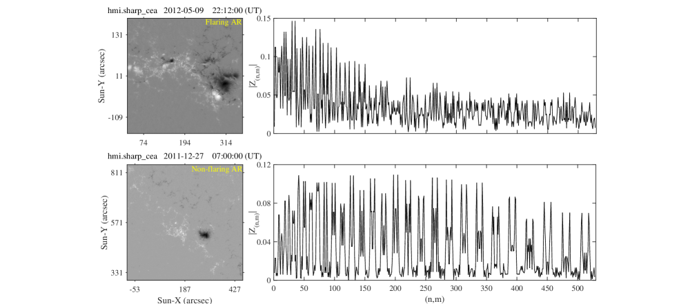
Figure 1: Absolute value of the Zernike moments versus indices $(n,m)$ for a typical AR in the positive class (top panel), and a typical AR in the negative class (bottom panel). Note that each point on the horizontal axis is designated by a pair of integers $(n,m)$ delimited by the third property of the Zernike polynomials which is $|n\pm m|=\rm{even}$. In the case of $N=31$ it means that $n$ takes values from 1 through 31. Applying the third confinement rule of the Zernike Polynomials yields 528 pairs of $(n,m)$ in the following way: when $n=0$ the only possible number for $m$ is 0, if $n=1$ the acceptable numbers for $m$ are $+1$, $0$, and $-1$, and so on.

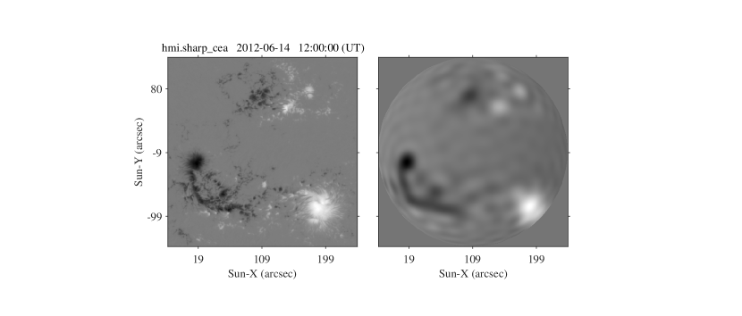
Figure 2: Reconstructed image using the first 528 ($N=31$) Zernike moment terms for a magnetogram image of NOAA active region number 11504 on 14 June 2012 at 12:00 UT which is in the positive class. Left: Radial component ($B_{r}$) magnetogram. Right: Reconstruction of the left-hand side image using the first 528 ZM terms.

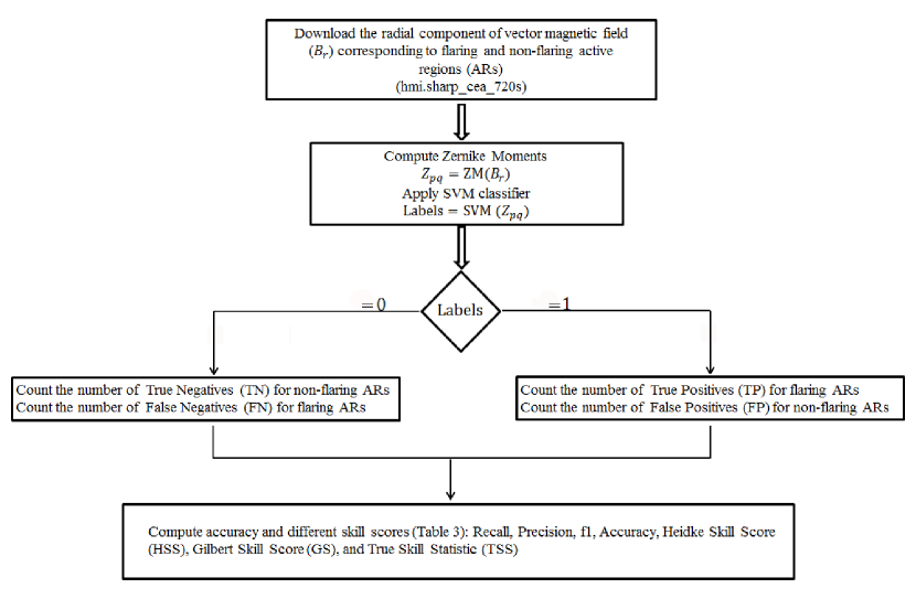
Figure 3: The flowchart of our proposed method.

3 Results

In this paper, using the unique and invariant properties of ZMs of the photospheric magnetogram images and the SVM classifier, we attempt to predict which of the ARs at hand will produce at least one large flare within 48 hours. We divide the whole data set into a training and a test set. A supplement to this paper provides electronic tables which contain the ZMs calculated for each magnetogram in the training and test data sets as MATLAB structures, with the exact time and the NOAA AR numbers given for each one. The ARs used in this paper consist in total of 422 different NOAA active regions observed during the time period 2 June 2010 to 1 August 2016. The training set consists of a total of 85 different NOAA ARs belonging to the positive class observed in the time period 2 June 2010 to 1 June 2014, meaning they produced at least one large flare within 48 hours, and 208 different NOAA ARs belonging to the negative class observed in the same period, meaning they did not produce a large flare within the same time interval. Empirically, in the process of training the positive class to the SVM we use 6, 2, 2, 2, 2, 2, 2, and 2 magnetogram images (20 in total) from 1, 5, 18, 20, 22, 24, 25, and 48 hours, respectively before the flaring time of each of the 85 ARs (Table 1). Also, the data used to train the negative class to the SVM consists of almost 7 magnetogram images for each of the 208 ARs that did not produce any large flare within the past 48 hours. The SVM was trained on the ZMs extracted from this data set.

Table 1: Number of positive class magnetograms corresponding to each time interval before the flaring time used in the training set.

Hours before each large flare	Number of magnetograms
1	6
5	2
18	2
20	2
22	2
24	2
25	2
48	2

The rest of the data are taken as the test set, which consists of 129 ARs. We pretend that we don’t know whether these ARs are positive or negative. There are at most 4 magnetogram images in four different times for each the ARs inside the test set. The goal is to identify the corresponding class for every magnetogram image in the test set.

Analysis of the output of the classifier is presented in Table 2, in which TP (True Positive) denotes the number of flaring ARs that are correctly classified as being a member of the positive class (375), FP (False Positive) denotes the total number of non-flaring ARs that are incorrectly classified as being a member of the positive class (21), TN (True Negative) denotes the total number of non-flaring ARs that are correctly classified as being a member of the negative class (158), and FN (False Negative) denotes the total number of flaring ARs that are incorrectly classified as being a member of the negative class (10).

Table 2: The results of flare prediction using the Zernike moments and the SVM classifier.

True Positive (TP)	False Negative (FN)	True Negative (TN)	False Positive (FP)
375	10	158	21

It is common to assign scores to assess the accuracy of prediction (Wheatland, 2005; Barnes & Leka, 2008). Several skill scores have been proposed and applied for solar flare predictions. Table LABEL:tab3 represents different skill scores and their related formulae. These metrics are gathered from different papers on the subject of flare forecasting (Woodcock, 1976; Barnes & Leka, 2008; Mason & Hoeksema, 2010; Bloomfield et al., 2012; Bobra & Couvidat, 2015; Bloomfield et al., 2016).

Table 3: Performance metrics of the SVM classifier in predicting large flares compared with other authors. We use the first 528 Zernike moments of the magnetogram images. The results of other forecasting methods – Bobra #1 and Bobra #2 (Bobra & Couvidat, 2015); Mason (Mason & Hoeksema, 2010); Ahmed (Ahmed et al., 2013); Barnes (Barnes & Leka, 2008); Bloomfield (Bloomfield et al., 2012); Yu (Yu et. al., 2009); Song (Song et. al., 2009) – that are described in this table are duplicated from Bobra & Couvidat (2015). Bobra #1 and Bobra #2 represent the results that are given in the first column of Table 2 and Table 3 of Bobra & Couvidat (2015), respectively.

Metric	This paper	Bobra #1	Bobra #2	Mason	Ahmed	Barnes	Bloomfield	Yu	Song
	48h	48h	48h	6h	48h	24h	24h	48h	24h
Recall+	0.974	0.714 $\pm$ 0.048	0.869 $\pm$ 0.036	0.617	0.677	NA	0.704	0.817	0.647
Recall-	0.882	0.989 $\pm$ 0.003	0.947 $\pm$ 0.007	0.695	0.994	NA	NA	NA	0.974
Precision+	0.946	0.797 $\pm$ 0.050	0.501 $\pm$ 0.041	0.008	0.877	NA	0.146	0.831	0.917
Precision-	0.940	0.983 $\pm$ 0.003	0.992 $\pm$ 0.002	0.998	0.980	NA	NA	NA	0.860
$f_{1}^{+}$	0.959	0.751 $\pm$ 0.032	0.634 $\pm$ 0.033	0.015	0.764	NA	0.242	NA	0.758
$f_{1}^{-}$	0.910	0.986 $\pm$ 0.002	0.969 $\pm$ 0.003	0.819	0.987	NA	NA	NA	0.913
Accuracy	0.945	0.973 $\pm$ 0.003	0.943 $\pm$ 0.006	0.694	0.975	0.922	0.830	0.825	0.873
$\rm{HSS}_{1}$	0.919	0.528 $\pm$ 0.062	-0.008 $\pm$ 0.142	-78.9	0.581	0.153	NA	NA	0.588
$\rm{HSS}_{2}$	0.871	0.737 $\pm$ 0.034	0.606 $\pm$ 0.035	0.008	0.751	NA	0.190	0.650	0.676
GS	0.771	0.585 $\pm$ 0.043	0.436 $\pm$ 0.036	0.004	0.601	NA	NA	NA	0.510
TSS	0.856	0.703 $\pm$ 0.047	0.817 $\pm$ 0.034	0.312	0.671	NA	0.539	0.650	0.620

Table 3 lists the prediction metrics achieved by the present algorithm compared to the scores of other works. Bobra & Couvidat (2015) provided two tables (Tables 2 and 3 therein) to compare the values of skill scores obtained by different forecasting methods. Other than the second column of Table 3, all other columns are a copy of Tables 2 and 3 of Bobra & Couvidat (2015).

Barnes & Leka (2008) concluded that even if different databases are used for prediction, comparison of the skill scores for different methods is meaningful. However, unless the datasets are identical, there is no completely meaningful comparison between two or more different methods that one could make. Hence, one should not consider the results of Table 3 as an absolute reference for comparison between the methods.

The second column of Table 3 lists the skill scores of the present algorithm for the classification process (see the two supplementary electronic tables). The third and fourth column of Table 3 list the performance metrics achieved by Bobra & Couvidat (2015), for specifically tuned SVMs which result in the highest HSS₂, and TSS scores respectively. Their method was demonstrated to predict large solar flares within 48 hours before occurrence with a TSS score of $0.817$. The second-highest TSS in the table belongs to Ahmed et al. (2013) which is $0.671$. As Table 3 shows, the TSS score achieved in the present work is 0.856. Also, the highest HSS₂ score amongst all other previous methods, given by Ahmed et al. (2013), is $0.751$ and the second-highest HSS₂ score belongs to Bobra & Couvidat (2015), which is $0.737$. The HSS₂ score attained with the present method is 0.871. Another metric of interest here is the Recall⁺. As it is shown in Table LABEL:tab3, the Recall⁺ score is associated with the number of FNs and TPs, which characterize the ability of the classifier to achieve the least number of FNs. The reason for this interest is that if a positive event is falsely reported as being a negative one, the resulting costs for this lack of accuracy in prediction could be devastating. Mis-prediction of negative events (i.e. false positive, FP) may only require, for example, powering off a power plant, or rotating a satellite’s shields towards the Sun, but when it is reported to an astronaut in deep space that they are unlikely to be hit by a large flare within some time, the consequence of error is more serious. The highest Recall⁺ score among former methods is $0.869$ due to Bobra & Couvidat (2015), and the second-highest Recall⁺ is $0.817$, due to Yu et. al. (2009). The Recall⁺ score gained by the present method is 0.974.

4 Discussion

Here, we propose a method based on the properties of ZMs (Zernike Moments) of magnetogram images for ARs (Active Regions), and the Support Vector Machine for prediction of large (M and X type) solar flares.

Previous methods have used a few parameters extracted from AR magnetograms (e.g. the total unsigned current helicity, the total magnitude of the Lorentz force, the total photospheric magnetic free energy density, and the total unsigned vertical current) as the basis for classification (e.g. Leka & Barnes, 2003; Bobra & Couvidat, 2015; Barnes et al., 2016). One may ask, is it possible that two different magnetic fields yield the same values for above mentioned parameters? Suppose we have two arbitrary three dimensional vector magnetic field magnetograms observed at the solar photosphere ($z=0$), ${\bf B}_{1}(x,y)$ and

$${\bf B}_{2}(x,y)={\bf B}_{1}(x,y)+\nabla\phi(x,y).$$ (6)

These two magnetic fields lead to the same total current helicity

$$\sum B_{2z}J_{2z} = \sum\frac{1}{\mu_{0}}(\nabla\times{\bf B}_{2})_{z}B_{2z}$$ (7)

$$= \sum\frac{1}{\mu_{0}}(\nabla\times{\bf B}_{1})_{z}B_{1z}$$

$$= \sum B_{1z}J_{1z},$$

and the same total flux

$$\sum B_{1z}(x,y)dxdy=\sum B_{2z}(x,y)dxdy.$$ (8)

Since the total free energy density and the total Lorentz force are both proportional to $B^{2}$, applying an additional constraint,

$$2\frac{\partial\phi}{\partial x}B_{1x}+\left(\frac{\partial\phi}{\partial x}\right)^{2}=-2\frac{\partial\phi}{\partial y}B_{1y}-\left(\frac{\partial\phi}{\partial y}\right)^{2},$$ (9)

results in

$$B_{1}^{2}=B_{2}^{2},$$ (10)

and hence the total free energy density and the total Lorentz force for the two magnetic fields are the same. Assume that these two vector magnetic field represent the photospheric magnetic field for two arbitrary ARs. It may happen that one of the magnetic fields corresponds to a flare productive AR and the other corresponds to a non-flaring AR. In this case a classification process based on helicity, total flux, total free energy, and total Lorentz force will not discriminate between the two ARs, since these two different magnetic fields have the same values for above mentioned parameters. In other words, there could be two different vector magnetic fields for two ARs having an identical vector in the feature space. This can obviously affect the results of the classification. It can be seen that the ZMs for these two magnetic fields given by Equation (3) represent two different sets of values.

Moreover, as discussed in Barnes et al. (2016), performance comparisons between different flare forecasting methods based on extracting a few parameters out of AR magnetograms indicate that there is no clearly superior method, and it was pointed out that this might be due to correlations between the parameters. Also, the methods were found to have a rather weak performance in achieving high positive skill scores. An advantage of the present method is that the Zernike moments provide unique information as a basis for classification of an AR by comparison with a few global parameters (e.g., total flux, current helicity etc). Further, the present method is demonstrated to be able to predict solar flares with a small number of FNs rather than just reducing the number of FPs. This has important practical consequences for reducing the costs of errors in prediction (e.g. Bobra & Couvidat 2015).

We thank NASA/SDO, the HMI Science Team, and NOAA for the availability of the SDO/HMI data and the GOES flare catalogue used here.

Appendix

4.1 The Support Vector Machine

The purpose of the SVM classifier is to find a decision boundary with a margin as large as possible, to reduce the classification error. Suppose that $D$ is a binary-class training set with $N$ data points in the $l$-dimensional feature $(x_{1},...,x_{l})$ space, that is

$$D=\bigg{\{}(x_{i},y_{i})|x_{i}\in R^{l},y_{i}\in\{-1,+1\})\bigg{\}},~{}~{}i=1,{\cdots},N.$$ (11)

Constructing a decision boundary, which is a separating hyperplane in a high-dimensional space, SVM can segregate classes. This hyperplane is given by

$$\textbf{w}\cdot\boldsymbol{\Phi}(\textbf{x})+b=0,$$ (12)

where

$$\boldsymbol{\Phi}:R^{l}\rightarrow R^{L},~{}~{}~{}~{}~{}~{}~{}~{}L\geq l,$$ (13)

and where w and $b$ are a weight vector and bias, respectively. $\boldsymbol{\Phi}(\textbf{x})$ is a linear or nonlinear vector function that maps each data point $\textbf{x}_{i}$ into the feature space in high-dimensional space. These parameters, namely w and $b$, can be computed by solving the following optimization problem:

$$\min_{\textbf{w},b,\xi}~{}~{}\dfrac{1}{2}||\textbf{w}^{2}||+c\sum_{i=1}^{N}{\xi_{i}},$$ (14)

subject to (the constraint):

$$y_{i}(\textbf{w}\cdot\textbf{x}_{i}+b)\geq 1-\xi_{i},~{}~{}~{}~{}~{}~{}~{}~{}\xi_{i}\geq 0,$$ (15)

where $\xi_{i}$ and $c$ are the error value for the decision boundary and the regularization parameter, respectively. The regularization parameter controls the trade-off between the margin width and model complexity and is determined by the user. The equations given above can be converted into the following dual form:

$$\max_{\alpha}~{}~{}\sum_{i=1}^{N}\alpha_{i}-\dfrac{1}{2}\sum_{i=1}^{N}\sum_{j=1}^{N}y_{i}y_{j}\alpha_{i}\alpha_{j}K(x_{i},x_{j}),$$ (16)

subject to

$$\sum_{i=1}^{N}y_{i}\alpha_{i}=0,~{}~{}~{}~{}~{}~{}~{}~{}\alpha_{i}\geq 0,~{}~{}~{}~{}~{}~{}~{}~{}\forall i:0\leq i\leq c,$$ (17)

where $\alpha_{i}$ is the Lagrange multiplier corresponding to the $i^{\rm th}$ training sample and $K(x_{i},x_{j})$ is a Kernel function which maps the input vectors into a suitable feature space to achieve a better representation. So, we have $K(x_{i},x_{j})=\boldsymbol{\Phi}(\textbf{x}_{i})\cdot\boldsymbol{\Phi}(\textbf{x}_{j})$. This is a constrained optimization problem and it can be solved by a Lagranian multiplier method. The output of SVM for each input data point is equal to

$$y(x)=\rm{sgn}[\textit{f}(\textit{x})],$$ (18)

where

$$f(x)=\sum_{i=1}^{N}y_{i}\alpha_{i}K(x_{i},x_{j})+b.$$ (19)

Usually after training the SVM, the value of Lagrange multiplier is zero for many training points. Support vectors are input vectors that just touch the boundary of the margin (see e.g. Qu et al., 2003; Theodoridis & Koutroumbas, 2009; Hsu et al., 2011).

References

- Abramenko (2015) Abramenko, V. I. 2015, Geomagnetism & Aeronomy, 55, 860
- Ahmed et al. (2013) Ahmed, O. W., Qahwaji, R., Colak, T., Higgins, P. A., Gallagher, P. T., & Bloomfield, D. S. 2013, SoPh, 283, 157
- Alipour et al. (2012) Alipour, N., Safari, H., & Innes, D. E. 2012, ApJ, 746, 8
- Alipour & Safari (2015) Alipour, N. & Safari, H. 2015, ApJ, 807, 9
- Barnes & Leka (2008) Barnes, G. & Leka, K. D. 2008, ApJ, 688L, 107
- Barnes et al. (2016) Barnes, G., Leka, K.D., Schrijver, C.J., Colak, T., Qahwaji, R., Ashamari, O.W., Yuan, Y., Zhang, J., McAteer, R.T.J., Bloomfield, D.S., Higgins, P.A., Gallagher, P.T., Falconer, D.A., Georgoulis , M.K., Wheatland, M.S., Balch, C., Dunn, T., and Wagner, E.L. 2016, ApJ, 829, 89
- Bélanger et al. (2007) Bélanger, E., Vincent, A., & Charbonneau, P. 2007, SoPh, 245, 141
- Bloomfield et al. (2012) Bloomfield, D. S., Higgins, P. A., McAteer, R. T. J. & Gallagher, P. T. 2012, ApJ, 747, L41
- Bloomfield et al. (2016) Bloomfield, D.S., Gallagher, P.T., Marquette, W.H., Milligan, R.O., & Canfield, R.C. 2016, SoPh, 291, 411
- Bobra & Couvidat (2015) Bobra, M. G. & Couvidat, S. 2015, ApJ, 798, 11
- Bobra & Ilonidis (2016) Bobra, M. G., & Ilonidis, S. 2016, ApJ, 821, 127
- Boucheron et al. (2015) Boucheron, L., Al-Ghraibah, A., & McAteer, J. 2015, ApJ, 812, 11
- Colak & Qahwaji (2009) Colak, T., & Qahwaji, R. 2009, Space Weather, 7, S06001
- Crown (2012) Crown, M. D. 2012, Space Weather, 10, S06006
- Falconer et al. (2008) Falconer, D. A., Moore, R. L., & Gary, G. A. 2008, ApJ, 689, 1433
- Falconer et al. (2011) Falconer, D. A., Barghouty, A. F., Khazanov, I., & Moore, R. 2011, Space Weather, 9, S04003
- Georgoulis & Rust (2007) Georgoulis, M. K. & Rust, D. M. 2007, ApJ, 661, L109
- Georgoulis et al. (2012) Georgoulis, M. K. & Rust, D. M., Tziotziou, K., and Raouafi, N. 2012, ApJ, 759, 18
- Guerra & Pulkkinen (2015) Guerra, J. A., Pulkkinen, A., & Uritsky, V. M. 2015, Space Weather, 13, 626
- Gunn (1997) Gunn, S. R. 1997, Technical Report, Image Speech and Intelligent Systems Research Group, Univ. Southampton
- Hoeksema et al. (2014) Hoeksema, J. T., Liu, Y., Hayashi, K., Sun, X., Schou, J., Couvidat, S., Norton, A., Bobra, M., Centeno, R., Leka, K. D., Barnes, G., & Turmon, M. 2014, SoPh, 289, 3483
- Hosny (2010) Hosny, K. M. 2010, Information Sciences, 180, 2299
- Hsu et al. (2011) Hsu, C. C., Wang, K. S., Chang, S. H. 2011, Expert Systems with Applications 38, 4698
- Huang et al. (2013) Huang, X., Zhang, L., Wang, H., & Li, L. 2013, Astron. Astrophys., 549, 6
- Javaherian et al. (2014) Javaherian, M., Safari, H., Amiri, A. & Ziaei, S. 2014, SoPh, 289, 3969
- Khotanzad (1990) Khotanzad, A. 1990, IEEE Trans. Pattern Anal. Mach. Intell., 12, 489
- Künzel (1960) Künzel, H. 1960, Astron. Nachr., 285, 271
- Leka & Barnes (2003) Leka, K. D. & Barnes, G. 2003, ApJ, 595, 1277
- Leka & Barnes (2007) Leka, K. D. & Barnes, G. 2007, ApJ, 656, 1173
- Liao & Pawlak (1998) Liao, S., X. & Pawlak, M. 1998, IEEE Transactions on Pattern Analysis and Machine Intelligence, 20, 12, 1358
- Mason & Hoeksema (2010) Mason, J. P., & Hoeksema, J. T. 2010, ApJ, 723, 634
- McIntosh (1986) McIntosh, P. S. 1986, Bull. Am. Astron. Soc., 18, 851
- McIntosh (1990) McIntosh, P. S. 1990, SoPh, 125, 251
- Priest & Forbes (2002) Priest, E. R. & Forbes, T. G. 2002, Astron. Astrophys. Rev., 10, 313
- Pulkkinen (2007) Pulkkinen, T. 2007, Living Rev. Solar Phys., 4, 1
- Qu et al. (2003) Qu, M., Shih, F., Jing, J., Wang, H. 2003, SoPh, 217, 157
- Rust (1993) Rust, D. 1993, Eos, Trans. Amer. Geophys. Union, 74, 553
- Sammis et al. (2000) Sammis, I., Tang F., & Zirin, H. 2000, ApJ, 540, 583
- Schou et al. (2012) Schou, J., Scherrer, P. H., Bush, R. I. et al. 2012, SoPh, 275, 229
- Schrijver et al. (2007) Schrijver, C. J. 2007, ApJ, 655, L117
- Schwenn (2006) Schwenn, R. 2006, Living Rev. Solar Phys., 3, 2
- Shin et al. (2016) Shin, S., Lee, J., Moon, Y., Chu, H., & Park, J. 2016, SoPh, 291, 897
- Song et. al. (2009) Song, H., Tan, C., Jing, J., Wang, H., Yurchyshyn, V., & Abramenko, V. 2009, SoPh, 254, 101
- Strugarek & Charbonneau (2014) Strugarek, A. & Charbonneau, P. 2014, SoPh, 289, 4137
- Tan, Steinbach & Kumar (2006) Tan, P. N., Steinbach, M., & Kumar, V., Introduction to Data Mining, Addison-Wesley, International Edition 2006, 256
- Theodoridis & Koutroumbas (2009) Theodoridis, S., Koutroumbas, K. 2009, Pattern Recognition, 4rd edn., Academic Press, Elsevier Inc
- Vapnik (1995) Vapnik, V. N. 1995, The nature of statistical learning theory. Berlin Heidelberg, Springer-Verlag
- Wheatland (2004) Wheatland, M. S. 2004, ApJ, 609, 1134
- Wheatland (2005) Wheatland, M. S. 2005, Space Weather, 3
- Woodcock (1976) Woodcock, F. 1976, Monthly Weather Review, 104, 1209
- Yang et al. (2013) Yang, X., Lin, G., Zhang, H., & Mao, X. 2013, ApJ, 744, L27
- Yu et. al. (2009) Yu, D., Huang, X., Wang, H., & Cui, Y. 2009, SoPh, 255, 91
-
Yuan et al. (2010)
Yuan, Y., Shih, F., Jing, J., & Wang, H. 2010 ,
Research in Astron. Astrophys., 10, 785 - Zernike (1934) Zernike, F. 1934, Physica, 1, 689